An Optimal Wheel Torque Control on a Compliant Modular

Robot for Wheel-Slip Minimization

Siravuru Avinash1, Suril V Shah1, and K Madhava Krishna1

1 Robotics Research Centre, ,

International Institute of Information Technology, Hyderabad, 500032, India. ,

avinash.siravuru@research.iiit.ac.in, surilshah@iiit.ac.in, mkrishna@iiit.ac.in

Abstract

This paper discusses the development of an optimal wheel torque controller for a

compliant modular robot. The wheel actuators are the only actively controllable ele-

ments in this robot. For this type of robots, wheel-slip could offer a lot of hindrance

while traversing on uneven terrains. Therefore, an effective wheel-torque controller

is desired that will also improve the wheel-odometry and minimize power consump-

tion. In this work, an optimal wheel-torque controller is proposed that minimizes the

traction-to-normal force ratios of all the wheels at every instant of its motion. This

ensures that, at every wheel, the least traction force per unit normal force is applied

to maintain static stability and desired wheel speed. The lower this is, in compari-

son to the actual friction coefficient of the wheel-ground interface, the more margin

of slip-free motion the robot can have. This formalism best exploits the redundancy

offered by a modularly designed robot. This is the key novelty of this work. Exten-

sive numerical and experimental studies were carried out to validate this controller.

1

The robot was tested on four different surfaces and we report an overall average slip

reduction of 44 % and mean wheel-torque reduction by 16 %.

Nomenclature

φi Relative angle between links i and i+ 1

τwi Torque applied at wheel i

θi Absolute angle of link i

c Clearance between wheel center and trunk

Fi Traction force at Wheel i

fxli X component of the trunk-joint reaction force between trunks i and i+ 1

fxwi X component of the wheel-joint reaction force on the trunk due to wheel i

fyli Y component of the trunk-joint reaction force between trunks i and i+ 1

fywi Y component of the wheel-joint reaction force on the trunk due to wheel i

ki Spring constant of spring i

l Length of the trunk

l0 Offset distance between trunk-joint and wheel joint

ml Mass of the trunk

mw Mass of the wheel

Ni Normal force at Wheel i

r Radius of the wheel

Si Spring i

Wi Wheel i

wl Weight of the trunk (mlg)

2

ww Weight of the wheel-pair (2mwg)

1 Introduction

Wheeled robots with enhanced traversing ability will play a crucial role in search and

rescue operations, planetary exploration, etc. It is highly desired that the robot sustains

forward motion without losing stability throughout its operation. The extent to which a

robot can achieve this on a general unstructured terrain defines its Terrainability [1]. In

a search and rescue operation, the terrain knowledge is generally unknown before hand.

Therefore, it is important and useful to have high terrainability. We have proposed a novel

compliant modular robot that can ascend obstacles upto three times its wheel diameter.

The robot’s design details and its climbing ability were shown in [2]. We later expanded

this compliant joint design to enable the robot to successfully descend from equally big-

sized obstacles. However, it was observed that the conventional velocity controllers used

for generating forward motion resulted in considerable amount of wheel-slip while climbing

steep obstacles (like steps). Wheel-slip typically hinders continuous forward motion and

severely effects the accuracy of wheel odometry. Therefore, this work attempts to improve

the terrainability of the robot by minimizing wheel slip. A viable solution to this problem

is to proactively maintain the least possible traction-to-normal force ratios at all the wheels

throughout the traversal. This objective was formulated as an wheel torque optimization

problem and the underlying theory was presented in [3]. Multiple objective functions

that capture the notion of wheel-torque minimization were considered and their respective

merits and demerits were presented. In the present work, we build a controller based on

the wheel torque optimizer developed in [3] and apply it to the numerical and experimental

3

(a) (b)

Figure 1: Snapshots of the a) Compliant Modular Robot and b) the Sectional View of a2-module CAD Model

models of the robot to validate its efficacy.

Wheel-Slip minimization is well studied for SHRIMP [4, 5] and CRAB [6, 7, 8, 9]

robots. However, it may be noted that the direct application of the formalism shown in

these works to a compliant modular robot is non trivial. In the case of the above-mentioned

single module robots, the wheels always maintain contact with the ground during rough

terrain traversal. Therefore, a generalized set of static stability equations can be derived

to analyze the robots motion. However, in the case of multi-module compliant robot,

wheel-ground contact is not always guaranteed or desirable [2]. Accordingly, appropriate

changes take place in the static stability equations. This is systematically analyzed in

this paper. Additionally, extensive numerical and experimental studies were conducted,

and a consistent and significant reduction in slip rate was noted after the application of

the new optimal wheel-torque based controller. In contrast to the results shown in the

previous work [8], the slip rate reduction is consistently significant along a wide range of

coefficients of friction. This further validates the advantages of a modular and compliant

design. This forms the main contribution of this work. Also, a notable reduction in mean

4

torque requirement was noted at all the wheels, thereby improving the energy efficiency

of the robot. Figure 1 shows the prototype of the proposed robot mechanism, along with

its sectional view.

The remaining paper is organized as follows. In Section 2, the compliant modular robot

mechanism is introduced, and its quasi-static analysis is provided. Section 3 introduces

wheel-slip and presents a systematic procedure to perform wheel torque optimization to

minimize slippage. Section 4 analyzes the optimization results in order to choose the best

objective function. In Section 5, a controller is developed to achieve the desired optimal

wheel torque. Numerical and Experimental results validating the effectiveness of this

controller are also provided. Finally, Section 6 contains the conclusions and outline for

future work.

2 Model Description

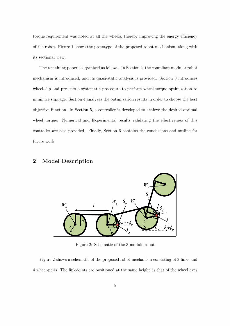
Figure 2: Schematic of the 3-module robot

Figure 2 shows a schematic of the proposed robot mechanism consisting of 3 links and

4 wheel-pairs. The link-joints are positioned at the same height as that of the wheel axes

5

with an offset(l0) equal to the wheel’s radius. The joints at wheels and links are denoted

by W1 −W4 and J1 − J2, respectively. The location of the passive springs is denoted by

S1 and S2, respectively. Finally, φi is the relative joint angle between links i and i+ 1 and

θi be the absolute joint angle of link i with respect to the ground.

The springs at S1 and S2 have stiffnesses 0.04 Nm/rad and 0, respectively. (Joint J2

is fully passive). A more comprehensive discussion on the robot’s compliance design is

given in [2]. A 900 double torsion spring is designed for this purpose. It is close wound

and having tangent legs. It is fitted into the joint J1 with zero preload. The robot’s

specifications are provided in Table 1.

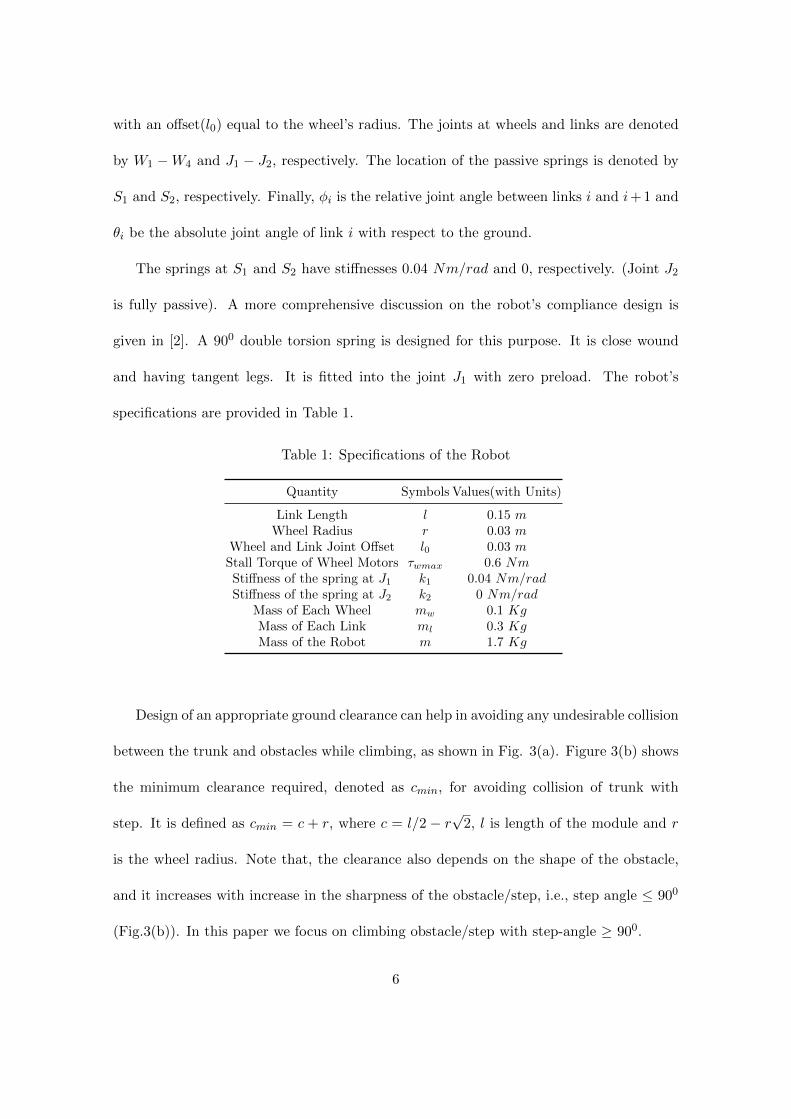
Table 1: Specifications of the Robot

Quantity Symbols Values(with Units)

Link Length l 0.15 mWheel Radius r 0.03 m

Wheel and Link Joint Offset l0 0.03 mStall Torque of Wheel Motors τwmax 0.6 NmStiffness of the spring at J1 k1 0.04 Nm/radStiffness of the spring at J2 k2 0 Nm/rad

Mass of Each Wheel mw 0.1 KgMass of Each Link ml 0.3 KgMass of the Robot m 1.7 Kg

Design of an appropriate ground clearance can help in avoiding any undesirable collision

between the trunk and obstacles while climbing, as shown in Fig. 3(a). Figure 3(b) shows

the minimum clearance required, denoted as cmin, for avoiding collision of trunk with

step. It is defined as cmin = c + r, where c = l/2 − r√

2, l is length of the module and r

is the wheel radius. Note that, the clearance also depends on the shape of the obstacle,

and it increases with increase in the sharpness of the obstacle/step, i.e., step angle ≤ 900

(Fig.3(b)). In this paper we focus on climbing obstacle/step with step-angle ≥ 900.

6

Figure 3: Effect of ground clearance: a) An inevitable collision occurs when the moduleis designed with insufficient ground clearance; b) The minimum ground clearance cmin isparametrized in terms of the length of the module(l) and the wheel radius(r).

2.1 Climbing Analysis with a Passive Modular Robot

Fig. 4(a) shows the climbing phase of the robot with fully passive joint J1 (no spring).

Note that module 1 will continue to climb along the step till it crosses a limiting angle.

Beyond the limiting angle the module will tip-over as shown in Fig. 4(b). The limiting

angle called tip-over angle (θto) (Fig. 4(a)) can be determined based on the position of

center-of-mass (COM) of the module as θto = π/2 − tan−1(yCOM/xCOM ), where xCOM

and yCOM denote the COM coordinates of the module in the module fixed frame. This

tip-over phenomenon limits the climbing ability of the proposed robot, and the robot can

only climb obstacles of heights less than or equal to lsin(θto). In our previous work [2],

was shown how adding an optimally designed torsional spring at joint J1 helped avoided

θ1 crossing θto by lifting module 2 off the ground. This causes φ1 to decrease while keeping

θ1 nearly constant. This enables the robot to climb higher without having to tip-over.

The aim of this paper is to only use the traction forces developed at the wheel-ground

contacts to climb steps. The passive link joints allow the mechanism to freely deform

7

Figure 4: Climbing behavior of the passive robot: a) In the climbing phase, it continuesto climb the step as long as φ1 ≤ θto. b) If the module continues to climb beyond thispoint, then the moment due to its self-weight changes direction and causes the module totip over. This phase is called tip over phase.

along an obstacle. For the experiments in this work, the proposed compliant modular

robot traverses at a constant speed of 18cm/s. At such low speeds the dynamic effects are

minimal and quasi-static analysis gives a good overview of the forces acting on the robot.

Wheel torques typically are responsible for balancing these external forces and maintain

static equilibrium. As the robot is symmetric about the sagittal plane, a planar analysis

provides a good approximation of its performance while climbing steep obstacles (assuming

that they are also symmetric about the sagittal plane). Static stability equations of the

robot are derived in the next subsection.

2.2 Quasi-Static Model of the Modular Robot

A generic set of static equilibrium equations cannot be employed for analyzing and op-

timizing the modular robot’s step climbing maneuver as it was shown in [10]. In the

PAW([10]) robot and other passive suspension robots like SHRIMP([11]) and CRAB([8]),

wheels always maintained contact with the ground. But in the case of the proposed robot,

8

wheel-pairs may lift off the ground, where necessary, to avoid tipping over. This slightly

complicates the quasi static analysis as the static equilibrium equations change when there

is a phase change, during the climbing maneuver. Therefore, the robot’s static model is

divided into two phases, as shown in Fig. 5.

(a) Phase-1: one link climbing at any instant

(b) Phase-2: two links climbing at any instant

Figure 5: Snapshots showing the various forces and moments acting on therobot during the 2 climbing phases

This division is essential as the forces and moments acting on the robot change from

one phase to the other. Every time a wheel-pair lifts off the ground, its corresponding

normal and traction forces are lost and an additional counter moment is generated due

to the spring at the corresponding link joint. This changes the∑Fy (net force acting

9

in the y -direction),∑Fx (net force acting in the x-direction) and

∑M ’s (net moments

about J1 and J2), which have to be appropriately adjusted to maintain static equilibrium.

Therefore, when every subsequent wheel is lifted off the ground, the robot transits from

one climbing phase to the other. Equations (1-5) and (6-10) contain the minimal set of

static-equilibrium equations for the first and second phases of climbing of the robot as

shown in Figs. 5(a)-(b), respectively.

∑Fx = 0 N1 − F2 − F3 − F4 = 0 (1)∑Fy = 0 3wl + 4ww − F1 −N2 −N3 −N4 = 0 (2)∑MJ1 = 0 F1(lcosφ1 + r) +N1lsinφ1 − wl[(l/2)cosφ1-csinφ1]

− k1φ1 − wwlcosφ1 = 0 (3)∑MJ2 = 0 F2r +N2l − wwl − wl(l/2)− [wl + ww − F1](l + l0)− k2φ2 + k1φ1 = 0 (4)∑MW4 = 0 F3r +N3l − wwl − wl(l/2)− [2(wl + ww)− F1 −N2](l + l0) + k2φ2 + F4r = 0

(5)

∑Fx = 0 N1 − F3 − F4 = 0 (6)∑Fy = 0 3wl + 4ww − F1 −N3 −N4 = 0 (7)∑MJ1 = 0 F1(lcos(φ1 + φ2) + r) +N1lsin(φ1 + φ2)− wl[(l/2)cos(φ1 + φ2)− csin(φ1 + φ2)]

− k1φ1 − wwlcos(φ1 + φ2) = 0 (8)∑MJ2 = 0 [F1 − (wl + ww)](l + l0)cosφ2 − wl(l/2cosφ2 − csinφ2)

− wwlcosφ2 + k1φ1 − k2φ2 +N1(l + l0)sinφ2 = 0 (9)∑MW4 = 0 F3r +N3l − wwl − wl(l/2)− [2wl + 2ww − F1](l + l0) + k2φ2 + F4r = 0 (10)

These equations are obtained from by simplifications and substitutions of the force-moment

10

equations given in Appendix A. In the first phase, only link 1 is climbing while the other links (and

wheels) are on the ground supplying the required push force. Similarly, in the second phase, links

1 and 2 are involved in climbing at any instant. It is expected that the robot can climb heights

upto lsinθto with 1 climbing link and between lsinθto and 2lsinθto using 2 links. In this paper,

the analysis is limited to heights requiring at most 2 climbing links, thus ensuring that there are

always 2 wheel-pairs on the ground to provide sufficient traction at any given point.

It can be seen that there are five equations per phase. The first two equations ensure the

equilibrium of forces in the x and y directions, respectively. The remaining equations denote the

moment equilibrium at the 2 link joints J1 and J2, and a wheel joint W4, respectively. Note that,

ww = 2mwg and wl = mlg where mw and ml denote the masses of the wheel and link, respectively.

Fi and Ni are the traction and normal forces acting on the ith wheel, respectively. ki is the spring

constant of the spring acting at the ith link joint to maintain static equilibrium at an arbitrary

configuration.

The optimal spring stiffness values were obtained for climbing big step-like obstacles while

avoiding tip-over in [2]. Only one spring is required at joint J1 to climb a height of upto 17cm. Its

spring constant is given in Table 1. With the addition of springs at the link joints, this modular

robot can successfully climb the rise of a step upto twice its link length with the help of only

wheel traction. However, wheel torques can be used to control this step climbing only under the

assumption that there will be no slippage. So this passive compliant robot design cannot be fully

exploited without ensuring that the wheel-slip is minimized. In the next section, the causes of

wheel-slip are discussed and an optimization formulation with an objective to avoid slippage is

described. It was shown in [2] that for a given height h, an n-modular compliant robot with m

compliant joints could be developed. As an extension, it can be ascertained that such a robot will

have m + 1 climbing phases. With out loss of generality, this method can be easily extended to

determine optimal wheel torques of the robot’s n+1 wheel-pairs. In the next section, the wheel-slip

problem is introduced and potential solutions are suggested.

11

3 Wheel-Slip Reduction

Figure 6: Free body diagram of the wheel

Figure 6 shows the free-body diagram of a wheel rolling on a flat surface. It can be noted that,

the wheel is in static equilibrium when F = τ/r, where r and τ are the wheel‘s radius and torque,

respectively. For the wheel to maintain pure rolling, the frictional force F should always satisfy

the friction constraint equations, F = µsN , where µs is the coefficient of static friction. Here, F

is directly proportional to the wheel torque τ . If the wheel torque exceeds µsN , then the wheel

begins to slip and frictional force, F = µdN , where µd is the coefficient of dynamic friction. The

aim is to always keep the wheel torque within the limit of µsN to avoid any slippage. However,

this is very hard to achieve as µ for the wheel-ground interface is not known in advance, and it

also changes dynamically on any terrain. Well known slip reduction technologies like Anti-Lock

Braking System (ABS), which is used extensively in automobiles, are equipped with sensors to

detect wheel-slip and a corrective torque control action is taken till the wheel stops slipping. But

this method requires slip to occur. A preventive method, which is not only robust but also exploits

the robot’s suspension mechanism to minimize slippage is desirable. Note that, slippage doesn’t

hinder the climbing ability of this robot. The robot can still successfully climb even if there is slip

in some of its wheels. However, slip makes it difficult to exercise control on the robot and also

expends energy. Therefore, it is very important to study it carefully and create mechanisms which

can minimize slip.

12

To build this analysis, one may first begin by assuming that there is no slip, and then estimate

the Fi and Ni values across various points on the terrain by minimizing∑i Fi/Ni to achieve the

objective of no slip. Denote the maximum value of the Fi/Ni ratio obtained from this optimization

as µo. The mechanism with lower µo can traverse on a wider range of surfaces (whose µs w.r.t

the wheel is between µo and 1) without slipping. This is the most intuitive objective function for

the optimization procedure, as shown in (11). However, since the function is non-linear, it may

get stuck in local optima. Also note that, this objective function doesn’t enforce all the wheel-

pairs to maintain the same µo value. This can be enforced by using (12) instead. Though these

two objective functions best capture the objective of this optimization procedure, they both are

non-linear and may get stuck in local optima. The objective can be linearized by just minimizing

the sum of traction forces, as shown in (13), instead of minimizing the sum of traction-to-normal

ratios. Since this function is linear it is guaranteed to converge to a global optimum value. The

relative merits of these three objective functions is further analyzed in the subsequent sections and

the best one will be chosen to develop the optimal wheel-torque based controller.

4∑i=1

Fi/Ni (11)

4∑i=1

(Fi/Ni − µavg)2 where, µavg =

4∑i=1

Fi/Ni/4 (12)

4∑i=1

Fi (13)

Before executing the optimization procedure, the constraint equations need to be derived.

Constraint equations capture the static stability requirement of the robot at any intermediate

configuration while step-climbing. To this end, in the next subsection, a method is introduced to

determine the robot’s configuration at any given height.

13

3.1 Posture Estimation

The use of 2-links for climbing at any instant, allows the robot to climb steps/walls as high as

2lsin(θto), i.e., hmax, without tipping over as explained in Section-2.1. To estimate the postures,

the step height is divided into n set points between 0 and hmax, each point separated by the distance

of 0.01m. The posture of the robot at all the set points is determined so that they can to used

to derive the static equilibrium equations for that posture. For step heights that involve only one

climbing link, i.e., heights between 0 and lsin(θto) (phase-1), the posture of the robot, in terms of

the joint angles, can be determined as φj1 = sin−1(hj/l) and φ2 = 0. When φ1 = 700 (phi1 ≈ θto) ,

i.e., after having climbed a height of 0.14m, the robot transits to phase-2. Wheel-pair-2 is lifted off

the ground and the robot now has two climbing members. This process reduces φ1 and increases

φ2 while ensuring that θ1 ≤ θto. The desired postures for the second phase can be obtained by

running a simple optimization procedure for all the heights between lsinθto and 2lsinθto as shown

in (14). The objective function ensures the net change in the relative angles is minimized while

moving from one set-point to the other. This is very important from the quasi-static point of view

as a drastic change in posture with a small increase in height cannot be attained without taking

the dynamics of the system into consideration.

minimizeφ1,φ2

2∑i=1

(φji − φj−1i )2

subject to lsin(φ1 + φ2) + lsin(φ2) = hj

φ1 + φ2 ≤ θto

0 ≤ φ1, φ2 ≤ θto

(14)

This provides the posture desired from the robot at various set-points. The objective functions

have to be minimized across all these set-points to study the robot’s performance and localize

potential regions for slippage.

14

3.2 Optimization Routine

The design variables are Fi’s and Ni’s of all the four wheels. For maintaining an arbitrary posture

of the robot, the static equilibrium equations have to be satisfied at that posture. Thus, they form

the equality constraints to this problem. These equations change from one phase to the other at

the set point lsinθto, to reflect the fact that the second wheel is lifted off the ground. Therefore,

for phase-1, the equality constraints are obtained from (1-5) and for phase-2, it is obtained from

(6-10). As the posture is predetermined for a given height, the equality constraints are linear.

However, since some of the objective functions are non-linear, standard functions like fmincon (of

MATLAB) rely on a strong initial guess provided by the user to search for the globally optimal

value. Providing a good initial guess is hard in this scenario as the optimization routine has to be

run on all the set points and each one may have a good initial guess of its own. An alternative

approach is to further compress the feasible region by tightly bounding the design variables using

the knowledge of their properties and the desired objective. To this end, additional linear inequality

constraints are added to the system to reduce the feasible region and ensure that the proximity of

the obtained solution is as close to the global minimum as possible. Equation (15) is to restrict

the optimal F/N ratio to always remain between 0 and 1 for all the wheels and at all the set

points. Equation (16) bounds the wheel motor torques for all the wheels with their maximum

values. Finally, the ratio will also decrease if normal N increases. Therefore, equations in (17)

ensures that the search space consists of only regions where N increases or maintains atleast Navg,

viz. the normal force on a flat terrain. Additionally, for phase 2, F2 and N2 are equated to 0 as

wheel 2 is lifted off the ground and its traction no longer contributes to step climbing.

Fi ≤ Ni ∀ i = 1 . . . 4 (15)

0 ≤ Fi ≤ τwmax/r ∀ i = 1 . . . 4 (16)

15

phase 1 : Ni ≥ Navg i ∈ {2, 3, 4}

phase 2 : Ni ≥ Navg i ∈ {3, 4}(17)

The above mentioned optimization routine is performed for step of height 0.310m and at all

its intermediate set points. The results are presented and discussed in the next section.

4 Optimization Results and Discussion

Wheel torque optimization is carried out using the three objective functions as given in (11),(12)

and (13) at all the set points between 0 and hmax. The traction-to-normal force ratios for all the

wheel pairs are plotted against the height set points, as shown in Fig.7. It can be seen that none

of the objective functions yield F/N values that are consistent across heights and wheel-pairs.

Interestingly, Objective-2 maintained consistency while in a climbing phase, but it changes sharply

when it transits from one climbing phase to another.

During the initial stages of climbing, F3/N3 ≈ 1 in all the three cases. This implies that wheel-

pair-3 will most likely slip as the robot begins to climb. Note that, µo alone an inefficient metric to

assess the performance of the robot. Therefore, two additional metrics are used, namely Mean and

Mode of the traction-to-normal force ratios for all the wheel-pairs, across height set-points, per

objective function. The values thus obtained are listed in the Table 2. It is very counter-intuitive to

note that objective-2 (given by (12)) performs poorly on all the metrics. This could be due to the

highly non-linear nature of the function, making it most susceptible to settling at local minima. It

is equally interesting to note that objective function-3 (given in (13)) is also not the best objective

function in spite of being linear and having global optima guarantees. Objective-1 (given by (11))

performs consistently well on all the metrics. It may be noted that Objectives-1 and -3 perform

very similarly in climbing phase-1. However in phase-2, objective-1 performs much better, as seen

in Figs. 7-(a) and 7-(c). This can also be verified from the optimal wheel torque plots shown in

16

0 0.1 0.2 0.30

0.2

0.4

0.6

0.8

1

1.2

Step height (m)

F1/N1 values

0 0.1 0.2 0.30

0.2

0.4

0.6

0.8

1

1.2

Step height (m)

F2/N2 values

0 0.1 0.2 0.30

0.2

0.4

0.6

0.8

1

1.2

Step height (m)

F3/N3 values

0 0.1 0.2 0.30

0.2

0.4

0.6

0.8

1

1.2

Step height (m)

F4/N4 values

(a) Objective-1

0 0.1 0.2 0.30

0.2

0.4

0.6

0.8

1

Step height (m)

F1/N1 values

0 0.1 0.2 0.30

0.2

0.4

0.6

0.8

1

Step height (m)

F2/N2 values

0 0.1 0.2 0.30

0.2

0.4

0.6

0.8

1

Step height (m)

F3/N3 values

0 0.1 0.2 0.30

0.2

0.4

0.6

0.8

1

Step height (m)F4/N4 values

(b) Objective-2

0 0.1 0.2 0.30

0.2

0.4

0.6

0.8

1

Step height (m)

F1/N1 values

0 0.1 0.2 0.30

0.2

0.4

0.6

0.8

1

Step height (m)

F2/N2 values

0 0.1 0.2 0.30

0.2

0.4

0.6

0.8

1

Step height (m)

F3/N3 values

0 0.1 0.2 0.30

0.2

0.4

0.6

0.8

1

Step height (m)

F4/N4 values

(c) Objective-3

Figure 7: Optimized F/N values for all the four wheel-pairs using the three objectivefunctions

17

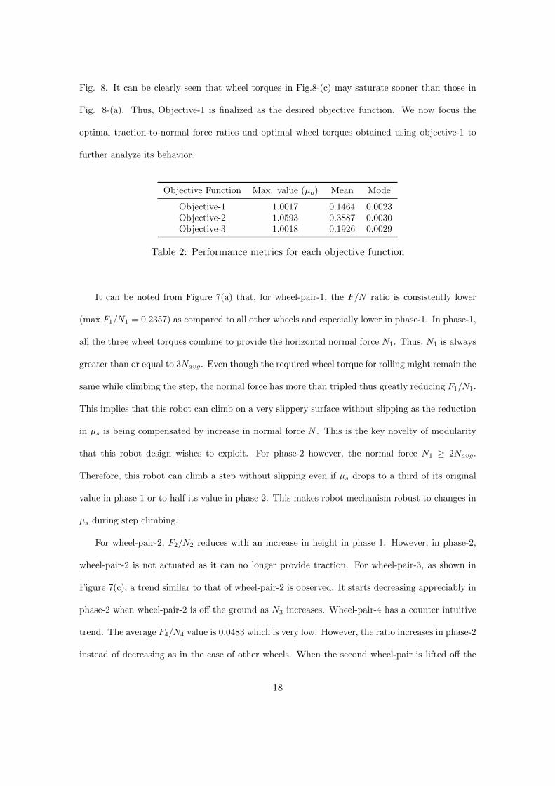
Fig. 8. It can be clearly seen that wheel torques in Fig.8-(c) may saturate sooner than those in

Fig. 8-(a). Thus, Objective-1 is finalized as the desired objective function. We now focus the

optimal traction-to-normal force ratios and optimal wheel torques obtained using objective-1 to

further analyze its behavior.

Objective Function Max. value (µo) Mean Mode

Objective-1 1.0017 0.1464 0.0023Objective-2 1.0593 0.3887 0.0030Objective-3 1.0018 0.1926 0.0029

Table 2: Performance metrics for each objective function

It can be noted from Figure 7(a) that, for wheel-pair-1, the F/N ratio is consistently lower

(max F1/N1 = 0.2357) as compared to all other wheels and especially lower in phase-1. In phase-1,

all the three wheel torques combine to provide the horizontal normal force N1. Thus, N1 is always

greater than or equal to 3Navg. Even though the required wheel torque for rolling might remain the

same while climbing the step, the normal force has more than tripled thus greatly reducing F1/N1.

This implies that this robot can climb on a very slippery surface without slipping as the reduction

in µs is being compensated by increase in normal force N . This is the key novelty of modularity

that this robot design wishes to exploit. For phase-2 however, the normal force N1 ≥ 2Navg.

Therefore, this robot can climb a step without slipping even if µs drops to a third of its original

value in phase-1 or to half its value in phase-2. This makes robot mechanism robust to changes in

µs during step climbing.

For wheel-pair-2, F2/N2 reduces with an increase in height in phase 1. However, in phase-2,

wheel-pair-2 is not actuated as it can no longer provide traction. For wheel-pair-3, as shown in

Figure 7(c), a trend similar to that of wheel-pair-2 is observed. It starts decreasing appreciably in

phase-2 when wheel-pair-2 is off the ground as N3 increases. Wheel-pair-4 has a counter intuitive

trend. The average F4/N4 value is 0.0483 which is very low. However, the ratio increases in phase-2

instead of decreasing as in the case of other wheels. When the second wheel-pair is lifted off the

18

ground, to maintain static equilibrium in the x-direction, forces are redistributed thus increasing

the values of F3 and F4. However, for wheel-pair-3, N3 also increases accordingly and therefore the

ratio could be kept lower. The normal force N4, on the other hand, doesn’t increase proportionally

thus increasing the ratio in the case of wheel-pair-4.

0 0.05 0.1 0.15 0.2 0.25 0.30

0.1

0.2

0.3

0.4

0.5

0.6

0.7

0.8

0.9

1 Wheel torques v/s height

Step height (m)

Wheel torque (Nm)

τw1

τw2

τw3

τw4

τwmax

(a)

0 0.05 0.1 0.15 0.2 0.25 0.30

0.1

0.2

0.3

0.4

0.5

0.6

0.7

0.8

0.9

1 Wheel torques v/s height

Step height (m)

Wheel torque (Nm)

(b)

0 0.05 0.1 0.15 0.2 0.25 0.30

0.1

0.2

0.3

0.4

0.5

0.6

0.7

0.8

0.9

1 Wheel torques v/s height

Step height (m)

Wheel torque (Nm)

τw1

τw2

τw3

τw4

τwmax

(c)

Figure 8: Optimal wheel torque plots for all the wheel pairs with a) objective function-1,b) objective function-2 and c) objective function-3

Note that, during phase-1, F1/N1 = 0 and F4/N4 = 0. This implies that, in the optimal case,

wheel-pairs-1 and -4 don’t apply any traction to maintain static-stability. In effect, wheel-pairs-

1 and -4 are simply rolled along without needing any actuation. As the robot begins to climb

up, wheel-pair-1 loses its normal force in the vertical direction and subsequently N2 goes up to

do weight balance. Therefore, intuitively, the objective function is keeping the F/N values low

by driving F1 to zero and making wheel-pair-2 (thus F2) take the additional load. Since, wheel-

19

pair-4 normal force gets least effected during this process, F4/N4 is minimized by driving F4 to

zero. Therefore, in phase-1, wheel-pairs-2 and -3 play a major role in maintaining static balance.

However, in phase-2, wheel-pair-2 is lifted off the ground and this forces wheel-pairs-1 and -4 to

start exerting least possible force to maintain static balance while keeping their respective F/N

ratios low.

Fig. 8(a) shows the corresponding desired wheel torque values for all wheel-pairs obtained

using Objective-1. Note that, the torque values are quite low in phase-2 as compared to phase-1.

This is attributed to spring action. In phase-1, a part of the wheel-traction generated was used to

balance the resisting moment generated by the spring. However, in phase-2, the spring deformation

is much lower. Additionally, in spite of their low values, the moments due to N1 and F1 are high

enough to balance moments due to weight at J2 as the moment arm length increased significantly.

The optimal wheel torques obtained so far only maintain the robot in static equilibrium at a

given height. However, the robot has to be imparted with some motion to move from one set-

point to another. Additional torque needs to be applied to move the robot with a desired velocity.

Therefore, a velocity controller is coupled to these optimal wheel to obtain the desired optimal

wheel torque controller as described in the next section.

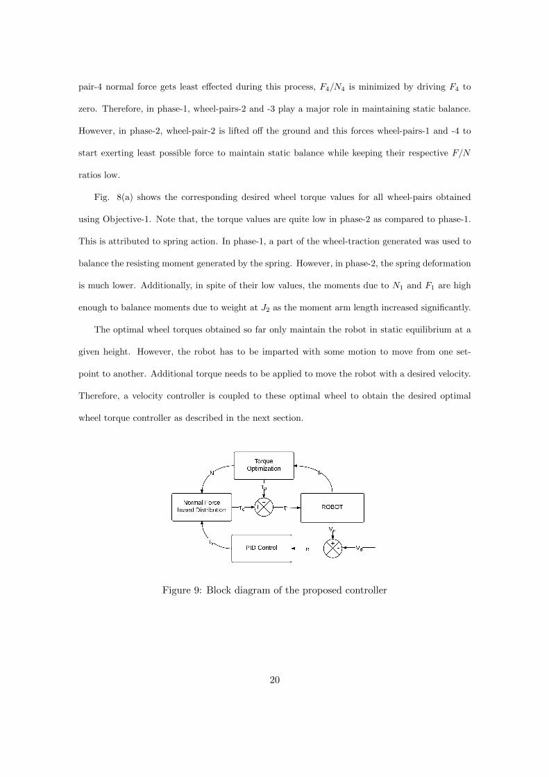
Figure 9: Block diagram of the proposed controller

20

5 Proposed Wheel Torque Controller Design

Optimal wheel-torque control is a very active research area and several instances of successful

application of wheel-torque control for mobile robots, like SHRIMP [11] and CRAB [6], have been

reported earlier in [4], [5], [7], [8]. A detailed study of this method is given in [12].

The discrete optimal-wheel torque values obtained from the previous section are fitted using

cubic splines such that they can be approximately estimated for any arbitrary value of θ1. For the

height that the robot climbed during the experiments, the robot’s state can be quite accurately

determined using θ1. The implementation details will be discussed in the next sub-section. In this

manner, the optimal-torque values are determined at every time-step and supplied to the robot in

an open-loop. While this maintains static stability at any given time-step, the robot needs to be

imparted some velocity to traverse from one state to another. To this end, a desired velocity, Vd,

is chosen. Accordingly, a velocity PD controller is developed. The torques required to maintain

static-stability (optimal-wheel torques) and to maintain speed are then added and supplied to the

robot. This combination will be referred to as torque controller, hereafter. This velocity control

loop ensures that the robot never gets stuck in a statically stable configuration, during the step

ascent. The block diagram of the proposed controller is shown in Fig. 9, where s denotes the

state of the robot , Vm and Vd denote the measured and desired wheel velocities, e denotes the

velocity error term, and τo, τv and τc denote the torque values obtained from the optimizer, velocity

controller, and torque scaled according to normal force, respectively.

It is worth noting that the normal forces (N) are used to augment the application of τv to all

the wheels, as shown in Fig. 9. Sometimes, PD controller commands high torques to quickly reach

a desired speed value. However, if the normal force at the wheel at that moment is very low, it

will cause the wheel to slip, while reaching the desired velocity. To minimize this problem, the

desired τv’s are scaled down based on the normal force values at that state, as obtained from the

optimization procedure. This way, the wheels can apply a higher fraction of τv when the normal

forces are higher too. This also ensures that τvi = 0 when the ith wheel loses contact with the

21

ground, thus saving energy. In Fig. 9, τc denotes the corrected torque for each individual wheel for

achieving the desired velocity. Note that, while this process may slow down a wheel from achieving

the desired velocity, it still achieves the larger goal of generating forward motion with minimal slip.

5.1 Numerical and Experimental Results

Two key metrics were used to study the performance of the robot. They are average slip ratio(sa)

and mean wheel-torque (T ). Slip ratio is given by, 1− v/rω, where v is the linear velocity of each

wheel and ω is the angular velocity measured by wheel encoder. The slip ratios of all the wheels

were determined and averaged to obtain the Average Slip Ratio. Similarly, the wheel-torques for

all the wheels were measured and averaged to obtain the Mean wheel-torque T .

The utility of the proposed torque control was compared to the conventional velocity control,

and the net reduction in slip ratio and torque requirement were estimated. Numerical experiments

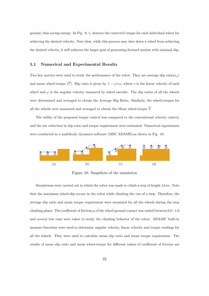
were conducted in a multibody dynamics software (MSC ADAMS),as shown in Fig. 10.

(a) (b) (c) (d)

Figure 10: Snapshots of the simulation

Simulations were carried out in which the robot was made to climb a step of height 14cm. Note

that the maximum wheel-slip occurs in the robot while climbing the rise of a step. Therefore, the

average slip ratio and mean torque requirement were measured for all the wheels during the step

climbing phase. The coefficient of friction µ of the wheel-ground contact was varied between 0.6−1.0

and several test runs were taken to study the climbing behavior of the robot. ADAMS’ built-in

measure functions were used to determine angular velocity, linear velocity and torque readings for

all the wheels. They were used to calculate mean slip ratio and mean torque requirement. The

results of mean slip ratio and mean wheel-torque for different values of coefficient of friction are

22

0.5 0.6 0.7 0.8 0.9 10.02

0.025

0.03

0.035

0.04

0.045

0.05

Coefficient of friction

Average Slip Ratio

Velocity Control

Torque Control

(a)

0.5 0.6 0.7 0.8 0.9 10.07

0.072

0.074

0.076

0.078

0.08

0.082

0.084

0.086

0.088

Coefficient of friction

Mean Torque (N)

Velocity Control

Torque Control

(b)

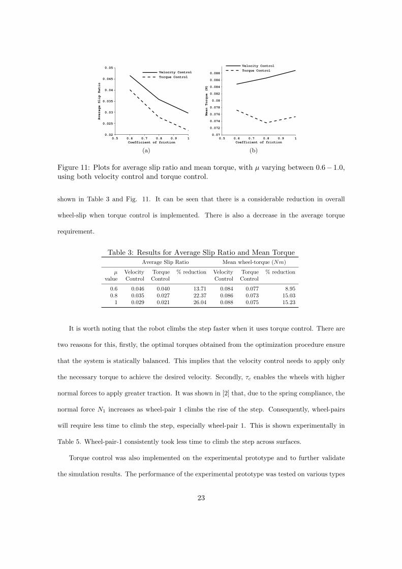
Figure 11: Plots for average slip ratio and mean torque, with µ varying between 0.6− 1.0,using both velocity control and torque control.

shown in Table 3 and Fig. 11. It can be seen that there is a considerable reduction in overall

wheel-slip when torque control is implemented. There is also a decrease in the average torque

requirement.

Table 3: Results for Average Slip Ratio and Mean TorqueAverage Slip Ratio Mean wheel-torque (Nm)

µ Velocity Torque % reduction Velocity Torque % reductionvalue Control Control Control Control

0.6 0.046 0.040 13.71 0.084 0.077 8.950.8 0.035 0.027 22.37 0.086 0.073 15.03

1 0.029 0.021 26.04 0.088 0.075 15.23

It is worth noting that the robot climbs the step faster when it uses torque control. There are

two reasons for this, firstly, the optimal torques obtained from the optimization procedure ensure

that the system is statically balanced. This implies that the velocity control needs to apply only

the necessary torque to achieve the desired velocity. Secondly, τc enables the wheels with higher

normal forces to apply greater traction. It was shown in [2] that, due to the spring compliance, the

normal force N1 increases as wheel-pair 1 climbs the rise of the step. Consequently, wheel-pairs

will require less time to climb the step, especially wheel-pair 1. This is shown experimentally in

Table 5. Wheel-pair-1 consistently took less time to climb the step across surfaces.

Torque control was also implemented on the experimental prototype and to further validate

the simulation results. The performance of the experimental prototype was tested on various types

23

Figure 12: Snapshots of the robot climbing, a 30 cm high step

Figure 13: Snapshots of the robot climbing the tiled floor.

of wheel-ground interfaces. It was made to climb a step of height 14 cm. It was previously shown

in [2] that the robot can climb steps upto 17 cm height. Infact, it can climb a step riser which is as

high as 30 cm without tipping over, as shown in Fig. 12. However, for the experiments conducted

in this paper, a relatively lower height if 14 cm is chosen. Note that, the focus of this paper is to

test and verify the utility of wheel-torque optimization in slip reduction for a robot whose climbing

ability has already been discussed and documented. Secondly, 14 cm is specifically chosen as it

roughly equals the height of a step-riser in residential stairways. The proposed compliant robot is

being altered to climb stairs and having this torque controller would not only make climbing more

energy efficient but also make wheel odometry more accurate.

Each link of the robot is fitted with an IMU sensor to accurately estimate it angle θi. The

IMU readings obtained from the first link are sent to the torque controller to estimate optimal

torque. The controller is implemented on a custom designed AtMega64 board. The robot was run

on 4 types of surfaces namely, tiled, carpeted, taped and wet, as shown in Fig.14(a)-(d). Snapshots

of the robot climbing the obstacle from a tiled floor are shown in Fig.13. The average slip ratio

and mean torque values obtained for all surfaces are tabulated in Table 4. Angular velocities of

individual wheels were noted using a wheel encoders. Starting and stopping points were marked

for all the wheels. The fixed distance travelled by the wheels was timed and linear velocities were

estimated from this data. Slip-ratio for each wheel can be calculated as σi = 1− vi/rωi, where v

24

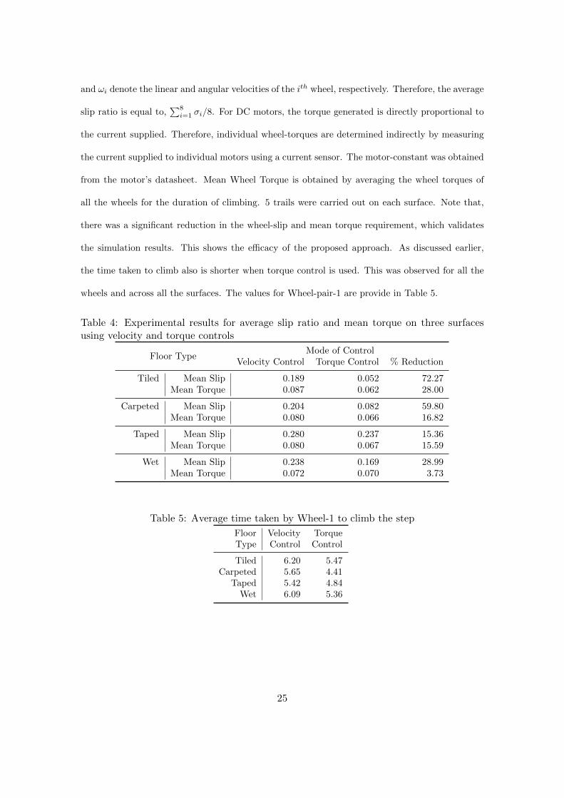
and ωi denote the linear and angular velocities of the ith wheel, respectively. Therefore, the average

slip ratio is equal to,∑8i=1 σi/8. For DC motors, the torque generated is directly proportional to

the current supplied. Therefore, individual wheel-torques are determined indirectly by measuring

the current supplied to individual motors using a current sensor. The motor-constant was obtained

from the motor’s datasheet. Mean Wheel Torque is obtained by averaging the wheel torques of

all the wheels for the duration of climbing. 5 trails were carried out on each surface. Note that,

there was a significant reduction in the wheel-slip and mean torque requirement, which validates

the simulation results. This shows the efficacy of the proposed approach. As discussed earlier,

the time taken to climb also is shorter when torque control is used. This was observed for all the

wheels and across all the surfaces. The values for Wheel-pair-1 are provide in Table 5.

Table 4: Experimental results for average slip ratio and mean torque on three surfacesusing velocity and torque controls

Floor TypeMode of Control

Velocity Control Torque Control % Reduction

Tiled Mean Slip 0.189 0.052 72.27Mean Torque 0.087 0.062 28.00

Carpeted Mean Slip 0.204 0.082 59.80Mean Torque 0.080 0.066 16.82

Taped Mean Slip 0.280 0.237 15.36Mean Torque 0.080 0.067 15.59

Wet Mean Slip 0.238 0.169 28.99Mean Torque 0.072 0.070 3.73

Table 5: Average time taken by Wheel-1 to climb the step

Floor Velocity TorqueType Control Control

Tiled 6.20 5.47Carpeted 5.65 4.41

Taped 5.42 4.84Wet 6.09 5.36

25

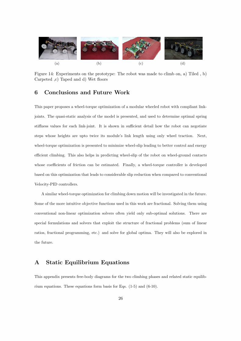
(a) (b) (c) (d)

Figure 14: Experiments on the prototype: The robot was made to climb on, a) Tiled , b)Carpeted ,c) Taped and d) Wet floors

6 Conclusions and Future Work

This paper proposes a wheel-torque optimization of a modular wheeled robot with compliant link-

joints. The quasi-static analysis of the model is presented, and used to determine optimal spring

stiffness values for each link-joint. It is shown in sufficient detail how the robot can negotiate

steps whose heights are upto twice its module’s link length using only wheel traction. Next,

wheel-torque optimization is presented to minimize wheel-slip leading to better control and energy

efficient climbing. This also helps in predicting wheel-slip of the robot on wheel-ground contacts

whose coefficients of friction can be estimated. Finally, a wheel-torque controller is developed

based on this optimization that leads to considerable slip reduction when compared to conventional

Velocity-PID controllers.

A similar wheel-torque optimization for climbing down motion will be investigated in the future.

Some of the more intuitive objective functions used in this work are fractional. Solving them using

conventional non-linear optimization solvers often yield only sub-optimal solutions. There are

special formulations and solvers that exploit the structure of fractional problems (sum of linear

ratios, fractional programming, etc.) and solve for global optima. They will also be explored in

the future.

A Static Equilibrium Equations

This appendix presents free-body diagrams for the two climbing phases and related static equilib-

rium equations. These equations form basis for Eqs. (1-5) and (6-10).

26

1. Free Body diagrams for the One Link Climbing Case

(a) Module 1

(a) Trunk 1 (b) Wheel 1

Figure 15:

For Wheel-1: ∑Fx = 0 : fxw1 −N1 = 0 (18)∑Fy = 0 : fyw1 − ww + F1 = 0 (19)∑

MW1= 0 : τw1 − F1r = 0 (20)

27

For Trunk-1: ∑Fx = 0 : fxl1 − fxw1 = 0 (21)∑Fy = 0 : fyl1 − wl − fyw1 = 0 (22)∑

MJ1 = 0 : k1φ1 + wl((l/2)cosφ1 − csinφ1) + fyw1lcosφ1

fxw1lsinφ1 − τw1 = 0 (23)

(b) Module 2

(a) Trunk 2 (b) Wheel 2

Figure 16:

For Wheel-2: ∑Fx = 0 : fxw2 − F2 = 0 (24)∑Fy = 0 : fyw2 −N2 + ww = 0 (25)∑

MW2= 0 : τw2 − F2r = 0 (26)

For Trunk-2:∑Fx = 0 : fxl2 − fxl1 + fxw2 = 0 (27)∑Fy = 0 : fyl2 + fyw2 − fyl1 − wl = 0 (28)∑

MJ2 = 0 : k2φ2 − k1φ1 + wl(l/2) + fyl1(l + l0)− fyw2l − τw2 = 0 (29)

28

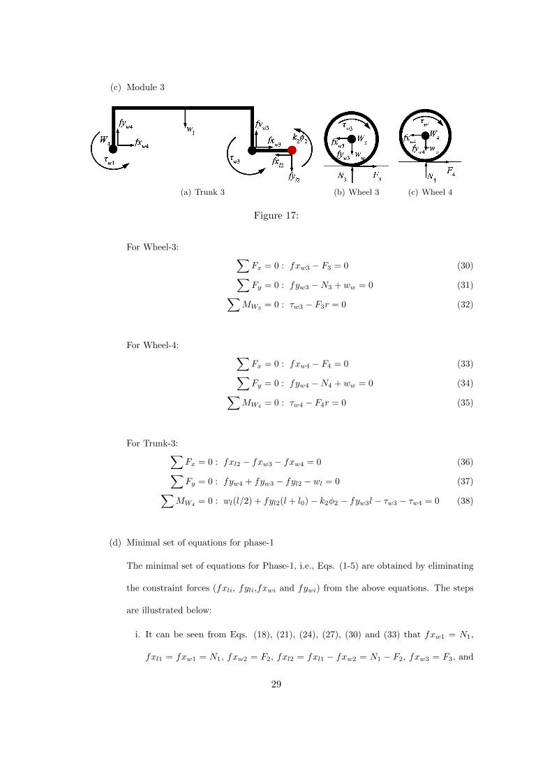
(c) Module 3

(a) Trunk 3 (b) Wheel 3 (c) Wheel 4

Figure 17:

For Wheel-3: ∑Fx = 0 : fxw3 − F3 = 0 (30)∑Fy = 0 : fyw3 −N3 + ww = 0 (31)∑

MW3= 0 : τw3 − F3r = 0 (32)

For Wheel-4: ∑Fx = 0 : fxw4 − F4 = 0 (33)∑Fy = 0 : fyw4 −N4 + ww = 0 (34)∑

MW4= 0 : τw4 − F4r = 0 (35)

For Trunk-3:∑Fx = 0 : fxl2 − fxw3 − fxw4 = 0 (36)∑Fy = 0 : fyw4 + fyw3 − fyl2 − wl = 0 (37)∑

MW4= 0 : wl(l/2) + fyl2(l + l0)− k2φ2 − fyw3l − τw3 − τw4 = 0 (38)

(d) Minimal set of equations for phase-1

The minimal set of equations for Phase-1, i.e., Eqs. (1-5) are obtained by eliminating

the constraint forces (fxli, fyli,fxwi and fywi) from the above equations. The steps

are illustrated below:

i. It can be seen from Eqs. (18), (21), (24), (27), (30) and (33) that fxw1 = N1,

fxl1 = fxw1 = N1, fxw2 = F2, fxl2 = fxl1 − fxw2 = N1 − F2, fxw3 = F3, and

29

fxw4 = F4, respectively. Therefore, Eq. (1) is obtained by substituting the values

fxl2, fxw3 and fxw4 from the above into (36).

ii. It can be seen from Eqs. (19), (22), (25), (28), (31) and (34) that fyw1 = ww−F1,

fyl1 = wl + fyw1 = wl +ww − F1, fyw2 = N2 −ww, fyl2 = −fyw2 + fyl1 +wl =

−N2 + 2ww + 2wl − F1, fyw3 = N3 − ww, and fyw4 = N4 − ww, respectively.

Hence, Eq. (2) is obtained by substituting the values fyw4, fyw3 and fyl2 from

the above into (37).

iii. Eq. (3) is obtained by substituting values of fxw1, fyw1 and τw1 from (18), (19)

and (20), respectively, into (23).

iv. Eq. (4) is obtained by substituting values of fyl1, fyw2, and τw2 from item − ii

above, (25) and (26), respectively, into (29).

v. Eq. (5) is obtained by substituting values of fyl2, fyw3, τw3 and τw4 from item−ii

above, (31), (32) and (35), respectively, into (38).

2. Free Body diagrams for the Two Link Climbing Case

(a) Module 1

(a) Trunk 1 (b) Wheel 1

Figure 18:

30

For Wheel-1: ∑Fx = 0 : fxw1 −N1 = 0 (39)∑Fy = 0 : fyw1 − ww + F1 = 0 (40)∑

MJ1 = 0 : τw1 − F1r = 0 (41)

For Trunk-1:∑Fx = 0 : fxl1 − fxw1 = 0 (42)∑Fy = 0 : fyl1 − wl − fyw1 = 0 (43)∑

MJ1 = 0 : k1φ1 + wl[(l/2)cos(φ1 + φ2)− csin(φ1 + φ2)] + fyw1lcos(φ1 + φ2)

− fxw1lsin(φ1 + φ2)− τw1 = 0 (44)

(b) Module 2

(a) Trunk 2 (b) Wheel 2

Figure 19:

For Wheel-2: ∑Fx = 0 : fxw2 = 0 (45)∑Fy = 0 : fyw2 + ww = 0 (46)∑

MJ1 = 0 : τw2 = 0 (47)

31

For Trunk-2:∑Fx = 0 : fxl2 − fxl1 + fxw2 = 0 (48)∑Fx = 0 : fyl2 + fyw2 − fyl1 − wl = 0 (49)∑

MJ1 = 0 : k2φ2 − k1φ1 + wl[(l/2)cosφ2 − csinφ2]

− fxl1(l + l0)sinφ2 + fyl1(l + l0)cosφ2 + fxw2lsinφ2 − fyw2lcosφ2 − τw2 = 0

(50)

(c) Module 3

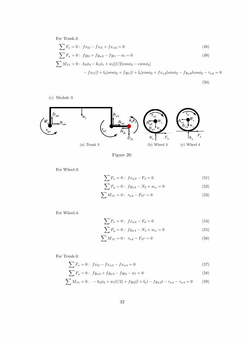
(a) Trunk 3 (b) Wheel 3 (c) Wheel 4

Figure 20:

For Wheel-3: ∑Fx = 0 : fxw3 − F3 = 0 (51)∑Fy = 0 : fyw3 −N3 + ww = 0 (52)∑

MJ1 = 0 : τw3 − F3r = 0 (53)

For Wheel-4: ∑Fx = 0 : fxw4 − F4 = 0 (54)∑Fy = 0 : fyw4 −N4 + ww = 0 (55)∑

MJ1 = 0 : τw4 − F4r = 0 (56)

For Trunk-3:∑Fx = 0 : fxl2 − fxw3 − fxw4 = 0 (57)∑Fy = 0 : fyw4 + fyw3 − fyl2 − wl = 0 (58)∑

MJ1 = 0 : − k2φ2 + wl(l/2) + fyl2(l + l0)− fyw3l − τw3 − τw4 = 0 (59)

32

(d) Minimal set of equations for phase-2

The minimal set of equations for Phase-2, i.e., Eqs. (6-10) are obtained by eliminating

the constraint forces (fxli, fyli,fxwi and fywi) from the above equations. The steps

are illustrated below:

i. It can be seen from Eqs. (39), (42), (45), (48), (51) and (54) that fxw1 = N1,

fxl1 = fxw1 = N1, fxw2 = 0, fxl2 = fxl1 − fxw2 = N1, fxw3 = F3, and

fxw4 = F4, respectively. Therefore, Eq. (6) is obtained by substituting the values

fxl2, fxw3 and fxw4 from the above into (57).

ii. It can be seen from Eqs. (40), (43), (46), (49), (52) and (55) that fyw1 = ww−F1 =

0, fyl1 = wl + fyw1 = wl + ww − F1, fyw2 = −ww, fyl2 = −fyw2 + fyl1 + wl =

2ww + 2wl −F1, fyw3 = N3 −ww, and fyw4 = N4 −ww, respectively. Hence, Eq.

(7) is obtained by substituting the values fyw4, fyw3 and fyl2 from the above into

(58).

iii. Eq. (8) is obtained by substituting values of fxw1, fyw1 and τw1 from (39), (40)

and (41), respectively, into (44).

iv. Eq. (9) is obtained by substituting values of fxl1, fyl1, fxw2, fyw2, and τw2 from

item− i above, item− ii above,(45), (46) and (47), respectively, into (50).

v. Eq. (10) is obtained by substituting values of fyl2, fyw3, τw3 and τw4 from item−ii

above, (52), (53) and (56), respectively, into (59).

References

[1] Dimitrios Apostolopoulos. Analytic configuration of wheeled robotic locomotion. 2001.

[2] Siravuru Avinash, Ankur Srivastava, Akshaya Purohit, Suril V Shah, and K Madhava Krishna.

A compliant multi-module robot for climbing big step-like obstacles. In IEEE International

Conference on Robotics and Automation (ICRA), Hong Kong, China, 2014.

33

[3] Siravuru Avinash, Suril V Shah, and K Madhava Krishna. Wheel torque optimization for a

compliant modular robot. In National Conference on Machines and Mechanisms (NaCoMM),

Roorkee, India, 2013.

[4] Pierre Lamon, Ambroise Krebs, Michel Lauria, Roland Siegwart, and Steven Shooter. Wheel

torque control for a rough terrain rover. In IEEE International Conference on Robotics and

Automation (ICRA), New Orleans, USA, 2004.

[5] P. Lamon and R. Siegwart. Wheel torque control in rough terrain-modeling and simulation.

In IEEE International Conference on Robotics and Automation (ICRA), Barcelona, Spain,

2005.

[6] Thomas Thueer, Pierre Lamon, Ambroise Krebs, and Roland Siegwart. Crab-exploration rover

with advanced obstacle negotiation capabilities. In Proceedings of the 9th ESA Workshop

on Advanced Space Technologies for Robotics and Automation (ASTRA), Noordwijk, The

Netherlands, 2006.

[7] Ambroise Krebs, Thomas Thueer, Edgar Carrasco, and Roland Siegwart. Towards torque

control of the crab rover. In Proceedings of the 9 th International Symposium on Artificial

Intelligence, Robotics and Automation in Space (iSAIRAS), Los Angeles, USA, 2008.

[8] Ambroise Krebs, Fabian Risch, Thomas Thueer, Jerome Maye, Cedric Pradalier, and Roland

Siegwart. Rover control based on an optimal torque distribution-application to 6 motorized

wheels passive rover. In IEEE/RSJ International Conference on Intelligent Robots and Sys-

tems (IROS), Taipei, Taiwan, 2010.

[9] Bin Xu, Cedric Pradalier, Ambroise Krebs, Roland Siegwart, and Fuchun Sun. Composite

control based on optimal torque control and adaptive kriging control for the crab rover. In

IEEE International Conference on Robotics and Automation (ICRA), Shanghai, China, 2011.

34

[10] K. Turker, I. Sharf, and M. Trentini. Step negotiation with wheel traction: a strategy for a

wheel-legged robot. In IEEE International Conference on Robotics and Automation (ICRA),

St. Paul, USA, 2012.

[11] T. Estier, Y. Crausaz, B. Merminod, M. Lauria, R. Piguet, and R. Siegwart. An innovative

space rover with extended climbing abilities. Proceedings of Space and Robotics, 2000:333–339,

2000.

[12] Ambroise Krebs, Thomas Thueer, Stephane Michaud, and Roland Siegwart. Performance op-

timization of all-terrain robots: a 2d quasi-static tool. In IEEE/RSJ International Conference

on Intelligent Robots and Systems (IROS), Beijing, China, 2006.

35