an optimal control approach to sequential machine teaching

An Optimal Control Approach to Sequential Machine Teaching

Laurent Lessard Xuezhou Zhang Xiaojin ZhuUniversity of Wisconsin–Madison University of Wisconsin–Madison University of Wisconsin–Madison

Abstract

Given a sequential learning algorithm anda target model, sequential machine teachingaims to find the shortest training sequenceto drive the learning algorithm to the targetmodel. We present the first principled wayto find such shortest training sequences. Ourkey insight is to formulate sequential machineteaching as a time-optimal control problem.This allows us to solve sequential teaching byleveraging key theoretical and computationaltools developed over the past 60 years in theoptimal control community. Specifically, westudy the Pontryagin Maximum Principle,which yields a necessary condition for opti-mality of a training sequence. We presentanalytic, structural, and numerical implica-tions of this approach on a case study witha least-squares loss function and gradient de-scent learner. We compute and visualize theoptimal training sequences for this problem,and find that they can vastly outperform thebest available heuristics for generating train-ing sequences.

1 INTRODUCTION

Machine teaching studies optimal control on machinelearners (Zhu et al., 2018; Zhu, 2015). In controls lan-guage the plant is the learner, the state is the modelestimate, and the input is the (not necessarily i.i.d.)training data. The controller wants to use the leastnumber of training items—a concept known as theteaching dimension (Goldman and Kearns, 1995)—toforce the learner to learn a target model. For exam-ple, in adversarial learning, an attacker may minimallypoison the training data to force a learner to learn a ne-farious model (Biggio et al., 2012; Mei and Zhu, 2015).

Proceedings of the 22nd International Conference on Ar-tificial Intelligence and Statistics (AISTATS) 2019, Naha,Okinawa, Japan. PMLR: Volume 89. Copyright 2019 bythe author(s).

Conversely, a defender may immunize the learner byinjecting adversarial training examples into the train-ing data (Goodfellow et al., 2014). In education sys-tems, a teacher may optimize the training curriculumto enhance student (modeled as a learning algorithm)learning (Sen et al., 2018; Patil et al., 2014).

Machine teaching problems are either batch or sequen-tial depending on the learner. The majority of priorwork studied batch machine teaching, where the con-troller performs one-step control by giving the batchlearner an input training set. Modern machine learn-ing, however, extensively employs sequential learningalgorithms. We thus study sequential machine teach-ing: what is the shortest training sequence to force alearner to go from an initial model w0 to some targetmodel w?? Formally, at time t = 0, 1, . . . the controllerchooses input (xt, yt) from an input set U . The learnerthen updates the model according to its learning algo-rithm. This forms a dynamical system f :

wt+1 = f(wt,xt, yt). (1a)

The controller has full knowledge of w0,w?, f,U , andwants to minimize the terminal time T subject towT = w?.

As a concrete example, we focus on teaching a gradientdescent learner of least squares:

f(wt,xt, yt) = wt − η(wTt xt − yt)xt (1b)

with w ∈ Rn and the input set ‖x‖ ≤ Rx, |y| ≤ Ry.We caution the reader not to trivialize the problem:(1) is a nonlinear dynamical system due to the inter-action between wt and xt. A previous best attemptto solve this control problem by Liu et al. (2017) em-ploys a greedy control policy, which at step t opti-mizes xt, yt to minimize the distance between wt+1

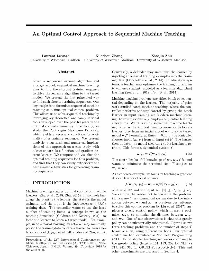
and w?. One of our observations is that this greedypolicy can be substantially suboptimal. Figure 1 showsthree teaching problems and the number of steps Tto arrive at w? using different methods. Our optimalcontrol method formulated as Nonlinear Programming(NLP) found shorter teaching sequences compared tothe greedy policy (lengths 151, 153, 259 for NLP vs219, 241, 310 for GREEDY, respectively). This andother experiments are discussed in Section 4.


0.0 0.5 1.0

0.0

0.2

0.4

0.6

0.8

1.0

GREEDY, T=219STRAIGHT, T=172NLP, T=151CNLP, tf =1.52s

−1 0 1

0.0

0.5

1.0

1.5

2.0

2.5

w0w ⋆GREEDY, T=241STRAIGHT, T=166NLP, T=153CNLP, tf =1.53s

−1 0 1

−1.0

−0.5

0.0

0.5

1.0

1.5

GREEDY, T=310STRAIGHT, T=305NLP, T=259CNLP, tf =2.59s

Figure 1: The shortest teaching trajectories found by different methods. All teaching tasks use the terminalpoint w? = (1, 0). The initial points used are w0 = (0, 1) (left panel), w0 = (0, 2.5) (middle panel), andw0 = (−1.5, 0.5) (right panel). The learner is the least squares gradient descent algorithm (1) with η = 0.01 andRx = Ry = 1. Total steps T to arrive at w? is indicated in the legends.

1.1 Main Contributions

Our main contribution is to show how tools from op-timal control theory may be brought to bear on themachine teaching problem. Specifically, we show that:

1. The Pontryagin optimality conditions reveal richstructural properties of the optimal teaching se-quences. Specifically, we provide a structuralcharacterization of solutions and show that, in theleast-squares case (1), the optimal solution alwayslies in a 2D subspace. These results are detailedin Section 3.

2. Optimal teaching sequences can be vastly moreefficient than what may be obtained via commonheuristics. We present two optimal approaches:an exact method (NLP) and a continuous approxi-mation (CNLP). Both agree when the stepsize η issmall, but CNLP is more scalable because its run-time does not depend on the length of the trainingsequence. These results are shown in Section 4.

We begin with a survey of the relevant optimal controltheory and algorithms literature in Section 2.

2 TIME-OPTIMAL CONTROL

To study the structure of optimal control we considerthe continuous gradient flow approximation of gradi-ent descent, which holds in the limit of diminishingstep size, i.e. η → 0. In this section, we present thecorresponding canonical time-optimal control problemand summarize some of the key theoretical and com-putational tools in optimal control that address it. Fora more detailed exposition on the theory, we refer thereader to modern references on the topic (Kirk, 2012;Liberzon, 2011; Athans and Falb, 2013).

This section is self-contained and we will use notationconsistent with the control literature (x instead of w,u instead of (x, y), tf instead of T ). We revert back tomachine learning notation in section 3. Consider thefollowing boundary value problem:

x = f(x, u) with x(0) = x0 and x(tf ) = xf . (2)

The function x : R+ → Rn is called the state andu : R+ → U is called the input. Here, U ⊆ Rm is agiven constraint set that characterizes admissible in-puts. The initial and terminal states x0 and xf arefixed, but the terminal time tf is free. If an admissibleu together with a state x satisfy the boundary valueproblem (2) for some choice of tf , we call (x, u) a tra-jectory of the system. The objective in a time-optimalcontrol problem is to find an optimal trajectory, whichis a trajectory that has minimal tf .

Established approaches for solving time-optimal con-trol problems can be grouped in three broad categories:dynamic programming, indirect methods, and directmethods. We now summarize each approach.

2.1 Dynamic Programming

Consider the value function V : Rn → R+, where V (x)is the minimum time required to reach xf startingat the initial state x. The Hamilton–Jacobi–Bellman(HJB) equation gives necessary and sufficient condi-tions for optimality and takes the form:

minu∈U

∇V (x)Tf(x, u) + 1 = 0 for all x ∈ Rn (3)

together with the boundary condition V (xf ) = 0. Ifthe solution to this differential equation is V?, then theoptimal input is given by the minimizer:

u(x) ∈ arg minu∈U

∇V?(x)Tf(x, u) for all x ∈ Rn (4)

Laurent Lessard, Xuezhou Zhang, Xiaojin Zhu

A nice feature of this solution is that the optimal inputu depends on the current state x. In other words, HJBproduces an optimal feedback policy.

Unfortunately, the HJB equation (3) is generally dif-ficult to solve. Even if the minimization has a closedform solution, the resulting differential equation is of-ten intractable. We remark that the optimal V? maynot be differentiable. For this reason, one looks forso-called viscosity solutions, as described by Liberzon(2011); Tonon et al. (2017) and references therein.

Numerical approaches for solving HJB include the fast-marching method (Tsitsiklis, 1995) and Lax–Friedrichssweeping (Kao et al., 2004). The latter reference alsocontains a detailed survey of other numerical schemes.

2.2 Indirect Methods

Also known as “optimize then discretize”, indirect ap-proaches start with necessary conditions for optimal-ity obtained via the Pontryagin Maximum Principle(PMP). The PMP may be stated and proved in sev-eral different ways, most notably using the Hamilto-nian formalism from physics or using the calculus ofvariations. Here is a formal statement.

Theorem 2.1 (PMP). Consider the boundary valueproblem (2) where f and its Jacobian with respect tox are continuous on Rn × U . Define the HamiltonianH : Rn × Rn × U → R as H(x, p, u) := pTf(x, u) + 1.If (x?, u?) is an optimal trajectory, then there existssome function p? : R+ → Rn (called the “co-state”)such that the following conditions hold.

a) x? and p? satisfy the following system of differen-tial equations for t ∈ [0, tf ] with boundary condi-tions x?(0) = x0 and x?(tf ) = xf .

x?(t) =∂H

∂p

(x?(t), p?(t), u?(t)

), (5a)

p?(t) = −∂H∂x

(x?(t), p?(t), u?(t)

). (5b)

b) For all t ∈ [0, tf ], an optimal input u?(t) satisfies:

u?(t) ∈ arg minu∈U

H(x?(t), p?(t), u). (6)

c) Zero Hamiltonian along optimal trajectories:

H(x?(t), p?(t), u?(t)) = 0 for all t ∈ [0, tf ]. (7)

In comparison to HJB, which needs to be solved for allx ∈ Rn, the PMP only applies along optimal trajecto-ries. Although the differential equations (5) may stillbe difficult to solve, they are simpler than the HJBequation and therefore tend to be more amenable toboth analytical and numerical approaches. Solutionsto HJB and PMP are related via ∇V ?(x?(t)) = p?(t).

PMP is only necessary for optimality, so solutionsof (5)–(7) are not necessarily optimal. Moreover, PMPdoes not produce a feedback policy; it only producesoptimal trajectory candidates. Nevertheless, PMP canprovide useful insight, as we will explore in Section 3.

If PMP cannot be solved analytically, a common nu-merical approach is the shooting method, where weguess p?(0), propagate the equations (5)–(6) forwardvia numerical integration. Then p?(0) is refined andthe process is repeated until the trajectory reaches xf .

2.3 Direct Methods

Also known as “discretize then optimize”, a sparsenonlinear program is solved, where the variables arethe state and input evaluated at a discrete set of time-points. An example is collocation methods, which usedifferent basis functions such as piecewise polynomi-als to interpolate the state between timepoints. Forcontemporary surveys of direct and indirect numericalapproaches, see Rao (2009); Betts (2010).

If the dynamics are already discrete as in (1), we maydirectly formulate a nonlinear program. We refer tothis approach as NLP. Alternatively, we can take thecontinuous limit and then discretize, which we callCNLP. We discuss the advantages and disadvantagesof both approaches in Section 4.

3 TEACHING LEAST SQUARES:INSIGHT FROM PONTRYAGIN

In this section, we specialize time-optimal control toleast squares. To recap, our goal is to find the mini-mum number of steps T such that there exists a controlsequence (xt, yt)0:T−1 that drives the learner (1) withinitial state w0 to the target state w?. The constraintset is U = {(x, y) | ‖x‖ ≤ Rx, |y| ≤ Ry}. This is annonlinear discrete-time time-optimal control problem,for which no closed-form solution is available.

On the corresponding continuous-time control prob-lem, applying Theorem 2.1 we obtain the followingnecessary conditions for optimality1 for all t ∈ [0, tf ].

w(0) = w0, w(tf ) = w? (8a)

w(t) =(y(t)−w(t)Tx(t)

)x(t) (8b)

p(t) =(p(t)Tx(t)

)x(t) (8c)

x(t), y(t) ∈ arg min‖x‖≤Rx, |y|≤Ry

(y −w(t)Tx

)(p(t)Tx) (8d)

0 =(y(t)−w(t)Tx(t)

)(p(t)Tx(t)

)+ 1 (8e)

1State, co-state, and input in Theorem 2.1 are (x, p, u),which is conventional controls notation. For this problem,we use (w,p, (x, y)), which is machine learning notation.


We can simplify (8) by setting y(t) = Ry, as describedin Proposition 3.1 below.

Proposition 3.1. For any trajectory (w,p,x, y) sat-isfying (8), there exist another trajectory of the form(w,p, x, Ry). So we may set y(t) = Ry without anyloss of generality.

Proof. Since (8d) is linear in y, the optimal y occursat a boundary and y = ±Ry. Changing the sign ofy is equivalent to changing the sign of x, so we mayassume without loss of generality that y = Ry. Thesechanges leave (8b)–(8c) and (8e) unchanged so w andp are unchanged as well.

In fact, Proposition 3.1 holds if we consider trajectoriesof (1) as well. For a proof, see the appendix.

Applying Proposition 3.1, the conditions (8d) and (8e)may be combined to yield the following quadraticallyconstrained quadratic program (QCQP) equation.

min‖x‖≤Rx

(Ry −wTx)(pTx) = −1 (9)

where we have omitted the explicit time specification(t) for clarity. Note that (9) constrains the possibletuples (w,p,x) that can occur as part of an optimaltrajectory. So in addition to solving the left-hand sideto find x, we must also ensure that it’s equal to−1. Wewill now characterize the solutions of (9) by examiningfive distinct regimes of the solution space that dependon the relationship between w and p as well as whichregime transitions are admissible.

Regime I (Origin): w = 0 and p 6= 0. This regimehappens when the teaching trajectory pass throughthe origin. In this regime, one can obtain closed-formsolutions. In particular, x = − Rx

‖p‖p and ‖p‖ = 1RxRy

.

In this regime, both w and p are positively alignedwith p. Therefore, Regime I necessarily transitionsfrom Regime II and into Regime III, given that it is notat the beginning or the end of the teaching trajectory.

Regime II (positive alignment): w = αp withp 6= 0 and α > 0. This regime happens when wand p are positively aligned. Again we have closedform solutions. In particular, x? = − Rx

‖w‖w and α =

Rx‖w‖(Ry+Rx‖w‖). In this regime, both w and p arenegatively aligned with w, thus Regime II necessarilytransitions into Regime I and can never transition fromany other regimes.

Regime III (negative alignment inside theorigin-centered ball): w = −αp with p 6= 0

and α > 0 and ‖w‖ ≤ Ry

2Rx. This regime happens

when w and p are negatively aligned and w is insidethe ball centered at the origin with radius R =

Ry

2Rx.

Again, closed form solutions exists: x? = Rx

‖w‖w and

α = R‖w‖(1 − R‖w‖). Regime III necessarily transi-tions from Regime I and into Regime IV.

Regime IV (negative alignment out of theorigin-centered ball): w = −αp with p 6= 0 and

α > 0 and ‖w‖ > Ry

2Rx. In this case, the solutions

satisfies α =R2

y

4 so that p is uniquely determined by w.However, the optimal x? is not unique. Any solutionto wTx =

Ry

2 with ‖x‖ ≤ Rx can be chosen. RegimeIV can only transition from Regime III and cannottransition into any other regime. In other word, oncethe teaching trajectory enters Regime IV, it cannotescape. Another interesting property of Regime IV isthat we know exactly how fast the norm of w is chang-ing. In particular, knowing wTx =

Ry

2 , one can derive

that d‖w‖2dt =

R2y

2 . As a result, once the trajectory en-ters regime IV, we know exact how long it will take forthe trajectory to reach w?, if it is able to reach it.

Regime V (general positions): w and p are lin-early independent. This case covers the remainingpossibilities for the state and co-state variables. Tocharacterize the solutions in this regime, we’ll first in-troduce some new coordinates. Define {w, u} to be theorthonormal basis for span{w,p} such that w = γwand p = αw + βu for some α, β, γ ∈ R. Note thatβ 6= 0 because we assume w and p are assumed tobe linearly independent in this regime. We can there-fore express any input uniquely as x = ww + uu + zzwhere z is an out-of-plane unit vector orthogonal toboth w and u, and w, u, z ∈ R are suitably chosen.Substituting these definitions, (9) becomes

minw2+u2+z2≤R2

x

(Ry − γw)(αw + βu) = −1. (10)

Now observe that the objective is linear in u and doesnot depend on z. The objective is linear in u be-cause β 6= 0 and (1 − γw) 6= 0 otherwise the entireobjective would be zero. Since the feasible set is con-vex, the optimal u must occur at the boundary of thefeasible set of variables w and u. Therefore, z = 0.This is profound, because it implies that in Regime V,the optimal solution necessarily lies on the 2D planespan{w,p}. In light of this fact, we can pick a moreconvenient parametrization. Let w = Rx cos θ andu = Rx sin θ. Equation (10) becomes:

minθ

Rx(Ry − γRx cos θ)(α cos θ + β sin θ) = −1. (11)

This objective function has at most four critical points,of which there is only one global minimum, and we canfind it numerically. Last but not least, Regime V doesnot transition from or into any other Regime.


III III IV V

w?

−1.0 −0.5 0.0 0.5 1.0 1.5

−0.2

0.0

0.2

0.4

0.6

0.8

1.0

1.2

1.4

I

II

III

IV

Vw?

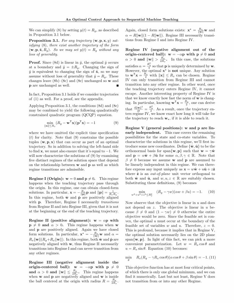
Figure 2: Optimal trajectories for w? = (1, 0) for dif-ferent choices of w0. Trajectories are colored accordingto the regime to which they belong and the directedgraph above shows all possible transitions. The opti-mal trajectories are symmetric about the x-axis. Forimplementation details, see Section 4.

Intrinsic low-dimensional structure of the opti-mal control solution. As is hinted in the analysisof Regime V, the optimal control x sometimes lies inthe 2D subspace spanned by w and p. In fact, thisholds not only for Regime V but for the whole prob-lem. In particular, we make the following observation.

Theorem 3.2. There always exists a global optimaltrajectory of (8) that lies in a 2D subspace of Rn.

The detailed proof can be found in the appendix. Animmediate consequence of Theorem 3.2 is that if w0

and w? are linearly independent, we only need to con-sider trajectories that are confined to the subspacespan{w0,w?}. When w0 and w? are aligned, trajecto-ries are still 2D, and any subspace containing w0 andw? is equivalent and arbitrary choice can be made.

This insight is extremely important because it enablesus to restrict our attention to 2D trajectories eventhough the dimensionality of the original problem (n)may be huge. This allows us to not only obtain a moreelegant and accurate solution in solving the necessarycondition induced by PMP, but also to parametrize di-rect and indirect approaches (see Sections 2.2 and 2.3)to solve this intrinsically 2D problem more efficiently.

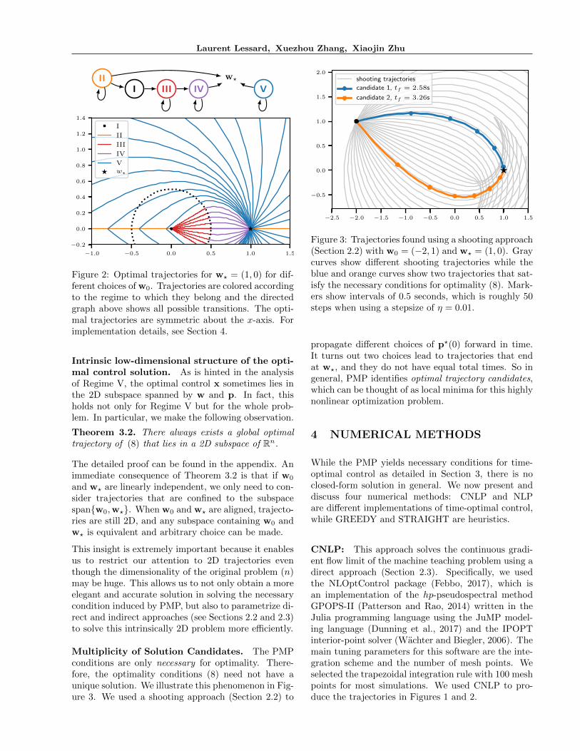
Multiplicity of Solution Candidates. The PMPconditions are only necessary for optimality. There-fore, the optimality conditions (8) need not have aunique solution. We illustrate this phenomenon in Fig-ure 3. We used a shooting approach (Section 2.2) to

−2.5 −2.0 −1.5 −1.0 −0.5 0.0 0.5 1.0 1.5

−0.5

0.0

0.5

1.0

1.5

2.0shooting trajectories

candidate 1, tf = 2.58s

candidate 2, tf = 3.26s

Figure 3: Trajectories found using a shooting approach(Section 2.2) with w0 = (−2, 1) and w? = (1, 0). Graycurves show different shooting trajectories while theblue and orange curves show two trajectories that sat-isfy the necessary conditions for optimality (8). Mark-ers show intervals of 0.5 seconds, which is roughly 50steps when using a stepsize of η = 0.01.

propagate different choices of p?(0) forward in time.It turns out two choices lead to trajectories that endat w?, and they do not have equal total times. So ingeneral, PMP identifies optimal trajectory candidates,which can be thought of as local minima for this highlynonlinear optimization problem.

4 NUMERICAL METHODS

While the PMP yields necessary conditions for time-optimal control as detailed in Section 3, there is noclosed-form solution in general. We now present anddiscuss four numerical methods: CNLP and NLPare different implementations of time-optimal control,while GREEDY and STRAIGHT are heuristics.

CNLP: This approach solves the continuous gradi-ent flow limit of the machine teaching problem using adirect approach (Section 2.3). Specifically, we usedthe NLOptControl package (Febbo, 2017), which isan implementation of the hp-pseudospectral methodGPOPS-II (Patterson and Rao, 2014) written in theJulia programming language using the JuMP model-ing language (Dunning et al., 2017) and the IPOPTinterior-point solver (Wachter and Biegler, 2006). Themain tuning parameters for this software are the inte-gration scheme and the number of mesh points. Weselected the trapezoidal integration rule with 100 meshpoints for most simulations. We used CNLP to pro-duce the trajectories in Figures 1 and 2.


NLP: A naıve approach to optimal control is to findthe minimum T for which there is a feasible inputsequence to drive the learner to w?. Fixing T , thefeasibility subproblem is a nonlinear program over 2Tn-dimensional variables x0, . . . ,xT−1 and w1, . . . ,wT

constrained by learner dynamics. Recall w0 is given,and one can fix yt = Ry for all t by Proposition 3.1.For our learner (1), the feasibility problem is

minw1:T ,x0:T−1

0 (12)

s.t. wT = w?

wt+1 = wt − η(wTt xt −Ry)xt

‖xt‖ ≤ Rx, ∀t = 0, . . . , T − 1.

As in the CNLP case, we modeled and solved the sub-problems (12) using JuMP and IPOPT. We also triedKnitro, a state-of-the-art commercial solver (Byrdet al., 2006), and it produced similar results. We stressthat such feasibility problems are difficult; IPOPT andKnitro can handle moderately sized T . For our spe-cific learner (1) there are 2D optimal control and statetrajectories in span{w0,w?} as discussed in Section 3.Therefore, we reparameterized (12) to work in 2D.

On top of this, we run a binary search over positiveintegers to find the minimum T for which the sub-problem (12) is feasible. Subject to solver numericalstability, the minimum T and its feasibility solutionx0, . . . ,xT−1 is the time-optimal control. While NLPis conceptually simple and correct, it requires solv-ing many subproblems with 2T variables and 2T con-straints, making it less stable and scalable than CNLP.

GREEDY: We restate the greedy control policy ini-tially proposed by Liu et al. (2017). It has the ad-vantage of being computationally more efficient andreadily applicable to different learning algorithms (i.e.dynamics). Specifically for the least squares learner (1)and given the current state wt, GREEDY solves thefollowing optimization problem to determine the nextteaching example (xt, yt):

min(xt,yt)∈U

‖wt+1 −w?‖2 (13)

s.t. wt+1 = wt − η(wTt xt − yt)xt.

The procedure repeats until wt+1 = w?. We usedthe Matlab function fmincon to solve the abovequadratic program iteratively. We point out that theoptimization problem is not convex. Moreover, wt+1

does not necessarily point in the direction of w?. Thisis evident in Figure 1 and Figure 6.

STRAIGHT: We describe an intuitive control pol-icy: at each step, move w in straight line toward w?

as far as possible subject to the constraint U . This

policy is less greedy than GREEDY because it maynot reduce ‖wt+1 −w?‖2 as much at each step. Theper-step optimization in x is a 1D line search:

mina,yt∈R

‖wt+1 −w?‖2 (14)

s.t. xt = a(w? −wt)/‖w? −wt‖(xt, yt) ∈ Uwt+1 = wt − η(wT

t xt − yt)xt.

The line search (14) can be solved in closed-form. Inparticular, one can obtain that

a =

{min{Rx, Ry‖w?−w‖

2(w?−w)Tw}, if (w? −w)Tw > 0

Rx, otherwise.

4.1 Comparison of Methods

We ran a number of experiments to study the behaviorof these numerical methods. In all experiments, thelearner is gradient descent on least squares (1), andthe control constraint set is ‖x‖ ≤ 1, |y| ≤ 1. Our firstobservation is that CNLP has a number of advantages:

1. CNLP’s continuous optimal state trajectorymatches NLP’s discrete state trajectories, espe-cially on learners with small η. This is expected,since the continuous optimal control problem isobtained asymptotically from the discrete one asη → 0. Figure 4 shows the teaching task w0 =(1, 0) ⇒ w∗ = (1, 0). Here we compare CNLPwith NLP’s optimal state trajectories on four gra-dient descent learners with different η values. TheNLP optimal teaching sequences vary drasticallyin length T , but their state trajectories quicklyoverlap with CNLP’s optimal trajectory.

2. CNLP is quick to compute, while NLP runtimegrows as the learner’s η decreases. Table 1presents the wall clock time. With a small η, theoptimal control takes more steps (larger T ). Con-sequently, NLP must solve a nonlinear programwith more variables and constraints. In contrast,CNLP’s runtime does not depend on η.

3. CNLP can be used to approximately compute the“teaching dimension”, i.e. the minimum num-ber of sequential teaching steps T for the discreteproblem. Recall CNLP produces an optimal ter-minal time tf . When the learner’s η is small,the discrete “teaching dimension” T is related byT ≈ tf/η. This is also supported by Table 1.

That said, it is not trivial to extract a discrete controlsequence from CNLP’s continuous control function.This hinders CNLP’s utility as an optimal teacher.


0.0 0.5 1.0

0.0

0.2

0.4

0.6

0.8

1.0

CNLP, tf =1.52sNLP, η=0.4, T=4NLP, η=0.02, T=76NLP, η=0.001, T=1515

−1 0 1

0.0

0.5

1.0

1.5

2.0

2.5

w0w ⋆CNLP, tf =1.53sNLP, η=0.4, T=4NLP, η=0.02, T=76NLP, η=0.001, T=1531

−1 0 1

−1.0

−0.5

0.0

0.5

1.0

1.5

CNLP, tf =2.59sNLP, η=0.4, T=6NLP, η=0.02, T=129NLP, η=0.001, T=2594

Figure 4: Comparison of CNLP vs NLP. All teaching tasks use the terminal point w? = (1, 0). The initial pointsused are w0 = (0, 1) (left panel), w0 = (0, 2.5) (middle panel), and w0 = (−1.5, 0.5) (right panel). We observethat the NLP trajectories on learners with smaller η’s quickly converges to the CNLP trajectory.

Table 1: Teaching sequence length and wall clock timecomparison. NLP teaches three learners with differentη’s. Target is always w? = (1, 0). All experimentswere performed on a conventional laptop.

NLP CNLPw0 η = 0.4 0.02 0.001

(0, 1) T = 3 75 1499 tf = 1.52s0.013s 0.14s 59.37s 4.1s

(0, 2.5) T = 5 76 1519 tf = 1.53s0.008s 0.11s 53.28s 2.37s

(−1.5, 0.5) T = 6 128 2570 tf = 2.59s0.012s 0.63s 310.08s 2.11s

Table 2: Comparison of teaching sequence length T .We fixed η = 0.01 in all cases.

w0 w? NLP STRAIGHT GREEDY

(0, 1) (2, 0) 148 161 233(0, 2) (4, 0) 221 330 721(0, 4) (8, 0) 292 867 2667(0, 8) (16, 0) 346 2849 10581

Our second observation is that NLP, being thediscrete-time optimal control, produces shorter teach-ing sequences than GREEDY or STRAIGHT. This isnot surprising, and we have already presented threeteaching tasks in Figure 1 where NLP has the small-est T . In fact, there exist teaching tasks on whichGREEDY and STRAIGHT can perform arbitrarilyworse than the optimal teaching sequence found byNLP. A case study is presented in Table 2. In this setof experiments, we set w0 = (a, 0) and w? = (0, 2a).As a increases, the ratio of teaching sequence lengthbetween STRAIGHT and NLP and between GREEDYand NLP grow at an exponential rate.

−0.5 0.0 0.5 1.0 1.5 2.0

−0.5

0.0

0.5

1.0

1.5

2.0

Figure 5: Points reachable in one step of gradient de-scent (with η = 0.1) on a least-squares objective start-ing from each of the black dots. There is circular sym-metry about the origin (red dot).

We now dig deeper and present an intuitive ex-planation of why GREEDY requires more teachingsteps than NLP. The fundamental issue is the non-linearity of the learner dynamics (1) in x. Forany w let us define the one-step reachable set{w − η(wTx− y)x

∣∣ (x, y) ∈ U}

. Figure 5 shows asample of such reachable sets. The key observationis that the starting w is quite close to the boundaryof most reachable sets. In other words, there is oftena compressed direction—from w to the closest bound-ary of U—along which w makes minimal progress. TheGREEDY scheme falls victim to this phenomenon.


0.0 0.5 1.0

0.0

0.5

1.0

NLP, T=14w0w⋆

0.0 0.5 1.0

GREEDY, T=21w0w ⋆

Figure 6: Reachable sets along the trajectory of NLP(left panel) and GREEDY (right panel). To minimizeclutter, we only show every 3rd reachable set. For thissimulation, we used η = 0.1. The greedy approachmakes fast progress initially, but slows down later on.

−1

0

GREEDY STRAIGHT

−1 0 1

−1

0

NLP

−1 0 1

CNLP

Figure 7: Trajectories of the input sequence {xt} forGREEDY, STRAIGHT, and NLP methods and thecorresponding x(t) for CNLP. The teaching task isw0 = (−1.5, 0.5), w? = (1, 0), and η = 0.01. Markersshow every 10 steps. Input constraint is ‖x‖ ≤ 1.

Figure 6 compares NLP and GREEDY on a teachingtask chosen to have short teaching sequences in orderto minimize clutter. GREEDY starts by eagerly de-scending a slope and indeed this quickly brings it closerto w?. Unfortunately, it also arrived at the x-axis. Forw on the x-axis, the compressed direction is horizon-tally outward. Therefore, subsequent GREEDY movesare relatively short, leading to a large number of stepsto reach w?. Interestingly, STRAIGHT is often bet-ter than GREEDY because it also avoids the x-axiscompressed direction for general w0.

We illustrate the optimal inputs in Figure 7, whichcompares {xt} produced by STRAIGHT, GREEDY,and NLP and the x(t) produced by CNLP. The heuris-tic approaches eventually take smaller-magnitudesteps as they approach w? while NLP and CNLP main-tain a maximal input norm the whole way.

5 CONCLUDING REMARKS

Techniques from optimal control are under-utilized inmachine teaching, yet they have the power to providebetter quality solutions as well as useful insight intotheir structure.

As seen in Section 3, optimal trajectories for the leastsquares learner are fundamentally 2D. Moreover, thereis a taxonomy of regimes that dictates their behavior.We also saw in Section 4 that the continuous CNLPsolver can provide a good approximation to the truediscrete trajectory when η is small. CNLP is also morescalable than simply solving the discrete NLP directlybecause NLP becomes computationally intractable asT gets large (or η gets small), whereas the runtime ofCNLP is independent of η.

A drawback of both NLP and CNLP is that they pro-duce trajectories rather than policies. In practice, us-ing an open-loop teaching sequence (xt, yt) will notyield the wt we expect due to the accumulation ofsmall numerical errors as we iterate. In order to find acontrol policy, which is a map from state wt to input(xt, yt), we discussed the possibility of solving HJB(Section 2.1) which is computationally expensive.

An alternative to solving HJB is to pre-compute thedesired trajectory via CNLP and then use model-predictive control (MPC) to find a policy that tracksthe reference trajectory as closely as possible. Suchan approach is used in Liniger et al. (2015), for ex-ample, to design controllers for autonomous race cars,and would be an interesting avenue of future work forthe machine teaching problem.

Finally, this paper presents only a glimpse at whatis possible using optimal control. For example, thePMP is not restricted to merely solving time-optimalcontrol problems. It is possible to analyze problemswith state- and input-dependent running costs, stateand input pointwise or integral constraints, conditionalconstraints, and even problems where the goal is toreach a target set rather than a target point.

Acknowledgements

We thank Ross Boczar and Max Simchoitz for helpfuldiscussions. This work is supported by NSF 1837132,1545481, 1704117, 1623605, 1561512, the MADLab AF


Center of Excellence FA9550-18-1-0166, and the Uni-versity of Wisconsin.

References

M. Athans and P. L. Falb. Optimal control: An intro-duction to the theory and its applications. CourierCorporation, 2013.

J. T. Betts. Practical methods for optimal control andestimation using nonlinear programming, volume 19.SIAM, 2010.

B. Biggio, B. Nelson, and P. Laskov. Poisoning attacksagainst support vector machines. In J. Langfordand J. Pineau, editors, 29th Int’l Conf. on MachineLearning (ICML). Omnipress, Omnipress, 2012.

R. H. Byrd, J. Nocedal, and R. A. Waltz. Knitro: Anintegrated package for nonlinear optimization. InLarge Scale Nonlinear Optimization, 35–59, 2006,pages 35–59. Springer Verlag, 2006.

I. Dunning, J. Huchette, and M. Lubin. Jump:A modeling language for mathematical optimiza-tion. SIAM Review, 59(2):295–320, 2017. doi:10.1137/15M1020575.

H. Febbo. Nloptcontrol.jl, 2017. URL :

https://github.com/JuliaMPC/NLOptControl.jl.

S. Goldman and M. Kearns. On the complexity ofteaching. Journal of Computer and Systems Sci-ences, 50(1):20–31, 1995.

I. J. Goodfellow, J. Shlens, and C. Szegedy. Explain-ing and Harnessing Adversarial Examples. ArXive-prints, Dec. 2014.

C. Y. Kao, S. Osher, and J. Qian. Lax–Friedrichssweeping scheme for static Hamilton–Jacobi equa-tions. Journal of Computational Physics, 196(1):367–391, 2004.

D. E. Kirk. Optimal control theory: An introduction.Courier Corporation, 2012.

D. Liberzon. Calculus of variations and optimal con-trol theory: A concise introduction. Princeton Uni-versity Press, 2011.

A. Liniger, A. Domahidi, and M. Morari.Optimization-based autonomous racing of 1:43scale RC cars. Optimal Control Applications andMethods, 36(5):628–647, 2015.

W. Liu, B. Dai, A. Humayun, C. Tay, C. Yu, L. B.Smith, J. M. Rehg, and L. Song. Iterative machineteaching. In International Conference on MachineLearning, pages 2149–2158, 2017.

S. Mei and X. Zhu. Using machine teaching to identifyoptimal training-set attacks on machine learners. InThe Twenty-Ninth AAAI Conference on ArtificialIntelligence, 2015.

K. Patil, X. Zhu, L. Kopec, and B. Love. Optimalteaching for limited-capacity human learners. InAdvances in Neural Information Processing Systems(NIPS), 2014.

M. A. Patterson and A. V. Rao. GPOPS-II: AMATLAB software for solving multiple-phase opti-mal control problems using hp-adaptive Gaussianquadrature collocation methods and sparse nonlin-ear programming. ACM Transactions on Mathemat-ical Software (TOMS), 41(1):1, 2014.

A. V. Rao. A survey of numerical methods for optimalcontrol. Advances in the Astronautical Sciences, 135(1):497–528, 2009.

A. Sen, P. Patel, M. A. Rau, B. Mason, R. Nowak,T. T. Rogers, and X. Zhu. Machine beats human atsequencing visuals for perceptual-fluency practice.In Educational Data Mining, 2018.

D. Tonon, M. S. Aronna, and D. Kalise. Optimal con-trol: Novel directions and applications, volume 2180.Springer, 2017.

J. N. Tsitsiklis. Efficient algorithms for globally opti-mal trajectories. IEEE Transactions on AutomaticControl, 40(9):1528–1538, 1995.

A. Wachter and L. T. Biegler. On the implementationof a primal-dual interior point filter line search algo-rithm for large-scale nonlinear programming. Math-ematical Programming, 106(1):25–57, 2006.

X. Zhu. Machine teaching: an inverse problem to ma-chine learning and an approach toward optimal ed-ucation. In The Twenty-Ninth AAAI Conferenceon Artificial Intelligence (AAAI “Blue Sky” SeniorMember Presentation Track), 2015.

X. Zhu, A. Singla, S. Zilles, and A. N. Rafferty. AnOverview of Machine Teaching. ArXiv e-prints, Jan.2018. https://arxiv.org/abs/1801.05927.

an optimal control approach to sequential machine teaching

Documents