an open-psa fault tree engine - arbre analystexfta-manual.pdf · xfta | an open-psa fault tree...
TRANSCRIPT
XFTA
October, 15th 2012
Antoine Rauzy
XFTA
An Open-PSA Fault Tree Engine
1
XFTA | An Open-PSA Fault Tree Engine
XFTAXFTAXFTAXFTA
An Open-PSA Fault Tree Engine
As we enter a time in which safety and reliability have come to the attention of the public, efforts are being made in the direction of the “next generation” of Probabilistic Safety Assessment (PSA) with regards to software and methods. These new initiatives hope to present a more informative view of the actual models of systems, components, and their interactions, which helps decision makers to go a step forward with their decisions.
The Open Initiative for Next Generation PSA (Open-PSA) provides an open and transparent public forum to disseminate information, independently review new ideas, and spread the word. We want to emphasize an openness which leads to methods and software which have better quality, better understanding and more flexibility, encourage peer review, and allow the transportability of models and methods.
We hope to bring to the international PSA community the benefits of an open initiative, and to bring together the different groups who engage in large scale PSA, in a non-competitive and commonly shared organization.
Fault Trees are probably the most widely used method for reliability and dependability studies. Fault Trees are recommended by most of Safety Standards and best practices. XFTA is a free calculation engine for Fault Trees described at the Open-PSA format.
2
XFTA | An Open-PSA Fault Tree Engine
TablTablTablTable of Contentse of Contentse of Contentse of Contents RELEASE NOTES ............................................................................................................... 3 INSTALLATION NOTES ........................................................................................................ 4
WINDOWS 7 (32 & 64 BITS) .............................................................................................. 4
LINUX (64 BITS) ............................................................................................................ 4
1 INTRODUCTION ........................................................................................................ 5 1.1 ORGANIZATION OF THE MANUAL............................................................................. 5
2 THE OPEN-PSA STANDARD .......................................................................................... 6
2.1 INTRODUCTORY EXAMPLE ..................................................................................... 6
2.2 FAULT TREE LAYER .............................................................................................. 8 2.3 STOCHASTIC LAYER ............................................................................................. 8
2.4 META-LOGICAL LAYER ....................................................................................... 10
2.4.1 COMMON CAUSE FAILURE GROUPS ................................................................. 10 2.4.2 DELETE TERMS & EXCHANGE EVENTS ............................................................... 10
3 SCRIPT FILES .......................................................................................................... 12
3.1 INTRODUCTORY EXAMPLE ................................................................................... 12
3.2 OPTIONS ........................................................................................................ 13 3.3 LOADING MODELS AND SCRIPTS ............................................................................ 14
3.4 OUTPUT FILES.................................................................................................. 14
3.5 PROBABILISTIC CALCULATIONS .............................................................................. 15 4 MINIMAL CUTSETS ................................................................................................... 16
4.1 COMPUTING MINIMAL CUTSETS ............................................................................ 16
4.2 PRINTING OUT MINIMAL CUTSETS .......................................................................... 17
5 IMPORTANCE FACTORS.............................................................................................. 18 5.1 TOP EVENT PROBABILITY AND CONDITIONAL PROBABILITIES .......................................... 18
5.2 MARGINAL IMPORTANCE FACTOR .......................................................................... 18
5.3 CRITICAL IMPORTANCE FACTOR ............................................................................ 18 5.4 DIAGNOSTIC IMPORTANCE FACTOR ........................................................................ 19
5.5 RISK ACHIEVEMENT WORTH ................................................................................ 19
5.6 RISK REDUCTION WORTH ................................................................................... 19
5.7 COMPUTING IMPORTANCE FACTORS ....................................................................... 19 6 SENSITIVITY ANALYSES ............................................................................................... 21
6.1 PRINCIPLE....................................................................................................... 21
6.2 DEFINITIONS.................................................................................................... 21 6.3 THE PSEUDO-RANDOM NUMBERS GENERATOR ............................................................ 22
6.4 PERFORMING SENSITIVITY ANALYSES ....................................................................... 22
7 SAFETY INTEGRITY LEVELS .......................................................................................... 24
7.1 MATHEMATICAL FOUNDATIONS ............................................................................ 24 7.2 DEFINITION OF SAFETY INTEGRITY LEVELS ................................................................ 26
7.3 EVALUATING SYSTEM UNAVAILABILITY THROUGH A PERIOD OF TIME ................................ 26
7.4 APPROXIMATING SYSTEM RELIABILITY BY MEANS OF FAILURE INTENSITY ............................. 28 8 KNOWN BUGS ........................................................................................................ 31
3
XFTA | An Open-PSA Fault Tree Engine
Release NotesRelease NotesRelease NotesRelease Notes The current version is 1.1. This is the second version to be released. It improves significantly the previous (1.0) version.
• The algorithm to calculate Minimal Custets has been improved by at different levels: preprocessing (more modules are captured), and in the algorithm itself (better variable selection heuristics, better data structures, better cutoff).
• The calculation of PFH has been simplified (it is now assimilated to the Unconditional Failure Intensity).
• A few bugs have been fixed.

4
XFTA | An Open-PSA Fault Tree Engine
Installation NotesInstallation NotesInstallation NotesInstallation Notes
Windows 7 (32 & 64 bits)Windows 7 (32 & 64 bits)Windows 7 (32 & 64 bits)Windows 7 (32 & 64 bits)
XFTA delivery consists of the following files.
• xfta.dll: the dynamic load library (DLL) that implements the XFTA interpreter.
• xftar.exe: the executable file that calls the DLL.
• xfta-api.h: the application programmable interface.
• xftar.cpp: the C++ source code for ‘xftar.exe”.
To install XFTA, you have to decompress the zip archive in any folder and to add to your environment variable PATH the path to that folder.
Once installed, to run XFTA on a script file “myscript.xml”, you have to open any command windows and to enter:
xftar.exe myscript.xml
While executing script file, XFTA prints out error messages on the standard error file (“stderr”). The default output file is the standard output file (“stdout”).
The Application Programmable Interface of XFTA is described in the file “xfta-api.h”. It is made of a single C function:
int XFTA_EvalScriptFile(char* fileName);
Calling this function executes the XFTA script file “filename”.
The source file “xftar.cpp” just loads the DLL “xfta.dll” and calls the function “XFTA_EvalScriptFile” on each argument of the command line. “xftar.cpp” is the source file for the executable “xftar.exe”.
LinuxLinuxLinuxLinux ((((64 bits64 bits64 bits64 bits ))))
XFTA delivery consists of the following file.
• xftar: the executable file that implements the XFTA interpreter
To install XFTA, you have to decompress the zip archive in any folder and to add to your environment variable PATH the path to that folder.
Once installed, to run XFTA on a script file “myscript.xml” you have to open any command windows and to enter:
xftar myscript.xml
While executing script file, XFTA prints out error messages on the standard error file (“stderr”). The default output file is the standard output file (“stdout”).

5
XFTA | An Open-PSA Fault Tree Engine
1111 IntroductionIntroductionIntroductionIntroduction XFTA is a Fault Tree calculation engine. XFTA takes a Fault Tree model at Open-PSA format as input and performs a number of calculations on that model. The model to be loaded and the calculations to be performed are described by means of XML files. Results are printed out into one or more text files (for most of the calculation results, these files are actually spreadsheets).
The current version of XFTA implements the so-called Fault Tree and stochastic layers of the Open-PSA format. It is therefore possible to describe Fault Trees with Basic Events, House Events, and Gate Events (with the usual connectives AND, OR, K/N, NOT…). Probability distributions can be associated with Basic Events. A whole menagerie of built-in failure models (Exponential, Weibull…), random deviates (uniform, normal, lognormal…) and user defined operations is available, just as in the Open-PSA format. Finally, several Common Cause Failure models are also available.
A typical XFTA session consists of the following steps:
• First, the model is loaded.
• Second, it is normalized, i.e. common cause failure models are expanded, constants are propagated…
• Third, Minimal Cutsets of the Top Event are calculated, for a given cutoff (maximum order and minimum probability of cutsets).
• Fourth, a number of probabilistic calculations are performed from the Minimal Cutsets.
The normalization step is transparent for the user: it is automatically invocated when the minimal cutsets calculation is launched. Moreover, it is fast (all operations it involves are of linear time complexity).
Minimal Cutsets calculation is by far the most resource consuming step, although the XFTA algorithm is a very efficient one.
Available probabilistic computations are the following:
• Top-Event probability.
• Importance Factors of Basic Events (Marginal Importance Factor, Critical Importance Factor, Diagnosis Importance Factor, Risk Achievement Worth, Risk Reduction Worth).
• Sensitivity Analysis by means of a Monte-Carlo simulation on the Top-Event Probability.
• Safety Integrity Levels for low demand and high demand system, as required by IEC 61508 and daughters standards.
1.11.11.11.1 Organization of the ManualOrganization of the ManualOrganization of the ManualOrganization of the Manual
The remainder of this manual is organized as follows.
• Section 2 presents briefly the part of the Open-PSA model exchange format XFTA implements.
• Section 3 introduces script files.
• Section 4 presents calculations of Minimal Cutsets.
• Section 5 presents calculations of Importance Factors.
• Section 6 presents Sensitivity Analyses.
• Section 7 presents calculations of Safety Integrity Levels.
• Finally, section 8 lists known bugs.
6
XFTA | An Open-PSA Fault Tree Engine
2222 The OpenThe OpenThe OpenThe Open----PSPSPSPSA StandardA StandardA StandardA Standard The Open-PSA standard is fully described in the following reference document.
Open-PSA Model Exchange Format. Steven Epstein & Antoine Rauzy Editors. The Open-PSA Initiative. Version 2.0d. April, 2008 (available at http://www.open-psa.org).
The present manual just describes which parts of the standard are implemented in XFTA, mainly by means of examples.
2.12.12.12.1 Introductory ExampleIntroductory ExampleIntroductory ExampleIntroductory Example
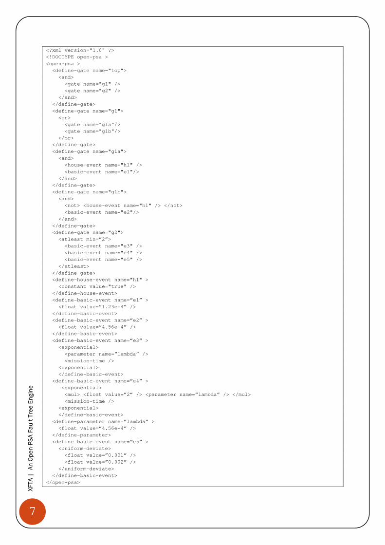
A model at the Open-PSA format is made of any number of XML files. It consists of Fault Trees and Event Trees. XFTA implements only the Fault Tree part of the standard. Moreover, only one Fault Tree can be loaded at a time. Therefore, a XFTA model consists of a number of declarations of gates, basic-events, house-events, parameters and CCF-group. An example of such a model is given on the next page.
In some document, the root tag of the XML file(s) is either ‘srf-psa’ or ‘opsa-mef’. XFTA accepts both, but ‘open-psa’ should be used preferably.
The structure function of the Fault Tree is made of a number of declarations of gates and house-events. These declarations can be gathered into a Fault Tree declaration for the sake of the compliancy with the full Open-PSA format. In our example, the model declares gates ‘top’, ‘g1’, ‘g1a’, ‘g1b’ and ‘g2’ and the house event ‘h1’. Note that the Boolean operator “atleast” corresponds to the so-called “k-out-of-n” of the Fault Tree literature (where the attribute “min” stands for “k” and “n” is kept implicit).
Probability distributions can be associated with basic events. The Open-PSA standard provides a wide set of arithmetic operators, built-in distributions and random deviates to do so.
In our example, basic events “e1” and “e2” are associated with constant distributions.
Distributions associated with basic events “e3” and “e4” are time dependent. It is defined by means of the “exponential” built-in, which corresponds to the Markovian assumption. The exponential distribution takes two
parameters: a failure rate λ and a mission time t. It is defined as follows.
exponential�, � = 1 − ���.� In our example, the parameter λ of the distribution associated with the basic event “e3” is a stochastic variable
named “lambda”, while the same parameter of the distribution associated with the basic event “e4” is twice the value of this variable. Stochastic variables are called “parameter” in the Open-PSA jargon. For both basic events, the mission time is the mission time of the system (which is set when a calculation is launched). It is possible to define as many stochastic variables as convenient. Expressions to define stochastic variables are the same as those to associated probability distributions to basic events.
The distribution associated with the basic event “e5” is random deviate. In this case, its value is uniformly distributed between 0.001 and 0.002. Random deviates are used to perform sensitivity analyses when the probability distributions of basic events are known only up to an uncertainty.
7
XFTA | An Open-PSA Fault Tree Engine
<?xml version="1.0" ?>
<!DOCTYPE open-psa >
<open-psa >
<define-gate name="top">
<and>
<gate name="g1" />
<gate name="g2" />
</and>
</define-gate>
<define-gate name="g1">
<or>
<gate name="g1a"/>
<gate name="g1b"/>
</or>
</define-gate>
<define-gate name="g1a">
<and>
<house-event name="h1" />
<basic-event name="e1"/>
</and>
</define-gate>
<define-gate name="g1b">
<and>
<not> <house-event name="h1" /> </not>
<basic-event name="e2"/>
</and>
</define-gate>
<define-gate name="g2">
<atleast min=”2”>
<basic-event name="e3" />
<basic-event name="e4" />
<basic-event name="e5" />
</atleast>
</define-gate>
<define-house-event name="h1" >
<constant value="true" />
</define-house-event>
<define-basic-event name=”e1” >
<float value=”1.23e-4” />
</define-basic-event>
<define-basic-event name=”e2” >
<float value=”4.56e-4” />
</define-basic-event>
<define-basic-event name=”e3” >
<exponential>
<parameter name=”lambda” />
<mission-time />
<exponential>
</define-basic-event>
<define-basic-event name=”e4” >
<exponential>
<mul> <float value=”2” /> <parameter name=”lambda” /> </mul>
<mission-time />
<exponential>
</define-basic-event>
<define-parameter name=”lambda” >
<float value=”4.56e-4” />
</define-parameter>
<define-basic-event name=”e5” >
<uniform-deviate>
<float value=”0.001” />
<float value=”0.002” />
</uniform-deviate>
</define-basic-event>
</open-psa>
8
XFTA | An Open-PSA Fault Tree Engine
2.22.22.22.2 Fault Tree layerFault Tree layerFault Tree layerFault Tree layer
The Fault Tree layer consists of the declarations of gates and house events, i.e. the structure function or the logical part of the Fault Tree.
XFTA identifiers for gates, house events, basic events, parameters and CCF groups are any printable ASCII string. Double quotes ‘”’, which are used to delimit XML attribute values, are not allowed.
XFTA implements connectives ‘and’, ‘or’, ‘atleast’ (k-out-of-n) and ‘not’. The standard proposes several other connectives1. However, most if not all Fault Tree models use only these four connectives.
Nothing prevents to use nested formulae (such as a ‘and’ of ‘or’ of events). However, a best practice recommended by all safety standards is to introduce an intermediary event per logical gate. The only exception to this rule is negations, as illustrated in our example. The compilation of Event Tree branches as well as the use of house events requires creating conjunctions of events and negations of events.
Gates and house events can be declared in any order, provided that there is no loop in the declarations (i.e. that an event depends eventually on itself).
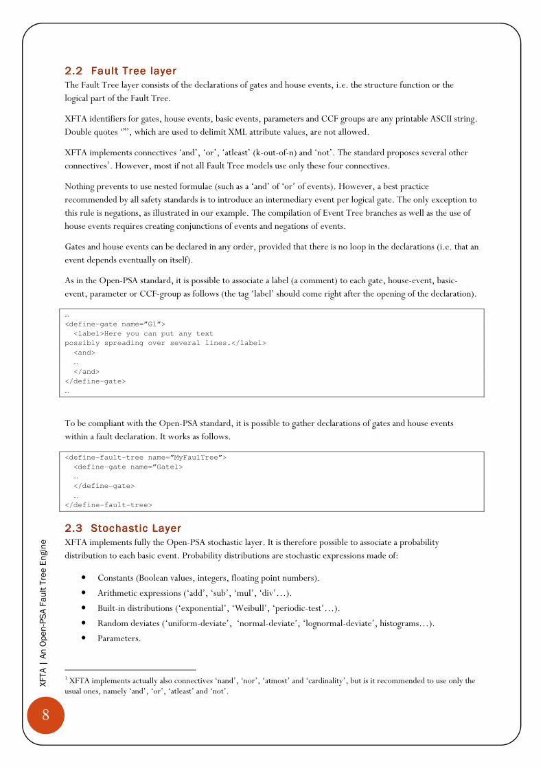
As in the Open-PSA standard, it is possible to associate a label (a comment) to each gate, house-event, basic-event, parameter or CCF-group as follows (the tag ‘label’ should come right after the opening of the declaration).
…
<define-gate name=”G1”>
<label>Here you can put any text
possibly spreading over several lines.</label>
<and>
…
</and>
</define-gate>
…
To be compliant with the Open-PSA standard, it is possible to gather declarations of gates and house events within a fault declaration. It works as follows.
<define-fault-tree name=”MyFaulTree”>
<define-gate name=”Gate1>
…
</define-gate>
…
</define-fault-tree>
2.32.32.32.3 Stochastic LayerStochastic LayerStochastic LayerStochastic Layer
XFTA implements fully the Open-PSA stochastic layer. It is therefore possible to associate a probability distribution to each basic event. Probability distributions are stochastic expressions made of:
• Constants (Boolean values, integers, floating point numbers).
• Arithmetic expressions (‘add’, ‘sub’, ‘mul’, ‘div’…).
• Built-in distributions (‘exponential’, ‘Weibull’, ‘periodic-test’…).
• Random deviates (‘uniform-deviate’, ‘normal-deviate’, ‘lognormal-deviate’, histograms…).
• Parameters.
1 XFTA implements actually also connectives ‘nand’, ‘nor’, ‘atmost’ and ‘cardinality’, but is it recommended to use only the usual ones, namely ‘and’, ‘or’, ‘atleast’ and ‘not’.
9
XFTA | An Open-PSA Fault Tree Engine
For a complete description of available stochastic constructs, refer to the Open-PSA reference document.
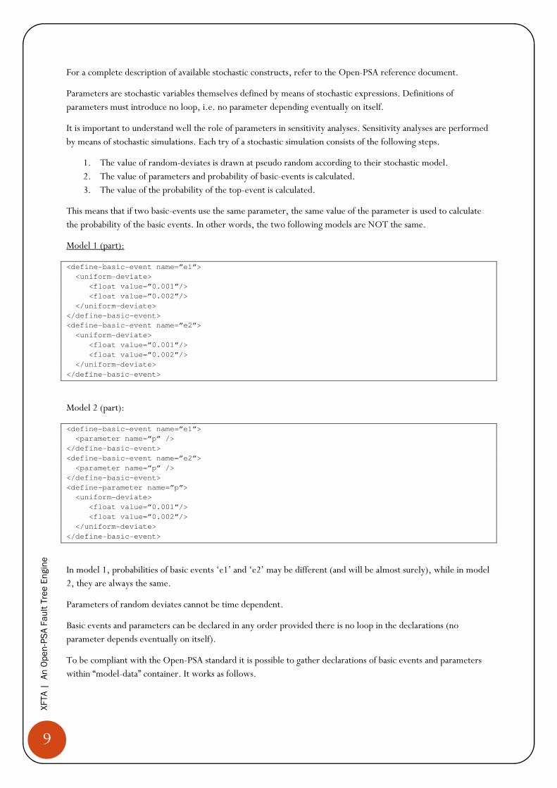
Parameters are stochastic variables themselves defined by means of stochastic expressions. Definitions of parameters must introduce no loop, i.e. no parameter depending eventually on itself.
It is important to understand well the role of parameters in sensitivity analyses. Sensitivity analyses are performed by means of stochastic simulations. Each try of a stochastic simulation consists of the following steps.
1. The value of random-deviates is drawn at pseudo random according to their stochastic model. 2. The value of parameters and probability of basic-events is calculated. 3. The value of the probability of the top-event is calculated.
This means that if two basic-events use the same parameter, the same value of the parameter is used to calculate the probability of the basic events. In other words, the two following models are NOT the same.
Model 1 (part):
<define-basic-event name=”e1”>
<uniform-deviate>
<float value=”0.001”/>
<float value=”0.002”/>
</uniform-deviate>
</define-basic-event>
<define-basic-event name=”e2”>
<uniform-deviate>
<float value=”0.001”/>
<float value=”0.002”/>
</uniform-deviate>
</define-basic-event>
Model 2 (part):
<define-basic-event name=”e1”>
<parameter name=”p” />
</define-basic-event>
<define-basic-event name=”e2”>
<parameter name=”p” />
</define-basic-event>
<define-parameter name=”p”>
<uniform-deviate>
<float value=”0.001”/>
<float value=”0.002”/>
</uniform-deviate>
</define-basic-event>
In model 1, probabilities of basic events ‘e1’ and ‘e2’ may be different (and will be almost surely), while in model 2, they are always the same.
Parameters of random deviates cannot be time dependent.
Basic events and parameters can be declared in any order provided there is no loop in the declarations (no parameter depends eventually on itself).
To be compliant with the Open-PSA standard it is possible to gather declarations of basic events and parameters within “model-data” container. It works as follows.
10
XFTA | An Open-PSA Fault Tree Engine
<model-data>
<define-basic-event name=”BE1”>
…
</define-basic-event>
…
</model-data>
2.42.42.42.4 MetaMetaMetaMeta ----Logical LayerLogical LayerLogical LayerLogical Layer
2.4.12.4.12.4.12.4.1 Common Cause Failure GroupsCommon Cause Failure GroupsCommon Cause Failure GroupsCommon Cause Failure Groups
XFTA implements the Common Cause Failure models proposed in the Open-PSA standard, namely:
• the Beta-factor model,
• the Multiple-Greek-Letter model,
• the Alpha-Factor model, and
• the Phi-factor model.
Before calculating minimal cutsets, the model is automatically normalized. One of the normalization operations consists in expanding CCF groups.
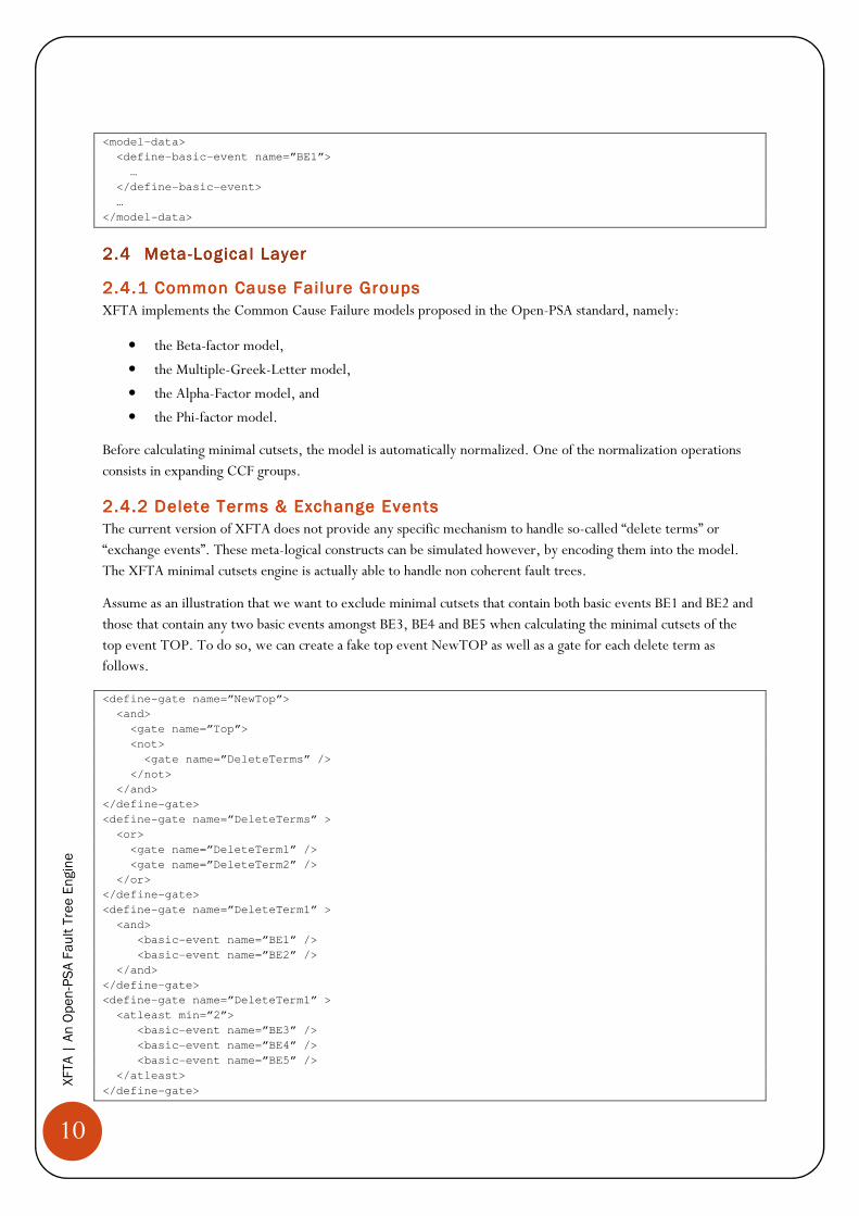
2.4.22.4.22.4.22.4.2 Delete TeDelete TeDelete TeDelete Terms & Exchange Eventsrms & Exchange Eventsrms & Exchange Eventsrms & Exchange Events
The current version of XFTA does not provide any specific mechanism to handle so-called “delete terms” or “exchange events”. These meta-logical constructs can be simulated however, by encoding them into the model. The XFTA minimal cutsets engine is actually able to handle non coherent fault trees.
Assume as an illustration that we want to exclude minimal cutsets that contain both basic events BE1 and BE2 and those that contain any two basic events amongst BE3, BE4 and BE5 when calculating the minimal cutsets of the top event TOP. To do so, we can create a fake top event NewTOP as well as a gate for each delete term as follows.
<define-gate name=”NewTop”>
<and>
<gate name=”Top”>
<not>
<gate name=”DeleteTerms” />
</not>
</and>
</define-gate>
<define-gate name=”DeleteTerms” >
<or>
<gate name=”DeleteTerm1” />
<gate name=”DeleteTerm2” />
</or>
</define-gate>
<define-gate name=”DeleteTerm1” >
<and>
<basic-event name=”BE1” />
<basic-event name=”BE2” />
</and>
</define-gate>
<define-gate name=”DeleteTerm1” >
<atleast min=”2”>
<basic-event name=”BE3” />
<basic-event name=”BE4” />
<basic-event name=”BE5” />
</atleast>
</define-gate>

11
XFTA | An Open-PSA Fault Tree Engine
12
XFTA | An Open-PSA Fault Tree Engine
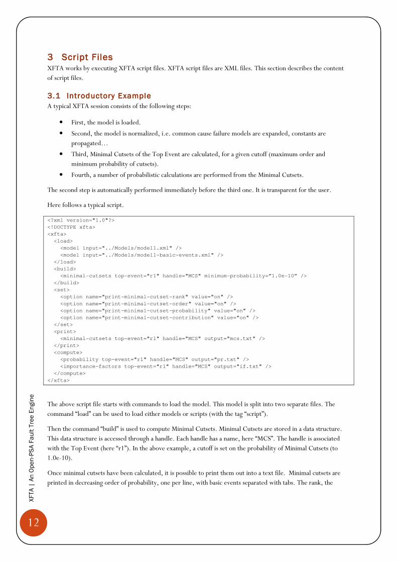
3333 Script FilesScript FilesScript FilesScript Files XFTA works by executing XFTA script files. XFTA script files are XML files. This section describes the content of script files.
3.13.13.13.1 Introductory ExampleIntroductory ExampleIntroductory ExampleIntroductory Example
A typical XFTA session consists of the following steps:
• First, the model is loaded.
• Second, the model is normalized, i.e. common cause failure models are expanded, constants are propagated…
• Third, Minimal Cutsets of the Top Event are calculated, for a given cutoff (maximum order and minimum probability of cutsets).
• Fourth, a number of probabilistic calculations are performed from the Minimal Cutsets.
The second step is automatically performed immediately before the third one. It is transparent for the user.
Here follows a typical script.
<?xml version="1.0"?>
<!DOCTYPE xfta>
<xfta>
<load>
<model input="../Models/model1.xml" />
<model input="../Models/model1-basic-events.xml" />
</load>
<build>
<minimal-cutsets top-event="r1" handle="MCS" minimum-probability=”1.0e-10” />
</build>
<set>
<option name="print-minimal-cutset-rank" value="on" />
<option name="print-minimal-cutset-order" value="on" />
<option name="print-minimal-cutset-probability" value="on" />
<option name="print-minimal-cutset-contribution" value="on" />
</set>
<print>
<minimal-cutsets top-event="r1" handle="MCS" output="mcs.txt" />
</print>
<compute>
<probability top-event="r1" handle="MCS" output="pr.txt" />
<importance-factors top-event="r1" handle="MCS" output="if.txt" />
</compute>
</xfta>
The above script file starts with commands to load the model. This model is split into two separate files. The command “load” can be used to load either models or scripts (with the tag “script”).
Then the command “build” is used to compute Minimal Cutsets. Minimal Cutsets are stored in a data structure. This data structure is accessed through a handle. Each handle has a name, here “MCS”. The handle is associated with the Top Event (here “r1”). In the above example, a cutoff is set on the probability of Minimal Cutsets (to 1.0e-10).
Once minimal cutsets have been calculated, it is possible to print them out into a text file. Minimal cutsets are printed in decreasing order of probability, one per line, with basic events separated with tabs. The rank, the
13
XFTA | An Open-PSA Fault Tree Engine
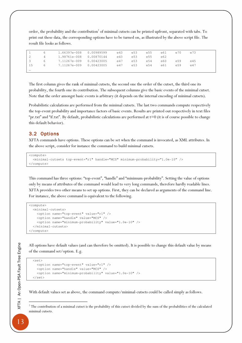
order, the probability and the contribution2 of minimal cutsets can be printed upfront, separated with tabs. To print out these data, the corresponding options have to be turned on, as illustrated by the above script file. The result file looks as follows.
1 6 1.66397e-008 0.00989599 e43 e53 e55 e61 e70 e73
2 4 1.98761e-008 0.00870144 e43 e53 e55 e62
3 6 7.11267e-009 0.00423005 e47 e53 e54 e60 e59 e45
15 6 7.11267e-009 0.00423005 e47 e53 e54 e61 e59 e47
…
The first column gives the rank of minimal cutsets, the second one the order of the cutset, the third one its probability, the fourth one its contribution. The subsequent columns give the basic events of the minimal cutset. Note that the order amongst basic events is arbitrary (it depends on the internal encoding of minimal cutsets).
Probabilistic calculations are performed from the minimal cutsets. The last two commands compute respectively the top-event probability and importance factors of basic events. Results are printed out respectively in text files “pr.txt” and “if.txt”. By default, probabilistic calculations are performed at t=0 (it is of course possible to change this default behavior).
3.23.23.23.2 OptionOptionOptionOptionssss
XFTA commands have options. These options can be set when the command is invocated, as XML attributes. In the above script, consider for instance the command to build minimal cutsets.
<compute>
<minimal-cutsets top-event="r1" handle="MCS" minimum-probability=”1.0e-10” />
</compute>
This command has three options: “top-event”, “handle” and “minimum-probability”. Setting the value of options only by means of attributes of the command would lead to very long commands, therefore hardly readable lines. XFTA provides two other means to set up options. First, they can be declared as arguments of the command line. For instance, the above command is equivalent to the following.
<compute>
<minimal-cutsets>
<option name="top-event" value="r1" />
<option name="handle" value="MCS" />
<option name="minimum-probability" value="1.0e-10" />
</minimal-cutsets>
</compute>
All options have default values (and can therefore be omitted). It is possible to change this default value by means of the command set/option. E.g.
<set>
<option name="top-event" value="r1" />
<option name="handle" value="MCS" />
<option name="minimum-probability" value="1.0e-10" />
</set>
With default values set as above, the command compute/minimal-cutsets could be called simply as follows.
2 The contribution of a minimal cutset is the probability of this cutset divided by the sum of the probabilities of the calculated minimal cutsets.
14
XFTA | An Open-PSA Fault Tree Engine
<compute>
<minimal-cutsets />
</compute>
Available options and their current values can be printed out by means of the following command.
<print>
<options output=”options.txt” />
</print>
The value of a particular option, e.g. “mission-time” can be printed out as follows.
<print>
<option name=”mission-time” output=”options.txt” />
</print>
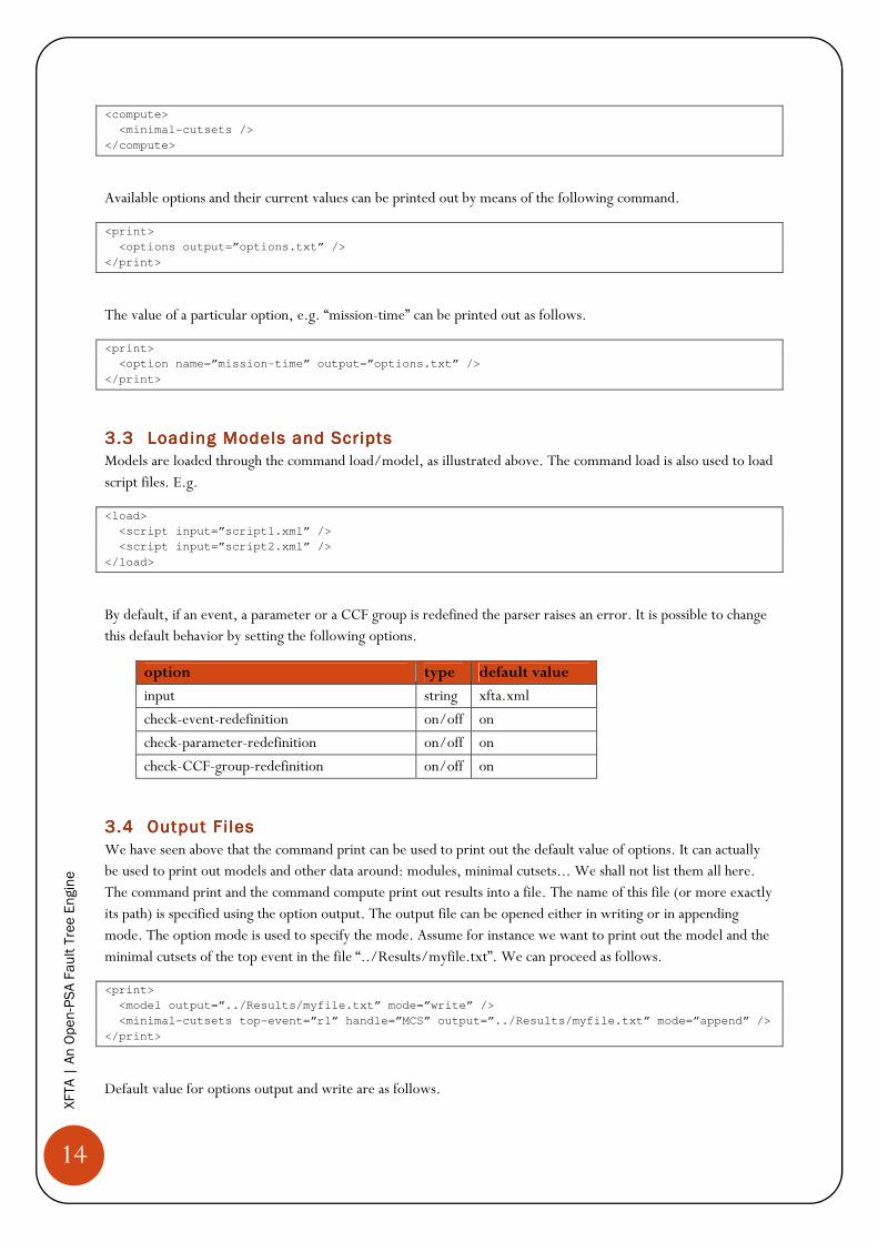
3.33.33.33.3 Loading Loading Loading Loading ModelModelModelModelssss and Scriptsand Scriptsand Scriptsand Scripts
Models are loaded through the command load/model, as illustrated above. The command load is also used to load script files. E.g.
<load>
<script input=”script1.xml” />
<script input=”script2.xml” />
</load>
By default, if an event, a parameter or a CCF group is redefined the parser raises an error. It is possible to change this default behavior by setting the following options.
option type default value
input string xfta.xml
check-event-redefinition on/off on
check-parameter-redefinition on/off on
check-CCF-group-redefinition on/off on
3.43.43.43.4 Output FilesOutput FilesOutput FilesOutput Files
We have seen above that the command print can be used to print out the default value of options. It can actually be used to print out models and other data around: modules, minimal cutsets... We shall not list them all here. The command print and the command compute print out results into a file. The name of this file (or more exactly its path) is specified using the option output. The output file can be opened either in writing or in appending mode. The option mode is used to specify the mode. Assume for instance we want to print out the model and the minimal cutsets of the top event in the file “../Results/myfile.txt”. We can proceed as follows.
<print>
<model output=”../Results/myfile.txt” mode=”write” />
<minimal-cutsets top-event=”r1” handle=”MCS” output=”../Results/myfile.txt” mode=”append” />
</print>
Default value for options output and write are as follows.
15
XFTA | An Open-PSA Fault Tree Engine
option type default value
output string result.txt
mode write/append write
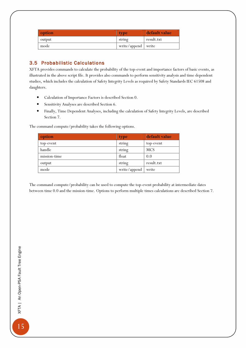
3.53.53.53.5 Probabil ist ic Calculat ionsProbabil ist ic Calculat ionsProbabil ist ic Calculat ionsProbabil ist ic Calculat ions
XFTA provides commands to calculate the probability of the top-event and importance factors of basic events, as illustrated in the above script file. It provides also commands to perform sensitivity analysis and time dependent studies, which includes the calculation of Safety Integrity Levels as required by Safety Standards IEC 61508 and daughters.
• Calculation of Importance Factors is described Section 0.
• Sensitivity Analyses are described Section 6.
• Finally, Time Dependent Analyses, including the calculation of Safety Integrity Levels, are described Section 7.
The command compute/probability takes the following options.
option type default value
top-event string top-event
handle string MCS
mission-time float 0.0
output string result.txt
mode write/append write
The command compute/probability can be used to compute the top-event probability at intermediate dates between time 0.0 and the mission-time. Options to perform multiple times calculations are described Section 7.
16
XFTA | An Open-PSA Fault Tree Engine
4444 Minimal CutsetsMinimal CutsetsMinimal CutsetsMinimal Cutsets In the current version of XFTA, all probabilistic calculations are performed on Minimal Cutsets (the future versions will probably implement Binary Diagram Calculations as well). The XTA algorithm to compute Minimal Cutsets is original. So is the data structure in which Minimal Cutsets are stored. Both are transparent for the user, up to the extent that the size of the resulting data structure is roughly proportional (in the worst case) to the number of Minimal Cutsets. Therefore, if you try to build a set of 123456789987654321 Minimal Cutsets, the running time and memory occupation will be proportional to 123456789987654321, which is indeed to avoid by any means. The current version of XFTA does not adjust the cutoff dynamically (this possibility will be probably provided in a future version). Therefore it is the user’s responsibility to set cutoffs so that calculations are not too resource consuming. Another very important feature of the XFTA algorithm is that it works for non-coherent fault trees, i.e. you can safely introduce negations in your model (as long as this has some physical meaning).
Note that the correct mathematical definition of Minimal Cutsets has been given for the first time in the following reference (long after this notion was in use):
A. Rauzy. Mathematical Foundations of Minimal Cutsets. IEEE Transactions on Reliability, volume 50,
number 4, pages 389-396,2001.
Loosely speaking a Cutset is a set of Basic Events such that if these Basic Events are realized (set to 1) and all other Basic Events are not (they are set to 0), then the Top Event is realized (it evaluates to 1). A Cutset is Minimal if none of its proper subsets is a Cutset.
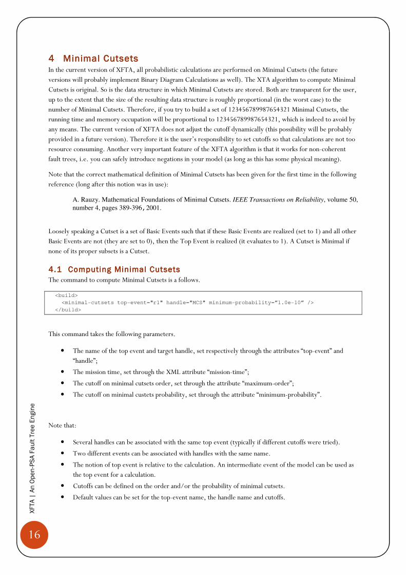
4.14.14.14.1 ComComComComputing Minimal Cutsetsputing Minimal Cutsetsputing Minimal Cutsetsputing Minimal Cutsets
The command to compute Minimal Cutsets is a follows.
<build>
<minimal-cutsets top-event="r1" handle="MCS" minimum-probability=”1.0e-10” />
</build>
This command takes the following parameters.
• The name of the top event and target handle, set respectively through the attributes “top-event” and “handle”;
• The mission time, set through the XML attribute “mission-time”;
• The cutoff on minimal cutsets order, set through the attribute “maximum-order”;
• The cutoff on minimal custets probability, set through the attribute “minimum-probability”.
Note that:
• Several handles can be associated with the same top event (typically if different cutoffs were tried).
• Two different events can be associated with handles with the same name.
• The notion of top event is relative to the calculation. An intermediate event of the model can be used as the top event for a calculation.
• Cutoffs can be defined on the order and/or the probability of minimal cutsets.
• Default values can be set for the top-event name, the handle name and cutoffs.
17
XFTA | An Open-PSA Fault Tree Engine
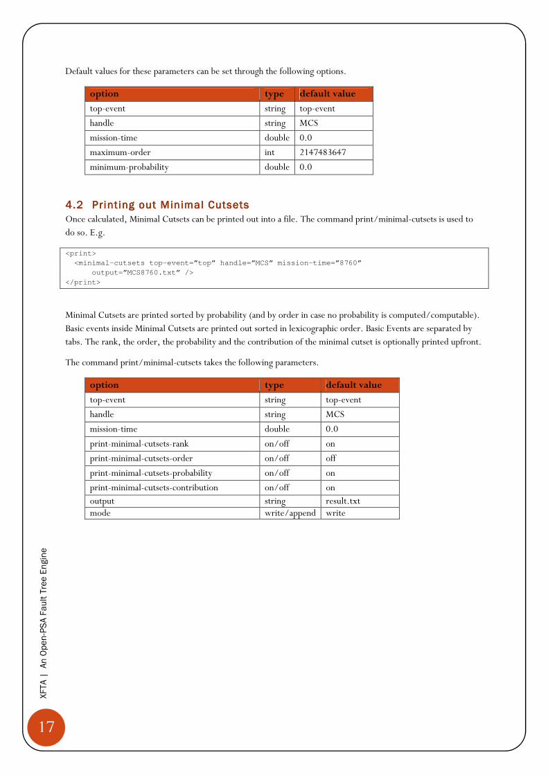
Default values for these parameters can be set through the following options.
option type default value
top-event string top-event
handle string MCS
mission-time double 0.0
maximum-order int 2147483647
minimum-probability double 0.0
4.24.24.24.2 Printing Printing Printing Printing out out out out Minimal CutsetsMinimal CutsetsMinimal CutsetsMinimal Cutsets
Once calculated, Minimal Cutsets can be printed out into a file. The command print/minimal-cutsets is used to do so. E.g.
<print>
<minimal-cutsets top-event=”top” handle=”MCS” mission-time=”8760”
output=”MCS8760.txt” />
</print>
Minimal Cutsets are printed sorted by probability (and by order in case no probability is computed/computable). Basic events inside Minimal Cutsets are printed out sorted in lexicographic order. Basic Events are separated by tabs. The rank, the order, the probability and the contribution of the minimal cutset is optionally printed upfront.
The command print/minimal-cutsets takes the following parameters.
option type default value
top-event string top-event
handle string MCS
mission-time double 0.0
print-minimal-cutsets-rank on/off on
print-minimal-cutsets-order on/off off
print-minimal-cutsets-probability on/off on
print-minimal-cutsets-contribution on/off on output string result.txt mode write/append write
18
XFTA | An Open-PSA Fault Tree Engine
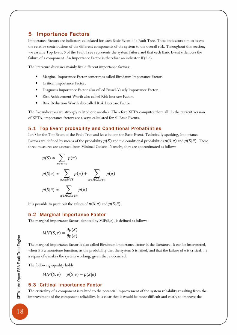
5555 Importance FactorsImportance FactorsImportance FactorsImportance Factors Importance Factors are indicators calculated for each Basic Event of a Fault Tree. These indicators aim to assess the relative contributions of the different components of the system to the overall risk. Throughout this section, we assume Top Event S of the Fault Tree represents the system failure and that each Basic Event e denotes the failure of a component. An Importance Factor is therefore an indicator IF(S,e).
The literature discusses mainly five different importance factors:
• Marginal Importance Factor sometimes called Birnbaum Importance Factor.
• Critical Importance Factor.
• Diagnosis Importance Factor also called Fussel-Vesely Importance Factor.
• Risk Achievement Worth also called Risk Increase Factor.
• Risk Reduction Worth also called Risk Decrease Factor.
The five indicators are strongly related one another. Therefore XFTA computes them all. In the current version of XFTA, importance factors are always calculated for all Basic Events.
5.15.15.15.1 Top Event probabil ity and Conditional Probabil it iesTop Event probabil ity and Conditional Probabil it iesTop Event probabil ity and Conditional Probabil it iesTop Event probabil ity and Conditional Probabil it ies
Let S be the Top Event of the Fault Tree and let e be one the Basic Event. Technically speaking, Importance
Factors are defined by means of the probability ��� and the conditional probabilities ��|�� and ��|�̅�. These three measures are assessed from Minimal Cutsets. Namely, they are approximated as follows.
��� ≈ � ����∈ !"
��|�� ≈ � ���#.�∈ !"
+ � ����∈ !",#∉�
��|�̅� ≈ � ����∈ !",#∉�
It is possible to print out the values of ��|�� and ��|�̅�. 5.25.25.25.2 Marginal Importance FactorMarginal Importance FactorMarginal Importance FactorMarginal Importance Factor
The marginal importance factor, denoted by MIF(S,e), is defined as follows.
&'(�, �� = )���)��� The marginal importance factor is also called Birnbaum importance factor in the literature. It can be interpreted, when S is a monotone function, as the probability that the system S is failed, and that the failure of e is critical, i.e. a repair of e makes the system working, given that e occurred.
The following equality holds.
&'(�, �� = ��|�� − ��|�̅� 5.35.35.35.3 Crit ical Importance FactorCrit ical Importance FactorCrit ical Importance FactorCrit ical Importance Factor
The criticality of a component is related to the potential improvement of the system reliability resulting from the improvement of the component reliability. It is clear that it would be more difficult and costly to improve the
19
XFTA | An Open-PSA Fault Tree Engine
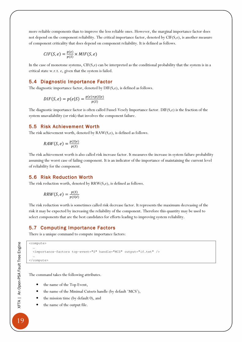
more reliable components than to improve the less reliable ones. However, the marginal importance factor does not depend on the component reliability. The critical importance factor, denoted by CIF(S,e), is another measure of component criticality that does depend on component reliability. It is defined as follows.
*'(�, �� = +#�+"� ×&'(�, ��
In the case of monotone systems, CIF(S,e) can be interpreted as the conditional probability that the system is in a critical state w.r.t. e, given that the system is failed.
5.45.45.45.4 Diagnostic Importance FactorDiagnostic Importance FactorDiagnostic Importance FactorDiagnostic Importance Factor
The diagnostic importance factor, denoted by DIF(S,e), is defined as follows.
-'(�, �� = ��|�� = +#�×+"|#�+"�
The diagnostic importance factor is often called Fussel-Vesely Importance factor. DIF(S,e) is the fraction of the system unavailability (or risk) that involves the component failure.
5.55.55.55.5 Risk Achievement WorthRisk Achievement WorthRisk Achievement WorthRisk Achievement Worth
The risk achievement worth, denoted by RAW(S,e), is defined as follows.
./0�, �� = +"|#�+"�
The risk achievement worth is also called risk increase factor. It measures the increase in system failure probability assuming the worst case of failing component. It is an indicator of the importance of maintaining the current level of reliability for the component.
5.65.65.65.6 Risk ReductioRisk ReductioRisk ReductioRisk Reduction Worthn Worthn Worthn Worth
The risk reduction worth, denoted by RRW(S,e), is defined as follows.
..0�, �� = +"�+"|#̅�
The risk reduction worth is sometimes called risk decrease factor. It represents the maximum decreasing of the risk it may be expected by increasing the reliability of the component. Therefore this quantity may be used to select components that are the best candidates for efforts leading to improving system reliability.
5.75.75.75.7 ComputComputComputComput ing ing ing ing Importance FactorsImportance FactorsImportance FactorsImportance Factors
There is a unique command to compute importance factors:
<compute>
…
<importance-factors top-event="S" handle="MCS" output="if.txt" />
…
</compute>
The command takes the following attributes.
• the name of the Top Event,
• the name of the Minimal Cutsets handle (by default ‘MCS’),
• the mission time (by default 0), and
• the name of the output file.
20
XFTA | An Open-PSA Fault Tree Engine
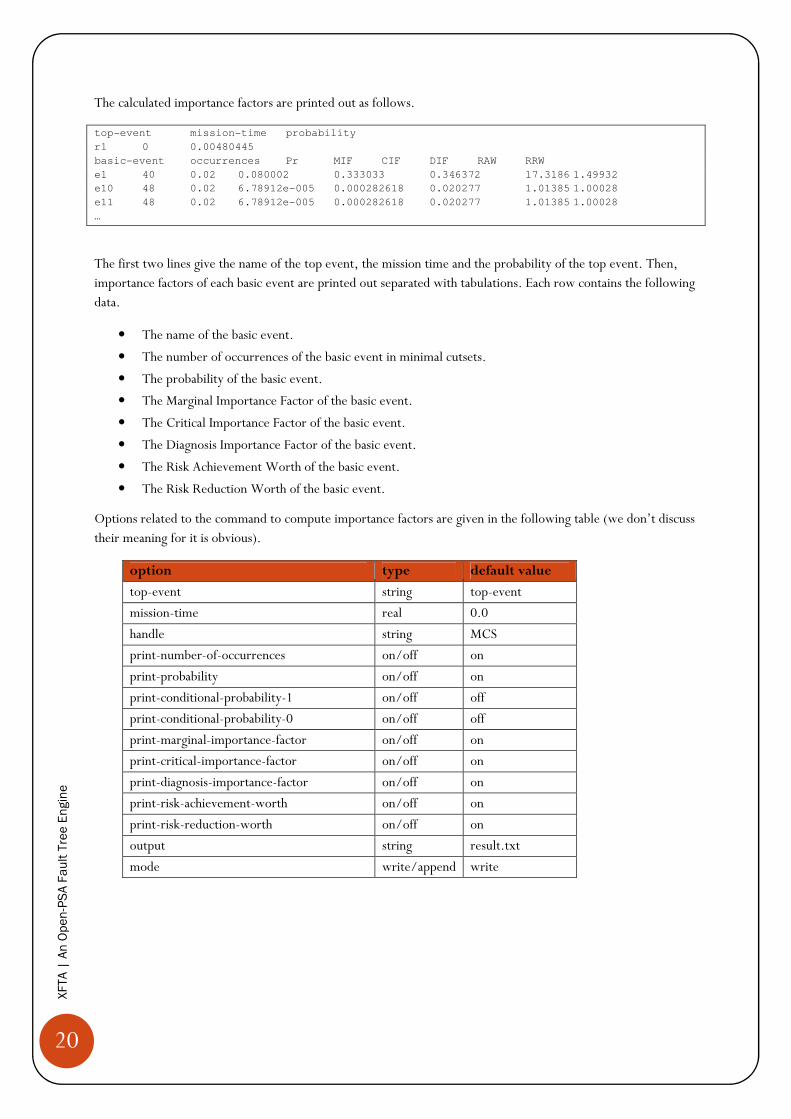
The calculated importance factors are printed out as follows.
top-event mission-time probability
r1 0 0.00480445
basic-event occurrences Pr MIF CIF DIF RAW RRW
e1 40 0.02 0.080002 0.333033 0.346372 17.3186 1.49932
e10 48 0.02 6.78912e-005 0.000282618 0.020277 1.01385 1.00028
e11 48 0.02 6.78912e-005 0.000282618 0.020277 1.01385 1.00028
…
The first two lines give the name of the top event, the mission time and the probability of the top event. Then, importance factors of each basic event are printed out separated with tabulations. Each row contains the following data.
• The name of the basic event.
• The number of occurrences of the basic event in minimal cutsets.
• The probability of the basic event.
• The Marginal Importance Factor of the basic event.
• The Critical Importance Factor of the basic event.
• The Diagnosis Importance Factor of the basic event.
• The Risk Achievement Worth of the basic event.
• The Risk Reduction Worth of the basic event.
Options related to the command to compute importance factors are given in the following table (we don’t discuss their meaning for it is obvious).
option type default value
top-event string top-event
mission-time real 0.0
handle string MCS
print-number-of-occurrences on/off on
print-probability on/off on
print-conditional-probability-1 on/off off
print-conditional-probability-0 on/off off
print-marginal-importance-factor on/off on
print-critical-importance-factor on/off on
print-diagnosis-importance-factor on/off on
print-risk-achievement-worth on/off on
print-risk-reduction-worth on/off on
output string result.txt
mode write/append write
21
XFTA | An Open-PSA Fault Tree Engine
6666 Sensitivity AnalysesSensitivity AnalysesSensitivity AnalysesSensitivity Analyses
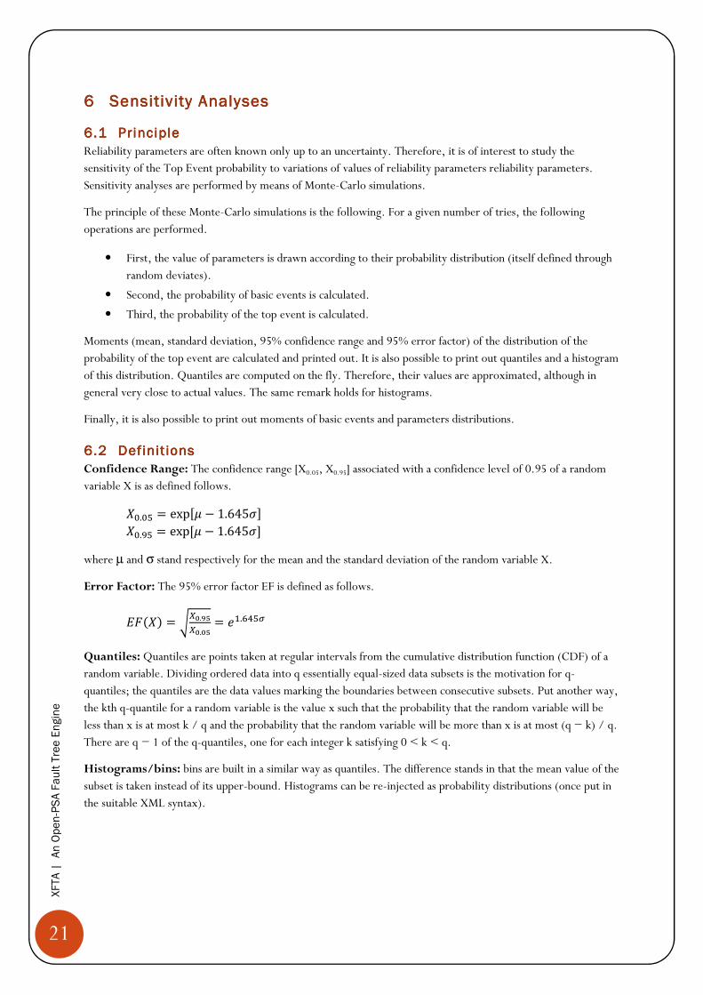
6.16.16.16.1 PrinciplePrinciplePrinciplePrinciple
Reliability parameters are often known only up to an uncertainty. Therefore, it is of interest to study the sensitivity of the Top Event probability to variations of values of reliability parameters reliability parameters. Sensitivity analyses are performed by means of Monte-Carlo simulations.
The principle of these Monte-Carlo simulations is the following. For a given number of tries, the following operations are performed.
• First, the value of parameters is drawn according to their probability distribution (itself defined through random deviates).
• Second, the probability of basic events is calculated.
• Third, the probability of the top event is calculated.
Moments (mean, standard deviation, 95% confidence range and 95% error factor) of the distribution of the probability of the top event are calculated and printed out. It is also possible to print out quantiles and a histogram of this distribution. Quantiles are computed on the fly. Therefore, their values are approximated, although in general very close to actual values. The same remark holds for histograms.
Finally, it is also possible to print out moments of basic events and parameters distributions.
6.26.26.26.2 Definit ionsDefinit ionsDefinit ionsDefinit ions
Confidence Range: The confidence range [X0.05, X0.95] associated with a confidence level of 0.95 of a random variable X is as defined follows.
12.23 = exp45 − 1.6459: 12.;3 = exp45 − 1.6459: where µ and σ stand respectively for the mean and the standard deviation of the random variable X.
Error Factor: The 95% error factor EF is defined as follows.
=(1� = >[email protected]?@.@B = �C.DE3F
Quantiles: Quantiles are points taken at regular intervals from the cumulative distribution function (CDF) of a random variable. Dividing ordered data into q essentially equal-sized data subsets is the motivation for q-quantiles; the quantiles are the data values marking the boundaries between consecutive subsets. Put another way, the kth q-quantile for a random variable is the value x such that the probability that the random variable will be less than x is at most k / q and the probability that the random variable will be more than x is at most (q − k) / q. There are q − 1 of the q-quantiles, one for each integer k satisfying 0 < k < q.
Histograms/bins: bins are built in a similar way as quantiles. The difference stands in that the mean value of the subset is taken instead of its upper-bound. Histograms can be re-injected as probability distributions (once put in the suitable XML syntax).
22
XFTA | An Open-PSA Fault Tree Engine
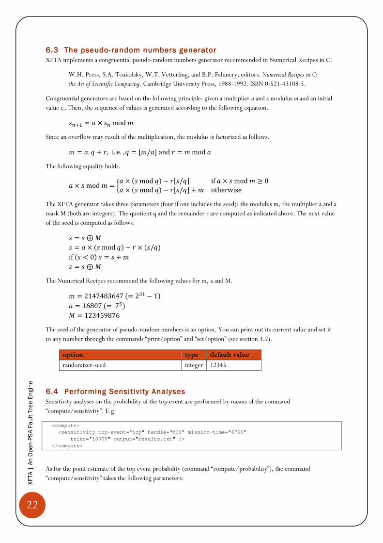
6.36.36.36.3 The pseudoThe pseudoThe pseudoThe pseudo---- random numbers generatorrandom numbers generatorrandom numbers generatorrandom numbers generator
XFTA implements a congruential pseudo-random numbers generator recommended in Numerical Recipes in C:
W.H. Press, S.A. Teukolsky, W.T. Vetterling, and B.P. Falnnery, editors. Numerical Recipes in C:
the Art of Scientific Computing. Cambridge University Press, 1988-1992. ISBN 0-521-43108-5.
Congruential generators are based on the following principle: given a multiplier a and a modulus m and an initial value s0. Then, the sequence of values is generated according to the following equation.
GHIC = J × GHmodM
Since an overflow may result of the multiplication, the modulus is factorized as follows.
M = J. N + O, i. e. , N = PM/JRandO = MmodJ
The following equality holds.
J × GmodM = SJ × GmodN� − OPG/NR ifJ × GmodM ≥ 0J × GmodN� − OPG/NR + M otherwise
The XFTA generator takes three parameters (four if one includes the seed): the modulus m, the multiplier a and a mask M (both are integers). The quotient q and the remainder r are computed as indicated above. The next value of the seed is computed as follows.
G = G ⊕&
G = J × GmodN� − O × G/N� ifG < 0�G = G + M
G = G ⊕&
The Numerical Recipes recommend the following values for m, a and M.
M = 2147483647= 2aC − 1� J = 16807= 73� & = 123459876
The seed of the generator of pseudo-random numbers is an option. You can print out its current value and set it to any number through the commands “print/option” and “set/option” (see section 3.2).
option type default value
randomizer-seed integer 12345
6.46.46.46.4 PerformPerformPerformPerforminginginging Sensit ivity AnalysesSensit ivity AnalysesSensit ivity AnalysesSensit ivity Analyses
Sensitivity analyses on the probability of the top event are performed by means of the command “compute/sensitivity”. E.g.
<compute>
<sensitivity top-event="top" handle="MCS" mission-time="8760"
tries="10000" output="results.txt" />
</compute>
As for the point estimate of the top event probability (command “compute/probability”), the command “compute/sensitivity” takes the following parameters:
23
XFTA | An Open-PSA Fault Tree Engine
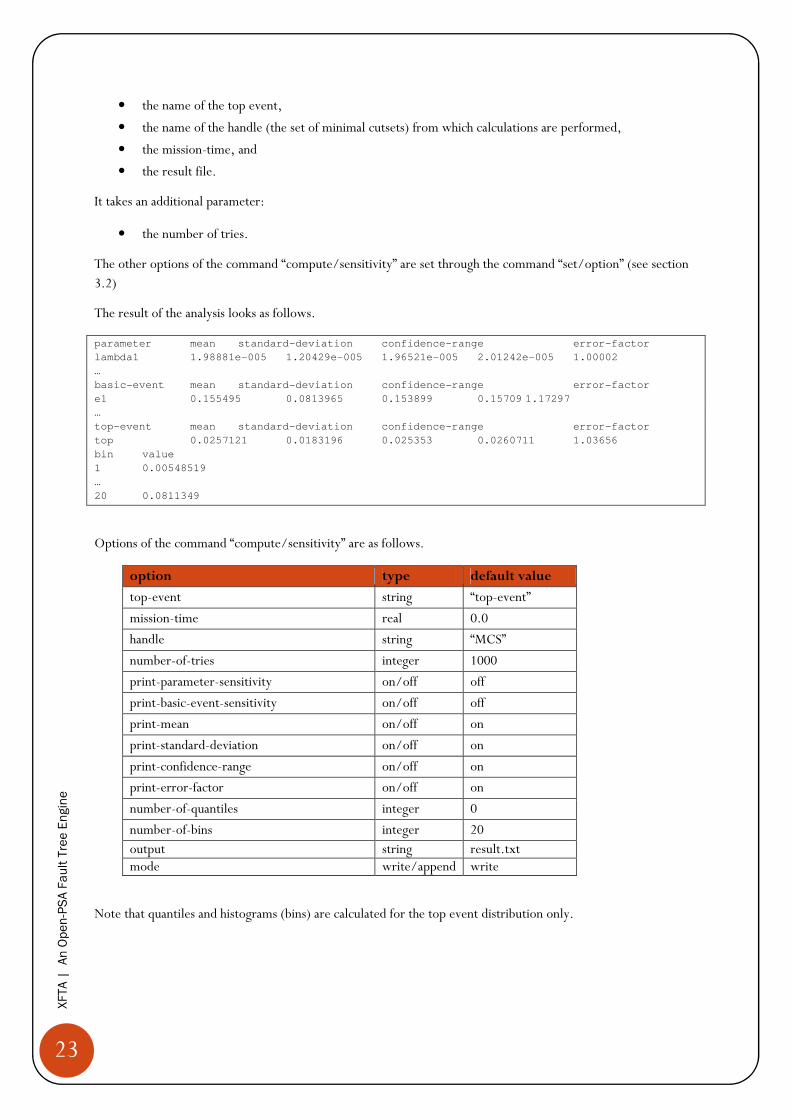
• the name of the top event,
• the name of the handle (the set of minimal cutsets) from which calculations are performed,
• the mission-time, and
• the result file.
It takes an additional parameter:
• the number of tries.
The other options of the command “compute/sensitivity” are set through the command “set/option” (see section 3.2)
The result of the analysis looks as follows.
parameter mean standard-deviation confidence-range error-factor
lambda1 1.98881e-005 1.20429e-005 1.96521e-005 2.01242e-005 1.00002
…
basic-event mean standard-deviation confidence-range error-factor
e1 0.155495 0.0813965 0.153899 0.15709 1.17297
…
top-event mean standard-deviation confidence-range error-factor
top 0.0257121 0.0183196 0.025353 0.0260711 1.03656
bin value
1 0.00548519
…
20 0.0811349
Options of the command “compute/sensitivity” are as follows.
option type default value
top-event string “top-event”
mission-time real 0.0
handle string “MCS”
number-of-tries integer 1000
print-parameter-sensitivity on/off off
print-basic-event-sensitivity on/off off
print-mean on/off on
print-standard-deviation on/off on
print-confidence-range on/off on
print-error-factor on/off on
number-of-quantiles integer 0
number-of-bins integer 20 output string result.txt mode write/append write
Note that quantiles and histograms (bins) are calculated for the top event distribution only.

24
XFTA | An Open-PSA Fault Tree Engine
7777 Safety Integrity LevelsSafety Integrity LevelsSafety Integrity LevelsSafety Integrity Levels Safety Integrity Levels (SIL) play a central role in IEC 61508 and 61511 standards and daughters. The concept of “Development Assurance Levels” of DO178B and ARP4761 standards is very similar. Safety Integrity Level is defined as a relative level of risk-reduction provided by a safety function, or to specify a target level of risk reduction. In simple terms, SIL is a measurement of performance required for a safety related system.
IEC 61508 standard identify two modes of functioning: safety related system working in low demand modes of operation, and those working in high demand or continuous modes. These two kinds of modes are arbitrarily split according to the demand frequency (lower or higher than once per year). The calculation of the average value (PFDavg) of the so-called Probability of Failure on Demand (PFD) is required for those in the first category. The calculation of the so-called Probability of Failure per Hour (PFH) is required for those in the second category.
The mode of operation should actually be determined by comparing demand and proof test frequencies: when the demand frequency is low compared to the test frequency, a failure occurring during the test interval is likely to be detected and repaired before the occurrence of a demand. Therefore the safety related system behaves almost independently from the protected installation. An accident happens if the safety related system is unable to respond (i.e. unavailable) when a demand occurs. The concept of PFD is therefore identical to the traditional concept of unavailability (which is computed by XFTA through the command compute/probability). As the frequency of demand increases (compared to the frequency of tests), the probability that the failure of the safety related system is detected and repaired decreases. It even reaches 0 in genuine continuous mode. In this case, the safety related system and the protected installation become tightly linked. If the safety related system is the only protection system of the operation process, an accident is likely to happen as soon as the former experiences its first failure (i.e. is unreliable). The concept of PFH is therefore strongly connected to the traditional concept of unreliability. The command compute/failure-intensity, introduced in this section is dedicated to this type of calculations.
In both case, it is mandatory to observe the evolution of the value of these indicators throughout a sufficiently large period of time: test intervals of each (periodically tested) components strongly influence the value of the indicator and there is nothing as an asymptotic value (at least if components are assumed to be almost as good as new after their maintenance). XFTA provides commands to evaluate the availability or the reliability of a system throughout a period of time. With Fault Trees however, the reliability can be only approximated.
This section describes the mathematical foundations as well as the XFTA commands to perform these calculations.
7.17.17.17.1 Mathematical FoundationsMathematical FoundationsMathematical FoundationsMathematical Foundations
Let S denote the system under study. Let T denote the date of the first failure of S. T is a random variable. It is called the lifetime of S. We assume that components of S were as good as new at time 0 and that they are as good as new after a repair.
Reliability RS(t) and unreliability FS(t): the reliability of S at t is the probability that S experiences no failure
during time interval [0,t], given it was working at 0. Formally,
{ }TttRdef
S <= Pr)(
The unreliability, or cumulative distribution function FS(t), is just the complement to 1 of the reliability.
{ } )(1Pr)( tRTttF S
def
S −=≥=

25
XFTA | An Open-PSA Fault Tree Engine
Failure density fS(t): The failure density refers to the probability density function of T. It is the derivative of FS(f):
dt
tFdtf S
def
S
)()( =
For sufficiently small δt’s, fS(t).δt expresses the probability that the system fails between t and t+δt, given it was
working at time 0.
Failure rate rS(t): the failure rate or hazard rate is the probability the system fails for the first time per unit of time
at age t. Formally,
{ }dt
Cdttandtbetweenfailssystemthetr dt
def
S
/Prlim)( 0
+= →
where C denotes the event “the system experienced no failure during the time interval [0,t]”. It is easy to derive
the following property from the definitions.
[ ]∫−=t
SS duurtR0
)(exp)(
Availability AS(t) and unavailability QS(t): the availability of S at t is the probability that S is working at t, given it
was working at 0.
{ }tatworkingisStAdef
S Pr)( =
The unavailability is just the complement to 1 of the availability.
)(1)( tAtQ S
def
S −=
Conditional Failure Intensity λS(t): the conditional failure intensity refers to the probability that the system fails
per unit time at time t, given it was working at time 0 and it is working at time t. Formally,
{ }dt
Ddttandtbetweenfailssystemthet dt
def
S
/Prlim)( 0
+= →λ
where D denotes the event “the system S was working at time 0 and is working at time t”. λS(t) is an indicator of
how the system is likely to fail.
Unconditional Failure Intensity wS(t): the unconditional failure intensity refers to the probability that the system
fails per unit of time at time t, given it was working at time 0. Formally,
{ }dt
Edttandtbetweenfailssystemthetw dt
def
S
/Prlim)( 0
+= →
where E denotes the event “the system was working at time 0”.
The following property holds.
)(
)()(
tA
twt
S
SS =λ
wS(t) can be calculated by means of the following property.
26
XFTA | An Open-PSA Fault Tree Engine
∑∈
=Sc
ccSS twtMIFtw )().()( ,
Where MIFS,c stands for the Marginal Importance Factor (as defined section 5) and c varies over basic events. The
above equations provide an actual mean to assess the conditional failure intensity from a fault tree model.
We can now define the average conditional failure intensity as follows.
∫×=T
SavgS dtt
Tt
0
)(1
)( λλ
7.27.27.27.2 Definit ion of Safety integrity LevelsDefinit ion of Safety integrity LevelsDefinit ion of Safety integrity LevelsDefinit ion of Safety integrity Levels
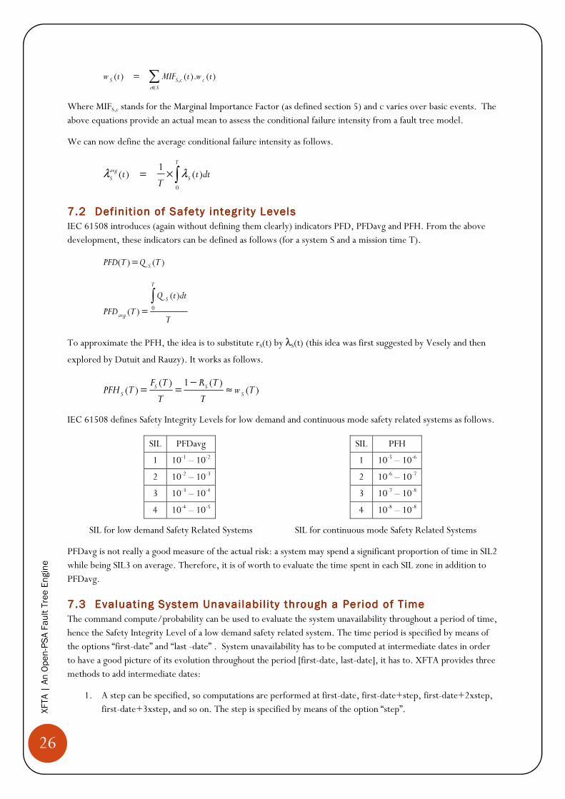
IEC 61508 introduces (again without defining them clearly) indicators PFD, PFDavg and PFH. From the above
development, these indicators can be defined as follows (for a system S and a mission time T).
)()( TQTPFD S=
T
dttQ
TPFD
T
S
avg
∫= 0
)(
)(
To approximate the PFH, the idea is to substitute rS(t) by λS(t) (this idea was first suggested by Vesely and then
explored by Dutuit and Rauzy). It works as follows.
)()(1)(
)( TwT
TR
T
TFTPFH S
SSS ≈
−==
IEC 61508 defines Safety Integrity Levels for low demand and continuous mode safety related systems as follows.
SIL PFDavg SIL PFH
1 10-1 – 10-2 1 10-5 – 10-6
2 10-2 – 10-3 2 10-6 – 10-7
3 10-3 – 10-4 3 10-7 – 10-8
4 10-4 – 10-5 4 10-8 – 10-8
SIL for low demand Safety Related Systems SIL for continuous mode Safety Related Systems
PFDavg is not really a good measure of the actual risk: a system may spend a significant proportion of time in SIL2
while being SIL3 on average. Therefore, it is of worth to evaluate the time spent in each SIL zone in addition to
PFDavg.
7.37.37.37.3 Evaluating Evaluating Evaluating Evaluating System System System System Unavailabil ity through a Period of TimeUnavailabil ity through a Period of TimeUnavailabil ity through a Period of TimeUnavailabil ity through a Period of Time
The command compute/probability can be used to evaluate the system unavailability throughout a period of time,
hence the Safety Integrity Level of a low demand safety related system. The time period is specified by means of the options “first-date” and “last -date” . System unavailability has to be computed at intermediate dates in order
to have a good picture of its evolution throughout the period [first-date, last-date], it has to. XFTA provides three
methods to add intermediate dates:
1. A step can be specified, so computations are performed at first-date, first-date+step, first-date+2xstep, first-date+3xstep, and so on. The step is specified by means of the option “step”.
27
XFTA | An Open-PSA Fault Tree Engine
2. Singular points can be automatically calculated from probability distributions of basic events. Periodic
test distributions create such singular points at the beginning and the end of test period. To add singular
points, the option “add-singular-points” must be turned on. 3. The curve can be automatically smoothed. Smoothing the curve is done by adding an intermediate date
tm=(t1+t2)/2 in the middle of each pair (t1,t2) of successive dates. Then, the calculated value Prc = Pr(tm)
is compare to the estimated value Pre =(Pr(t1)+Pr(t2))/2. If the relative difference |Prc-Pre|/Prc is
greater than the smoothing ratio, then the pairs (t1,tm) and (tm,t2) are considered in turn. To smooth the
curve, the option “smooth-curve” must be turned on. The smoothing ration is specified by the option “smoothing-ratio”.
These three methods can be used separately or together. Once the curve of unavailability calculated, three
different results can be printed out:
• the curve itself (by turning on the option “print-unavailability”),
• the curve of the average value of the unavailability from the first date to the current date (by turning on
the option “print-average-unavailability”), and
• the sojourn times spent in each safety integrity level. The system is considered here in low demand mode.
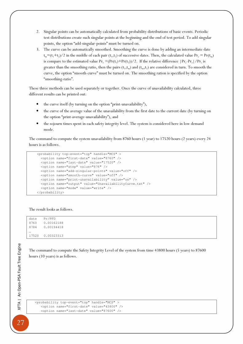
The command to compute the system unavailability from 8760 hours (1 year) to 17520 hours (2 years) every 24
hours is as follows.
<probability top-event="top" handle="MCS" >
<option name="first-date" value="8760" />
<option name="last-date" value="17520" />
<option name="step" value="876" />
<option name="add-singular-points" value="off" />
<option name="smooth-curve" value="off" />
<option name=”print-unavailability” value=”on” />
<option name="output" value="UnavailabilityCurve.txt" />
<option name="mode" value="write" />
</probability>
The result looks as follows.
date Pr/PFD
8760 0.00162188
8784 0.00194418
…
17520 0.00323313
The command to compute the Safety Integrity Level of the system from time 43800 hours (5 years) to 87600
hours (10 years) is as follows.
<probability top-event="top" handle="MCS" >
<option name="first-date" value="43800" />
<option name="last-date" value="87600" />
28
XFTA | An Open-PSA Fault Tree Engine
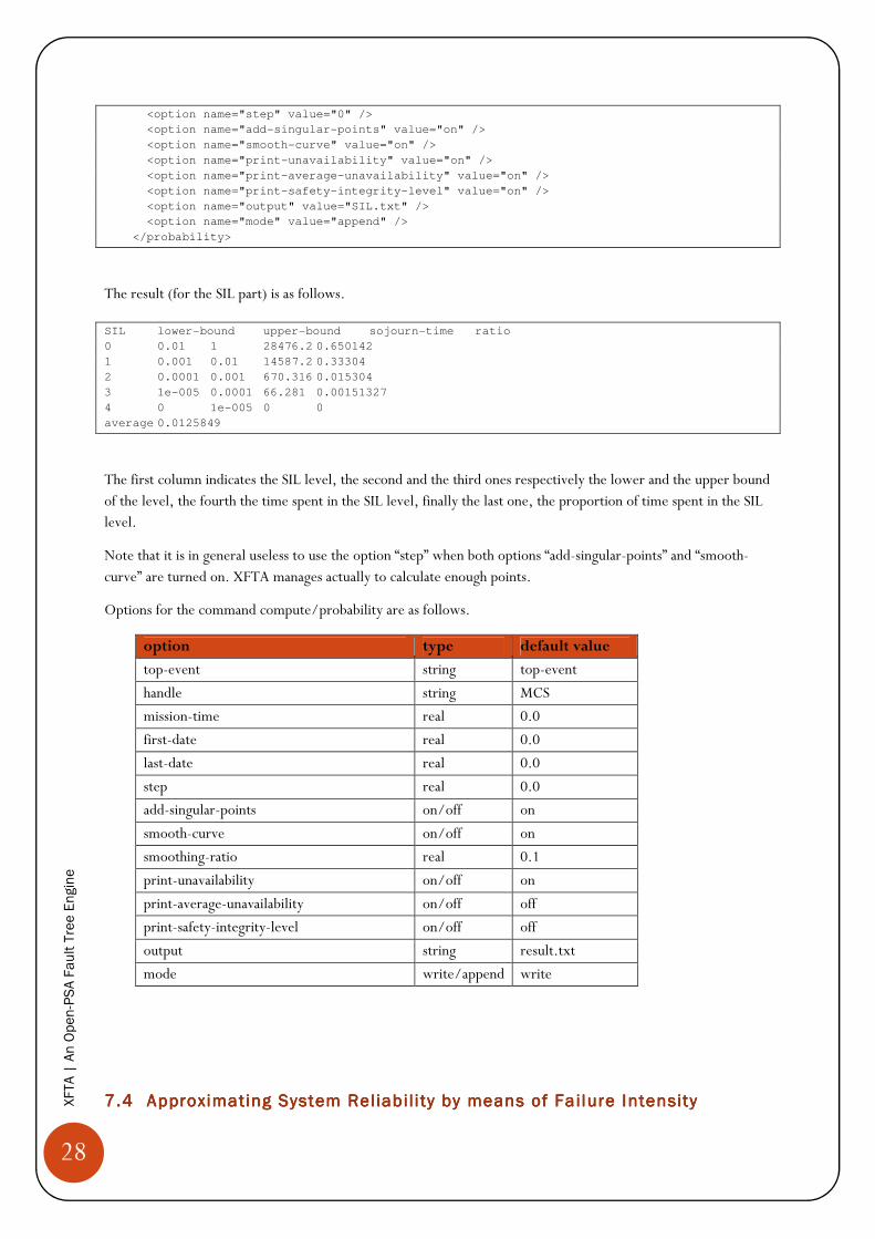
<option name="step" value="0" />
<option name="add-singular-points" value="on" />
<option name="smooth-curve" value="on" />
<option name="print-unavailability" value="on" />
<option name="print-average-unavailability" value="on" />
<option name="print-safety-integrity-level" value="on" />
<option name="output" value="SIL.txt" />
<option name="mode" value="append" />
</probability>
The result (for the SIL part) is as follows.
SIL lower-bound upper-bound sojourn-time ratio
0 0.01 1 28476.2 0.650142
1 0.001 0.01 14587.2 0.33304
2 0.0001 0.001 670.316 0.015304
3 1e-005 0.0001 66.281 0.00151327
4 0 1e-005 0 0
average 0.0125849
The first column indicates the SIL level, the second and the third ones respectively the lower and the upper bound
of the level, the fourth the time spent in the SIL level, finally the last one, the proportion of time spent in the SIL level.
Note that it is in general useless to use the option “step” when both options “add-singular-points” and “smooth-
curve” are turned on. XFTA manages actually to calculate enough points.
Options for the command compute/probability are as follows.
option type default value
top-event string top-event
handle string MCS
mission-time real 0.0
first-date real 0.0
last-date real 0.0
step real 0.0
add-singular-points on/off on
smooth-curve on/off on
smoothing-ratio real 0.1
print-unavailability on/off on
print-average-unavailability on/off off
print-safety-integrity-level on/off off
output string result.txt
mode write/append write
7.47.47.47.4 Approximating System Reliabil i ty Approximating System Reliabil i ty Approximating System Reliabil i ty Approximating System Reliabil i ty by means ofby means ofby means ofby means of Failure IntensityFailure IntensityFailure IntensityFailure Intensity
29
XFTA | An Open-PSA Fault Tree Engine
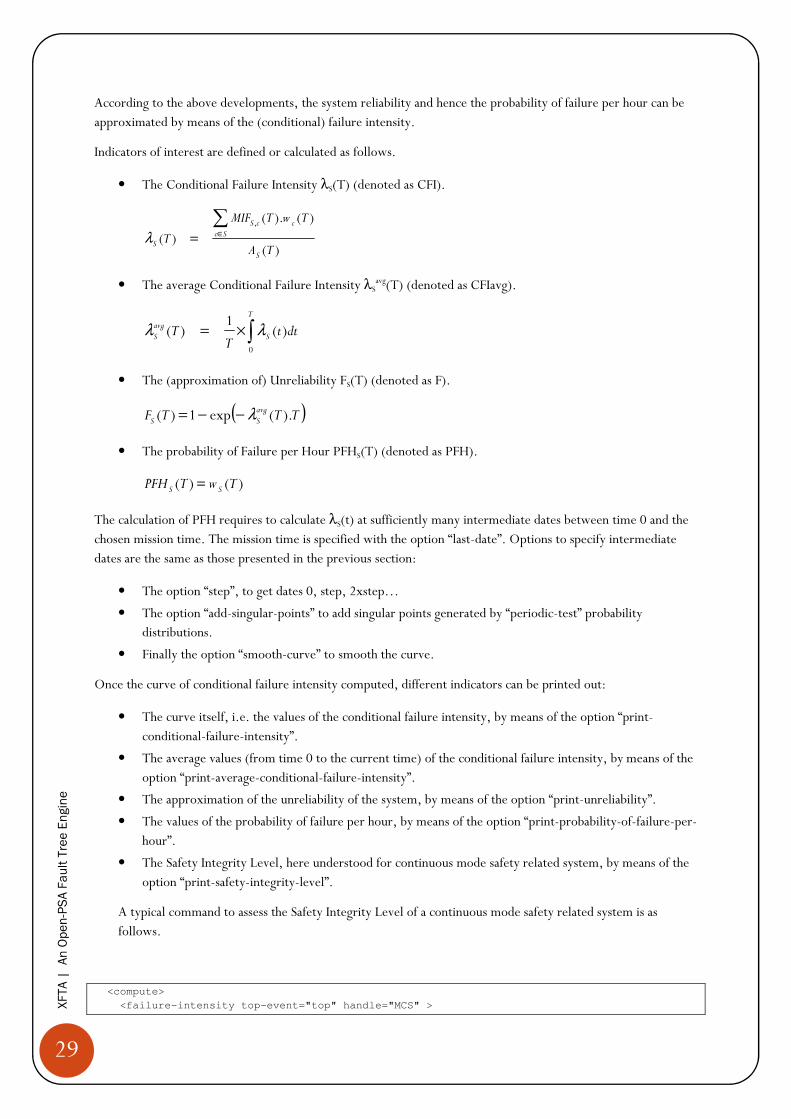
According to the above developments, the system reliability and hence the probability of failure per hour can be
approximated by means of the (conditional) failure intensity.
Indicators of interest are defined or calculated as follows.
• The Conditional Failure Intensity λS(T) (denoted as CFI).
)(
)().(
)(,
TA
TwTMIF
TS
ScccS
S
∑∈=λ
• The average Conditional Failure Intensity λSavg(T) (denoted as CFIavg).
∫×=T
SavgS dtt
TT
0
)(1
)( λλ
• The (approximation of) Unreliability FS(T) (denoted as F).
( )TTTF avgSS ).(exp1)( λ−−=
• The probability of Failure per Hour PFHS(T) (denoted as PFH).
)()( TwTPFH SS =
The calculation of PFH requires to calculate λS(t) at sufficiently many intermediate dates between time 0 and the
chosen mission time. The mission time is specified with the option “last-date”. Options to specify intermediate
dates are the same as those presented in the previous section:
• The option “step”, to get dates 0, step, 2xstep…
• The option “add-singular-points” to add singular points generated by “periodic-test” probability distributions.
• Finally the option “smooth-curve” to smooth the curve.
Once the curve of conditional failure intensity computed, different indicators can be printed out:
• The curve itself, i.e. the values of the conditional failure intensity, by means of the option “print-
conditional-failure-intensity”.
• The average values (from time 0 to the current time) of the conditional failure intensity, by means of the
option “print-average-conditional-failure-intensity”.
• The approximation of the unreliability of the system, by means of the option “print-unreliability”.
• The values of the probability of failure per hour, by means of the option “print-probability-of-failure-per-
hour”.
• The Safety Integrity Level, here understood for continuous mode safety related system, by means of the
option “print-safety-integrity-level”.
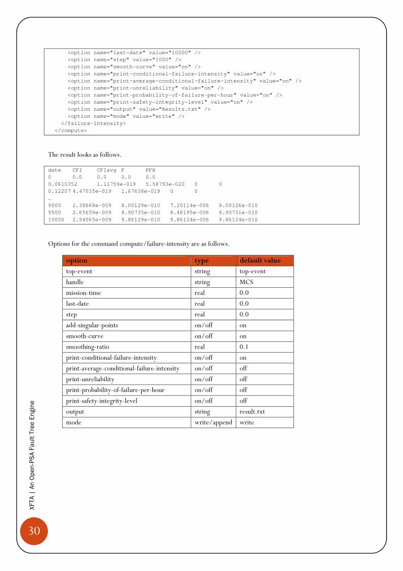
A typical command to assess the Safety Integrity Level of a continuous mode safety related system is as
follows.
<compute>
<failure-intensity top-event="top" handle="MCS" >
30
XFTA | An Open-PSA Fault Tree Engine
<option name="last-date" value="10000" />
<option name="step" value="1000" />
<option name="smooth-curve" value="on" />
<option name="print-conditional-failure-intensity" value="on" />
<option name="print-average-conditional-failure-intensity" value="on" />
<option name="print-unreliability" value="on" />
<option name="print-probability-of-failure-per-hour" value="on" />
<option name="print-safety-integrity-level" value="on" />
<option name="output" value="Results.txt" />
<option name="mode" value="write" />
</failure-intensity>
</compute>
The result looks as follows.
date CFI CFIavg F PFH
0 0.0 0.0 0.0 0.0
0.0610352 1.11759e-019 5.58793e-020 0 0
0.12207 4.47035e-019 1.67638e-019 0 0
…
9000 2.38668e-009 8.00129e-010 7.20114e-006 8.00126e-010
9500 2.65659e-009 8.90735e-010 8.46195e-006 8.90731e-010
10000 2.94065e-009 9.86129e-010 9.86124e-006 9.86124e-010
Options for the command compute/failure-intensity are as follows.
option type default value
top-event string top-event
handle string MCS
mission-time real 0.0
last-date real 0.0
step real 0.0
add-singular-points on/off on
smooth-curve on/off on
smoothing-ratio real 0.1
print-conditional-failure-intensity on/off on
print-average-conditional-failure-intensity on/off off
print-unreliability on/off off
print-probability-of-failure-per-hour on/off off
print-safety-integrity-level on/off off
output string result.txt
mode write/append write

31
XFTA | An Open-PSA Fault Tree Engine
8888 Known BugsKnown BugsKnown BugsKnown Bugs “If debugging is the process of removing bugs, then programming must be the process of putting them in.” E.W. Dijskra.
Bug-2012-10-10-a: Simplification of formulas with constant or house-event works improperly, therefore raising
an undue syntax error. Fixed in version 1.1.