an old new notation for elementary probability theorycarrollm/probs/papers/morgan-13.pdf · an old...
TRANSCRIPT
An old new notationfor elementary probability theory
Carroll Morgan
University of New South Wales, NSW 2052 [email protected] ?
Abstract. The Eindhoven approach to quantifier notation is 40 yearsold. We extend it by adding “distribution comprehensions” systemati-cally to its repertiore; we believe the resulting notation for elementaryprobability theory is new.After a step-by-step explanation of the proposed notational innovations,with small examples, we give as our exemplary case study the probabilis-tic reasoning associated with a quantitative noninterference semanticsbased on Hidden Markov Models of computation. Although that exam-ple was the motivation for this work, we believe the proposal here willbe more generally applicable: and so we also revisit a number of popularpuzzles, to illustrate the notation’s wider utility.
Finally, we review the connection between comprehension notationsand (category-theoretic) monads, and show how the Haskell approachto monad comprehensions applies to the distribution comprehensions wehave introduced.
1 Context and motivation
Conventional notations for elementary probability theory are more descriptivethan calculational. They communicate ideas, but they are not algebraic (as arule) in the sense of helping to proceed reliably from one idea to the next one:and truly effective notations are those that we can reason with rather than simplyabout. In our recent work on security, the conventional notations for probabilitybecame so burdensome that we felt that it was worth investigating alternative,more systematic notations for their own sake.
The Eindhoven notation was designed in the 1970’s to control complexity inreasoning about programs and their associated logics: the forty years since thenhave shown how effective it is. But as far as we know it has not been used forprobability. We have done so by working “backwards,” from an application incomputer security (Sec. 9.2), with the Eindhoven style as a target (Sec. 2). Thatis the opposite, incidentally, of reconstructing elementary probability “forwards”from first principles — also a worthwhile goal, but a different one.
We judge our proposal’s success by whether it simplifies reasoning aboutintricate probabilistic structures in computer science and elsewhere. For that
? This article extends an earlier publication XXX. We are grateful for the support ofthe Dutch NWO (Grant 040.11.303) and the Australian ARC (Grant DP1092464).

2 Carroll Morgan
we give a small case study, based on noninterference-security semantics, both inthe novel notation and in the conventional notation; and we compare them witheach other (Sec. 9). We have also used the new notation more extensively [18].
Although the notation was developed retroactively, the account we give hereis forwards, that is from the basics towards more advanced constructions. Alongthe way we use a number of popular puzzles as more general examples.
2 The Eindhoven quantifier notation, and our extension
In the 1970’s, researchers at THE in Eindhoven led by E.W. Dijkstra proposeda uniform notation for quantifications in first-order logic, elementary set theoryand related areas [5]. By (Qx:T | rng · exp) 1 they meant that quantifier Q bindsvariable x of type T within textual scope (· · · ), that x is constrained to satisfyformula rng, that expression exp is evaluated for each such x and that thosevalues then are combined via an associative and commutative operator related toquantifier Q. These examples make the uniformity evident:
(∀x:T | rng · exp) means for all x in T satisfying rng we have exp,
(∃x:T | rng · exp) means for some x in T satisfying rng we have exp,
(Σx:T | rng · exp) means the sum of all exp for x in T satisfying rng ,
{x:T | rng · exp} means the set of all exp for x in T satisfying rng .
A general shorthand applying to them all is that an omitted range |rng defaultsto |true, and an omitted ·exp defaults to the bound variable ·x itself.
These (once) novel notations are not very different from the conventionalones: they contain the same ingredients because they must. Mainly they are areordering, an imposition of consistency, and finally a making explicit of what isoften implicit: bound variables, and their scope. Instead of writing {n∈N | n>0}for the positive natural numbers we write {n:N | n>0}, omitting the “·n” via theshorthand above; the only difference is the explicit declaration of n via a colon(as in a programming language) rather than via n∈N which, properly speaking, isa formula (with both n and N free) and doesn’t declare anything. And instead of{n2 | n∈N} for the square numbers, we write {n:N · n2}, keeping the declarationin first position (always) and avoiding ambiguous use of the vertical bar.
In program semantics one can find general structures such as
sets of distributions for probability and nondeterminism [24, 17],
distributions of distributions,for probabilistic noninterference security [18, 19], and even
sets of distributions of distributions to combine the two [20].
1 The original Eindhoven style uses colons as separators; the syntax here with | and
· is more in the Z style [11], and is one of many subsequent notational variationsbased on their innovation.

An old new notation for elementary probability theory 3
All of these are impeded by the conventional use of “Pr” to refer to probabilitywith respect to some unnamed distribution “of interest” at the time: we need torefer to the whole distribution itself.
And when we turn to particular instances, the semantics of individual pro-grams, we need to build functions corresponding to specific program compo-nents. The conventional “random variables” are inconvenient for this, since wemust invent a name for every single one: we would rather use the expressions andvariables occurring in the programs themselves. In the small –but nontrivial– ex-ample of information flow (Sec. 9), borrowed from our probabilistic security work[18–20], we compare the novel notation (Sec. 9.2) to the conventional (Sec. 9.3)in those respects.
Our essential extension of the Eindhoven quantifiers was to postulate a “dis-tribution comprehension” notation {{s: δ | rng · exp}}, intending it to mean “forall elements s in the distribution δ, conditioned by rng , make a new distributionbased on evaluating exp.” Thus we refer to a distribution itself (the whole com-prehension), and we access random variables as expressions (the exp within).From there we worked backwards, towards primitives, to arrange that indeedthe comprehension would have that meaning.
This report presents our results, but working forwards and giving simpleexamples as we go. Only at Def. 13 do we finally recover our conceptual startingpoint, a definition of the comprehension that agrees with the guesswork justabove (Sec. 8.5).
3 Discrete distributions as enumerations
We begin with distributions written out explicitly: this is by analogy with theenumerations of sets which list their elements. The notation f.x for applicationof function f to argument x is used from here on, except for type constructorswhere a distinct font allows us to reduce clutter by omitting the dot.
3.1 Finite discrete distributions as a type
A finite discrete distribution δ on a set S is a function assigning to each elements in S a (non-negative) probability δ.s, where the sum of all such probabilitieson S is one. The fair distribution on coin-flip outcomes {H,T} takes both H,Tto 1/2; the distribution on die-roll outcomes {1··6} for a fair die gives 1/6 foreach integer n with 1≤n≤6. In general we have
Definition 1. The constructor D for finite discrete distributionsThe set DS of discrete distributions over a finite set S is the functions from
S into [0, 1] that sum to one, that is {δ:S→[0, 1] | (Σs:S · δ.s) = 1}. The set Sis called the basis (type) of δ. 2
In Def. 1 the omitted |rng of∑
is |true, and the omitted ·exp of {· · · } is ·δ.One reason for using distinct symbols | and · is that in the default cases thosesymbols can be omitted as well, with no risk of ambiguity.

4 Carroll Morgan
3.2 The support of a distribution
The support of a distribution is that subset of its basis to each of whose ele-ments it assigns nonzero probability; it is in an informal sense the “relevant” or“interesting” elements in the distribution. We define
Definition 2. Support of a distribution For distribution δ:DS with basis S,the support is the subset dδe:= {s:S | δ.s 6=0} of S. 2
The “ceiling” notation d·e suggests the pointwise ceiling of a distribution which,as a function (Def. 1), is the characteristic function of its support.
3.3 Specialised notation for uniform distributions
By analogy with set enumerations like {H,T}, we define uniform-distributionenumerations that assign the same probability to every element in their support:
Definition 3. Uniform-distribution enumeration The uniform distribution overan enumerated set {a, b, · · · , z} is written {{a, b, · · · , z}}. It is assumed that thevalues a, b, · · · , z are distinct and that there is at least one. 2
Thus for example the fair-coin distribution is {{H,T}} and the fair-die distributionis {{1··6}}.
As a special case of uniform distribution we have the point distribution {{a}}on some element a, assigning probability 1 to it: this is analogous to the singletonset {a} that contains only a.
3.4 General notation for distribution enumerations
For distributions that are not uniform, we attach a probability explicitly to each
element. Thus we have {{H@ 23 ,T@ 1
3 }} for the coin that is twice as likely to give
heads H as tails T, and {{1@ 29 , 2@
19 , 3@
29 , 4@
19 , 5@
29 , 6@
19 }} for the die that is twice
as likely to roll odd as even (but is uniform otherwise). In general we have
Definition 4. Distribution enumeration We write {{a@pa , b@pb , · · · , z@pz}} forthe distribution over set {a, b, · · · , z} that assigns probability pa to element aetc. For well-formedness we require that pa+pb+ · · ·+pz = 1. 2
3.5 The support of a distribution is a subset of its basis
Strictly speaking one can’t tell, just by drawing samples, whether {{H,T}} rep-resents the distribution of a fair two-sided coin, or instead represents the dis-tribution of a three-sided coin with outcomes {H,T,E} that never lands on itsedge E. Similarly we might not know whether {{6}} describes a die that has thenumeral 6 written on every face or a loaded die that always rolls 6.
Saying that δ is uniform over S means it is uniform and its support is S.
An old new notation for elementary probability theory 5
3.6 Specialised infix notations for making distributions
For distributions of support no more than two we have the special notation
Definition 5. Doubleton distribution For any elements a, b and 0≤p≤1 wewrite a p⊕ b for the distribution {{a@p, b@1−p}}. 2
Thus the fair-coin distribution {{H,T}} can be written H1/2⊕T. For the weightedsum of two distributions we have
Definition 6. Weighted sum For two numbers x, y and 0≤p≤1 we define thesum x p+y:= px+(1−p)y; more generally x, y can be elements of a vector space.
In particular, for two distributions δ, δ′:DS we define their weighted sumδ p+ δ′ by (δ p+ δ′).s := p(δ.s) + (1−p)(δ′.s) for all s in S. 2
Thus the biased die from Sec. 3.4 can be written as {{1, 3, 5}} 2/3+ {{2, 4, 6}},showing at a glance that its odds and evens are uniform on their own, but thatcollectively the odds are twice as likely as the evens.
As simple examples of algebra we have first x p⊕ y = {{x}} p+ {{y}}, and then
δ 0+ δ′ = δ′ and δ 1+ δ′ = δand dδ p+ δ′e = dδe ∪ dδ′e when 0<p<1.
3.7 Comparison with conventional notation 2
Conventionally a distribution is over a sample space S, which we have called thebasis (Def. 1). Subsets of the sample space are events, and a distribution assignsa number to every event, the probability that an observation “sampled” fromthe sample space will be an occurrence of that event. That is, a distribution isof type PS→[0, 1] from subsets of S rather than from its elements.
With our odd-biased die in Sec. 3.4 the sample space is S={1··6} and theprobability 2/3 of “rolled odd,” that is of the event {1, 3, 5}⊂S, is twice theprobability 1/3 of “rolled even,” that is of the event {2, 4, 6}⊂S.
There are “additivity” conditions placed on general distributions, amongwhich are that the probability assigned to the union of two disjoint events shouldbe the sum of the probabilities assigned to the events separately, that the prob-ability assigned to all of S should be one, and that the probability assigned tothe empty event should be zero.
When S is finite, the general approach specialises so that a discrete distri-bution δ acts on separate points, instead of on sets of them. The probability ofany event S′⊂S is then just
∑s∈S′ δ(s) from additivity.
2 When presenting examples in conventional notation, in this and later comparisonsections, we will write f(x) instead of f.x and {exp | x∈S} instead of {x:S · exp}.

6 Carroll Morgan
4 Expected values over discrete distributions
4.1 Definition of expected value as average
If the basis S of a distribution δ:DS comprises numbers or, more generally, isa vector space, then the “weighted average” of the distribution is the sum ofthe values in S multiplied by the probability that δ assigns to each, that is(Σs:S · δ.s×s). For the fair die that becomes (1+2+3+4+5+6)/6 = 31/2; forthe odd-biased die the average is 42/3.
For the fair coin {{H,T}} however we have no average, since {H,T} has noarithmetic. We must work indirectly via a function on the basis, using
Definition 7. Expected value By (Es: δ · exp) we mean the expected value offunction (λ s · exp) over distribution δ; it is
(Es: δ · exp) := (Σs: dδe · δ.s×exp) . 3
Note that exp is an expression in which bound variable s probably appears(though it need not). We call exp the constructor. 2
For example, the expected value of the square of the value rolled on a fair die is(Es: {{1··6}} · s2) = (12 + · · ·+ 62)/6 = 151/6.
For further examples, we name a particular distribution δ̂:= {{0, 1, 2}} anddescribe a notation for converting Booleans to numbers:
Definition 8. Booleans converted to numbers The function [·] takes BooleansT,F to numbers 0,1 so that [T]:= 1 and [F]:= 0. 4 2
Then we have
(Es: δ̂ · smod 2) = 1/3×0 + 1/3×1 + 1/3×0 = 1/3
and (Es: δ̂ · [s6=0]) = 1/3×0 + 1/3×1 + 1/3×1 = 2/3 ,
where in the second case we have used Def. 8 to convert the Boolean s6=0 to anumber. Now we can formulate the average proportion of heads shown by a faircoin as (Es: {{H,T}} · [s=H]) = 1/2.
4.2 The probability of a subset rather than of a single element
We can use the expected value quantifier to give the aggregate probability as-signed to a (sub)set of outcomes, provided we have a formula describing thatset. 5 When exp is Boolean, we have that (Es: δ · [exp]) is the probability as-signed by δ to the whole of the set {s: dδe | exp}. This is because the expectedvalue of the characteristic function of a set is equal to the probability of thatset as a whole. An example of this occurs just after Def. 8; another is given at4.3(e) below.
3 Here is an example of not needing to know the basis type: we simply sum over thesupport of δ, since the other summands will be zero anyway.
4 We disambiguate T for true and T for tails by context.5 Note that those aggregate probabilities do not sum to one over all subsets of the
basis, since the individual elements would be counted many times.
An old new notation for elementary probability theory 7
4.3 Abbreviation conventions
The following are five abbreviations that we use in the sequel.
(a) If several bound variables are drawn from the same distribution, we as-sume they are drawn independently from separate instances of it. Thus(Ex, y: δ · · · ·) means (Ex: δ; y: δ · · · ·) or equivalently (E(x, y): δ2 · · · ·).
(b) If in an expected-value quantification the exp is omitted, it is taken to bethe bound variable standing alone (or a tuple of them, if there are sev-eral). Thus (Es: δ) means (Es: δ · s), and more generally (Ex, y: δ) means(Ex, y: δ · (x, y)) with appropriate arithmetic induced on dδe×dδe.
(c) By analogy with summation, where for a set S we abbreviate (Σs:S) by∑S, we abbreviate (Es: δ) by Eδ. Thus E δ̂ = E{{0, 1, 2}} = (0+1+2)/3 = 1.
(d) If a set is written where a distribution is expected, we assume implicitly that
it is the uniform distribution over that set. Thus E{0, 1, 2} = E δ̂ = 1.(e) If a Boolean expression occurs where a number is expected, then we as-
sume an implicit application of the conversion function [·] from Def. 8. Thus(Es: {0, 1, 2} · s6=0) = 2/3 is the probability that a number chosen uniformlyfrom 0, 1, 2 will not be zero.
4.4 Example of expected value: dice at the fairground
Define the set D to be {1··6}, the possible outcomes of a die roll.At the fairground there is a tumbling cage with three fair dice inside, and a
grid of six squares marked by numbers from D. You place $1 on a square, andwatch the dice tumble until they stop.
If your number appears exactly once among the dice, then you get your $1back, plus $1 more; if it appears twice, you get $2 more; if it appears thrice youget $3 more. If it’s not there at all, you lose your $1.
Using our notation so far, your expected profit is written
−1 + (Es1, s2, s3:D · (∨ i · si=s) + (Σi · si=s)) , (1)
where the initial −1 accounts for the dollar you paid to play, and the free variables is the number of the square on which you placed it. The disjunction describesthe event that you get your dollar back; and the summation describes the extradollars you (might) get as well.
The D is converted to a uniform distribution by 4.3(d), then replicated threetimes by 4.3(a), independently for s{1,2,3}; and the missing conversions fromBoolean to 0,1 are supplied by 4.3(e).
Finally we abuse notation by writing si even though i is itself a (bound)variable: e.g. by (
∨i · si=s) we mean in fact s1=s ∨ s2=s ∨ s3=s. 6
6 It is an abuse because in the scope of i we are using it as if it were an argumentto some function s(·) — but the s is is already used for something else. Moreovers1, s2, s3 must themselves be names (not function applications) since we quantifyover them with E . Also we gave no type for i.

8 Carroll Morgan
While the point of this example is the way in which (1) is written, for thosetempted to play this game it’s worth pointing out that its value is approximately−.08, independent of s. That is an expected loss of about eight cents in the dollaron every play and no matter which square is chosen.
4.5 Comparison with conventional notation
Conventionally, expected values are taken over random variables that are func-tions from the sample space into a set with arithmetic, usually the reals (butmore generally a vector space). Standard usage is first to define the sample space,then to define a distribution over it, and finally to define a random variable overthe sample space and give it a name, say X. Then one writes Pr(X=x) forthe probability assigned by that distribution to the event that the (real-valued)random variable X takes some (real) value x; and E(X) is the notation for theexpected value of random variable X over the same (implicit) distribution.
In Def. 7 our random variable is (λ s · exp), and we can write it withouta name since its bound variable s is already declared. Furthermore, becausewe can give the distribution δ explicitly, we can write expressions in which thedistributions are themselves expressions. As examples, we have
(Es: {{e}} · exp) = exp[s\e] – one-point rule(Es: (δ p+ δ′) · exp) = (Es: δ · exp) p+ (Es: δ′ · exp) – using Def. 6(Es: (x p⊕ y) · exp) = exp[s\x] p+ exp[s\y] – from the two above,
where exp[s\e] is bound-variable-respecting replacement of s by e in exp.For example, if δ is the distribution of random variable X, then the conven-
tional Pr(X=x) becomes δ.x, and E(X) becomes Eδ.
5 Discrete distributions as comprehensions
5.1 Definition of distribution comprehensions
With a comprehension, a distribution is defined by properties rather than byenumeration. Just as the set comprehension {s: dδ̂e · s2} gives the set {0, 1, 4}having the property that its elements are precisely the squares of the elementsof dδ̂e = {0, 1, 2}, we would expect {{s: δ̂ · s2}} to be {{0, 1, 4}} where in this case
the uniformity of the source δ̂ has induced uniformity in the target.If however some of the target values “collide,” because exp is not injec-
tive, then their probabilities add together: thus we have {{s: δ̂ · s mod 2}} =
Although our purpose is to show how we achieve a concise presentation withprecise notation, we are at the same time arguing that “to abuse, or not to abuse”should be decided on individual merits. There are times when a bit of flexibility ishelpful: arguably the abuse here gains more in readability than it loses in informality.
A similar use is (∃i · · · ·Hi · · ·) for the weakest precondition of a loop: this fi-nesse avoided swamping a concise first-order presentation with (mostly unnecessary)higher-order logic throughout [4].

An old new notation for elementary probability theory 9
{{0@ 23 , 1@
13 }} = 0 2/3⊕ 1, where target element 0 has received 1/3 probability as
0 mod 2 and another 1/3 as 2 mod 2.
We define distribution comprehensions by giving the probability they assignto an arbitrary element; thus
Definition 9. Distribution comprehension For distribution δ and arbitraryvalue e of the type of exp we define
{{s: δ · exp}}.e := (Es: δ · [exp=e]) . 7
2
The construction is indeed a distribution on {s: dδe · exp} (Lem. 1 in App. C),and assigns to element e the probability given by δ that exp=e as s ranges overthe basis of δ. 8
Note that {{s: δ}} is therefore just δ itself.
5.2 Examples of distribution comprehensions
We have from Def. 9 that the probability {{s: δ̂ · smod 2}} assigns to 0 is
{{s: δ̂ · smod 2}}.0= (Es: δ̂ · [smod 2 = 0])= 1/3×[0=0] + 1/3×[1=0] + 1/3×[0=0]= 1/3×1 + 1/3×0 + 1/3×1= 2/3 ,
and the probability {{s: δ̂ · smod 2}} assigns to 1 is
{{s: δ̂ · smod 2}}.1= 1/3×[0=1] + 1/3×[1=1] + 1/3×[0=1]= 1/3 .
Thus we have verified that {{s: δ̂ · smod 2}} = 0 2/3⊕ 1 as stated in Sec. 5.1.
7 Compare {x:X · exp}3e defined to be (∃x:X · exp=e).8 A similar comprehension notation is used in cryptography, for example the
{s R←− S; s′R←− S′ : exp}
that in this case takes bound variables (s, s′) uniformly (R←−) from sample spaces
(S, S′) and, with them, makes a new distribution via a constructor expression (exp)containing those variables. We would write that as {{s:S; s′:S′ · exp}} with the S, S′
converted to uniform distributions by 4.3(d).

10 Carroll Morgan
5.3 Comparison with conventional notation
Conventionally one makes a target distribution from a source distribution by“lifting” some function that takes the source sample space into a target. Weexplain that here using the more general view of distributions as functions ofsubsets of the sample space (Sec. 3.7), rather than as functions of single elements.
If δX is a distribution over sample space X, and we have a function f :X→Y ,then distribution δY over Y is defined δY (Y ′):= δX(f−1(Y ′)) for any subset Y ′
of Y . We then write δY = f∗(δX), and function f∗:DX→DY is called the push-forward ; it makes the image measure wrt. f :X→Y [7, index]. We could writethe target distribution directly as δY = {{s: δX · f.s}}.
In the distribution comprehension {{s: δ · exp}} for δ:DS, the source distri-bution is δ and the function f between the sample spaces is (λ s:S · exp). Theinduced push-forward f∗ is then the function (λ δ:DS · {{s: δ · exp}}).
6 Conditional distributions
6.1 Definition of conditional distributions
Given a distribution and an event, the latter a subset of possible outcomes, aconditioning of that distribution by the event is a new distribution formed byrestricting attention to that event and ignoring all other outcomes. For that wehave
Definition 10. Conditional distribution Given a distribution δ and a “range”predicate rng in variable s ranging over the basis of δ, the conditional distributionof δ given rng is determined by
{{s: δ | rng}}.s′ :=(Es: δ · rng × [s=s′])
(Es: δ · rng),
for any s′ in the basis of δ. We appeal to the abbreviation 4.3(e) to suppress theexplicit conversion [rng ] on the right. 9
The denominator must not be zero (Lem. 2 in App. C). 2
In Def. 10 the distribution δ is initially restricted to the subset of the samplespace defined by rng (in the numerator), potentially making a subdistributionbecause it no longer sums to one. It it restored to a full distribution by normal-isation, the effect of dividing by its weight (the denominator).
6.2 Example of conditional distributions
A simple case of conditional distribution is illustrated by the uniform distributionδ̂ = {{0, 1, 2}} we defined earlier. If we condition on the event “is not zero” we
9 Leaving the [·] out enables a striking notational economy in Sec. 8.2.

An old new notation for elementary probability theory 11
find that {{s: δ̂ | s6=0}} = {{1, 2}}, that when s is not zero it is equally likely to be1 or 2. We verify this via Def. 10 and the calculation
{{s: δ̂ | s6=0}}.1= (Es: {{0, 1, 2}} · [s6=0]× [s=1]) / (Es: {{0, 1, 2}} · [s6=0])
= 13/
23
= 1/2 .
6.3 Comparison with conventional notation
Conventionally one refers to the conditional probability of an event A given some(other) event B, writing Pr(A|B) whose meaning is given by the Bayes formulaPr(A∧B)/Pr(B). Usually A,B are names (occasionally expressions) referringto events or random variables defined in the surrounding text, and Pr refers,in the usual implicit way, to the probability distribution under consideration.Well-definedness requires that Pr(B) be nonzero.
Def. 10 with its conversions 4.3(e) explicit becomes
(Es: δ · [s=s′ ∧ rng ]) / (Es: δ · [rng ]) ,
with Event A corresponding to “is equal to s′ ” and Event B to “satisfies rng .”
7 Conditional expectations
7.1 Definition of conditional expectations
We now put constructors exp and ranges rng together in a single definition ofconditional expectation, generalising conditional distributions:
Definition 11. Conditional expectation Given a distribution δ, predicate rngand expression exp both in variable s ranging over the basis of δ, the conditionalexpectation of exp over δ given rng is
(Es: δ | rng · exp) :=(Es: δ · rng × exp)
(Es: δ · rng), 10
in which the expected values on the right are in the simpler form to which Def. 7applies, and rng ,exp are converted if necessary according to 4.3(e).
The denominator must not be zero. 2
7.2 Conventions for default range
If rng is omitted in (Es: δ | rng · exp) then it defaults to T, that is true as aBoolean or 1 as a number: and this agrees with Def. 7. To show that, in thissection only we use E for Def. 11 and reason
10 From (14) in Sec. 12 we will see this equivalently as (Es: {{s: δ | rng}} · exp).

12 Carroll Morgan
(Es: δ · exp) “as interpreted in Def. 11”
= (Es: δ | T · exp) “default rng is T”
= (Es: δ · [T]× exp) / (Es: δ · [T]) “Def. 11 and 4.3(e)”
= (Es: δ · exp) / (Es: δ · 1) “[T]=1”
= (Es: δ · exp) . “(Es: δ · 1) = (Σs:S · δ.s) = 1”
More generally we observe that a nonzero range rng can be omitted when-ever it contains no free s, of which “being equal to the default value T” is aspecial case. That is because it can be distributed out through the (Es) andthen cancelled.
7.3 Examples of conditional expectations
In our first example we ask for the probability that a value chosen according todistribution δ̂ will be less than two, given that it is not zero.
Using the technique of Sec. 4.2 we write (Es: δ̂ | s6=0 · s<2) which, via Def. 11,is equal to 1/2. Our earlier example at Sec. 6.2 also gives 1/2, the probability ofbeing less than two in the uniform distribution {{1, 2}}.
Our second example is the expected value of a fair die roll, given that theoutcome is odd. That is written (Es:D | smod 2 = 1), using the abbreviationof 4.3(b) to omit the constructor s. Via Def. 11 it evaluates to (1+3+5)/3 = 3.
7.4 Comparison with conventional notation
Conventionally one refers to the expected value of some random variable X giventhat some other random variable Y has a particular value y, writing E(X|Y=y).With X,Y and the distribution referred to by E having been fixed in the sur-rounding text, the expression’s value is a function of y.
Our first example in Sec. 7.3 is more of conditional probability than of condi-tional expectation: we would state in the surrounding text that our distributionis δ̂, that event A is “is nonzero” and event B is “is less than two.” Then wewould have Pr(A|B) = 1/2.
In our second example, the random variable X is the identity on D, therandom variable Y is the mod 2 function, the distribution is uniform on D andthe particular value y is 1. Then we have E(X|Y=1) = 3.
8 Belief revision: a priori and a posteriori reasoning
8.1 A-priori and a-posteriori distributions in conventional style:introduction and first example
A priori, i.e. “before” and a posteriori, i.e. “after” distributions refer to situationsin which a distribution is known (or believed) and then an observation is madethat changes one’s knowledge (or belief) in retrospect. This is sometimes knownas Bayesian belief revision. A typical real-life example is the following.
An old new notation for elementary probability theory 13
In a given population the incidence of a disease is believed to be oneperson in a thousand. There is a test for the disease that is 99% accurate.A patient who arrives at the doctor is therefore a priori believed to haveonly a 1/1,000 chance of having the disease; but then his test returnspositive. What is his a posteriori belief that he has the disease?
The patient probably thinks the chance is now 99%. But the accepted Bayesiananalysis is that one compares the probability of having the disease, and testingpositive, with the probability of testing positive on its own (i.e. including falsepositives). That gives for the a posteriori belief
Pr(has disease ∧ test positive) / Pr(test positive)= (1/1000)× (99/100) / ((1/1000)× (99/100) + (999/1000)× (1/100))= 99 / (99 + 999)≈ 9% ,
that is less than one chance in ten, and not 99% at all. Although he is believedone hundred times more likely than before to have the disease, still it is ten timesless likely than he feared.
8.2 Definition of a posteriori expectation
We begin with expectation rather than distribution, and define
Definition 12. A posteriori expectation Given a distribution δ, an experimen-tal outcome rng and expression exp both possibly containing variable s rangingover the basis set of δ, the a posteriori conditional expectation of exp over δ givenrng is (Es: δ | rng · exp), as in Def. 11 but without requiring rng to be Boolean.2
This economical reuse of the earlier definition, hinted at in Sec. 6.1, comesfrom interpreting rng not as a predicate but rather as the probability, depend-ing on s, of observing some result. Note that since it varies with s it is not(necessarily) based on any single probability distribution, as we now illustrate.
8.3 Second example of belief revision: Bertrand’s Boxes
Suppose we have three boxes, identical in appearance and named Box 0, Box 1and Box 2. Each one has two balls inside: Box 0 has two black balls, Box 1 hasone white- and one black ball; and Box 2 has two white balls.
A box is chosen at random, and a ball is drawn randomly from it. Given thatthe ball was white, what is the chance the other ball is white as well?
Using Def. 12 we describe this probability as
(Eb: δ̂ | b/2 · b=2) , (2)
exploiting the box-numbering convention to write b/2 for the probability ofobserving the event “ball is white” if drawing randomly from Box b. Since

14 Carroll Morgan
(Σb: {0, 1, 2} · b/2) is 3/2 6= 1, it’s clear that b/2 is not based on some singledistribution, even though it is a probability. Direct calculation based on Def. 12gives
(Eb: δ̂ | b/2 · b=2)
= (Eb: {{0, 1, 2}} · b/2× [b=2]) / (Eb: {{0, 1, 2}} · b/2)
= 13×
22 / ( 1
3×02 + 1
3×12 + 1
3×22 )
= 13 /
12
= 2/3 .
The other ball is white with probability 2/3.
8.4 Third example of belief revision: The Reign in Spain
In Spain the rule of succession is currently that the next monarch is the eldestson of the current monarch, if there is a son at all: thus an elder daughter ispassed over in favour of a younger son. We suppose that the current king hadone sibling at the time he succeeded to the throne. What is the probability thathis sibling was a brother? 11
The answer to this puzzle will be given by an expression of the form
(E two siblings | one is king · the other is male) ,
and we deal with the three phrases one by one.For two siblings we introduce two Boolean variables c{0,1}, that is c for “child”
and with the larger subscript 1 denoting the child with the larger age (i.e. theolder one). Value T means “is male,” and each Boolean will be chosen uniformly,reflecting the an assumption that births are fairly distributed between the twogenders.
For the other is male we write c0 ∧ c1 since the king himself is male, andtherefore his sibling is male just when they both are. We have now reached
(Ec0, c1:Bool | one is king · c0 ∧ c1) . (3)
In the Spanish system, there will be a king (as opposed to a queen) just wheneither sibling is male: we conclude our “requirements analysis” with the formula
(Ec0, c1:Bool | c0 ∨ c1 · c0 ∧ c1) . (4)
It evaluates to 1/3 via Def. 12: in Spain, kings are more likely to have sisters.Proceeding step-by-step as we did above allows us easily to investigate alter-
native situations. What would the answer be in Britain, where the eldest siblingbecomes monarch regardless of gender? In that case we would start from (3)but reach the final formulation (Ec0, c1:Bool | c1 · c0 ∧ c1) instead of the Span-ish formulation (4) we had before. We could evaluate this directly from Def. 12;but more interesting is to illustrate the algebraic possibilities for simplifying it:
11 We see this as belief revision if we start by assuming the monarch’s only sibling isas likely to be male as female; when we learn that the monarch is a Spanish king,we revise our belief.

An old new notation for elementary probability theory 15
(Ec0, c1:Bool | c1 · c0 ∧ c1) “British succession”
= (Ec0, c1:Bool | c1 · c0 ∧ T) “c1 is T, from the range”
= (Ec0, c1:Bool | c1 · c0) “Boolean identity”
= (Ec0:Bool | (Ec1:Bool · c1) · c0) “c1 not free in constructor (·c0): see below”
= (Ec0:Bool | 1/2 · c0) “Def. 7”
= (Ec0:Bool · c0) “remove constant range: recall Sec. 7.2”
= 1/2 . “Def. 7”
We set the above out in unusually small steps simply in order to illustrate its(intentional) similarity with normal quantifier-based calculations. The only non-trivial step was the one labelled “see below”: it is by analogy with the set equality{s:S; s′:S′ | rng · exp} = {s:S | (∃s′:S′ · rng) · exp} that applies when s′ isnot free in exp. We return to it in Sec. 12.
8.5 General distribution comprehensions
Comparison of Def. 10 and Def. 12 suggests a general form for distributioncomprehensions, comprising both a range and a constructor. It is
Definition 13. General distribution comprehensions Given a distribution δ,an experimental outcome rng in variable s that ranges over the basis set ofδ and a constructor exp, the general a posteriori distribution formed via thatconstructor is determined by
{{s: δ | rng · exp}}.e := (Es: δ | rng · [exp=e]) ,
for arbitrary e of the type of exp. (See Sec. 10.8 for an alternative definition.) 2
Thus {{c0, c1:Bool | c0∨ c1 · c0∧ c1}} = T 1/3⊕F, giving the distribution of kings’siblings in Spain.
8.6 Comparison with conventional notation
Conventional notation for belief revision is similar to the conventional notationfor conditional reasoning once we take the step of introducing the joint distribu-tion.
In the first example, from Sec. 8.1, we would consider the joint distributionover the product space, that is
Joint sample space (Cartesian product) Joint distribution×100, 000
{has disease /,doesn’t have disease ,}× {test positive �, test negative �}
� �/ 1×99 1×1, 999×1 999×99
and then the column corresponding to �, i.e. test positive, assigns weights 99 and999 to / and , respectively. Normalising those weights gives the distribution/ 9%⊕, for the a posteriori health of the patient.
16 Carroll Morgan
Thus we would establish that joint distribution, in the surrounding text, asthe referent of Pr, then define as random variables the two projection functionsH (health) and T (test), and finally write for example Pr(H=/|T=�) = 9% forthe a posteriori probability that a positive-testing patient has the disease.
9 Use in computer science for program semantics
9.1 “Elementary” can still be intricate
By elementary probability theory we mean discrete distributions, usually overfinite sets. Non-elementary would then include measures, and the subtle issuesof measurability as they apply to infinite sets. In Sec. 9.2 we illustrate how sim-ple computer programs can require intricate probabilistic reasoning even whenrestricted to discrete distributions on small finite sets.
The same intricate-though-elementary effect led to the Eindhoven notationin the first place.
A particular example is assignment statements, which are mathematicallyelementary: functions from state to state. Yet for specific program texts thosefunctions are determined by expressions in the program variables, and they leavemost of those variables unchanged: working with syntactic substitutions is abetter approach [4, 5], but that can lead to complex formulae in the programlogic.
Careful control of variable binding, and quantifiers, reduces the risk of rea-soning errors in the logic, and can lead to striking simplifications because of thealgebra that a systematic notation induces. That is what we illustrate in thefollowing probabilistic example.
9.2 Case study: quantitative noninterference security
In this example we treat noninterference security for a program fragment, basedon the mathematical structure of Hidden Markov Models [10, 13, 19].
Suppose we have a “secret” program variable h of type H whose value couldbe partly revealed by an assignment statement v:= exp to a visible variable v oftype V , if expression exp contains h. Although an attacker cannot see h, he cansee v’s final value, and he knows the program code (i.e. he knows the text ofexp).
Given some known initial distribution δ in DH of h, how do we express whatthe attacker learns by executing the assignment, and how might we quantify theresulting security vulnerability? As an example we define δ={{0, 1, 2}} to be adistribution on h in H={0, 1, 2}, with v:=h mod 2 assigning its parity to v oftype V={0, 1}.
The output distribution over V that the attacker observes in variable v is
{{h: δ · exp}} , (5)
thus in our example {{h: {{0, 1, 2}} · hmod 2}}. It equals 0 2/3⊕ 1, showing thatthe attacker will observe v=0 twice as often as v=1.
An old new notation for elementary probability theory 17
The attacker is however not interested in v itself: he is interested in h. Whenhe observes v=1 what he learns, and remembers, is that definitely h=1. Butwhen v=0 he learns “less” because the (a posteriori) distribution of h in thatcase is {{0, 2}}. In that case he is still not completely sure of h’s value.
In our style, for the first case v=1 the a posteriori distribution of h is givenby the conditional distribution {{h: {{0, 1, 2}} | h mod 2 = 1}} = {{1}}; in thesecond case it is however {{h: {{0, 1, 2}} | hmod 2 = 0}} = {{0, 2}}; and in generalit would be {{h: {{0, 1, 2}} | hmod 2 = v}} where v is the observed value, either 0or 1.
If in the example the attacker forgets v but remembers what he learnedabout h, then 2/3 of the time he remembers that h has distribution {{0, 2}}, i.e.is equally likely to be 0 or 2; and 1/3 of the time he remembers that h hasdistribution {{1}}, i.e. is certainly 1. Thus what he remembers about h is
{{0, 2}} 2/3⊕ {{1}} , (6)
which is a distribution of distributions. 12 In general, what he remembers abouth is the distribution of distributions ∆ given by
∆ := {{v: {{h: δ · exp}} · {{h: δ | exp=v}}}} , (7)
because v itself has a distribution, as we noted at (5) above; and then the a pos-teriori distribution {{h: δ | exp=v}} of h is determined by that v. The attacker’slack of interest in v’s actual value is reflected in v’s not being free in (7).
We now show what the attacker can do with (7), his analysis ∆ of the pro-gram’s meaning: if he guesses optimally for h’s value, with what probabilitywill he be right? For v=0 he will be right only half the time; but for v=1 hewill be certain. So overall his attack will succeed with probability 1
2 2/3⊕ 1 =23×
12 + 1
3×1 = 2/3, obtained from (6) by replacing the two distributions with theattacker’s “best guess probability” for each, the maximum of the probabilitiesin those distributions. We say that the “vulnerability” in this example is 2/3.
For vulnerability in general take (7), apply the “best guess” strategy and thenaverage over the cases: it becomes (Eη:∆ · (maxh:H · η.h)), that is the maxi-mum probability in each of the “inner” distributions η of ∆, averaged accordingto the “outer” probability ∆ itself assigns to each. 13
It is true that (7) appears complex if all you want is the information-theoreticvulnerability of a single assignment statement. But a more direct expression forthat vulnerability is not compositional for programs generally; we need ∆-likesemantics from which the vulnerability can subsequently be calculated, becausethey contain enough additional information for composition of meanings. Weshow elsewhere that (7) is necessary and sufficient for compositionality [18].
12 In other work, we call this a hyperdistribution [18–20].13 This is the Bayes Vulnerability of ∆ [27].

18 Carroll Morgan
9.3 Comparison with conventional notation
Given the assignment statement v:= exp as above, define random variables F forthe function exp in terms of h, and I for h itself (again as a function of h, i.e.the identity).
Then we determine the observed output distribution of v from the inputdistribution δ of h by the push-forward of F∗(δ), from Sec. 5.3, of F over δ.
Then define function gδ, depending on h’s initial distribution δ, that gives forany value of v the conditioning of δ by the event F=v. That is gδ(v):= Pr(I|F=v)where the Pr on the right refers to δ.
Finally, the output hyperdistribution (7) of the attacker’s resulting knowledgeof h is given by the push-forward gδ∗(F∗(δ)) of gδ over F∗(δ) which, becausecomposition distributes through push-forward, we can rewrite as (gδ◦F )∗(δ).
An analogous treatment of (7) is given at (9) below, where superscript δ ingδ here reflects the fact that δ is free in the inner comprehension there.
9.4 Comparison with qualitative noninterference security
In a qualitative approach [22, 23] we would suppose a set H:= {0, 1, 2} of hiddeninitial possibilities for h, not a distribution of them; and then we would executethe assignment v:=h mod 2 as before. An observer’s deductions are describedby the set of sets {{0, 2}, {1}}, a demonic choice between knowing h∈{0, 2} andknowing h=1. The general v:= exp gives {v: {h:H · exp} · {h:H | exp=v}},which is a qualitative analogue of (7). 14
With the (extant) Eindhoven algebra of set comprehensions, and some cal-culation, that can be rewritten
{h:H · {h′:H | exp=exp′}} , (8)
where exp′ is exp[h\h′]. It is the partition of H by the function (λh:H · exp).Analogously, with the algebra of distribution comprehensions (see (14) below)we can rewrite (7) to
{{h: δ · {{h′:H | exp=exp′}}}} (9)
The occurrence of (8) and others similar, in our earlier qualitative security work[21, App. A], convinced us that there should be a probabilistic notational ana-logue (9) reflecting those analogies of meaning. This paper has described howthat was made to happen; in retrospect, however, the conclusion was forgone —the more abstract view of these notations is via monads, which we now explore.
14 Written conventionally that becomes {{h∈H | exp=v} | v∈{exp | h∈H}}, where theleft- and right occurrences of “|” now have different meanings. And then what doesthe middle one mean?

An old new notation for elementary probability theory 19
10 Synthesis of the comprehension notation
10.1 Monads, and Haskell’s comprehensions
Giry’s, and Lawvere’s seminal work [16, 9] defined a probability functor on thecategory of measurable spaces and measurable maps between them: it took anyobject to the probability measures on it (and perforce made that a measurablespace itself).
Wadler [28], inspired by earlier work of Moggi, introduced monads into func-tional programming as a way of mimicking so-called “impure” features withina pure functional style; and he suggested that for every monad there is a cor-responding comprehension notation, one that gives the already known list com-prehensions as an instance. In order to handle filters he introduced the idea ofzero for a monad [ibid., Sec. 5], named by analogy with unit, noting howeverthat not all monads have zeroes.
We put these together by specialising Giry’s work to discrete distributions, asused in earlier sections, and then following Wadler’s construction to synthesisea definition of distribution comprehension within a functional language: we findthat it agrees with what we did above. A first problem along the way, however,is that the probability monad is one of those noted by Wadler to have no zero;but that is solved by moving to the sub-distributions that sum to no more thanone (and indeed can sum even to zero exactly). 15
A second problem arises if we want to mimic our generalisation of conditional-to a-posteriori constructions, since then (as we saw in Sec. 8) the type of “zero”must be more general than Boolean; we solve that by moving from subdistribu-tions to vector spaces where coefficients can sum to any real value at all.
We begin by reviewing and setting the notation for vector spaces (Sec. 10.2),at the same time showing their straightforward relation to distributions, ouractual topic. Then we review Wadler’s work, introducing Haskell-like notationas necessary (Sec. 10.3ff).
Because our aim is conceptual (i.e. demonstrating the systhesis of a math-ematical definition), we do not insist on executable code — indeed executableprobabilistic monads have been proposed some time ago [25, 6, 14], recently [8]and even very recently [29]. Rather we use Haskell-like notation to make it easyto compare what we do here with what Wadler did before; in particular, weuse Haskell comprehensions (of course) rather than their modern replacement(do-notation), we use an actual real-number type R (rather than e.g. Rational,Float or Real) and we define monads by unit and join rather than (equiva-lently) by return and >>= (bind).
10.2 The monad of vector spaces
For a fixed field K the category K-Vect has vector spaces over K as objects andK-linear transformations as morphisms. If we take K to be the reals R, then
15 We thank Jeremy Gibbons for this observation. In our other work [24, 17, 3] we usesubdistributions to describe non-termination: but we must forgo that here.
20 Carroll Morgan
we can form the category R -Vect that represents real-valued multisets. We callthat category Vec. Each of its objects is the (R-) vector space over some basis B,which we denote by VB. We refer to elements of (a particular) VB as its vecs.For any vec v:VB the co-ordinates it assigns to elements of b are v’s weights, andwe write v.b for that, by analogy with function application. The overall weightof a vec, i.e. as a whole, is the sum of the weights it assigns individually, whenthat is finite.
Obvious specialisations of vecs are
– to sets, where a vec’s weights are in {0, 1},– to subdistributions, where weights are in [0, 1] and sum to no more than 1,– to (total) distributions, where weights are in [0, 1] and sum to exactly 1 and– to (conventional) multisets, where weights are always (non-negative) integers.
In each case we are taking the full subcategory whose objects are constrainedby the specialisation imposed.
For sets we usually write P rather than V for the object constructor; sim-ilarly, earlier in this article we have been using D to construct discrete totaldistributions. For sets there is the specialised Boolean notation (b∈) for testingb’s membership of a set s; but we can also use the vec-style notation (.b), sothat s.b:= [b∈s]. 16 In all cases we continue with the notation dve, the support ofv:VB, meaning those elements of its basis to which it assigns a nonzero value,that is {b:B | v.b6=0}. 17
In category Set we know that P is a functor: for morphism f :B→A we definePf :PB → PA by b ∈ Pf.B′ := (∃b:B′ | f.b=a). We know also that P forms amonad when equipped with the two natural transformations unit η and multiplyµ as follows:
η:B→PB — unitb′ ∈ η.b := b=b′
µ:P2B→PB — multiplyb′ ∈ µ.B := (∃B′:PB | b′∈B′ ∧B′∈B) .
It is because these functions satisfy the following conditions that we can saythat (P, η, µ) is a monad:
1. P1 = 1 1 is the identity◦ is functional composition2. P(g ◦ f) = Pg ◦ Pf
3. Pf ◦ η = η ◦ f4. Pf ◦ µ = µ ◦ P2f5. µ ◦ η = 16. µ ◦ Pη = 17. µ ◦ µ = µ ◦ Pµ
16 Recall that the square brackets [·] convert a Boolean to 1,0.17 On sets the support function is therefore the identity.

An old new notation for elementary probability theory 21
Laws 1–2 hold because P is a functor; Laws 3–4 hold because η and µ are naturaltransformations; and the remaining Laws 5–7, the Coherence Conditions, arespecific to monads.
The same structure obtains for category Vec, where (V, η, µ) is a monad whenwe define
Vf.B′.a := (Σb:B | f.b=a · B′.b) — functor 18
η:B→VB — unitη.b.b′ := [b=b′]
µ:V2B→VB — multiplyµ.B.b′ := (ΣB′:VB | B.B′ ×B′.b′) .
(10)
These definitions also satisfy Conditions 1–7 above, once we replace P by V;and they apply equally well to (sub)distributions, in the sense e.g. that if B′ isa subdistribution then so is Vf.B′ etc. They carry through to sets as well, if wereplace summation by disjunction.
10.3 Haskell-style comprehensions for monads
We now review Wadler’s introduction of monads into functional programming,specifically into Haskell [26], as it would apply to V; we then review his derivationof comprehensions from them. As mentioned in Sec. 10.1, we must solve two smallproblems: that the probability monad has no zero with which to make filters [8];and that anyway we want filters that are more general than Boolean (Sec. 8). 19
We begin by defining a constructor in the Haskell style, but in the manner ofan abstract datatype we give its specification rather than a specific implemen-tation: it is type Vec b = b->R, to represent the V functor applied to basis b.However Vec might actually be implemented, we assume there is a function
supp :: Vec b -> [b]
implementing the support function d·e described above, returning its result as a(finite) list. 20 As a convenient way of making specific distributions, we introduce
18 It needs to be verified that Vf is not just any function but a linear transformation,and that the functoriality requirements Vf.1 = 1 and V(f ◦ g) = Vf ◦ Vg are met.
19 Furthermore, monads are required to be endofunctors which, in our case, means thatour vector-space bases themselves have to be (other) vector spaces: thus they cannotbe finite sets (like die-roll outcomes), since our field R is infinite. This seems howevernot to bother Haskell programmers, since their use of monads exploits, primarily, thealgebra of their unit, multiply and associated derived operations. A more thoroughtreatment of the endo-issue is given by Altenkirch et al. [1].
20 Even if we replaced the ideal R by the implementable Rational, say, the functionsupp cannot be implemented in general. We do it this way to concentrate on themathematical properties of distributions rather than how they might be represented(say as lists of (value,probability) pairs).

22 Carroll Morgan
also the function
fromList :: [b] -> Vec b
fromList bs b’ = sum [w | (b,w)<-bs, b==b’] .
The functor/monad (class-instance) structure (10) is then supplied by thesedefinitions:
map f v b’ = sum [v b | b<- supp v, f b = b’]
for f :: B->A and v :: Vec B and b’ :: B
unit b b’ = if b==b’ then 1 else 0
join vv b’ = sum [vv v * v b’| v<- supp vv]
for vv :: Vec(Vec B) and b’ :: B .
(11)
We have used the names map for application of a functor to a morphism, andsimilarly join for multiply µ. 21 As Wadler showed, these functions enable acomprehension notation for monadic values to be defined by a syntactic de-sugaring.
In Haskell, a comprehension has the form [tTerm|qQuals], where tTerm isa term and qQuals is a comma-separated list of qualifiers, possibly empty. (Ifthe qualifier list is empty, we can omit the separator “|”.) The terms have somemonadic type, the qualifiers are either bindings or Boolean expressions and thede-sugaring is done as follows: 22 we define
1. [tTerm] = unit tTerm2. [tTerm| x<-uTerm] = map (\x-> tTerm) uTerm3. [tTerm | qQuals,rQuals] = join [[tTerm|rQuals] | qQuals] ,
where x is a variable and tTerm, uTerm are terms and qQuals, rQuals are quali-fiers or comma-separated lists of them. The functions unit, map and join arethe ones in the style of (11) that are associated with the monad on which thecomprehension is based.
10.4 Distribution comprehensions seen monadically
To start with, we concentrate on distributions only (i.e. not the more generalvecs); but we use the definitions (11) regardless, because they specialise correctly.
Assume we have a function uniform :: [b] -> Vec b defined
uniform bs b’ = if b’ elem bs then 1/length bs else 0 , 23
and define delta to be uniform [0,1,2] for our use below. We note that thecomposition supp.uniform is the identity id (or a permutation).
21 Modern Haskell uses fmap; but Wadler at that time used map.22 In Haskell’s presentation of monads the term tTerm could be of any type; but math-
ematically it should be of monadic type because monads are endofunctors.23 If we are worried about repeating elements in bs, add let bs’ = nub bs in. . . But
if b’ is empty or infinite, it is simply an error.
An old new notation for elementary probability theory 23
From the comprehension de-sugaring rules above, we see that a Haskell-styledistribution comprehension would render our earlier, introductory example fromSec. 5.2 as follows: we rewrite our mathematical expression {{s:∆ · smod 2}} as[s mod 2 | s<- delta], and the calculations become
[s mod 2 | s<- delta] 0 “apply to element 0”
= map (\s->s mod 2) delta 0 “Sugar 2”
= sum [delta s | s<- supp delta, s mod 2 = 0] “(11) for map”
= sum [delta s | s<- [0,1,2], s mod 2 = 0] “supp.uniform=id”
= sum [delta 0, delta 2] “list comprehension”
= sum [1/3,1/3] “definition delta”
= 2/3 .
and similarly
[s mod 2 | s<- delta] 1 “apply to element 1”
=...
= 1/3
so that we obtain the distribution fromList [(0,2/3),(1,1/3)] as expected.
10.5 Conditional distributions seen monadically
In Sec. 6 we introduced conditioning within distribution comprehensions, basingthe notation for it on filters within set comprehensions. Wadler remarks that amonad-based approach to filters is possible in the case that the monad has auseful analogue of the empty list [] in the list monad [28, Sec. 5]. For this headds a fourth “zero” function that we call ζ, in our case of type A→VB, withthe additional conditions
8. Vf ◦ ζ = ζ ◦ g9. µ ◦ ζ = ζ
10. µ ◦ Vζ = ζ
Note that the source type A of ζ is arbitrary, turning what is essentially azero element into a zero-returning function. For example in the list monad, the(constant) function ζ returns the empty list, and for sets it returns the emptyset. In all cases, the crucial properties of ζ are
– that it is “empty,” so that mapping any function over it returns empty (8.)– and, since there is “nothing” in it, taking the join of everything in it again
returns empty (9.) and– finally that can be ignored in joins (10.) just as for example 0 can be ignored
in additions.
We represent ζ:A→VB as zero :: a->Vec b and, following Wadler, givethe additional comprehension de-sugaring 24
24 Wadler does not give this definition exactly: he notates it differently.
24 Carroll Morgan
4. [tTerm | bBool] = if bBool then unit tTerm else zero tTerm ,
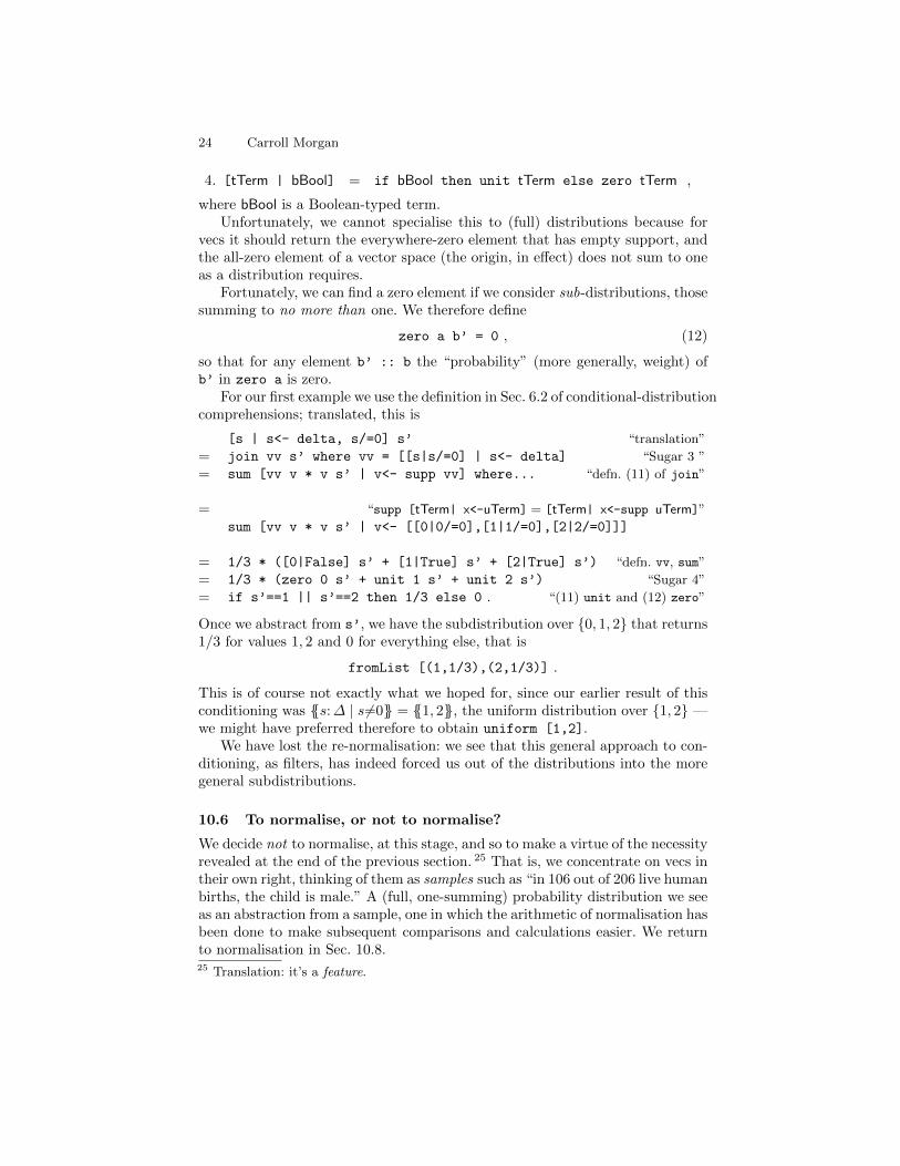
where bBool is a Boolean-typed term.Unfortunately, we cannot specialise this to (full) distributions because for
vecs it should return the everywhere-zero element that has empty support, andthe all-zero element of a vector space (the origin, in effect) does not sum to oneas a distribution requires.
Fortunately, we can find a zero element if we consider sub-distributions, thosesumming to no more than one. We therefore define
zero a b’ = 0 , (12)
so that for any element b’ :: b the “probability” (more generally, weight) ofb’ in zero a is zero.
For our first example we use the definition in Sec. 6.2 of conditional-distributioncomprehensions; translated, this is
[s | s<- delta, s/=0] s’ “translation”
= join vv s’ where vv = [[s|s/=0] | s<- delta] “Sugar 3 ”
= sum [vv v * v s’ | v<- supp vv] where... “defn. (11) of join”
=sum [vv v * v s’ | v<- [[0|0/=0],[1|1/=0],[2|2/=0]]]
“supp [tTerm| x<-uTerm] = [tTerm| x<-supp uTerm]”
= 1/3 * ([0|False] s’ + [1|True] s’ + [2|True] s’) “defn. vv, sum”
= 1/3 * (zero 0 s’ + unit 1 s’ + unit 2 s’) “Sugar 4”
= if s’==1 || s’==2 then 1/3 else 0 . “(11) unit and (12) zero”
Once we abstract from s’, we have the subdistribution over {0, 1, 2} that returns1/3 for values 1, 2 and 0 for everything else, that is
fromList [(1,1/3),(2,1/3)] .
This is of course not exactly what we hoped for, since our earlier result of thisconditioning was {{s:∆ | s6=0}} = {{1, 2}}, the uniform distribution over {1, 2} —we might have preferred therefore to obtain uniform [1,2].
We have lost the re-normalisation: we see that this general approach to con-ditioning, as filters, has indeed forced us out of the distributions into the moregeneral subdistributions.
10.6 To normalise, or not to normalise?
We decide not to normalise, at this stage, and so to make a virtue of the necessityrevealed at the end of the previous section. 25 That is, we concentrate on vecs intheir own right, thinking of them as samples such as “in 106 out of 206 live humanbirths, the child is male.” A (full, one-summing) probability distribution we seeas an abstraction from a sample, one in which the arithmetic of normalisation hasbeen done to make subsequent comparisons and calculations easier. We returnto normalisation in Sec. 10.8.25 Translation: it’s a feature.
An old new notation for elementary probability theory 25
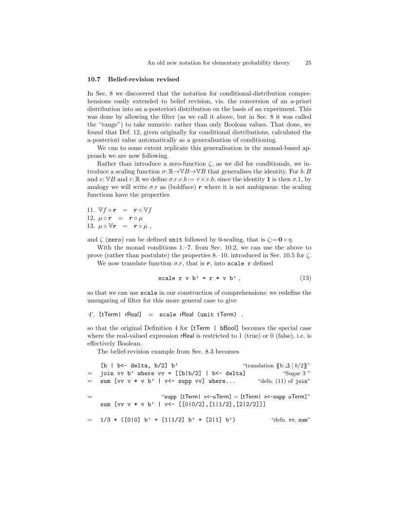
10.7 Belief-revision revised
In Sec. 8 we discovered that the notation for conditional-distribution compre-hensions easily extended to belief revision, vis. the conversion of an a-prioridistribution into an a-posteriori distribution on the basis of an experiment. Thiswas done by allowing the filter (as we call it above, but in Sec. 8 it was calledthe “range”) to take numeric- rather than only Boolean values. That done, wefound that Def. 12, given originally for conditional distributions, calculated thea-posteriori value automatically as a generalisation of conditioning.
We can to some extent replicate this generalisation in the monad-based ap-proach we are now following.
Rather than introduce a zero-function ζ, as we did for conditionals, we in-troduce a scaling function σ:R→VB→VB that generalises the identity. For b:Band v:VB and r:R we define σ.r.v.b := r×v.b; since the identity 1 is then σ.1, byanalogy we will write σ.r as (boldface) r where it is not ambiguous: the scalingfunctions have the properties
11. Vf ◦ r = r ◦ Vf12. µ ◦ r = r ◦ µ13. µ ◦ Vr = r ◦ µ ,
and ζ (zero) can be defined unit followed by 0-scaling, that is ζ:= 0 ◦ η.With the monad conditions 1.–7. from Sec. 10.2, we can use the above to
prove (rather than postulate) the properties 8.–10. introduced in Sec. 10.5 for ζ.We now translate function σ.r, that is r, into scale r defined
scale r v b’ = r * v b’ , (13)
so that we can use scale in our construction of comprehensions: we redefine theunsugaring of filter for this more general case to give
4’. [tTerm| rReal] = scale rReal (unit tTerm) ,
so that the original Definition 4 for [tTerm | bBool] becomes the special casewhere the real-valued expression rReal is restricted to 1 (true) or 0 (false), i.e. iseffectively Boolean.
The belief-revision example from Sec. 8.3 becomes
[b | b<- delta, b/2] b’ “translation {{b:∆ | b/2}}”= join vv b’ where vv = [[b|b/2] | b<- delta] “Sugar 3 ”
= sum [vv v * v b’ | v<- supp vv] where... “defn. (11) of join”
=sum [vv v * v b’ | v<- [[0|0/2],[1|1/2],[2|2/2]]]
“supp [tTerm| x<-uTerm] = [tTerm| x<-supp uTerm]”
= 1/3 * ([0|0] b’ + [1|1/2] b’ + [2|1] b’) “defn. vv, sum”
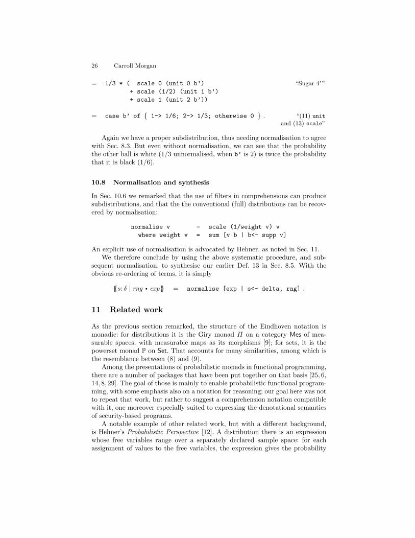
26 Carroll Morgan
= 1/3 * ( scale 0 (unit 0 b’)
+ scale (1/2) (unit 1 b’)
+ scale 1 (unit 2 b’))
“Sugar 4’ ”
= case b’ of { 1-> 1/6; 2-> 1/3; otherwise 0 } . “(11) unit
and (13) scale”
Again we have a proper subdistribution, thus needing normalisation to agreewith Sec. 8.3. But even without normalisation, we can see that the probabilitythe other ball is white (1/3 unnormalised, when b’ is 2) is twice the probabilitythat it is black (1/6).
10.8 Normalisation and synthesis
In Sec. 10.6 we remarked that the use of filters in comprehensions can producesubdistributions, and that the the conventional (full) distributions can be recov-ered by normalisation:
normalise v = scale (1/weight v) v
where weight v = sum [v b | b<- supp v]
An explicit use of normalisation is advocated by Hehner, as noted in Sec. 11.We therefore conclude by using the above systematic procedure, and sub-
sequent normalisation, to synthesise our earlier Def. 13 in Sec. 8.5. With theobvious re-ordering of terms, it is simply
{{s: δ | rng · exp}} = normalise [exp | s<- delta, rng] .
11 Related work
As the previous section remarked, the structure of the Eindhoven notation ismonadic: for distributions it is the Giry monad Π on a category Mes of mea-surable spaces, with measurable maps as its morphisms [9]; for sets, it is thepowerset monad P on Set. That accounts for many similarities, among which isthe resemblance between (8) and (9).
Among the presentations of probabilistic monads in functional programming,there are a number of packages that have been put together on that basis [25, 6,14, 8, 29]. The goal of those is mainly to enable probabilistic functional program-ming, with some emphasis also on a notation for reasoning; our goal here was notto repeat that work, but rather to suggest a comprehension notation compatiblewith it, one moreover especially suited to expressing the denotational semanticsof security-based programs.
A notable example of other related work, but with a different background,is Hehner’s Probabilistic Perspective [12]. A distribution there is an expressionwhose free variables range over a separately declared sample space: for eachassignment of values to the free variables, the expression gives the probability
An old new notation for elementary probability theory 27
of that assignment as an observation: thus for n:N+ the expression 2−n is anexample of a geometric distribution on the positive integers.
With a single new operator l, for normalisation, and existing programming-like notations, Hehner reconstructs many familiar artefacts of probability theory(including conditional distributions and a posteriori analyses), and convincinglydemystifies a number of probability puzzles, including some of those treated here.In Sec. 10.8, also we treated normalisation explicitly.
A strategic difference between our two approaches is (we believe) that Hehner’saim is in part to put elementary probability theory on a simpler, more rationalfooting; we believe he succeeds. In the sense of our comments in Sec. 1, he isworking “forwards.” As we hope Sec. 9 demonstrated, we started instead withexisting probabilistic constructions (essentially Hidden Markov Models as weexplain elsewhere [19]), as a program semantics for noninterference, and thenworked backwards towards the Eindhoven quantifier notation. One of the sensesin which we met Hehner “in the middle” is that we both identify discrete dis-tributions as first-class objects, for Hehner a real-valued expression over freevariables of a type and for us a function from that type into the reals.
In conventional approaches to probability theory that explicit treatment ofdistributions, i.e. giving them names and manipulating them, does not occuruntil one reaches either proper measures or Markov chains. For us it is (in spirit)the former; we believe part of Hehner’s approach can be explained in terms ofthe latter.
A technical difference is our explicit treatment of free- and bound variables,a principal feature of the Eindhoven notation and one reason we chose it.
12 Summary and prospects
We have argued that Eindhoven-style quantifier notation simplifies many of theconstructions appearing in elementary probability. As evidence for this we invitecomparison of the single expression (9) with the paragraphs of Sec. 9.3. We havealso shown how the notation arises naturally from a monadic viewpoint.
There is no space here to give a comprehensive list of calculational identi-ties; but we mention two of them as examples of how the underlying structurementioned above (Sec. 10) generates equalities similar to those already familiarfrom the Eindhoven notation applied to sets.
One identity is the trading rule
(Es: {{s: δ | rng ′ · exp′}} | rng · exp)= (Es: δ | rng ′ × rng [s\exp′] · exp[s\exp′]) ,
(14)
so-called because it “trades” components of an inner quantification into an outerone. Specialised to defaults for true for rng and s for exp′, it gives an alternativeto Def. 11. An identity similar to this took us from (7) to (9).
A second identity is the one used in Sec. 8.4, that (Es: δ; s′: δ′ | rng · exp)
equals (Es: δ | (Es′: δ′ · rng) · exp) when s′ is not free in exp. As noted there, thiscorresponds to a similar trading rule between set comprehension and existential
28 Carroll Morgan
quantification: both are notationally possible only because variable bindings areexplicitly given even when those variables are not used. This is just what theEindhoven style mandates.
The notations here generalise to (non-discrete) probability measures, i.e. evento non-elementary probability theory, again because of the monadic structure.For example the integral of a measurable function given as expression exp in avariable s on a sample space S, with respect to a measure µ, could conventionallybe written
∫exp µ(ds). 26 We write it however as(Es:µ · exp), and have access
to (14)-like identities such as
(Es: {{s′:µ · exp′}} · exp) = (Es′:µ · exp[s\exp]) .
(See App. A for how this would be written conventionally for measures.)We ended in Sec. 9 with an example of how the notation improves the
treatment of probabilistic computer programs, particularly those presented ina denotational-semantic style and based on Hidden Markov Models for quan-titative noninterference security [13, 19]. Although the example concludes thisreport, it was the starting point for the work.
Acknowledgements Jeremy Gibbons identified functional-programmingactivity in this area, and shared his own recent work with us. Frits Vaandragergenerously hosted our six-month stay at Radboud University in Nijmegen during2011. The use of this notation for security (Sec. 9.2) was in collaboration withAnnabelle McIver and Larissa Meinicke [18, 19, and others].
Roland Backhouse, Eric Hehner, Bart Jacobs and David Jansen made manyhelpful suggestions on the original paper; in particular Jansen suggested lookingat continuous distributions (i.e. those given as a density function).
For this revision, I thank members of IFIP WG 2.1, in particular the mem-bers of the “problem-solving group” at the Ottawa meeting (Lambert Meertens,Jeremy Gibbons, Henk Boom, Fritz Henglein), for ideas on how to introduce fil-ters into distribution comprehensions in a monadic way. Separately, Phil Wadlermade many suggestions for Sec. 10, proposing an implementation of the monadwith which he was able to code many of the paper’s examples [29].
Finally, Lambert Meertens wrote extensive and detailed comments on thewhole paper: they were received just the day before the world was due to end.If you are reading this, it did not.
References
1. Thorsten Altenkirch, James Chapman, and Tarmo Uustalu. Monads need not beendofunctors, 2012. Available atciteseerx.ist.psu.edu/viewdoc/summary?doi=10.1.1.156.7931.
26 Or not? We say “could” because “[there] are a number of different notations for theintegral in the literature; for instance, one may find any of the following:
∫Ysdµ,∫
Ys(x) dµ,
∫Ys(x)µ,
∫Ys(x)µ( dx), or even
∫Ys(x) dx. . . ” [2].

An old new notation for elementary probability theory 29
2. Steve Cheng. A crash course on the Lebesgue integral and measure theory.www.gold-saucer.org/math/lebesgue/lebesgue.pdf, downloaded Dec. 2011.
3. Y. Deng, R. van Glabbeek, M. Hennessy, C.C. Morgan, and C. Zhang. Character-ising testing preorders for finite probabilistic processes. In Proc LiCS 07, 2007.
4. E.W. Dijkstra. A Discipline of Programming. Prentice-Hall, 1976.
5. E.W. Dijkstra and C.S. Scholten. Predicate Calculus and Program Semantics.Springer, 1990.
6. Martin Erwig and Steve Kollmansberger. Probabilistic functional programming inHaskell. Journal of Functional Programming, 16:21–34, 2006.
7. D.H. Fremlin. Measure Theory. Torres Fremlin, 2000.
8. Jeremy Gibbons and Ralf Hinze. Just do it: simple monadic equational reasoning.In Manuel M. T. Chakravarty, Zhenjiang Hu, and Olivier Danvy, editors, ICFP,pages 2–14. ACM, 2011.
9. M. Giry. A categorical approach to probability theory. In Categorical Aspects ofTopology and Analysis, volume 915 of Lecture Notes in Mathematics, pages 68–85.Springer, 1981.
10. J.A. Goguen and J. Meseguer. Unwinding and inference control. In Proc. IEEESymp on Security and Privacy, pages 75–86. IEEE Computer Society, 1984.
11. Ian Hayes. Specification Case Studies. Prentice-Hall, 1987.http://www.itee.uq.edu.au/∼ianh/Papers/SCS2.pdf.
12. Eric C. R. Hehner. A probability perspective. Form. Asp. Comput., 23:391–419,July 2011.
13. D. Jurafsky and J.H. Martin. Speech and Language Processing. Prentice HallInternational, 2000.
14. Oleg Kiselyov and Chung-Chieh Shan. Embedded probabilistic programming. InWalid Taha, editor, Domain-Specific Languages, volume 5658 of Lecture Notes inComputer Science, pages 360–384. Springer, 2009.
15. E Kowalski. Measure and integral.www.math.ethz.ch/∼kowalski/measure-integral.pdf, downloaded Dec. 2011.
16. F.W. Lawvere. The category of probabilistic mappings, 1962. (Preprint).
17. A.K. McIver and C.C. Morgan. Abstraction, Refinement and Proof for ProbabilisticSystems. Tech Mono Comp Sci. Springer, New York, 2005.
18. Annabelle McIver, Larissa Meinicke, and Carroll Morgan. Compositional closurefor Bayes Risk in probabilistic noninterference. In Proceedings of the 37th interna-tional colloquium conference on Automata, languages and programming: Part II,volume 6199 of ICALP’10, pages 223–235, Berlin, Heidelberg, 2010. Springer.
19. Annabelle McIver, Larissa Meinicke, and Carroll Morgan. Hidden-Markov pro-gram algebra with iteration. At arXiv:1102.0333v1; to appear in MathematicalStructures in Computer Science in 2012, 2011.
20. Annabelle McIver, Larissa Meinicke, and Carroll Morgan. A Kantorovich-monadicpowerdomain for information hiding, with probability and nondeterminism. InProc. LiCS 2012, 2012.
21. Carroll Morgan. Compositional noninterference from first principles. Formal As-pects of Computing, pages 1–24, 2010. 10.1007/s00165-010-0167-y.
22. C.C. Morgan. The Shadow Knows: Refinement of ignorance in sequential programs.In T. Uustalu, editor, Math Prog Construction, volume 4014 of Springer, pages359–78. Springer, 2006. Treats Dining Cryptographers.
23. C.C. Morgan. The Shadow Knows: Refinement of ignorance in sequential programs.Science of Computer Programming, 74(8):629–653, 2009. Treats Oblivious Transfer.
30 Carroll Morgan
24. C.C. Morgan, A.K. McIver, and K. Seidel. Probabilistic predicate transformers.ACM Trans Prog Lang Sys, 18(3):325–53, May 1996.doi.acm.org/10.1145/229542.229547.
25. Norman Ramsey and Avi Pfeffer. Stochastic lambda calculus and monads of prob-ability distributions. SIGPLAN Not., 37:154–165, January 2002.
26. Haskell Report. www.haskell.org/onlinereport/haskell2010/, 2010.27. G. Smith. Adversaries and information leaks (Tutorial). In G. Barthe and C. Four-
net, editors, Proc. 3rd Symp. Trustworthy Global Computing, volume 4912 of LNCS,pages 383–400. Springer, 2007.
28. Philip Wadler. Comprehending monads. In Mathematical Structures in ComputerScience, pages 61–78, 1992.
29. Philip Wadler. Private communication. 2013.
An old new notation for elementary probability theory 31
Appendices
A Measure spaces
More general than discrete distributions, measures are used for probability overinfinite sample spaces, where expected value becomes integration [7]. Here wesketch how “measure comprehensions” might appear; continuous distributionswould be a special case of those.
In Riemann integration we write∫ bax2 dx for the integral of the real-valued
squaring-function sqr := (λx · x2) over the interval [a, b], and in that notationthe x in x2 is bound by the quantifier dx. The scope of the binding is from
∫to dx.
In Lebesgue integration however we write∫
sqr dµ for the integral of thatsame function over a measure µ.
The startling difference between those two notations is the use of of theconcrete syntax “d” that in Riemann integration’s dx binds x, while for measuresthe µ in dµ is free. To integrate the expression form of the squaring-function overµ we have to bind its x in another way: two typical approaches are
∫x2 µ(dx)
and∫x2 dµ(x) [2]. 27
An alternative is to achieve some uniformity by using d(·) in the same wayfor both kinds of integrals [17]. We use
∫exp dx for
∫(λx · exp) in all cases; and
the measure, or the bounds, are always found outside the expression, next to theintegral sign
∫. Thus we write
∫µ(·) for integration over general measure µ, and
then the familiar∫ ba
(·) is simply a typographically more attractive presentationof the special case
∫[a,b]
(·) over the uniform measure on the real interval [a, b]. 28
Then with f := (λx · F ) we would have the equalities∫{{c}}F dx =
∫{{c}}f = f.c one-point rule
and
∫g∗.µ
F dx =
∫g∗.µ
f =
∫µ
f◦g recall push-forwardfrom Sec. 5.3.
In the second case we equate the integral of f , over an (unnamed) measureformed by pushing function g forward over measure µ, with the integral of thefunctional composition f◦g over measure µ directly.
For complicated measures, unsuitable as subscripts, an alternative for theintegral notation
∫µ
exp dx is the expected value (Ex:µ · exp). The one-point
rule is then written (Ex: {{exp}} · F ) = F [x\exp]. In the second case we have
(Ex: {{y:µ · G}} · F ) = (Ey:µ · F [x\G]) , (15)
27 And there are more, since “[if] we want to display the argument of the integrandfunction, alternate notations for the integral include
∫x∈X f(x) dµ. . . ” [15].
28 This is more general than probabiity measures, since the (e.g. Lebesgue) measureb−a of the whole interval [a, b] can exceed one.

32 Carroll Morgan
where function g has become the lambda abstraction (λy · G). In Lem. 3 belowwe prove (15) for the discrete case.
B Exploiting non-freeness in the constructor
Here we prove the nontrivial step referred forward from Sec. 8.4: the main as-sumption is that s′ is not free in exp. But should δ itself be an expression, werequire that s′ not be free there either.
(Es: δ; s′: δ′ | rng · exp)= (Es: δ; s′: δ′ · rng × exp) / (Es: δ; s′: δ′ · rng) “Def. 11”
=(Σs:S; s′:S′ · δ.s× δ′.s′ × rng × exp)
(Σs:S; s′:S′ · δ.s× δ′.s′ × rng)“Def. 7”
=(Σs:S · δ.s× (Σs′:S′ · δ′.s′ × rng)× exp)
(Σs:S · δ.s× (Σs′:S′ · δ′.s′ × rng))“s′ not free in exp”
= (Es: δ · (Es′: δ′ · rng)× exp) / (Es: δ · (Es′: δ′ · rng)) “Def. 7”
= (Es: δ | (Es′: δ′ · rng) · exp) . “Def. 11”
C Assorted proofs related to definitions 29
Lemma 1. {{s: δ · exp}} is a distribution on {s: dδe · exp}Proof: We omit the simple proof that 0≤{{s: δ · exp}}; for the one-summing
property, we write S for dδe and calculate
(Σe: {s:S · exp} · {{s: δ · exp}}.e) “let e be fresh”
= (Σe: {s:S · exp} · (Es: δ · [exp=e])) “Def. 9”
= (Σe: {s:S · exp} · (Σs:S · δ.s×[exp=e])) “Def. 7”
= (Σs:S; e: {s:S · exp} · δ.s×[exp=e]) “merge and swap summations”
= (Σs:S; e: {s:S · exp} | exp=e · δ.s) “trading”
= (Σs:S · δ.s) “one-point rule”
= 1 . “δ is a distribution”
2
Lemma 2. {{s: δ | rng}} is a distribution on dδe if (Es: δ · rng)6=0
Proof: We omit the simple proof that 0≤{{s: δ | rng}}; for the one-summingproperty, we write S for dδe and calculate
29 We thank Roland Backhouse for the suggestion to include the first two of these.
An old new notation for elementary probability theory 33
(Σs′:S · {{s: δ | rng}}.s′) “let s′ be fresh”
= (Σs′:S · (Es: δ · rng × [s=s′]) / (Es: δ · rng)) “Def. 10”
= (Σs′:S · (Es: δ · rng × [s=s′])) / (Es: δ · rng) “s′ not free in denominator”
= (Es: δ · rng) / (Es: δ · rng) “one-point rule; Def. 7”
= 1 . “(Es: δ · rng) 6=0”
2
Lemma 3. (Ex: {{y: δ · G}} · F ) = (Ey: δ · F [x\G])
This is Equation (15) in the discrete case.
Proof: Let X be the support of {{y: δ · G}}, for which a more concisenotation is given in App. D below, and let Y be the support of δ; we calculate
(Ex: {{y: δ · G}} · F )= (Σx:X · {{y: δ · G}}.x× F ) “Def. 7”
= (Σx:X · (Ey: δ · [G=x])× F ) “Def. 9”
= (Σx:X · (Σy:Y · δ.y × [G=x])× F ) “Def. 7”
= (Σy:Y ;x:X · δ.y × [G=x]× F ) “distribution of summations”
= (Σy:Y · δ.y × F [x\G]) “one-point rule for summation”
= (Ey: δ · F [x\G]) . “Def. 7”
2
From Lem. 3 we have immediately an analogous equality for distributions,since distribution comprehensions are a special case of expected values: a moresuccinct, point-free alternative to Def. 9 and Def. 13 is given by the equality
{{s: δ | rng · exp}} = (Es: δ | rng · {{exp}}) , 30 (16)
where the right-hand expected value is being taken in a vector space (of discretedistributions). This is how we simplified (7) to (9) in Sec. 9.
D Further identities
The identities below are motivated by the first one, i.e. Sec. D.1, justifying theidea that in a comprehension with both range and constructor one can think interms of enforcing the range as a first step, and then the constructor to whatresults. The identities are listed in order of increasing generality.
For conciseness in this section we use Enewold for substitution
and letters R,E instead of words rng , exp for expressionsand ds: δ | rng · expe for the support d{{s: δ | rng · exp}}e.
30 from (Es: δ | rng · {{exp}}).e = (Es: δ | rng · {{exp}}.e) = (Es: δ | rng · [exp=e]) .

34 Carroll Morgan
D.1 —————————
(Es: {{s: δ | R}} · E)= (Ee: {{s: δ | R}} · Ees) “fresh variable e”
= (Σe: ds: δ | Re · {{s: δ | R}}.e× Ees)= (Σe: ds: δ | Re · (Es: δ | R · [s=e])× Ees)= (Σe: ds: δ | Re · (Es: δ · R× [s=e])× Ees/(Es: δ · R))= (Σe: ds: δ | Re · δ.e×Res × Ees/(Es: δ · R)) “one-point rule”
= (Σe: ds: δ | Re · δ.e×Res × Ees)/(Es: δ · R) “e not free in R or δ”
= (Ee: δ · Res × Ees)/(Es: δ · R) “definition E and ds: δ | Re”= (Es: δ · R× E)/(Es: δ · R) “e not free in R,E”
= (Es: δ | R · E) . “Def. 11”
D.2 ————————— D.1 for distributions
{{s: {{s: δ | R}} · E}}= {{s: δ | R · E}} . “from Sec. D.1 under the same conditions, using (16)”
D.3 —————————
An elaboration of Sec. D.1 with constructor F , generalising Lem. 3.
(Es: {{s: δ | R · F}} · E)=
(Σe: ds: δ | R · F e · (Es: δ · R× [F=e])× Ees/(Es: δ · R))“as for Sec. D.1. . . ”
=(Σe: ds: δ | R · F e · (Σs: dδe · δ.s×R× [F=e])× Ees/(Es: δ · R))
“. . . but cannot use one-point wrt. F”
= (Σs: dδe; e: ds: δ | R · F e · δ.s×R× [F=e]× Ees/(Es: δ · R))
= (Σs: dδe · δ.s×R× EFs /(Es: δ · R)) “if δ.s and R both nonzero,then F∈ds: δ | R · F e;
e not free in R”
= (Σs: dδe · δ.s×R× EFs )/(Es: δ · R)= (Es: δ · R× EFs )/(Es: δ · R)= (Es: δ | R · EFs ) .
D.4 ————————— D.3 for distributions
{{s: {{s: δ | R · F}} · E}}= {{s: δ | R · EFs }} . “from Sec. D.3, under the same conditions”
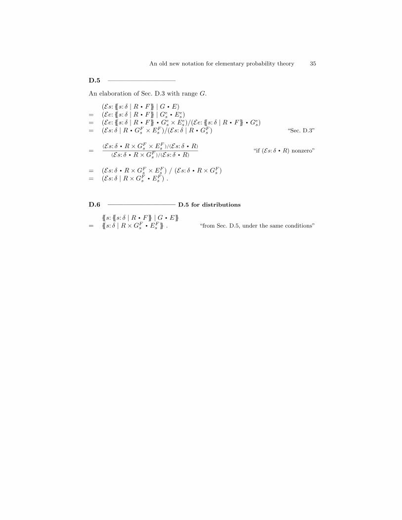
An old new notation for elementary probability theory 35
D.5 —————————
An elaboration of Sec. D.3 with range G.
(Es: {{s: δ | R · F}} | G · E)= (Ee: {{s: δ | R · F}} | Ges · Ees)= (Ee: {{s: δ | R · F}} · Ges × Ees)/(Ee: {{s: δ | R · F}} · Ges)= (Es: δ | R · GFs × EFs )/(Es: δ | R · GFs ) “Sec. D.3”
=(Es: δ · R×GFs × EFs )/(Es: δ · R)
(Es: δ · R×GFs )/(Es: δ · R)“if (Es: δ · R) nonzero”
= (Es: δ · R×GFs × EFs ) / (Es: δ · R×GFs )= (Es: δ | R×GFs · EFs ) .
D.6 ————————— D.5 for distributions
{{s: {{s: δ | R · F}} | G · E}}= {{s: δ | R×GFs · EFs }} . “from Sec. D.5, under the same conditions”