An Observing System Simulation Experiment for the Calibration andValidation of the Surface Water Ocean Topography Sea Surface

Height Measurement Using In Situ Platforms

JINBO WANG,a LEE-LUENG FU,a BO QIU,b DIMITRIS MENEMENLIS,a J. THOMAS FARRAR,c YI CHAO,d

ANDREW F. THOMPSON,e AND MAR M. FLEXASe

a Jet Propulsion Laboratory, California Institute of Technology, Pasadena, CaliforniabUniversity of Hawai‘i at M�anoa, Honolulu, Hawaii

cWoods Hole Oceanographic Institution, Woods Hole, MassachusettsdRemote Sensing Solutions, Monrovia, California

eCalifornia Institute of Technology, Pasadena, California

(Manuscript received 18 April 2017, in final form 16 October 2017)

ABSTRACT

The wavenumber spectrum of sea surface height (SSH) is an important indicator of the dynamics of the

ocean interior. While the SSH wavenumber spectrum has been well studied at mesoscale wavelengths and

longer, using both in situ oceanographic measurements and satellite altimetry, it remains largely unknown for

wavelengths less than ;70 km. The Surface Water Ocean Topography (SWOT) satellite mission aims to

resolve the SSH wavenumber spectrum at 15–150-km wavelengths, which is specified as one of the mission

requirements. The mission calibration and validation (CalVal) requires the ground truth of a synoptic SSH

field to resolve the targeted wavelengths, but no existing observational network is able to fulfill the task. A

high-resolution global ocean simulation is used to conduct an observing system simulation experiment

(OSSE) to identify the suitable oceanographic in situ measurements for SWOT SSH CalVal. After fixing 20

measuring locations (the minimum number for resolving 15–150-km wavelengths) along the SWOT swath,

four instrument platforms were tested: pressure-sensor-equipped inverted echo sounders (PIES), underway

conductivity–temperature–depth (UCTD) sensors, instrumented moorings, and underwater gliders. In the

context of the OSSE, PIES was found to be an unsuitable tool for the target region and for SSH scales 15–

70 km; the slowness of a single UCTD leads to significant aliasing by high-frequency motions at short

wavelengths below ;30 km; an array of station-keeping gliders may meet the requirement; and an array of

moorings is the most effective system among the four tested instruments for meeting the mission’s re-

quirement. The results shown here warrant a prelaunch field campaign to further test the performance of

station-keeping gliders.

1. Introduction

The Surface Water Ocean Topography (SWOT)

mission aims to measure both the land water and ocean

topography with an unprecedented horizontal resolu-

tion. The mission’s satellite will carry a Ka-band Radar

Interferometer (KaRIN) designed to yield high spatial

resolutions over two swaths of 50 km with a 20-km gap

centered at the nadir track (Durand et al. 2010; Fu and

Ubelmann 2014). This paper focuses only on the ocean

component. The high-resolution two-dimensional ocean

topography measurements will enable us to study the

upper-ocean dynamics and the associated heat and

tracer transports therein, which are important processes

in the climate system (Klein et al. 2015).

We are interested in the sea surface height (SSH)

component that was governed by ocean eddies and high-

frequency internal waves (referred to as steric height and

explained in section 4). As a result, the steric height is

referred to as the ground truth. It is shown in section 5c

that after removing the atmospheric loading and the

barotropic signals reflected in the bottom pressure, the

sea surface height measured by satellite is equivalent to

the steric height. The measurement error is conse-

quently defined as the difference between satellite

measurements (after the inverted barometer and baro-

tropic tidal corrections) and steric height in this paper.Corresponding author: Dr. Jinbo Wang, jinbo.wang@jpl.nasa.

gov

FEBRUARY 2018 WANG ET AL . 281

DOI: 10.1175/JTECH-D-17-0076.1

� 2018 American Meteorological Society. For information regarding reuse of this content and general copyright information, consult the AMS CopyrightPolicy (www.ametsoc.org/PUBSReuseLicenses).

For the first time, the mission’s requirement is

specified in terms of the cross-track averaged wave-

number spectrum of measurement errors (Fig. 1). The

baseline error requirement (the red line in Fig. 1) is an

approximation of the summation of all the noises and

errors, including a constant white noise that dominates

at small wavelengths and a colored noise that repre-

sents residual geophysical errors, orbit errors, and at-

titude restitution errors, and that dominates at longer

wavelengths. More details can be found in the SWOT

science requirements document (Rodríguez 2016).

This unprecedented mission requirement in the wave-

number space imposes challenges on the SSH calibra-

tion and validation (SSH CalVal) task. While the

onboard conventional nadir altimeter can be used for

wavelengths longer than 150 km (appendix A), the SSH

CalVal becomes more complex at 15–150 km (also re-

ferred to as the SWOT scales) because of the presence

of high-frequency oceanic motions. It is therefore

crucial to provide the ground truth for the steric height

at the SWOT scales for the CalVal purpose.

While it is theoretically simple to reconstruct the

steric height from ocean interior temperature T

and salinity S measurements, no existing observa-

tional network can provide a synoptic wavenumber

spectrum at these wavelengths. Here we perform an

observing system simulation experiment (OSSE)

using a high-resolution global ocean simulation to

help design a new observing system to fulfill the mis-

sion’s requirement.

We focus on resolving 15–150-km wavelengths. The

shortest wavelength 15 km requires the minimum

measurement resolution to be 7.5 km (resolve 15 km

as the Nyquist wavelength). To resolve the longest

wavelength (150 km), we need to have 20 points of

measurements, given that the distance between

measurements is determined by the Nyquist wave-

length, that is, 150 km/7.5 km5 20. Here we regard 20

measuring locations along the swath as the baseline

configuration. We selected four oceanographic in-

struments that can perform the SSH reconstruction,

either from direct measurements of ocean interior T/S

or from a proxy that is correlated to steric heights (see

section 4). The pressure-sensor-equipped inverted

echo sounder (PIES) reconstructs the steric height

using an empirical relationship between the time for

an acoustic pulse to travel through the water column

and the steric height itself. Underway conductivity–

temperature–depth (UCTD), moorings with CTDs,

and gliders can directly measure T/S profiles to re-

trieve the steric height.

The outline of the paper is as follows. In section 2

we discuss the SWOT CalVal orbit and the two

potential CalVal sites. Section 3 includes descriptions

of the numerical simulation used as a representation of

the true SSH (the ‘‘nature run’’). In section 4 we discuss

the basis for reconstructing the steric height in the

nature run and the characteristics of the steric height

variability therein. In section 5 we describe the OSSE

methodology, including the description of the simula-

tion of the four instruments and the synthetic SWOT

SSH. Since PIES and UCTD are found to be in-

adequate in meeting the CalVal requirement, we focus

onmoorings and gliders. Results are shown in section 6,

where we diagnose SSH from the simulated glider and

mooring measurements. Discussion and conclusions

are presented in section 7.

2. The SWOT orbit and two potential sites forCalVal

The SWOT CalVal will occur during the 90-day

calibration phase in a one-day repeat orbit (Fig. 2)

after the instrument checkout phase when the

onboard configuration of the instruments has been

settled (Fu et al. 2012). This fast sampling phase sig-

nificantly expedites the data acquisition for the in-

strument calibration and its performance validation,

and it minimizes the calibration time for the transition

to the nominal mission phase. The 1-day repeat fast

sampling increases the temporal resolution at the cost

FIG. 1. SSH baseline requirement spectrum (red curve) as

a function of wavenumber represented by an empirical function

E(k)5 21 0:001 25k22, where k represents the wavenumber, and

the threshold requirement (blue curve). Shown for reference is the

global mean SSH spectrum estimated from the Jason-1 and Jason-2

observations (thick black line), the lower boundary of 68% of the

spectral values (thin black line), and the lower boundary of 95% of

the spectral values (gray line). Intersections of the two dotted lines

with the baseline spectrum at ;15 km (68%) and ;30 km (95%)

determine the resolving capabilities of the SWOT measurement.

Respective resolutions for the threshold requirement are ;25 km

(68%) and ;35 km (95%) (Rodríguez 2016).

282 JOURNAL OF ATMOSPHER IC AND OCEAN IC TECHNOLOGY VOLUME 35

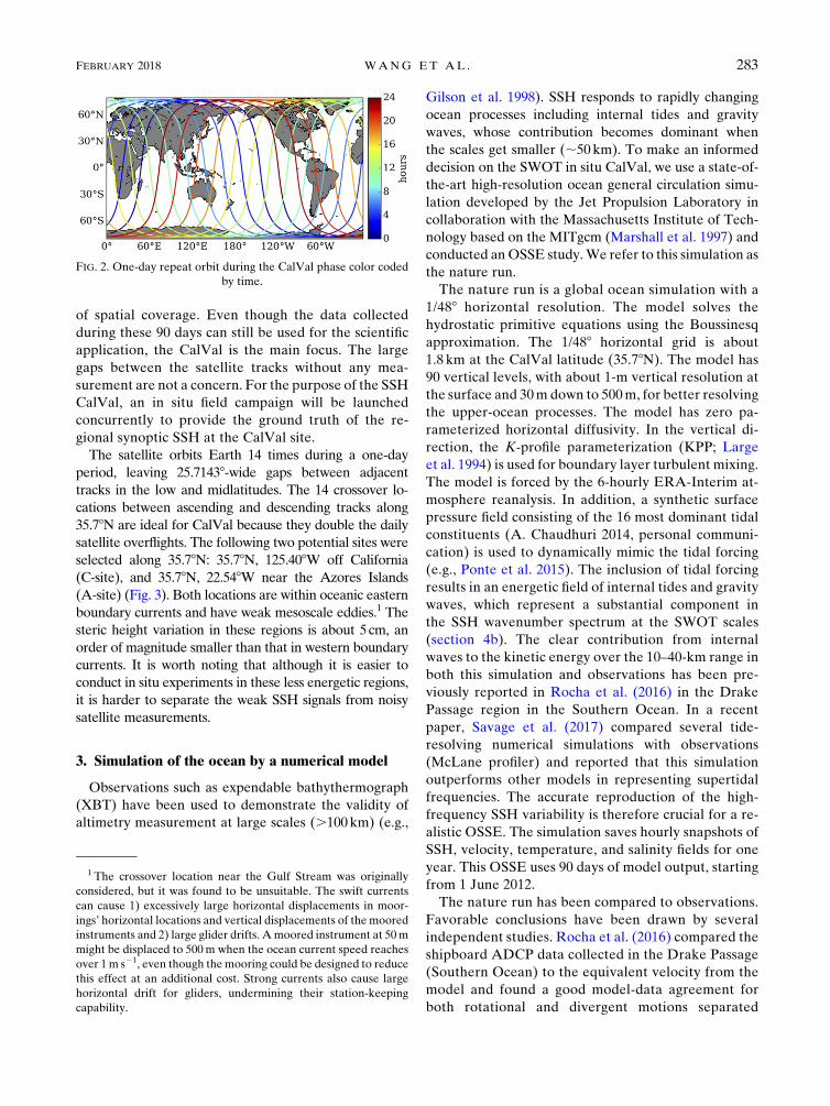
of spatial coverage. Even though the data collected

during these 90 days can still be used for the scientific

application, the CalVal is the main focus. The large

gaps between the satellite tracks without any mea-

surement are not a concern. For the purpose of the SSH

CalVal, an in situ field campaign will be launched

concurrently to provide the ground truth of the re-

gional synoptic SSH at the CalVal site.

The satellite orbits Earth 14 times during a one-day

period, leaving 25.71438-wide gaps between adjacent

tracks in the low and midlatitudes. The 14 crossover lo-

cations between ascending and descending tracks along

35.78N are ideal for CalVal because they double the daily

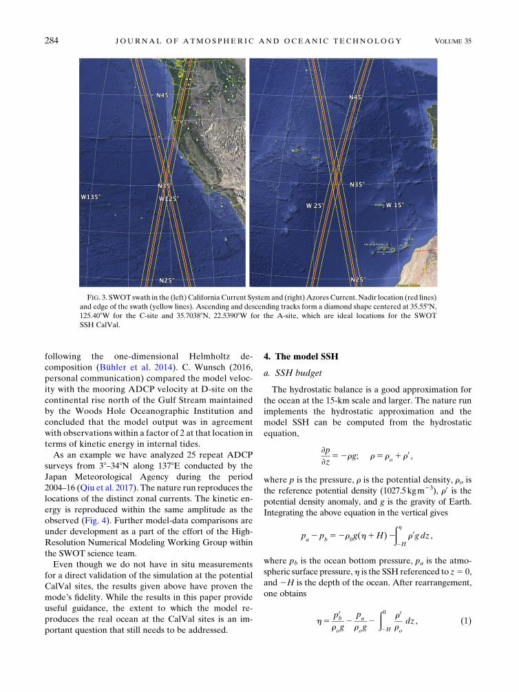
satellite overflights. The following two potential sites were

selected along 35.78N: 35.78N, 125.408W off California

(C-site), and 35.78N, 22.548W near the Azores Islands

(A-site) (Fig. 3). Both locations are within oceanic eastern

boundary currents and have weak mesoscale eddies.1 The

steric height variation in these regions is about 5cm, an

order of magnitude smaller than that in western boundary

currents. It is worth noting that although it is easier to

conduct in situ experiments in these less energetic regions,

it is harder to separate the weak SSH signals from noisy

satellite measurements.

3. Simulation of the ocean by a numerical model

Observations such as expendable bathythermograph

(XBT) have been used to demonstrate the validity of

altimetry measurement at large scales (.100 km) (e.g.,

Gilson et al. 1998). SSH responds to rapidly changing

ocean processes including internal tides and gravity

waves, whose contribution becomes dominant when

the scales get smaller (;50 km). To make an informed

decision on the SWOT in situ CalVal, we use a state-of-

the-art high-resolution ocean general circulation simu-

lation developed by the Jet Propulsion Laboratory in

collaboration with the Massachusetts Institute of Tech-

nology based on the MITgcm (Marshall et al. 1997) and

conducted anOSSE study.We refer to this simulation as

the nature run.

The nature run is a global ocean simulation with a

1/488 horizontal resolution. The model solves the

hydrostatic primitive equations using the Boussinesq

approximation. The 1/488 horizontal grid is about

1.8 km at the CalVal latitude (35.78N). The model has

90 vertical levels, with about 1-m vertical resolution at

the surface and 30m down to 500m, for better resolving

the upper-ocean processes. The model has zero pa-

rameterized horizontal diffusivity. In the vertical di-

rection, the K-profile parameterization (KPP; Large

et al. 1994) is used for boundary layer turbulent mixing.

The model is forced by the 6-hourly ERA-Interim at-

mosphere reanalysis. In addition, a synthetic surface

pressure field consisting of the 16 most dominant tidal

constituents (A. Chaudhuri 2014, personal communi-

cation) is used to dynamically mimic the tidal forcing

(e.g., Ponte et al. 2015). The inclusion of tidal forcing

results in an energetic field of internal tides and gravity

waves, which represent a substantial component in

the SSH wavenumber spectrum at the SWOT scales

(section 4b). The clear contribution from internal

waves to the kinetic energy over the 10–40-km range in

both this simulation and observations has been pre-

viously reported in Rocha et al. (2016) in the Drake

Passage region in the Southern Ocean. In a recent

paper, Savage et al. (2017) compared several tide-

resolving numerical simulations with observations

(McLane profiler) and reported that this simulation

outperforms other models in representing supertidal

frequencies. The accurate reproduction of the high-

frequency SSH variability is therefore crucial for a re-

alistic OSSE. The simulation saves hourly snapshots of

SSH, velocity, temperature, and salinity fields for one

year. This OSSE uses 90 days of model output, starting

from 1 June 2012.

The nature run has been compared to observations.

Favorable conclusions have been drawn by several

independent studies. Rocha et al. (2016) compared the

shipboard ADCP data collected in the Drake Passage

(Southern Ocean) to the equivalent velocity from the

model and found a good model-data agreement for

both rotational and divergent motions separated

FIG. 2. One-day repeat orbit during the CalVal phase color coded

by time.

1 The crossover location near the Gulf Stream was originally

considered, but it was found to be unsuitable. The swift currents

can cause 1) excessively large horizontal displacements in moor-

ings’ horizontal locations and vertical displacements of the moored

instruments and 2) large glider drifts. Amoored instrument at 50m

might be displaced to 500m when the ocean current speed reaches

over 1m s21, even though the mooring could be designed to reduce

this effect at an additional cost. Strong currents also cause large

horizontal drift for gliders, undermining their station-keeping

capability.

FEBRUARY 2018 WANG ET AL . 283

following the one-dimensional Helmholtz de-

composition (Bühler et al. 2014). C. Wunsch (2016,

personal communication) compared the model veloc-

ity with the mooring ADCP velocity at D-site on the

continental rise north of the Gulf Stream maintained

by the Woods Hole Oceanographic Institution and

concluded that the model output was in agreement

with observations within a factor of 2 at that location in

terms of kinetic energy in internal tides.

As an example we have analyzed 25 repeat ADCP

surveys from 38–348N along 1378E conducted by the

Japan Meteorological Agency during the period

2004–16 (Qiu et al. 2017). The nature run reproduces the

locations of the distinct zonal currents. The kinetic en-

ergy is reproduced within the same amplitude as the

observed (Fig. 4). Further model-data comparisons are

under development as a part of the effort of the High-

Resolution Numerical Modeling Working Group within

the SWOT science team.

Even though we do not have in situ measurements

for a direct validation of the simulation at the potential

CalVal sites, the results given above have proven the

mode’s fidelity. While the results in this paper provide

useful guidance, the extent to which the model re-

produces the real ocean at the CalVal sites is an im-

portant question that still needs to be addressed.

4. The model SSH

a. SSH budget

The hydrostatic balance is a good approximation for

the ocean at the 15-km scale and larger. The nature run

implements the hydrostatic approximation and the

model SSH can be computed from the hydrostatic

equation,

›p

›z52rg; r5 r

o1 r0 ,

where p is the pressure, r is the potential density, ro is

the reference potential density (1027.5kgm23), r0 is thepotential density anomaly, and g is the gravity of Earth.

Integrating the above equation in the vertical gives

pa2 p

b52r

0g(h1H)2

ðh2H

r0g dz ,

where pb is the ocean bottom pressure, pa is the atmo-

spheric surface pressure,h is the SSH referenced to z5 0,

and 2H is the depth of the ocean. After rearrangement,

one obtains

h5p0b

rog2

pa

rog2

ð02H

r0

ro

dz , (1)

FIG. 3. SWOT swath in the (left) California Current System and (right)Azores Current. Nadir location (red lines)

and edge of the swath (yellow lines). Ascending and descending tracks form a diamond shape centered at 35.558N,

125.408W for the C-site and 35.70388N, 22.53908W for the A-site, which are ideal locations for the SWOT

SSH CalVal.

284 JOURNAL OF ATMOSPHER IC AND OCEAN IC TECHNOLOGY VOLUME 35

where pb0 5def

pb 2 gr0H represents the bottom pressure

anomaly, and the termÐ h0(r0/r0) dz has been neglected

because h � H. The three terms on the right-hand side

of Eq. (1) represent the contributions from the bottom

pressure (hb), the atmospheric pressure loading [the

inverted barometer (IB) effect ha], and the steric height

(j, related to dynamic height by a factor of g), re-

spectively. In the following, we use jz12z2 to denote the

steric height as a result of the water column sandwiched

between depths at z1 and z2. For example, j02500 rep-

resents the steric height as a result of the upper 500m.

One necessary verification of the model’s fidelity in

simulating SSH is to check the SSH balance in Eq. (1).

Checking the balance also helps us understand the

dominant factors that modulate SSH signals.

Figure 5 shows the time series of each term in

Eq. (1) sampled near the C-site. At high frequencies, the

dominant terms are between h and hb, mainly reflecting

the high-frequency barotropic signals on the order of

O(102) cm. At subinertial frequencies, all the low-pass

filtered terms are largely reduced in amplitude. The SSH

budget mainly reflects the IB effect (blue and cyan

lines). The steric height j02H is approximatelyO(5) cm.

The hb is reduced to a negligible level at about 5% of the

steric height on the SWOT scales (green line). The

residual (gray line) is almost zero, indicating the closed

SSH budget in the model within the hydrostatic

approximation.

The barotropic signals, the IB effect, and bottom

pressure signals, even though of large amplitude, can be

easily removed using a spatial filter as a result of their

large-scale characteristics. We will discuss this point in

section 5c.

b. The influence of inertia-gravity waves on SSH

The complexity of the SWOT ocean CalVal is mainly

caused by the high-frequency energetic inertia-gravity

waves on the SWOT scales (15–150 km). Our knowledge

of SSH wavenumber spectra is mostly derived from

satellite altimetry available during the past decades,

which is unfortunately dominated by noise at wave-

lengths less than ;100 km (Xu and Fu 2012). While

observations have been used to study the wavenumber

spectra of kinetic/potential energy and tracer variance

(Katz 1973; Samelson and Paulson 1988; Ferrari and

Rudnick 2000; Wang et al. 2010; Callies and Ferrari

2013; Rocha et al. 2016), the wavenumber spectra of

SSH at the SWOT scales are poorly known.

A few recent studies based on numerical simulations

have shown that the inertia-gravity waves have a clear

FIG. 4. Latitude–depth sections of time-mean zonal velocity (colored contours) and density

(black contours in u) along 1378E from (a) JMA repeat ADCP surveys of 2004–16 and (b) the

nature run. Note that contour scales are nonlinear and that colors denote east (red) and

westward (blue) flows.

FEBRUARY 2018 WANG ET AL . 285

contribution to SSH over the SWOT scales (Richman

et al. 2012; Rocha et al. 2016). The SSH wavenumber

spectrum near the C-site in the nature run is shown here

as an example (Fig. 6). The super- and subinertial

components are taken to approximate the wave motions

and the balanced motions, respectively. It is clear that

waves are much more energetic than balanced motions

over a major part of the SWOT scales at this location.

This wave dominance on the submesoscale scale kinetic

energy over the tested regions is not likely a model ar-

tifact considering several recent studies based onADCP

velocity observations also report similar wave domi-

nance in kinetic energy wavenumber spectra (Qiu

et al. 2017).

These energetic high-frequency waves impose diffi-

culty in capturing synoptic SSH signal and warrant high-

frequency sampling strategies, which eliminate the

usage of the platforms that cannot cover a 150-km dis-

tance within a short period of time. Based on the sen-

sitivity studies (results not shown), we conclude that we

need to measure the 150-km distance within about 1 h to

capture the synoptic dynamics.

c. The upper-ocean dominance in SSH variability

We use the following index to measure the contribu-

tion of the upper ocean:

r(z, k)5 12Sjz2Hjz2H

(k)

Sj02Hj02H

(k),

where Sxx(k) represents the power spectrum density of x

as a function of wavenumber k, jz2H represents the steric

height as a result of the water column sandwiched be-

tween z and H. Consequently, r(z0, k0)5 1 means that

j02z0 can explain 100% the full-depth steric height j02H

at k0, or equivalently the ocean beneath z0 has no con-

tribution to the steric height anomaly. One caveat is that

jz2H sometimes has a strong negative correlation with

j02z, so they compensate each other and either of the

two can exceed j02H , resulting in r, 0. The negative

correlation can be understood as the anticorrelation

between the density anomalies of the upper (0–z) and

the lower (z–H) layers. It is a possibility, but it does not

occur in our case. The r(z, k) at the C-site is .70% for

all wavenumbers if z,2580m (Fig. 7), indicating the

upper-ocean dominance in the steric height component

of the SSH. However, it is still a question whether the

remaining 30% signal leads to errors larger than the

CalVal requirement.

FIG. 6. Wavenumber spectrum of the hourly h (green) and the low-

pass filtered (.24 h) version (blue).

FIG. 5. Time series of each term in Eq. (1): h (blue), hb (green), full-depth steric height j02H

(red), ha as a result of atmospheric forcing (cyan), and the residual (gray). (top) Hourly data

and (bottom) low-pass filtered (.1 day) data.

286 JOURNAL OF ATMOSPHER IC AND OCEAN IC TECHNOLOGY VOLUME 35

The r(2580m, k) at the A-site (dashed green line) is

smaller than that at the C-site (solid green line) for

wavelengths larger than 15km, indicating that we need a

deeper sampling at the A-site.

5. The OSSE methodology

We consider the nature run as the real ocean and use it

to simulate the true SSH measured by the SWOT sat-

ellite and the in situ instruments, that is, PIES, UCTD,

mooring, and glider. It is worth noting that even though

the model has a 1/488 horizontal resolution, the ocean

physics are resolved at scales larger than grid scale,

;10km at the latitude of the CalVal site. The in situ

observing system measures either the ocean tempera-

ture and salinity for calculating the partial-depth steric

height or the acoustic travel time to infer the steric

height. The comparison of the true SSH to the SSH

derived from in situ measurements is conducted in

wavenumber space.

a. The SWOT SSH simulation

We use the SWOT ocean simulator (Gaultier et al.

2016) to interpolate the model SSH onto the SWOT

along-track swath without adding measurement noise.

The interpolated data have a horizontal resolution of

2 km 3 2 km. The CalVal sites are located at points

where the ascending and descending tracks cross

(Fig. 3). The OSSE in this study is based on only the

ascending tracks.

b. Simulated instruments

In our search for candidate instruments, we first ruled

out passive platforms, such asArgo floats, because of the

lack of station-keeping capability, and considered only

fixed or controllable platforms. PIES and a single-boat

UCTD were the first two tested instruments because of

their light weight and low cost, but they were found to be

inadequate in meeting the CalVal requirement for the

target region. For PIES, the uncertainties of ;5 cm in

the conversion of the acoustic travel time to steric height

are too high for the SWOT requirement (appendix B).

While the energetic mesoscale eddies can be resolved by

PIES, submesoscale features are too weak to be re-

constructed from PIES measurement (appendix B). For

UCTD, a single UCTD-carrying boat needs about 10 h

to complete a 150-km transect. It is too slow to capture

the synoptic SSHwavenumber spectra, which have high-

frequency variability (time scale of several hours). In the

following, we skip the discussion of PIES and UCTDs,

and focus on only the simulations of moorings and

gliders.

1) MOORING

We place a number N of CTDs at depths

z5 zi, i5 0, . . . , N2 1 for each mooring. The first

instrument is placed at z0 5250m, a commonpractice for

subsurface moorings. The distance between two CTD in-

struments is denoted as Dzi 5 zi21 2 zi, i5 1, . . . , N2 1.

We linearly interpolate model potential temperature and

salinity onto the CTD depth to generate synthetic moor-

ing measurements.

The measurement noise of the CTDs is represented

by a Gaussian random process. We assumed the CTD

instrument would be similar to Sea-Bird Scientificmodel

SBE-37SI, which has a stated accuracy of 60.0028C and

60.003mS cm21 (roughly 60.0024 psu). The standard

deviation of the noise in a 5-min sample is taken to be

0.018C and 0.02 psu for temperature and salinity, re-

spectively, which are larger than the manufacture’s

stated accuracy to account for additional measurement

errors in the field, such as those caused by biofouling of

conductivity cells. For the hourly averaged quantity, the

noise amplitude is scaled byffiffiffiffiffiffiffiffiffi1/12

p(averaging 12 sam-

ples per hour).

After the noise is added to the sampled CTD tem-

perature and salinity, we calculate the potential density

according to Jackett and Mcdougall (1995). The steric

height from the synthetic mooring data is then calcu-

lated as

jM5

1

r0

�N21

i50

ri0D

izf ,

FIG. 7. Contribution of the upper-ocean steric height to the full-

depth steric height defined by the parameter r(z, k) explained in the

main text; r(z0, k0)5 1means that the steric height between the sea

surface and z0 can explain 100% of the full-depth steric height at

wavenumber k0. Each line represents a function r(z, k) at a certain

depth denoted in the legend. The solid (dashed) lines represent

results at C-site (A-site).

FEBRUARY 2018 WANG ET AL . 287

where ri0 is the density deviation from r0 5 1027:5 kgm23

(used by the model) at zi and Dizf represents the layer

thickness for the ith CTD measurement centered at zi( f represents the grid size between the cell face,

which is different from Dzi). The thickness of the first

layer is taken as D0zf 5 1:5Dz1. The thickness of the last

layer is taken as DN21zf 5DzN21. The interior layer

thickness is

Dizf 5

Dzi1Dz

i11

2, i5 1, . . . ,N2 2:

2) GLIDER

A glider is an autonomous underwater vehicle that

has been increasingly used in the field of oceanography

to measure the upper-ocean properties. It makes re-

peated dives down to a preset depth while moving

forward by controlling its buoyancy and pitch angle.

Gliders have been used to perform station keeping to

function as virtual profiling moorings (Hodges and

Fratantoni 2009; Rudnick et al. 2013). The glider speed

is between 20 and 25 cm s21, which is too small to ma-

neuver against swift currents but is large enough to

ensure station keeping in quiescent regions such as

oceanic eastern boundaries. Station-keeping gliders

can usually stay within 3-km distance to target over the

quiescent regions (Branch et al. 2017).

For this OSSE we simulate the trajectories of

station-keeping gliders using the three-dimensional

velocity field of the nature run. The gliders are set to

have a 608 dive angle, a 520-m dive depth (depth of a

model grid near 500m), and 21.7 cm s21 vertical ve-

locity. This combination gives horizontal and abso-

lute velocities of 12.5 and 25 cm s21, respectively,

with a V-shaped (two profiles along ascending and

descending paths) dive cycle of less than 2 h. Because

the ocean vertical velocity influences the glider’s

vertical movement, the exact period of each diving

cycle varies. The vertical sampling rate is set to

every 5m.

The simulation of the glider measurement is essen-

tially the same as the one used for the moorings. The

only difference is that the glider is a single moving

platform and records only point measurements along its

path in four dimensions. Let us denote the glider SSH

jzG(x, t), where the superscript z represents the glider’s

diving depth, x is the glider’s surface location, and t is

time. Given the glider’s target location and the satellite

overflight time (x0, t0), we need to compare the glider

SSH to the truth in the form of a spectrum of the SSH

difference as follows: jzG(x0, t0)2h(x0, t0), where

jzG(x0, t0) is the glider SSH interpolated on to the target

location (x0, t0).

We then interpolate the temperature and salinity of

the nature run on to the glider trajectories. Linear in-

terpolation is used in the horizontal direction and in

time. The nearest-neighbor scheme is used in the verti-

cal interpolation because the model layer is in general

thicker than the glider’s vertical sampling rate, so the

model truth can be reproduced given an instantaneous

snapshot.

Random instrument noise is added to the in-

terpolated glider T/S profiles: 0.018C for temperature

and 0.01 for salinity (Damerell et al. 2016). These in-

strument Gaussian noises do not matter because the

vertical integration operator in deriving SSH from T/S

profiles significantly reduces their contribution (recall

that the vertical resolution in glider measurement is

5m and there are 104 data points in the upper 520m).

We do not consider the vertical tilt of the glider

trajectory and use only the surface location for the

glider SSH jzG(x, t). Figure 8 shows an example of a

time series of a j520G and the associated frequency

spectrum and coherence. It shows a good match be-

tween the glider SSH and j02H , although j520G has a

weaker amplitude by a factor of ;1.5 at superinertial

frequencies, indicating the possible SSH contribution

of the deeper ocean below 520m. The gliders’ per-

formance in the wavenumber spectrum is evaluated in

section 6b.

c. SSH wavenumber spectrum

Both satellite and in situ measurements include sig-

nals of processes other than interior ocean dynamics,

such as the IB effect, large-amplitude barotropic sig-

nals, and the bottom pressure signals related to water

depth, which varies spatially. Once we have the simu-

lated SWOT SSH, we need to filter out the SSH signals

that are different from the dynamic component j. As

mentioned in section 4, we found that those processes

can be largely removed by preprocessing the data with

temporal and spatial filters, which are shown as

follows.

Let us denote the filtering operators in space and

time as Lx and Lt, respectively. We found that an

operation LtLx that removes the linear trend in

both space (over 150 km) and time (of 90 days) is suf-

ficient to remove themajority of the signals that are not

related to steric height. Figure 9 shows a demonstra-

tion based on the nature run. We preprocessed the

SWOT SSH h(x, t) by the detrending operator:

h0 5LxLth(x, t). The excess energy in h (black line) is

essentially removed by the filtering (blue line), resulting

in an SSH field almost identical to the full-depth steric

height j02H (red line). This demonstrates that removing

the temporal linear trend and then the spatial linear

288 JOURNAL OF ATMOSPHER IC AND OCEAN IC TECHNOLOGY VOLUME 35

trend can effectively remove the IB effect and the bar-

otropic signals. The large-spatial-scale diurnal signals

aremostly removed, leaving the internal tides andwaves

at the semidiurnal and higher frequencies clearly cap-

tured by steric height. A caveat is that the nature run

uses a 6-hourly atmospheric forcing field with a 0.148horizontal resolution, which inherently lacks high-

frequency and high-wavenumber variances, whose

effect on SSH at the SWOT wavelengths is to be in-

vestigated using more suitable observations/simulations

in future studies.

Removing the linear trend from the SSH time se-

ries at each instrument location also removes the

stationary components, such as the bottom pressure

related to the depth of the water column, also model

drifts and the linear trend as a result of low-frequency

seasonal variations. For the CalVal site of 150 km

wide, removing the spatial linear trend can elimi-

nate most of the IB effect and the bottom pressure

signals, which are conventionally believed to be of

large scale.

The bottom pressure contribution hb is negligible

compared to j02H after applying the filters. The ratio of

the power spectral density between hb and j02H is below

5% for all considered wavenumbers (figure not shown),

indicating that the bottom pressure is less important for

the CalVal purpose.

6. The design of an in situ observing system

To capture a synoptic SSH field at 15–150-km scales, the

simplest design is to have an array of 20 sites uniformly

spaced on a 150-km-long section along the center of the

SWOT swath (Fig. 10). The 20 sites ensure a Nyquist

wavenumber of 1/15 cycles per kilometer (cpkm) and the

synoptic SSH spectrum be captured by the mooring array.

The real observing system will probably consist of a com-

bination of moorings and gliders, but we test only the

performance of these two instruments separately.

a. Mooring based

Two scenarios are evaluated with different numbers

of CTDs for the mooring configuration. In the first sce-

nario, we consider 20 CTDs placed in the upper 570m.

In the second scenario, we add six additional CTDs

below 570m to cover the deeper ocean down to 2670m.

FIG. 8. Time series of j02H (red) and j02520G (black) during (a) the full 100 days and (b) the first 5 days. (c) Frequency

spectra of j02520G and j02H, and (d) their coherence.

FIG. 9. Frequency spectra of the total SSH h (black line), the spatially

linearly detrended SSH h0 5LxLth (blue line), and j02H (red line).

FEBRUARY 2018 WANG ET AL . 289

The vertical placements of the mooring instruments are

listed in Table 1. In addition to these two scenarios, an

optimization test shows that we can reduce the number

of instruments to 13 without sacrificing performance if

the spatial correlation matrices of the density at differ-

ent depths are known (appendix C).

Figure 11 shows the results of the mooring SSH at the

two sites in the two scenarios. At the C-site (left panels),

scenario 1, where only the upper ocean between 50

and 570m is sampled (top left), yields a mooring re-

construction, j02570M (green line), very close to the truth, h

(black line). The spectrum of the difference between

j502570M and h is much smaller than h itself (blue). The

error-to-signal ratio defined as ½S(jM2h)(jM2h)(k)=Shh(k)�is about 0.3 or less for all wavenumbers (purple line).

Adding six additional instruments between 570 and

2670m in scenario 2 increases the accuracy of the moor-

ing SSH jM (Fig. 11, bottom left).

At the A-site (Fig. 11, right panels), scenario 1 yields

an error (purple lines) about 30% of the original signal

for all wavenumbers (Fig. 11c). Scenario 2 shows a ratio

exceeding 0.3 for wavelength smaller than 40km

(Fig. 11d). These results appear to be much worse than

the results at the C-site. It is because the A-site needs

deeper samplings (Fig. 7). However, the absolute errors

(blue lines) are of similar amplitude for the two sites.

The large error-to-signal ratio for the A-site is because

of the relative weaker eddy activities. This is well illus-

trated by comparing to the SWOT baseline error

requirement (red line). The SSH spectral level at the

C-site is much higher than the baseline error except for a

small wavelength near 15 km, but the SSH spectral level

at the A-site is below the baseline error on scales ,25 km. So, even though the error-to-signal ratio is large

there, the absolute error represented by jM 2h is still

less than the baseline requirement. This means that if

the SSH field is much weaker than the baseline re-

quirement, the satellite measurement is dominated by

noise. In such a case, in situ measurements are useful in

providing a reference for a rest ocean. All measure-

ments can be categorized as errors for the purpose

of CalVal.

Note that the error-to-signal ratio is flatter in sce-

nario 1 at the A-site (Fig. 11c) than in the other three

cases (Figs. 11a,b,d). It is because the contribution of

the deep ocean below 570m is different between the

two sites. At the C-site, the upper ocean above 570m

can sufficiently represent the steric height variance of

the full depth, so the error is small relative to the

original signal. However, at the Azores site, the deep

ocean has more significant contribution to the steric

height variation (Fig. 7), so the errors become rela-

tively larger without accounting for the deeper ocean in

scenario 1. The error-to-signal ratio thus becomes

flatter in Fig. 11c. This indicates that the depth we need

to measure at the Azores site has to be deeper than that

at the California site.

In summary, at the C-site, the CTD measurements of

an array of 20 moorings along the SWOT swath will

allow for reconstruction of the true SSH spectrum with

less than 30%error if only the upper ocean (50–570m) is

measured. Placing six additional CTDs between 570

and 2670m reduces the error to less than 10% at

wavelengths longer than 40km. At the A-site, even

though the error-to-signal ratio is large, the absolute

error is similar to that of the C-site and meets the

baseline requirement.

There are uncertainties caused by the swing of a

mooring line by ocean currents, resulting in the deep-

ening of the CTDs especially the top one. We tested

two additional scenarios based on scenarios 1 and 2,

but we placed the first CTD at 100m. This is an ag-

gressive assumption, as the upper-ocean currents in the

A- and C-sites are too weak to induce a 50-m vertical

displacement of the topmost CTD (based on empirical

data not shown here). The results are similar (figure

not shown), suggesting that the vertical mooring mo-

tion should not be a concern for the in situ observing

system at the two potential sites. However, a caveat is

that the model resolves only physics at ;10-km scales;

the effect of horizontal displacement is probably un-

derestimated in this simulation and needs to be in-

vestigated in the future.

b. Glider based

We design the glider system based on the mooring sys-

tem by substituting eachmooring with one station-keeping

glider, that is, 20 gliders covering the same 150-km line.

FIG. 10. Illustration of the positions of 20 moorings (yellow dots)

on the background of the diamond shape of the ascending and

descending swaths and nadir tracks (gray); 20 moorings are placed

along the center of a swath over a 150-km distance.

290 JOURNAL OF ATMOSPHER IC AND OCEAN IC TECHNOLOGY VOLUME 35

Figure 12a shows the surface locations (dots) of the 20

gliders over the course of 100 days (color) on a background

of the SWOT swath (gray). Data from the first 90 days are

used in the following calculation. Figure 12b zooms in one

of the gliders. During the 100 days, gliders can perform

station keeping within a 1-km distance most of the time,

but they are occasionally swept up to 6km away from the

target by sporadic eddies and filaments.

Gliders perform worse than moorings. Glider SSH

j02520G is generally weaker than j02H . The maximum er-

ror is less than a factor of 2 larger than the requirement

at the 40-km wavelength (Fig. 13). The gliders’ perfor-

mance may be potentially improved by further optimi-

zations. For example, the ocean velocity from a regional

ocean forecast can be used to navigate gliders to im-

prove its station-keeping performance (M. Troesch et al.

2017, unpublishedmanuscript), and the SSH component

caused by internal tides, which dominate the 20–70km

wavelengths, can be better reconstructed by considering

the coherent, hence predictable, tidal component. We

will focus on the glider optimization in another study.

Our conclusion is that a system with gliders may po-

tentially meet the CalVal requirement but further tests

are needed. At this stage we do not pursue more so-

phisticated glider OSSEs because we have reached the

limit of the nature run, which has a ;2-km horizontal

resolution and hourly output. To acquire more confi-

dence in the glider’s performance, we would require a

nature run with much higher resolution and/or a pre-

launch field campaign with gliders, neither of which is

available at the writing of this paper.

7. Conclusions

At scales 15–150km, the SSH wavenumber spectrum

itself is not well known, and no existing observing system

can be used to carry out a realistic test. Here we take

advantage of a state-of-the-art high-resolution global

TABLE 1. Parameters of the mooring configurations.

Scenario

Depth of the

first CTD (m)

Depth of the

deepest CTD (m) No. of instruments Dzi (m)

1 50 570 20 5, 5, 5, 5, 5, 5, 10, 10, 10, 10, 15, 15, 30, 40, 50,

50, 50, 100, 100

2 50 2670 26 5, 5, 5, 5, 5, 5, 10, 10, 10, 10, 15, 15, 30, 40, 50,

50, 50, 100, 100, 200, 300, 300, 300, 500, 500

FIG. 11. Results at the (left) C-site and (right) A-site in (top) scenario 1 and (bottom) scenario 2. Power spectrum

density of the true SSH anomalyh0 (black), themooring reconstruction jM (green), the residual (h2 jM) (blue), the

error-to-signal ratio (purple), and the baseline (red). Visual guide of the 30% (0.3) level (horizontal line).

FEBRUARY 2018 WANG ET AL . 291

ocean simulation and perform an observing system

simulation experiment for the SWOT SSH CalVal.

The SWOT mission requirement was defined based

on the cross-track averaged SSH measurement. A pru-

dent choice is to place an instrument array along the

center of a swath, where the SWOT measurement per-

formance is best. The cross-track variability of the

measurement error is dominated by the KaRIN random

noise (Fig. 14), which can be readily determined from

the actual measurement. We can then use the in-

formation in these functions (Fig. 14) to extrapolate the

difference between the SWOT and in situ observa-

tions along the instrument array to other cross-track

locations in order to estimate the cross-track averaged

measurement error.

For constructing the observing array, we fixed the

number of measuring locations to be 20, which is the

minimum number to cover 15–150-km wavelengths, and

tested the ability of four different oceanographic

instruments—PIES, UCTD, mooring, and glider—to

meet the SWOT SSH CalVal baseline requirement.

An array of 20 moorings is capable of recovering a

wavenumber spectrum accurate enough to serve as a

reference to satellite measurements. The 20 moorings

may potentially be replaced by station-keeping gliders,

even though an individual glider cannot capture high-

frequency variability (.1/2 cph). Our simulation of the

glider’s performance shows that an array of 20 gliders

does not strictly meet the requirement but that the er-

rors are less than a factor of 2 of the requirement.

Gliders may potentially have reduced errors through

optimizations to meet the mission requirement. We

expect a better SSH reconstruction with more gliders.

The nature run also appears to overestimate the internal

wave/tide energy in low-latitude locations (B. Arbic

2016, personal communication). Glider-derived velocity

may improve the glider’s station-keeping capability by

short-term forecast of the ocean current. The results in

this study warrant further investigation into the fidelity

of the nature run and the glider performance with the

aid of either a higher-resolution simulation or a pre-

launch field campaign. An ongoing field campaign was

carried out to test the glider’s station keeping during

June–July of 2017. The results will be reported in a

separate paper. Finally, we use this study to build the

concept for the SWOT in situ SSH CalVal. The final

design will probably include a combination of platforms

FIG. 12. (a) Surface positions of 20 gliders over the course of 100 days (color) overlaid on top of the SWOT swaths

at the crossover location. Locations of the glider are off the center of the swath and are different from the illus-

tration in Fig. 10, but they do not affect the conclusion. Final plan for the location of the instruments is still to be

determined and not the focus here. (b) Surface positions of glider 1. Target location is marked (black symbol).

Distances to target with a 1-km interval are indicated (circles; outer circle marks 6 km to target).

FIG. 13. Wavenumber spectra of SSH h (black), j02520G (green),

their difference (solid purple), and SWOTCalVal baseline (red) in

the wavenumber space; 95% confidence interval for the error

spectrum, assuming the 90 daily snapshots are independent (two

dashed lines).

292 JOURNAL OF ATMOSPHER IC AND OCEAN IC TECHNOLOGY VOLUME 35

with a more complex observing pattern to meet the

mission requirement.

Acknowledgments. The research for this paper was

carried out at the Jet Propulsion Laboratory, California

Institute of Technology, under a contract with the Na-

tional Aeronautics and SpaceAdministration.We thank

Patrice Klein, Sarah Gille, Steven Chien, Rosemary

Morrow, and Randolph Watts for their constructive

comments. We thank Daniel Esteban-Fernandez at JPL

for providing the KaRIN error data in Fig. 14. The au-

thors would like to acknowledge the funding sources:

the SWOT mission (JW, LF, DM); NASA Projects

NNX13AE32G, NNX16AH76G, and NNX17AH54G

(TF); and NNX16AH66G and NNX17AH33G (BQ).

AF andMFwere funded by the Keck Institute for Space

Studies (which is generously supported by the W. M.

Keck Foundation) through the project Science-driven

Autonomous and Heterogeneous Robotic Networks: A

Vision for Future Ocean Observations (http://kiss.

caltech.edu/?techdev/seafloor/seafloor.html).

APPENDIX A

Using the Onboard Nadir Altimeter for theLong-Wavelength CalVal

One of the applications of the SWOT onboard nadir

altimeter is for the calibration and validation of the

KaRIN sea surface topography at long wavelengths.

While the nadir altimeter is well known to resolve

;100-km wavelengths, it is still a question at what

scale the SWOT nadir altimeter can be used for the

CalVal purpose. The centers of the two swaths are

35 km off nadir. This introduces a major representa-

tion error, that is, using a nadir altimeter to represent

the off-nadir KaRIN swaths. We use the MITgcm

high-resolution simulation (1/488) to quantify the scaleabove which the nadir altimeter can be used for

SWOT SSH CalVal.

Denote the SWOT SSH measurements as h(s, n),

where s and n represent the along-track and cross-track

directions, respectively. The nadir SSH is denoted as

h(s, 0). The KaRIN measurements at the center of the

two swaths are h(s, 635 km). To investigate the nadir

altimeter’s performance in the CalVal of SWOTKaRIN

measurements, we compare the spectra and the associ-

ated difference of the following two quantities:

1

2[h(s, 35 km)1h(s,235 km)],

h(s, 0)1 � ,

where � is the added random noise with zero mean and

2-cm2 variance. The first quantity represents the true

SSH at twomidswaths interpolated onto the nadir track.

The second quantity represents the nadir altimeter SSH

with 2-cm2 noise.

The results are shown in Figs. A1 andA2. The spectra

are calculated based on 90 daily measurements starting

from 1 June 2012. Figure A1 shows that the error (green

line) is comparable to the original signal (blue and purple

lines) at 150km (the gray vertical line). At wavelengths

longer than 150km, the error becomesmuch less than the

original signal. The coherence (Fig. A2) confirms that

150km is the transitionwavelength for the nadir altimeter

to be used as the CalVal reference.

To conclude, based on the analysis of the MITgcm

1/488 simulation at the California CalVal site, the

onboard nadir altimeter can be used as the CalVal

reference for wavelengths longer than 150 km.

APPENDIX B

Simulation of PIES

The acoustic travel time from the seafloor to the sea

surface can be used to infer the depth changes in the

main thermocline (Rossby 1969). As the steric height is

intrinsically linked with the interior temperature and

salinity, acoustic travel time can be used to reconstruct

the steric height through an empirical relationship

(Watts and Rossby 1977).

FIG. 14. KaRIN random error, instrument plus wave effects

(surfboard effects), as a function of cross-track ground range for

various significant wave height values ranging from 0 to 8m plotted

with a 0.5-m increment.

FEBRUARY 2018 WANG ET AL . 293

PIES carries two instruments: a pressure recorder that

measures the bottom pressure pb and an inverted echo

sounder that measures the round-trip acoustic travel

time t of self-generated acoustic pulses. An empirical

relationship between t and the full-depth steric height

j02H has been then used to reconstruct the steric height,

which has been demonstrated to be nearly linear (Watts

and Rossby 1977).

To use the model results to simulate PIES, we first

use the ‘‘temp’’ subroutine in the seawater package

(http://www.teos-10.org/) to convert the model potential

temperature u to in situ temperature T, which is then

used to compute the sound speed using ‘‘svel.’’ The

travel time of a sound pulse is computed as

t5 2 �Nz

k51

Dzk/c(T,S, p),

where Nz is the total number of model layers, Dzk is thelayer thickness of the kth layer (the first layer includes

h), c(T, S, p) is the sound speed as a function of in situ

temperature T, salinity S, and pressure p.

The travel time t is first temporally detrended, then fit

to j02H . The empirical relationship, the lookup curve,

that converts t to j is constructed as an empirical

second-order polynomial deduced from a least squares

solution of j024500P ’ f (t), where z5 4500 m following

the procedure described in Baker-Yeboah et al. (2009).

Figure B1 shows a typical lookup curve (red line) con-

structed from the relationship between j024500P and t

(black dots) in the Gulf Stream region (left panel) and

California Current region (right panel) based on ran-

dom samples of the model output. The misfits between

the data and the polynomial curve are about 5 cm for

both regions, which is typical (R. Watts 2016, personal

communication).

The coherence analysis shows that PIES cannot cap-

ture the variability at wavelengths below 100km, where

coherence falls below 0.4 (Fig. B2).With the same;5-cm

uncertainty, the performance of PIES in the California

Current region is worse than in the Gulf Stream region

(figure not shown).

The results shown here should be considered as the

best scenario because we have not considered adding

instrument and measurement noises. Even in this best

scenario, PIES SSH has insufficient accuracy for meet-

ing the SWOT SSH CalVal requirement.

APPENDIX C

Mooring Optimization

Themooring configuration can be optimized in terms of

the number and locations of CTDs.One key assumption in

using a limited number of CTDs in calculating the full-

depth steric height is that the ocean can be partitioned into

discretized layers with uniform water property in each

layer. Layers adjacent to each other covary to an extent to

be approximated as a thicker uniform layer, which is

usually thinner in the upper ocean and thicker in the deep

ocean as a result of the intrinsic surface-intensified ocean

dynamics. The extent to which the ocean at a certain depth

covaries with its adjacent depths can be measured by the

correlation matrix. As a result, we can use the correlation

matrix as a guide for the discretization.

The correlation matrix based on the spatial structure

from an array of 20 moorings is calculated as

�ij

5 corr(ri, r

j), i, j 2 (0, . . . ,N2 1),

where ‘‘corr’’ represents the Peterson correlation opera-

tion; N is the total number of the discretized layers

FIG. A2. Coherence between h(s, 0)1 � and (h(s, 35 km)1h(s, 235 km))/2. Coherence starts to drop quickly at 200 km, be-

comes 0.6 at 150 km, and almost zero at 100 km.

FIG. A1. Spectrum of h(s, 0)1 � (blue line), (h(s, 35 km)1h(s, 235 km))/2 (purple line), their difference (green line), and

SWOT baseline requirement (red line).

294 JOURNAL OF ATMOSPHER IC AND OCEAN IC TECHNOLOGY VOLUME 35

(N5 90 in the nature run); ri,j(x) is the density at the

layers i and j, respectively, as a function of along-track

distance x; and the overbar represents the 90-day average.

The correlationmatrix calculated basedon the time series

at a single location leads to the same results (not shown).

The correlation matrix for the C-site is shown in

Fig. C1. The dark shading marks the locations where

�ij . 0:9, showing that the covarying layers are thinner in

the upper ocean and thicker in the deeper ocean. We can

use the depth range within�ij . 0:9 for the discretization

to eliminate the redundant CTDs in the mooring

configurations.

Here we show one example of the optimized mooring

configuration at the C-site. A total of 13 CTDs are used

in contrast to 20 and 26 in the main text. The first CTD is

still at 50m, but the distance between two CTDs are

Dzi 5 [20, 25, 38, 72, 62, 123, 231, 254, 221, 408, 450, 600],

which is derived from the correlation matrix. We see

that the optimized layer thicknesses are larger than 5m

and are not a monotonic function of depth, which are

different from our intuitive guess used in the main text.

Figure C2 shows that the 13 CTDs with the optimized

depths have a similar performance to scenario 1, where

20 instruments are used (Fig. 11).

This is a demonstration that, with enough prior

knowledge of the ocean variability in the targeted

CalVal region, represented by the correlationmatrix, we

can optimize the mooring configuration and reduce the

required number of CTDs. A caveat is that our calcu-

lation is based on perfect knowledge of the correlation

matrix, which does not usually apply to the real ocean.

FIG. B2. Coherence of h0 with PIES reconstruction jP (dashed

line) and j02500 (solid line); at shorter wavelengths (,100 km), jPloses its coherence with h0.

FIG. C1. Spatial correlation matrix of the potential density as

a function of depth; definition can be found in the text.

FIG. B1. Scatterplots of the full-depth steric height j024500 vs acoustic t from PIES. Term t is calculated from

model temperature and salinity profiles (left) in the Gulf Stream region and (right) at the C-site. The red lines show

the Lookup curve derived from a second-order polynomial fit to the black dots. Both j024500 and t are anomalies

from a temporal linear trend. Anomalies are large for the Gulf Stream region as a result of strong mesoscale

activities but small for the California region as a result of the weaker mesoscale activities. It indicates that PIES

works better in Gulf Stream region than in California Current.

FEBRUARY 2018 WANG ET AL . 295

This highlights the benefit of a prelaunch field campaign

at the CalVal site.

REFERENCES

Baker-Yeboah, S., D. R. Watts, and D. A. Byrne, 2009: Measure-

ments of sea surface height variability in the eastern South

Atlantic from pressure sensor–equipped inverted echo

sounders: Baroclinic and barotropic components. J. Atmos.

Oceanic Technol., 26, 2593–2609, https://doi.org/10.1175/

2009JTECHO659.1.

Branch, A., M. Troesch, M. Flexas, A. F. Thompson, J. Ferrara,

Y. Chao, and S. Chien, 2017: Station keeping with an auton-

omous underwater glider using a predictive model of ocean

currents. Proc. 26th Int. Joint Conf. on Artificial Intelligence

(IJCAI-17), Melbourne, VIC, Australia, IJCAI, University of

Technology Sydney, and Australian Computer Society, 5 pp.,

https://ai.jpl.nasa.gov/public/papers/branch_ijcai2017_station.

pdf.

Bühler, O., J. Callies, and R. Ferrari, 2014: Wave–vortex decom-

position of one-dimensional ship-track data. J. Fluid Mech.,

756, 1007–1026, https://doi.org/10.1017/jfm.2014.488.

Callies, J., and R. Ferrari, 2013: Interpreting energy and tracer

spectra of upper-ocean turbulence in the submesoscale range

(1–200 km). J. Phys. Oceanogr., 43, 2456–2474, https://doi.org/10.1175/JPO-D-13-063.1.

Damerell, G., K. Heywood, A. Thompson, U. Binetti, and

J. Kaiser, 2016: The vertical structure of upper ocean vari-

ability at the Porcupine Abyssal Plain during 2012–2013.

J. Geophys. Res. Oceans, 121, 3075–3089, https://doi.org/

10.1002/2015JC011423.

Durand, M., L.-L. Fu, D. P. Lettenmaier, D. E. Alsdorf,

E. Rodríguez, and D. Esteban-Fernandez, 2010: The surface

water and ocean topography mission: Observing terrestrial

surface water and oceanic submesoscale eddies. Proc. IEEE,

98, 766–779, https://doi.org/10.1109/JPROC.2010.2043031.

Ferrari, R., and D. L. Rudnick, 2000: Thermohaline variability in

the upper ocean. J. Geophys. Res., 105, 16 857–16 883, https://

doi.org/10.1029/2000JC900057.

Fu, L.-L., and C. Ubelmann, 2014: On the transition from profile

altimeter to swath altimeter for observing global ocean surface

topography. J. Atmos. Oceanic Technol., 31, 560–568, https://

doi.org/10.1175/JTECH-D-13-00109.1.

——,D. Alsdorf, R.Morrow, E. Rodríguez, and N.Mognard, Eds.,

2012: SWOT: The Surface Water and Ocean Topography

mission: Wide-swath altimetric measurement of water eleva-

tion on Earth. California Institute of Technology Jet Pro-

pulsion Laboratory JPL Publ. 12-05, 228 pp.

Gaultier, L., C. Ubelmann, and L.-L. Fu, 2016: The challenge of

using future SWOT data for oceanic field reconstruction.

J. Oceanic Atmos. Technol., 33, 119–126, https://doi.org/

10.1175/JTECH-D-15-0160.1.

Gilson, J., D. Roemmich, B. Cornuelle, and L.-L. Fu, 1998: The

relationship of TOPEX/POSEIDON altimetric height to ste-

ric height and circulation in the North Pacific. J. Geophys.

Res., 103, 27 947–27 965, https://doi.org/10.1029/98JC01680.Hodges, B., and D. Fratantoni, 2009: A thin layer of phytoplankton

observed in the Philippine Sea with a synthetic moored array

of autonomous gliders. J. Geophys. Res., 114, C10020, https://

doi.org/10.1029/2009JC005317.

Jackett, D. R., and T. J. Mcdougall, 1995: Minimal adjustment of

hydrographic profiles to achieve static stability. J. Atmos.

Oceanic Technol., 12, 381–389, https://doi.org/10.1175/1520-

0426(1995)012,0381:MAOHPT.2.0.CO;2.

Katz, E., 1973: Profile of an isopycnal surface in the main

thermocline of the Sargasso Sea. J. Phys. Oceanogr.,

3, 448–457, https://doi.org/10.1175/1520-0485(1973)003,0448:

POAISI.2.0.CO;2.

Klein, P., and Coauthors, 2015: White paper on mesoscale / sub-

mesoscale dynamics in the upper ocean. JPL Publ., 13 pp.

Large, W. G., J. C. McWilliams, and S. C. Doney, 1994: Oceanic

vertical mixing: A review and a model with a nonlocal

boundary layer parameterization. Rev. Geophys., 32, 363–403,

https://doi.org/10.1029/94RG01872.

Marshall, J., C. Hill, L. Perelman, and A. Adcroft, 1997: Hydrostatic,

quasi-hydrostatic, and nonhydrostatic oceanmodeling. J.Geophys.

Res., 102, 5733–5752, https://doi.org/10.1029/96JC02776.

Ponte, R. M., A. H. Chaudhuri, and S. V. Vinogradov, 2015: Long-

period tides in an atmospherically driven, stratified ocean.

J. Phys. Oceanogr., 45, 1917–1928, https://doi.org/10.1175/

JPO-D-15-0006.1.

Qiu, B., T. Nakano, S. Chen, and P. Klein, 2017: Submesoscale

transition from geostrophic flows to internal waves in the

northwestern Pacific upper ocean. Nat. Commun., 8, 14055,

https://doi.org/10.1038/ncomms14055.

Richman, J. G., B. K. Arbic, J. F. Shriver, E. J. Metzger, and A. J.

Wallcraft, 2012: Inferring dynamics from the wavenumber

spectra of an eddying global ocean model with embedded

tides. J. Geophys. Res., 117, C12012, https://doi.org/10.1029/

2012JC008364.

Rocha, C. B., T. Chereskin, S. T. Gille, and D. Menemenlis, 2016:

Mesoscale to submesoscale wavenumber spectra in Drake

Passage. J. Phys. Oceanogr., 46, 601–620, https://doi.org/

10.1175/JPO-D-15-0087.1.

FIG. C2. (top) As in Fig. 11, but for the mooring configuration

with 13 CTDs. (bottom) Coherence between the SSH and the

mooring reconstruction.

296 JOURNAL OF ATMOSPHER IC AND OCEAN IC TECHNOLOGY VOLUME 35

Rodríguez, E., 2016: Surface Water and Ocean Topography Mission

project. ScienceRequirementsDoc.,RevisionA,California Institute

of Technology Jet Propulsion Laboratory Publ. JPLD-61923, 28 pp.

Rossby, T., 1969: On monitoring depth variations of the main

thermocline acoustically. J. Geophys. Res., 74, 5542–5546,

https://doi.org/10.1029/JC074i023p05542.

Rudnick, D. L., T. M. Johnston, and J. T. Sherman, 2013: High-

frequency internal waves near the Luzon Strait observed by

underwater gliders. J. Geophys. Res. Oceans, 118, 774–784,

https://doi.org/10.1002/jgrc.20083.

Samelson, R. M., and C. A. Paulson, 1988: Towed thermister chain

observations of fronts in the subtropical North Pacific. J. Geophys.

Res., 93, 2237–2246, https://doi.org/10.1029/JC093iC03p02237.

Savage, A. C., and Coauthors, 2017: Frequency content of sea

surface height variability from internal gravity waves to me-

soscale eddies. J. Geophys. Res. Oceans, 122, 2519–2538,

https://doi.org/10.1002/2016JC012331.

Wang, D.-P., C. N. Flagg, K. Donohue, and H. T. Rossby, 2010:

Wavenumber spectrum in the Gulf Stream from shipboard

ADCP observations and comparison with altimetry mea-

surements. J. Phys. Oceanogr., 40, 840–844, https://doi.org/

10.1175/2009JPO4330.1.

Watts, D.R., andH. T.Rossby, 1977:Measuring dynamic heights with

inverted echo sounders:Results fromMODE. J. Phys.Oceanogr.,

7, 345–358, https://doi.org/10.1175/1520-0485(1977)007,0345:

MDHWIE.2.0.CO;2.

Xu, Y., and L.-L. Fu, 2012: The effects of altimeter instrument

noise on the estimation of the wavenumber spectrum of sea

surface height. J. Phys. Oceanogr., 42, 2229–2233, https://

doi.org/10.1175/JPO-D-12-0106.1.

FEBRUARY 2018 WANG ET AL . 297