An Iterative Auction for Spatially Contiguous Land Management: An Experimental Analysis

Simanti Banerjee Division of Economics

University of Stirling, UK

James S Shortle Department of Agricultural Economics & Rural Sociology

& Anthony M Kwasnica

Department of Insurance & Real Estate

Penn State University University Park

Pennsylvania

Selected Paper prepared for presentation at the Agricultural & Applied Economics Association’s 2011 AAEA & NAREA Joint Annual Meeting, Pittsburgh, Pennsylvania, July 24-26, 2011 Copyright 2011 by [Banerjee, Shortle and Kwasnica]. All rights reserved. Readers may make verbatim copies of this document for non-commercial purposes by any means, provided that this copyright notice appears on all such copies.

Abstract

Tackling the problem of ecosystem services degradation is an important policy challenge. Different types of economic instruments have been employed by conservation agencies to meet this challenge. Notable among them are Payment for Ecosystem Services (PES) schemes that pay private landowners to change land uses to pro-environmental ones on their properties. This paper focuses on a PES scheme – an auction for the cost-efficient disbursal of government funds for selection of spatially contiguous land management projects. The auction is structured as an iterative descending price auction where every bid is evaluated on the basis of a scoring metric – a benefit cost ratio. The ecological effectiveness and economic efficiency of the auction is tested with data generated from lab experiments. These experiments use the information available to the subjects about the spatial goal as the treatment variable. Analysis indicates that the information reduces the cost-efficiency of the auction. Experience with bidding also has a negative impact on auction efficiency. The study also provides an analysis of the behavior of winners and losers at the final auction outcome. Winners and losers are found to have significantly different behavior with winners bidding much higher than their costs than losers.

Introduction Tackling the problem of ecosystem and ecosystem services (ES) degradation, is one of the foremost policy challenges at the global level today. Public and private sector initiatives to protect and restore ecosystems are now found around the globe. This paper focuses on public sector schemes that involve changing land use and land management patterns on private working landscapes where most of the degraded ecosystems are located. For example the US General Accounting Office reported in 1994 that 90% of all species listed as endangered in the United States is located on private lands (GAO 1994). Similarly, in Australia 99% of all endangered ecosystems and 97% of all concerned ecosystems are located on private land (Rolfe et al. 2009). Different types of economic instruments have been employed by conservation agencies to protect these ecosystems. Notable among them are Payment for Ecosystem Services (PES) schemes that pay landowners to change land uses to pro-environmental ones on their properties. A key challenge for these schemes is that they are constrained by budget limitations indicating that funds need to be spent in a way to maximize the conservation impact. This economic efficiency objective has lead to an interest in auction based PES schemes. The Conservation Reserve Program (CRP) in the US(Kirwan et al. 2005) and the Australian Land Recovery Program are examples of PES schemes which use auction based incentives. In the US, the United States Department of Agriculture (USDA) runs conservation auctions (CA) separately in the 50 states at various times during the year. The CRP is the earliest CA for procurement of conservation benefits. It has to date disbursed $26 billion (Kirwan et al. 2005) to preserve nearly 1.8 million acres of wetlands and retire nearly 36.8 million acres of farmland and reduce soil erosion. Classen et al. (2001) estimates a loss of nearly 220 million tons of soil erosion per year if the CRP is terminated. Most of the CRP land is found in the Northern Great Plains, Prairie Gateway and the Heartland (USDA). In the CRP, landowners submit bids indicating what compensation they would accept to enroll lands into the program. This period of bid submission is termed a signup. Once the bids are in, the CRP that evaluates all submitted bids on the basis of a benefit-cost scoring metric termed the Environmental Benefit Index (EBI). The structure of the CRP has been adopted by conservation agencies in Australia under the Bush Tender pilot trials (Stoneham et al. 2003) and the Auction for Landscape Recovery pilot (Gole et al. 2005). These auctions trials used a similar index – the Biodiversity Benefit Index (BBI) and the EBI respectively to evaluate bids. Conservation auctions have however focused on maximizing the area of land in the scheme by increasing participation without regard for the location of the projects on the landscape. This participation based targeting Yet the spatial objective is imperative for the achievement of various ecological and ecosystem preserving functions. Long term provision of most ES such as maintenance of water quality and temperature, a check on soil erosion and survival of endangered species depends upon the spatial pattern of land uses. For example creation of spatially contiguous areas of riparian buffers have a far greater effect on checking soil erosion and nutrient runoff than if there are gaps between buffered tracts. It is also universally believed that habitat fragmentation is not conducive to species conservation. Negative impacts of lack of spatial patterns are also substantiated by theories on metapopulation dynamics and community complementarity across adjacent habitats (Levins 1969, Gilpin, 1987, Vane-Wright et al., 1991, Faith, 1994). Bockstael (1996) presents that it not just the total forested land in a region that matters for species abundance and diversity, but its size, shape and the conflicting land uses found along its edges.

Based on this spatial criterion, it is necessary to consider the design of an auction that explicitly targets the selection of spatially adjacent bids. The experimental studies by Rolfe et al. (2005) and Reeson et al. (2008) have considered a CA addressing this spatial agglomeration issue. These studies evaluate the performance of auctions for the creation of landscape corridors and linkages between core areas of habitat. Rolfe et al. consider Artefactual field experiments with actual landowners using both sealed bid and iterative auction formats. These individuals submit bids for the creation of various spatial patterns on a simulated landscape. Various types of scoring metrics sensitive to multiple spatial objectives are considered. The iterative format considers limited information feedback about auction results. Here, landowners are able to view the location of the winners on the landscape at the end of every round. This information allows them to revise bids in the next iteration if they have not won in the current one. The chief result of these experiments is that the iterative auction format leads to spatial patterns more cost efficiently than the sealed bid format. Under the sealed bid format subjects are permitted to communicate and submit bids for their management projects. Communication however intensifies rent seeking reducing the amount of conservation benefits procured. Reeson et al. address the corridor creation goal in controlled laboratory settings. They also consider an iterative auction with limited information feedback about auction results at the end of each round. The feedback information includes knowledge about winners on the experimental landscape. The auction experiments provide insightful results about: 1) the impact of knowledge of total number of rounds and 2) the possibility of improving bids submitted across multiple rounds on rent seeking in the CA’s ability to create spatial patterns. The efficiency of the auction in terms of rent seeking is found to be significantly higher when number of rounds is unknown and when subjects don’t have the ability to revise bids in the next rounds. Rent seeking is also mitigated when provisional winners in a round are unable to submit bids in future rounds. Given this literature, enhanced understanding of CA for spatial coordination will benefit from design variations which: 1) involve iterative auctions1 with full information feedback about auction results and 2) which consider the impact of knowledge of the auctioneer’s spatial objective on auction performance. This study presents the structure of an iterative descending-price auction, that explicitly includes the spatial objective into the selection criterion in the presence of a limited fixed budget. Variation in auction design is brought about by the inclusion of a full information feedback mechanism about auction results across multiple rounds of the CA. The feedback information includes both the magnitude and location of all bids submitted in an auction round. The reason for considering this particular feedback format is two-fold. From the perspective of conservation policy, a full feedback auction approximates real life scenarios where it is always possible for participating farmers within a region to know which farmers were selected and how much money they received. Moreover, given the spatial goal, knowledge about others’ bids and location of winners may also improve the performance of the auction. From an economic perspective, full information feedback is of interest as it affords the study of a new auction design that has not been considered in the context of CAs. In this study, experimental sessions vary the information available (about the spatial objective) to subjects as a treatment. This permits analysis of how information impacts auction efficiency and individual behavior.

1 The interest in an iterative format is underscored by cost-savings of nearly $820,000 in Fiscal Year 2006 (USDA) with a pilot two round iterative format under the Wetland Reserve Program by the USDA.

The Conservation Auction Model

Let 1,2,… be the set of N participants in the auction. Each participant has one project/property. The submit bids which represent the amount of financial compensation bidders are willing to accept for conservation land uses on their property. For simplicity let every bidder submit a single bid only so that the total number of bids is equal to the number of participants. Let , … . represent a vector of submitted bids. The auction is a discriminatory price auction where every winning bidder is paid the value of the bid submitted at the end of the auction. Let ∈ 0,1 be the vector defining an allocation representing the set of winning and losing bidders in the auction. Every element 1 in the vector x represents a bidder who has been accepted to partake in the conservation activity and an element 0 represents bidder who has been rejected

Let the auctioneer have information about both the intrinsic ecological benefits from

conservation land uses on the N properties and the benefits generated when any two spatially adjacent properties are placed in the conservation program. Let the intrinsic benefits be represented by the vector … . Let matrix B be a matrix where each element , represents the agglomeration benefit from selecting bids for the ith and jth parcels. All diagonal elements of the matrix are zero since a project is not its own neighbor and there are no agglomeration benefits from selection of the same. Also if any off-diagonal element , is zero, it indicates that the projects i and j are not contiguous to each other or there is no environmental benefit from accepting these projects into the program. In order to count the benefits from contiguous participation only once in the value function, matrix B is assumed to be a triangular matrix. The value of the elements in matrix B depends upon the spatial configuration of the projects on the landscape.2 Let the general form of the auctioneer’s value function when spatial patterns matter be represented as

′ ′ (1) The first term in (1) is the total intrinsic benefits from conservation land uses on the properties selected in the auction and the second term represents the benefits from selecting adjacent projects. For this study the agglomeration benefit from parcels is assumed to be identical and represented by a factor d . The general form of the environmental value function (1) for the linear configuration is represented as

 

(2)

2Two examples of spatial configurations include linear and circular configurations. A linear configuration is appropriate for a landscape with properties arranged linearly such as along a stream. Here all except the properties at the extremities of the stream or at the edge of the jurisdiction of the program agency have two neighbors. Additionally, the neighbors of any given property cannot be neighbors of each other. A conservation project on this linear landscape may constitute riparian buffer creation along the length of the stream for reduction of nutrient runoff, regulation of water temperature and storm water flow. The Conservation Reserve Enhancement Program in Oregon makes payments to farms for creation of such buffers. The circular configuration is a simplistic representation of landscapes where the identity of neighbors for every property is different. This is a general type of a landscape where connected land uses can improve nesting and foraging habitat for birds, natural pollinators like bees etc.

The expression for the value function for the circular configuration is  

  ∑ ∑ (3)

The Auctioneer’s Problem

The CA in the study is a descending price scoring auction with 1,2, … . . iterations/rounds where T is the maximum possible rounds. In each round bidders submit a single bid. The auctioneer selects the winning allocation ∗ for that round on the basis of a scoring metric that has a benefit cost format. The ∗ is the provisionally winning allocation for round t. This optimization problem to select the set of projects ∗ is the following

max∗

Subject to ∑ (4) In the presence of the budget constraint and costs and benefits associated with every property, the current optimization takes the form of a knapsack problem. Here a greedy algorithm is used to obtain the solution that maximizes the value of the objective function. This algorithm is a local optima generating algorithm. It starts with an initial set of winning bidders (who are associated with particular projects) and replaces them with other non-selected objects until an allocation ∗ is reached that maximizes the value function.

The structure of the optimization problem is such that the objective of spatially contiguous bid selection is incorporated into the winner determination exercise. Bids for spatially adjacent projects receive a higher score owing to the presence of the factor and hence have a higher chance of being selected.3 Once the provisionally winning allocation   ∗ is determined it is announced to the bidders and the auction proceeds to round 1 where the process is repeated and provisionally winning allocation ∗ is determined. This process is repeated until the stopping rule is satisfied. For the current auction the rules involve

1. ̅ where ̅ represents the minimum number of rounds. 2. ∗ ∗ ∀

Condition 1 indicates that the auction has to go through a minimum of ̅ iterations prior to ending. The minimum rounds ensure that bidders gain familiarity with bidding in the auction. The second condition implies that for a round to be final the winning score from selecting the projects in round 1 should be the same as the score generated from selecting the projects in round t. If for any round ̅ both conditions I and II hold then the auction ends. Else the auction repeats through T rounds and ends automatically.

3 The reason for the benefit-cost ratio formulation is that policies implementing CA adopt this benefit-cost ratio method, to select projects. For example the EBI used by the CRP is a benefit-cost ratio score. The use of this score for project selection in the CA is termed benefit-cost targeting (Classen et al. year).

In the current auction the activity rule4 is implicit within the auction procedure. In every round bids from the past round are automatically submitted and are restricted to be less than or equal to the past round bids. In this setting subjects are always compelled to bid rather than wait as if a subject waits then their bid for that round is zero. Since bids are restricted to be positive, and are decreasing between rounds, they cannot improve on their zero bids in the next round and essentially lose the opportunity to participate in the auction.

Features of a stable auction allocation

Given the presence of the budget constraint, the total number of projects selected is endogenously determined within the auction. Furthermore it is difficult to determine the nature of the strategic interactions between bidders except those which are dictated by the auction format (involving reduction of bids across rounds). Thus determination of an expression for a Nash Equilibrium outcome is hard. As a second-best option we characterize the features of an allocation that is obtained in the last round of an auction on the basis of a stability criterion. Stability here is defined in terms of behavior of winners and losers at the final allocation.

For the losers, at the stable allocation, bids are equal to costs so that it is not in their

interest to reduce their bids to improve their likelihood of winning. For the winners, their bids are greater than or equal to costs so that rents are non-

negative. However they don't have any incentive to submit higher bids to earn more rents as that will remove them from the winning allocation.

Experimental Design

The Information Content of the Auctions

The iterative auction in the study considers full information feedback about auction results in all sessions. At the beginning of the auction, every subject knows their own cost and the value of the budget to be spent. As part of the full information feedback, at the end of every auction round, the information about the identity of winners, the value of the subjects’ scores, and the value of all bids submitted are provided to every subject. In this setting we analyze the ecological and economic performance of the mechanism when subjects have knowledge about the spatial objective of the auctioneer. Rolfe et al. have considered artefactual field experiments where they inform participants about the scoring

4 In iterative auctions, often participants may not bid in the early rounds of the auction. They may instead prefer to observe the outcome at the end of the first few rounds and obtain information about winners and their bids (if revealed). On the basis of this information they can submit bids in future rounds. Such waiting prolongs the auction and provides waiting bidders an opportunity to game the auction. An activity rule in the iterative auction prevents such waiting and gaming by forcing all bidders to bid in a round to be able to bid in subsequent rounds. Activity rules are have been used in the FCC auctions (Plott 1997), and airwaves auctions (McAfee and McMillan 1996).

metric. They however don’t assess how this information impacts auction performance. Cason et al. have considered a similar information treatment in the context of an iterative conservation auction. In their study, under the between-information treatment subjects are provided information about the environmental values of their projects in the treatment sessions. This information is found to reduce both ecological and economic performance of the auction. In the current study, we introduce extra information in the treatment sessions to analyze both performance and individual level behavior in the auction. In this study information about the spatial objective is provided by informing bidders about the format and components of the scoring metric at the beginning of the auction in 6 sessions. These treatment sessions are termed SCORE sessions. In the six baseline NO-SCORE sessions this information is not revealed. The scoring metric has a benefit cost ratio format. The benefit from a project is a sum of its intrinsic environmental benefit and the benefit from spatial contiguity. The benefit from spatial contiguity depends upon the number of winning neighbors. If the knapsack algorithm selects a project along with its neighbors, then the scores of the projects are higher than if the neighbors are not chosen. This is seen from the format of the metric as represented below. Higher the value of the metric, greater is the likelihood of selection.

 

Auction Performance Metrics

In order to assess auction performance, we consider the allocation chosen in the absence of asymmetric information when bids submitted equal cost as the point of reference. Let this allocation be denoted by . Given this reference point, we can evaluate the economic and ecological performance of the auction at any stable final allocation ∗ relative to . Three different metrics are used to analyze the economic efficiency, competitiveness and ecological effectiveness of the auction. The ecological effectiveness (EE) of the auction at the stable allocation ∗ is measured as the ratio of environmental benefits from ∗  and . Thus using expression (1) we have

∗;  ∗

The value of EE indicates the impact of asymmetric information on ecological

performance. Closer the value of EE to 1, better is the capacity of the auction to deliver ES relative to the full information outcome. A value of 1 (when ∗ is also possible when bids are not submitted at cost. However although ecologically effective the same allocation requires more outlay indicating a lower economic efficiency and more expensive conservation procurement. The EE metric cannot pick up the effect and we need a metric for economic efficiency.

In measuring economic cost efficiency, we consider the actual outlay in the auction

relative to the outlays at  . Economic cost efficiency (CE) is measured as a ratio of two ratios. The numerator ratio represents environmental benefit from the stable allocation ∗

relative to the total outlay associated with it. The denominator is the corresponding benefit outlay ratio for . Thus CE can be represented by the following metric where is the cost of project .

∗;

∑ ∗ ∗ ∗   ∗ ∗ ∗

∑ ∗ ∗

∑

∑

For any set of cost and benefit parameters which determines , higher is rent

seeking, lower is the value of CE Greater cost efficiency of the auction is associated with higher values of CE. A value of CE equal to 1 indicates that bids submitted equal costs. The CE metric picks up the effect of the unspent budgets left over after winners are paid in the auction. This is important as the money left over can have some alternative uses.5

Finally on the side of the bidders, the Information Rents or seller profits within a

session are calculated as the sum of the difference between winning bids and costs for all agents. Rents measure the total money in excess of costs paid by the auctioneer to procure a set of projects and represents the “money left on the table”. This metric also captures the degree of competitiveness of the auction since competition between bidders across multiple rounds is expected to reduce the value of submitted bids and final rents. It is represented as

  ∗ ∗

These performance metrics can be employed to analyze auction performance under

various performance regimes. These scenarios are represented with the help of the projects’ cost and benefits in the next section.

Choice of Experimental Parameters in the Auction

in this study, we chose auction parameters for the experiments on the basis of the features of the stable allocation and . the main goal of this choice exercise is to generate parameters which give rise to different performance levels at candidate stable allocations. This choice is also made such that groups of players at various locations on the experimental landscape have variable likelihood of selection. Four sets of parameters are considered for the twelve periods for the 6 auction participants arranged around a circle in the experiment. Let G1 represent parameter set 1 and G2 the set 2 so on and so forth.

5 One caveat in the interpretation of the CE metric is that owing to the budget constraint, a situation may arise where very little conservation is purchased and a lot of the budget is left over after paying off the bidders since the bids submitted by losing bidders are very high. In this case, the value of the CE can be greater than 1. This scenario represents a highly inefficient outcome.

In addition to different potential values of the performance metrics at the candidate stable solutions the following should also be true.

1) The for each parameter set corresponds to a different number of projects. Thus for G1, G3 and G4 the auction selects four out of the six projects. In case of G2, three projects can be selected.

2) Considering the under every regime, the auction produces different spatial configurations. Under G1 and G4, four adjacent projects can make up the stable solution. With set G2, of the three selected projects only two are adjacent to each other and under regime G3 three of the four selected projects can be adjacent to each other.

The total value of the budget is the same for all periods and is equal to 350 experimental dollars. The value of environmental benefit from selecting any two adjacent projects on the spatial grid is 50. Table 1 represents the parameters used for the experiment. Project pivotalness Since spatial patterns matter, the cost & benefit associated with the project, and its location on the landscape relative to their neighbors determines its own chances and its neighbors' chances of being selected. We know that once the bids are submitted, projects are evaluated with a score that is dependent on the number of selected neighbors as well. Thus if projects have low costs and high benefits and are adjacent to other low cost and high benefit projects, they have a greater likelihood of being accepted in the auction than when they are surrounded by one or both high cost (high or low benefit) projects. Similarly, the low cost and high benefit projects themselves improve their neighbors' chances of winning as they have a higher chance of acceptance owing to their intrinsic high values and low costs. Thus in the current auction given the nature of the scoring metric, there is reciprocity between a project and its neighbors with each generating an externality for the other on the basis of which their chances of being selected in the auction are impacted. Projects adjacent to each other have varying degrees of influence on their own and their neighbors' chances and can be considered to be pivotal to the selection of a combination of spatially adjacent projects. Moreover a project's capacity to be pivotal increases if they are adjacent to projects with low costs and high benefits than to those with higher ones. Thus in the current study a project can contribute different degrees of benefits depending upon which spatial combination it is a part of. This feature sets apart the CA in this study from those presented in the earlier research such as that by Cason et al. (2003), Reeson et al. (2007). In the present setting, whether a project is pivotal or not can be determined by evaluating the degree to which the value of the objective function (sum of benefit per unit cost across selected projects) drops if that project is no longer included in the CA. Greater the fall in the value of the objective function, greater is the pivotalness of the project. For example, if bidders submit bids equal to costs for set G4, the value of the objective function from selecting projects 2, 3, 4 and 5 is 17.91. Now if project 4 with cost of 69 and benefit of 277 is removed from the auction, then projects 1, 2, and 3 are selected as they maximize the value of (4). As a result the value of the objective function drops by 6.64. This value drop is higher than the drop of 6.55 obtained if project 3 (with benefits equal to 235 and cost equal to 51) and not 4 is excluded from the allocation. Thus project 4 is more pivotal than project 3 in

. Of special interest is the fact that project 4 is more pivotal than project 3 despite having a higher cost. This is because it has a higher benefit and is in a location where it is flanked by two low cost neighbors (project 5 with a cost of 87 and project 3 which have a higher likelihood of selection as well) compared to project 3 which is adjacent to project 4 and project 2 which has a high cost of 137 and a lower benefit. Here Project 3 is ranked second in pivotalness owing to its low cost and because it improves chances of selection of both its neighbors. Since Projects 2 and 5 are at the edge of they don't contribute a large amount to the environmental benefit of the allocation and hence have a low pivotal rank. Hence, it is evident that besides own costs and benefits, the location of a project relative to neighbors plays a role in determining whether it has a greater likelihood of selection and accordingly whether it improves its adjacent projects' selection chances as well. This feature is utilized to choose parameters for the auction in a way that bidders holding projects at different points on the landscape have varying degrees of influence for their own and their neighbors' selection. Also regardless of location, since the score is a benefit cost ratio, projects at isolated positions may be accepted in the auction if their benefits are high enough and/or cost is low enough and also if money left over from the budget permits the selection of isolated projects. This is true for G2 where the two adjacent projects 3 and 4 along with the isolated project 6 constitute since project 6 has a very high benefit of 349 compared to projects 5 or 2 which have benefits of 204 and 295 respectively. Finally, in the current auction environment, it may be expected, that players with pivotal projects will be able to exploit this comparative advantage to try to earn higher rents if they are selected in the auction. Table 2 represents the degree of pivotalness of each of the projects comprising for G1, G2, G3 and G4. It presents the value of the change in the objective function from the removal of a project and the movement to another allocation and the pivotal rank of different projects For both G1 and G2, the lowest cost project is most pivotal and is at the centre of other selected projects (G1) or has at least one neighbor (G2). For G3 and G4, while the pivotal projects don't have the lowest cost they rank very high on the benefit scale (G4). Once the parameter selections are made on the basis of the pivotalness of projects and potential auction performance at a stable allocation, they are assigned to the 12 periods of the auction experiment. In doing this, it is ensured that if everyone places bids equal to their cost, every bidder wins three times across the twelve periods. Also these parameter values are assigned to different periods on an ad-hoc basis to eliminate order effects across this within treatment. Finally at the beginning of every auction session a training period is conducted in order to demonstrate to the participants how the auction works. For this period, a different set of numbers is selected on an ad-hoc basis.

Description of Experimental Procedure

All participants were randomly selected from the Penn State student population. The sessions lasted between an hour and an hour and half. Subjects were paid a show-up payment of $7 and the money they earned during the experiment. The exchange rate to convert experimental dollars to actual dollars was 15 experimental dollars per real dollar. Neutral terminology was used during the experiments and the use of economic jargon was minimized. The term QUALITY was used to refer to the environmental value and the term ITEM was used to denote a land management project.

Budget – $350 Environmental Benefit from Two Adjacent Projects –

50

Periods in which used

G1 Benefit

Cost 245 100

150 40

215 90

209 95

195 85

285 112

2, 4, 10

G2 Benefit

Cost 204 112

349 105

213 89

295 146

363 95

271 110

3, 5, 11

G3 Benefit

Cost 210 140

215 95

220 103

265 85

145 130

145 60

6, 8, 12

G4 Benefit

Cost 252 87

269 124

241 100

280 137

235 51

277 69

7, 9, 13

Table 1: Parameters for Experiments

Set Winning Project Change in Value of Objective

Function Pivotal Rank

G1

3 0.2 IV 4 1 II 5 6.36 I 6 0.86 III

G2 3 1.12 I 4 0.07 III 6 0.36 II

G3

1 3.17 II 2 3.17 II 3 4.57 I 5 2.41 III

G4

2 0.24 IV 3 6.55 II 4 6.64 I 5 3 III

Table 2: Pivotalness of Winning Projects by Parameter Regime

Treatment SCORE NO-SCORE

Number of sessions 6 6 Number of players in a session 6 6 Number of periods per session 13 (one practice period) 13 (one practice period) Maximum number of rounds 10 10 Minimum number of rounds

played 5 5

Payment structure $7 show up fee

Exchange rate – 15 experimental dollars for every US $

Table 3 Experimental Design

Twelve experimental sessions (6 each for SCORE and NO-SCORE) were conducted.

Every session had 6 players.6 Players in a session interacted in the lab through software

6 The terms players, subjects, participants have the same meaning.

interface programmed in Z-Tree (Fischbacher 2007).7 The iterative auction was run for 13 periods with the first period being a practice non-paying period. Every period (except the practice period) had a minimum of 5 and a maximum of 10 rounds. After all players had submitted bids in a round, the computer displayed a results screen showing the submitted bids and the identity of provisional winners. In addition, all players saw their own score for the current round, their bids from the current and past rounds, their costs figures and the number of neighbors selected in the current round. The cost and bid from past round were visible to the subjects whenever they submitted a bid. The bids submitted in any round were restricted to be always above the costs. The bid from a past round was automatically submitted in the next round by Z-Tree (Fischbacher 2007). Subjects could however decrease bid value by a minimum decrement of 50 cents (experimental). The provisional winners in a round became final winners of a period if the stopping rule was satisfied.8 During a session, the identity and location of players on the circular landscape remained unchanged.

Results

The results in this study can be divided into two categories. The first part deals with market performance analysis. The second deals with the analysis of subject markups from the final round (binding round) of every period. Markup analysis provides an idea about the behavior of participants at the stable solution of the auction.

Analysis of Market Performance

Data from the final round of every auction period is used for market performance analysis.9 This is because the final round is the binding round and determines the outcome of the auction in any period. For the purpose of regression analysis the dependent variable is the value of the performance metric for the final round of a period. The set of independent variables includes the following. For both the models the Information (treatment) dummy, the Period and Round variable and parameter dummies representing different cost benefit regimes, are included. The constant term represents the effect of the omitted parameter category and the NO-SCORE sessions. The Period variable captures the impact of experience with bidding on auction performance. Similarly the Round variable is included to control for performance of the auction within a period. In the analysis both period and round variables are considered in log formats so that estimated coefficients can have growth rate and elasticity interpretations.

In the estimation of market performance metrics, we consider a random effects Tobit specification for analysis of EE since its value cannot exceed 1. For the CE metric, a simple random effects specification is used since as mentioned it can have a value exceeding 1. A

7 The instructions for the experiments are available on request. 8 Henceforth selection of bids or projects or participants will have identical meaning. 9 Data is recorded for all the 12 periods of all the NO-SCORE sessions and 3 SCORE sessions. For the remaining 3 SCORE sessions, the last period is lost owing to software error. Also in some periods, the stopping rule is violated owing to a glitch in program. Here the stopping rule is forcefully applied to end the auction and data from subsequent rounds are eliminated.

summary of the data reveals that this is in fact true as there is one observation for which the value of CE is at 1.02 and of the total experimental budget of 350 experimental dollars, only 243 is spent. Finally, for the information rents regression a log form for rents is used as the dependent variable in a random effects regression model. The log specification provides elasticity interpretations for the estimates.

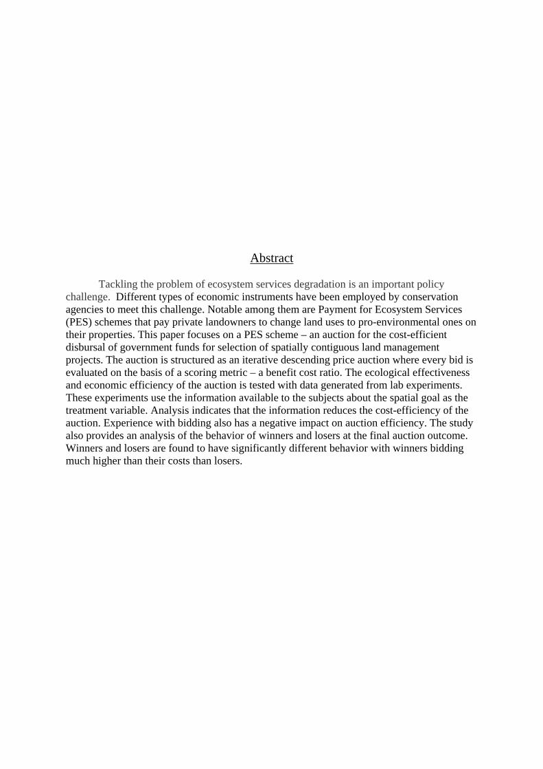
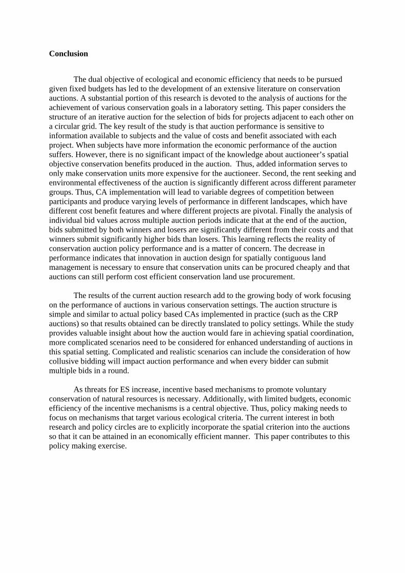
Table 4 presents the regression results for the three metrics. The value of estimates indicate that in an iterative auction with full information feedback, the significant impact of increased information content is only felt on the economic efficiency of the mechanism; the total conservation purchased is not significantly different. The signs of the estimate indicate that in the presence of information about the scoring metric, the average economic efficiency is significantly lower (at 5% level). This reduction in cost efficiency means that given the budget all purchased conservation units are more expensive in the presence of information about the spatial goal. The significant estimate (at 5%) for the dummy in the rents regression implies that when subjects know the spatial objective, they successfully exploit their combined locational and cost advantages to submit and earn higher rents (on winning). Figures 1 – 3 provide visual proofs of these results. Comparing between treatments, the value of CE is greater for all SCORE sessions except in two periods (5 and 12). Again, in Figure 2 the plot of average markups per session in SCORE sessions is greater than those in NO-SCORE. Finally no significant difference in the percentage ecological benefits is observed across treatments for multiple periods in Figure 3.

The nature of the impact of experience in the auction is captured by the Period

variable. The estimate for the log of Period is significant at 5% for the CE and at 1% in the rents and significant at 10% in the EE regression. The negative sign of the estimate in the CE and EE models indicates that with increasing experience and familiarity with the CA, the performance of the mechanism suffers. This adverse impact of experience has significance for actual policy implementation. Government run CAs are implemented multiple times during a year as well as over a period of many years. Here farmers' repeated participation in the mechanism increases familiarity and promotes learning about the structure of the scheme that can enable them to submit bids that are much higher than costs and earn high rents. A real policy based example of this phenomenon is the increase in bids submitted in CRP signups in the past (Kirwan et al. 2005). Submission of high bids over time is also represented in the current model by the positive and significant (at 1%) estimate for Log of Period in the rents regression and the positive trend in the markup graph presented in Figure 2. The inelastic nature of the impact can be attributed to the iterative format. Within a period bidding takes place in multiple rounds where successively lower bids are submitted.

So even if higher rents are earned over time, reduction in bids within a period reduces the magnitude of this experience induced rent seeking. Finally, pertinent to the current study is the impact of experience on ecological effectiveness of the mechanism. The estimate is significant at 10% and negative indicating that regardless of the quantity of information available to a group of people, with full information feedback conservation units get more expensive over time so that fewer units can be purchased with the funds available.

The log of Round is significant at 10% level of significance in the CE model and at

1% for the rents and EE models. The sign of the estimate is negative for the rents regression and positive for the other two. The sign of the estimate in the three regressions is a consequence of the iterative format under which bids submitted are decreasing over multiple rounds. In addition, the elasticity estimate in the rents regression is less than one indicating

that within a period, bidders always try to retain as much rent as possible as they reduce the value of bids submitted from one round to the other. This result is true regardless of the information content of the auction.

Dependent Variable

Economic Efficiency

Log of Rents Ecological

Effectiveness

Estimate

(Standard Error)

Random Effects

Random Effects

Random Effects Tobit

Constant .8060* (.046)

4.8873* (.230)

.5703* (.059)

Information Dummy

-.0422* (.014)

.1981** (.079)

-.0415 (.028)

Ln(Period) -.0227**

(.009) .1781* (.047)

-.0207*** (.011)

Ln(Final Round) .0380***

(.022) -.3989* (.111)

.1114* (.028)

G1 -.0179 (.019)

-.5380* (.096)

.0039 (.023)

G2 .0201 (.017)

-.7717* (.086)

.1702* (.021)

G3 -.0011 (.016)

-.5137 * (.081)

.0766* (.019)

Number of observations

141

Number of groups

12

Panel Variable

Session

*** represents significance at 10% level of significance ** represents significance at 5% level of significance *represents significance at 1% level of significance

Table 4 Regression Results for Market Performance

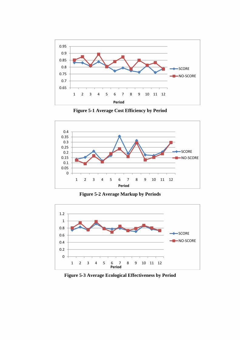
Figure 5-1 Average Cost Efficiency by Period

Figure 5-2 Average Markup by Periods

Figure 5-3 Average Ecological Effectiveness by Period

0.65

0.7

0.75

0.8

0.85

0.9

0.95

1 2 3 4 5 6 7 8 9 10 11 12

Period

SCORE

NO‐SCORE

0

0.05

0.1

0.15

0.2

0.25

0.3

0.35

0.4

1 2 3 4 5 6 7 8 9 10 11 12

Period

SCORE

NO‐SCORE

0

0.2

0.4

0.6

0.8

1

1.2

1 2 3 4 5 6 7 8 9 10 11 12Period

SCORE

NO‐SCORE

Number of

Observations Mean

Standard Deviation

Minimum Value

Maximum Value

Stable Allocation

Ecological Effectiveness

G1 36 0.757 0.09 0.55 0.92 1

G2 36 0.903 0.12 0.59 1 1

G3 36 0.8 0.08 0.58 0.94 0.84

G4 33 0.723 0.06 0.47 0.95 0.72

Economic Cost

Efficiency

G1 36 0.819 0.05 0.63 0.91 0.9

G2 36 0.844 0.07 0.68 0.94 0.78

G3 36 0.812 0.08 0.66 0.96 0.8

G4 33 0.812 0.07 0.7 1.02 0.8

Total Information

Rents

G1 36 52.12 27.56 7 160.5 35

G2 36 44.34 18.85 17.5 111 33

G3 36 59.54 15.65 33 101 35

G4 33 101.57 25.26 36 141 101

Table 5: Summary of Performance Metrics in Auction by Parameter Group

In the current research the parameter dummies represent a secondary within treatment that every subject is exposed to. For the analysis of market performance parameters are chosen on the basis of expected performance levels and pivotalness of projects in at a potential stable allocation in the auction. Table 6 provides a summary of the performance metrics by parameter regimes along with metric values for the candidate stable solution that served as the reference point for the parameter choices. Relative to the value of the metrics at the stable allocation used to choose the parameter values, their mean values attained in the auction is different. This indicates that subjects are able to exploit the private information they have and their location characteristics to earn higher rents. This higher rent seeking as mentioned makes every unit of conservation benefit dearer. In the regression, G4 is considered to be the omitted category as the total information rents that can be earned by winners at a candidate/potential stable solution is the highest under G4. In addition, the expected EE at this stable solution is the lowest as well. Now considering the results in both Tables 4 and 5, the estimates for G2 and G3 are significantly different from zero implying

that environmental performance under these regimes are significantly different from G4. The positive estimate indicates that environmental performance of the auction in these regimes is significantly higher relative to G4. One outcome of interest is that while an allocation with an EE value of 1 can be supported as the stable solution in the auction under G1 and G2, the mean EE value under G1 never reaches 1. In fact the mean EE under G1 is very near the same obtained in G4 (Table 5) which is 0.75. Thus relative to G4, there is a very high degree of rent seeking in the periods under G1 that causes the EE to plummet. This high degree of rent seeking reduces the difference in CE across parameter groups. This is seen from the mean values of the metrics in the summary Table 5 and the lack of significance for the G1, G2 and G3 estimates in the CE regression. Rent seeking also causes significant differences in performance between regimes in the rents regression as evident from the significant and positive estimates in the log of total rents regression. All the estimates are positive and significant indicating that rent seeking tendencies of all regimes are significantly different from that under G4. The negative sign of the estimates indicate that relative to G4, under all other regimes there is significantly less money left under the table. These signs and magnitudes of the parameter estimates indicate that auction performance is sensitive to parameter choices. In the context of actual policy based CA, a significant impact indicates that the performance of the CA will vary with the variation in the costs and benefits of conservation land uses and where they are located on the different working landscapes.

Analysis of Bidding Behavior in the Auction

The parameters are chosen on the basis of the properties of the stable allocation relative to . In order to statistically assess whether the behavior of winners and losers at the end of an auction period, corresponds to this theoretically stable allocation, we consider a regression with the value of average markup of bid over costs for every bidder in the final round of all the periods as the dependent variable. The markup is the differences between bids submitted and costs as a ratio of the bidders’ cost. Regression results provide insight about the variables that explain how close or far bidders’ bids are from costs when the auction ends. We expect that for a winner this markup will be higher than costs and for losers it will be lower and very near to zero or equal to it. Near zero markups also indicate high levels of competition between players. A total of 846 observations for 72 subjects are used for this analysis. The set of independent variables include the Information Dummy, the reciprocal of the period variable that represents inter-temporal learning at the individual level, the Final Round variable and the parameter dummies G1, G2 and G3. Finally a dummy is included to capture the winning or losing status of a player in any period. Let this variable be termed Winner. we use the value of the winner variable from the penultimate round to instrument for the winning status in the current period. Typically Winner would represent the status of a player in the final round of a period. However this will give rise to the problem of endogeneity. This is because bids (and hence markups) determine the winning or losing status of a player. Thus higher the bids lower the likelihood of selection. However in keeping with the theoretical properties of a stable solution, for a winner, the markup should be different from zero while for a loser the markup should be at zero. Given this problem of endogeneity, the status of a player from the past round is used as an instrument for the Winner dummy. The correlation coefficient between the Winner variable for the final round and the penultimate round in a period is approximately 0.82 justifying the use of this instrument.

Table 5 represents the set of estimated coefficients for this model. The positive and significant constant term (at 1%) indicates markups for all subjects are significantly different from zero at the end of the auction. In addition, the Information Dummy is positive and significant (at 5% level) indicating that extra information in SCORE sessions allows bidders to earn higher markups than in NO-SCORE sessions. The estimates for G1, G2 and G3 are all negative and significantly different from the constant term that picks up the effect of set G4. At the potential stable solution used to choose the values of the parameters, the total rents that winners could expect to earn was the highest under G4 relative to other regimes. Thus the negative sign of the estimates for each of G1, G2 and G3 indicate that the markups earned by players are less and they are closer to costs under these regimes. This result in turn is in keeping with the final stable solution of the auction. Of special interest to the study of markup behavior are the estimates for the Lag Winner. The positive and significant estimate for the Lag Winner variable (at 1%) indicates that winning bidders’ markups at the end of the auction are higher than losing bidders’ values. This outcome is in line with the properties of bids of winners and losers at a stable solution of the auction. However, the interaction term between Winner and the Information Dummy is not significant. Thus, the entire impact of information on markups in SCORE is captured by a level shift represented by the significant and positive dummy estimate. Having this extra information in SCORE sessions does not influence how winners demand higher markups. The estimate for Learning is negative and significant (at 5%) indicating that in latter periods, by which time, agents are familiar and have learnt to bid in the auction, markups demanded and earned are higher than in the initial periods. The trends in the average markup graphs for both SCORE and NO-SCORE in Figure 4 substantiate this claim. This result corresponds to higher and significant rent seeking in the auction in latter periods as established in the analysis of auction performance. Finally, the sign of the estimate for the Round variable is negative and significant (at 1%). This result indicates that a greater number of iterations within a period reduce markups. The analysis of final round markups presented in this section provides valuable insight about subjects’ behavior at the end of the auction. Higher markup values for winners indicate that winners’ bids are above their costs and are significantly higher than losers’ who may have bid at costs and so cannot lower bids anymore. The relative magnitude of markups across winning and losing bidders provides support for the stability properties of the theoretically stable auction allocation. Once this allocation is reached in the final round, none of the bidders have any incentive to deviate from their decisions and so the auction ends. The negative sign for the Learning variable also represents the rent seeking taking place for agents over time in these auctions.

Figure 4 Markup in Final Round

Dependent Variable : Markup over costs in Final Round of Period

Dummy .061** (0.163)

Winner 0.179* (0.018)

Learning (1/Period) -0.094** (0.038)

Final Round -0.017* (.004)

G1 -0.055***

(0.026)

G2 -0.156* (.023)

G3 -0.115* (0.022)

Constant 0.324* (0.036)

Number of Observation 846

Number of Groups 72

Unit of Observation Individual Subject

** represents estimate is significant at 5% level of significance * represents estimate is significant at 1% level of significance

Table 6: Estimates (Standard Error) for Average Markup for Final Round

0

0.05

0.1

0.15

0.2

0.25

0.3

0.35

0.4

1 2 3 4 5 6 7 8 9 10 11 12Average

 Marku

p in

 Final Round

Period

SCORE

NO‐SCORE

Conclusion

The dual objective of ecological and economic efficiency that needs to be pursued given fixed budgets has led to the development of an extensive literature on conservation auctions. A substantial portion of this research is devoted to the analysis of auctions for the achievement of various conservation goals in a laboratory setting. This paper considers the structure of an iterative auction for the selection of bids for projects adjacent to each other on a circular grid. The key result of the study is that auction performance is sensitive to information available to subjects and the value of costs and benefit associated with each project. When subjects have more information the economic performance of the auction suffers. However, there is no significant impact of the knowledge about auctioneer’s spatial objective conservation benefits produced in the auction. Thus, added information serves to only make conservation units more expensive for the auctioneer. Second, the rent seeking and environmental effectiveness of the auction is significantly different across different parameter groups. Thus, CA implementation will lead to variable degrees of competition between participants and produce varying levels of performance in different landscapes, which have different cost benefit features and where different projects are pivotal. Finally the analysis of individual bid values across multiple auction periods indicate that at the end of the auction, bids submitted by both winners and losers are significantly different from their costs and that winners submit significantly higher bids than losers. This learning reflects the reality of conservation auction policy performance and is a matter of concern. The decrease in performance indicates that innovation in auction design for spatially contiguous land management is necessary to ensure that conservation units can be procured cheaply and that auctions can still perform cost efficient conservation land use procurement.

The results of the current auction research add to the growing body of work focusing

on the performance of auctions in various conservation settings. The auction structure is simple and similar to actual policy based CAs implemented in practice (such as the CRP auctions) so that results obtained can be directly translated to policy settings. While the study provides valuable insight about how the auction would fare in achieving spatial coordination, more complicated scenarios need to be considered for enhanced understanding of auctions in this spatial setting. Complicated and realistic scenarios can include the consideration of how collusive bidding will impact auction performance and when every bidder can submit multiple bids in a round.

As threats for ES increase, incentive based mechanisms to promote voluntary

conservation of natural resources is necessary. Additionally, with limited budgets, economic efficiency of the incentive mechanisms is a central objective. Thus, policy making needs to focus on mechanisms that target various ecological criteria. The current interest in both research and policy circles are to explicitly incorporate the spatial criterion into the auctions so that it can be attained in an economically efficient manner. This paper contributes to this policy making exercise.

References

Bockstael, N. E. 1996. Modeling economics and ecology: The importance of a spatial perspective. American Journal of Agricultural Economics 78 (5): 1168.

Cason, T. N., L. Gangadharan, and C. Duke. 2003. A laboratory study of auctions for reducing non-point source pollution. Journal of Environmental Economics and Management 46 (3): 446-71.

Claassen, R., L. Hansen, M. Peters, V. Brenneman, M. Weinberg and others. Agri-Environmental Policy at the Crossroads: Guideposts on a Changing Landscape. AER 794, January 2001.

Faith, D. P. (1994). Phylogenetic pattern and the quantification of organismal biodiversity. Phil. Trans. R.Soc. Lond. B Vol. 345, pp. 45.

Fischbacher U. 2007. z-Tree: Zurich Toolbox for Readymade Economic Experiments. Experimental Economics 10: 171-178

Gilpin, M. E. in Viable Populations for Conservation (ed. Soulé, M. E.) pp. 126 (Cambridge Univ. Press, New York, 1987).

Gole, C., Burton, M., Williams, K.J., Clayton, F., Faith, D.P., White, B., Huggett, A. and Margules, C. (2005). Auction for Landscape Recovery: ID 21 Final report, September 2005. Commonwealth Market Based Instruments program, WWF Australia. Available from URL: http://www.napswq.gov.au/mbi/round1/project21.html [accessed 18 Aug 2006].

Hajkowicz, S., A. Higgins, K. Williams, D. P. Faith, and M. Burton. 2007. Optimisation and the selection of conservation contracts*. Australian Journal of Agricultural and Resource Economics 51 (1): 39-56.

Kirwan, B., R. N. Lubowski, and M. J. Roberts. 2005. How cost-effective are land retirement auctions? estimating the difference between payments and willingness to accept in the conservation reserve program. American Journal of Agricultural Economics 87 (5): 1239.

McAfee, R. P., and J. McMillan. 1996. Analyzing the airwaves auction. Journal of Economic Perspectives 10(1): 159-175.

Plott, C. R. 1997. Laboratory experimental testbeds: Application to the PCS auction. Journal of Economics & Management Strategy 6 (3): 605-38.

Reeson AF, Rodriguez L, Whitten SM, Williams KJ, Nolles K, Windle J, Rolfe J. Applying competitive tenders for the provision of ecosystem services at the landscape scale: Paper. Applying Competitive Tenders for the Provision of Ecosystem Services at the Landscape Scale. Paper accepted for BIOECON conference, Cambridge, September 2008.

Rolfe, J., and J. Windle. 2006. Using field experiments to explore the use of multiple bidding rounds in conservation auctions. Canadian Journal of Agricultural Economics.

Rolfe, J., J. Windle, and J. McCosker. 2009. Testing and implementing the use of multiple bidding rounds in conservation auctions: A case study application. Canadian Journal of Agricultural Economics/Revue Canadienne d'Agroeconomie 57 (3): 287-303.

Vane-Wright, R. I., C. J. Humphries, and P. H. Williams. 1991. What to protect?--systematics and the agony of choice. Biological Conservation 55 (3): 235-54.