An Invitation Control Policy for Proactive ServiceSystems: Balancing Efficiency, Value and Service

Level

Galit B. Yom-Tov, Liron Yedidsion, Yueming Xiegality@technion.ac.il, lirony@ie.technion.ac.il, yueming.xie@hotmail.com,

Technion—Israel Institute of Technology

Problem definition: We study the problem of designing a dynamic invitation policy for proactive ser-

vice systems with finite customer patience under scarce capacity. In such systems, prior knowledge regarding

customer value or importance is used to decide whether the company should offer service or not.

Academic / Practical Relevance: Proactive service systems are becoming more popular, as data avail-

ability and machine-learning techniques are developed to forecast customer needs. However, very little is

known on the efficient use of such tools to promote and manage service systems.

Methodology: We use fluid approximation and the Filippov convex method to analyze system dynamics

and develop approximations for important performance measures.

Results: We show that while prioritizing customers in descending order of their rµ ranking (as long as

there are idle servers in the system) is optimal on the fluid level, refinements are necessary in the presence

of abandonment on the stochastic level. We propose an rµ−N policy to account for customer patience.

Managerial Implications: Our policy can be used to promote service effectiveness, and allow decision

makers the means to trade off service level against costs in such systems explicitly. Using a case study of a

transportation service provider we show that such a policy can triple revenue compared to random arrivals

(non-proactive policy).

1. Introduction

Classic service models mostly consider cases in which the customers autonomously seek service

from companies. Thus, the arrival rate is highly variable and exogenous to the system. Decision

makers then make strategic decisions on how to cope with a stream of arrivals, regard service level

and decide whether to serve all customers and what resource to assign. In contrast, new technology

allows companies to impact arrivals by reaching out to potential customers. We refer to service

systems that implement such a technology as proactive service systems. A prerequisite is obtain-

ing historical information on potential customers. The companies use such information to classify

potential customers, assess their current value, and invite them to the system for personalized

assistance. In this type of system, the company needs sound information indicating that the poten-

tial customer is likely to require or benefit from service. Then, during service, the company might

expose the agents to the profile and data of the current customers, which may help them promote

1

2

revenue as well as improve customer experience. Proactive service systems are becoming more and

more common. We provide here two examples—the first of online (retail support) services, and the

second from the healthcare domain.

The service industry is undergoing a digital revolution. Services have become more and more

automatic and easy to use, and service companies have become more accessible through new

service channels and social media (e.g., Twitter or Facebook), corporate websites, or messaging

applications (e.g., WeChat and WhatsApp). Providing service through digital interfaces offers new

opportunities to explore service systems that were not possible in the past (Rafaeli et al. 2017,

Yom-Tov et al. 2018). Many companies use web-based channels to support or complement self-

services. Such a combination is beneficial both to companies and customers, as self-services have

the benefit of flexible timing, visualization and low cost, while a personal connection through other

service channels is sometimes needed to solve more complicated problems or to enhance customer

experience. These days, many companies adopt an online customer service chat (CSC) system as an

attractive complement for the online self-services, for its economy and immediacy. Hence, it is not

surprising that CSC systems also started to get attention from the queueing research community.

For example, Luo and Zhang (2013), Tezcan and Zhang (2014), Cui and Tezcan (2016) and Legros

and Jouini (2019) studied the staffing and how to balance multi-tasking between agents in CSCs.

Like regular call-centers, a CSC can be initiated by the customer using a ‘contact us’ button;

CSC systems also enable companies to initiate the service by extending an invitation for a chat on

the customer’s screen. We concentrate on the latter option. In order to decide to which customers to

offer service, the company collects the customers’ browsing behavior on their website and additional

historical data. Then, the company evaluates that consumer’s ‘service value’. The high-value visitors

may then be invited to the chat based on the current agent availability. Customers accepting the

invitation enter a queue, after which they are connected to an available service agent. Figure 1

presents an example of customer value distribution of a transportation company, provided by the

LivePerson Inc. This distribution fits nicely to a mixture of four customer classes. The scores here

were created using the customer activity on the website, and are correlated with the revenue the

firm is expecting to gain if service is provided to that particular customer. Using such information

and selecting who to serve wisely can increase the brand revenue significantly. We will use this

data for the case study in §8 where we implement the policies developed in this paper, discussing

some implementation challenges and demonstrating its value.

Our second example is a proactive healthcare system in which patients are invited for a periodic or

a follow-up medical examination, such as after surgery (Shadmi et al. 2015, 2017). Such preventive

care policies aim to identify health problems before they become severe and reduce readmissions

and mortality by prompt intervention. Screening all people is wasteful and not possible due to

3

0.00.10.20.30.40.50.60.70.80.91.01.11.21.31.4

7 257 507 757 1007 1257 1507 1757

Rela

tive

freq

uenc

ies %

Customer score (resolution 5)

OnlineChatsV2; January-February 2016; All daysFitting Mixtures of Distributions

Empirical Total Gamma Gamma Gamma Gamma

Figure 1 Customer value score distribution

capacity constraints. Therefore, the decision makers invite only an appropriate number of high-risk

patients for preventive care. This will potentially both reduce the cost of further treatment, and

improve health (Shadmi et al. 2015, 2017). However, even though the methodologies for evaluating

which patient is more likely to need such services are improving, operational and economical

considerations limit the implementation of such preventive care policies. One such limiting factor

is the number of nurses and physicians who can do that checkup. A certain capacity should be

kept available, at all times, for the regular patients who come with unexpected health issues. The

challenge is to balance the two groups properly and plan the invited patients in a manner that will

not overload the system, but will take into account their medical risk properly.

The organizations we described need to decide how many customers to invite and when. This is

the operational question we strive to answer. Too many invited customers will lower the service level

(increase waiting and abandonment) and therefore increase cost. Moreover, from the customer point

of view, receiving an invitation and then a poor service level, can cause anger and frustration—the

company may be better off not inviting them in the first place. On the other hand, a low invitation

rate is also undesirable since the company may miss valuable customers while having idle agents.

Hence, invitation strategies need to balance customer value, costs and service levels.

1.1. Literature Review

1.1.1. Admission Control. An invitation problem can be thought of as a special type of

an admission control problem, because it can be interpreted as whether to accept or reject each

potential arrival, while not incurring any penalty for rejection (except of lost revenue). There

are many papers that discuss admission control problems; we focus on those that consider also

service levels (e.g., waiting and abandonment). Koole and Pot (2011), motivated by an inbound

call center, discussed an admission control problem that maximizes profit of an M/M/s/n+M

4

queueing system by controlling its trunk and agent number. Later on, Ward and Kumar (2008)

considered general distributions of arrival and service rates in a conventional heavy-traffic regime.

Kocaga and Ward (2010) tried to minimize the infinite horizon expected average cost associated

with customer blocking, abandonments and server idleness of the Erlang-A queueing system. They

used the Markov decision process (MDP) and the diffusion control problem (DCP) in the Quality

and Efficiency-Driven (QED) regime, to obtain an asymptotically optimal policy. Weerasinghe

and Mandelbaum (2013) considered the G/M/n/B +GI queueing system for the finite horizon

cost minimization under a QED regime. They developed a static control policy in the form of a

constraint on the system capacity. All the above papers assume homogeneous customers while we

assume multiple classes of customers with different value, cost, patience, and service requirements.

The most recent paper to study admission control problems from a revenue maximization per-

spective was Sanders et al. (2017). They suggested that a threshold policy is asymptotically optimal

in the QED regime, for certain cost function structures. Early work on the admission control prob-

lem with heterogeneous customers can be found in Miller (1969), where an optimal static threshold

policy for a multi-server loss system was explored. Yoon and Lewis (2004) extended this research

to provide a non-stationary policy. Nevertheless, all the above ignore abandonments, which we

show to have an important role when deciding on threshold values. Zayas-Caban and Lewis (2017)

studied the impact of customers’ patience on such admission (and routing) policies, analyzing a

two-class two-server type loss system, in which abandonment happens both during queueing and

service. Using MDP analysis, they showed that no simple structured policy exists for all parameter

combinations, which justifies using approximations as our approach.

A different way to control arrival rate in revenue maximization problems is to use pricing. For

example, Kumar and Randhawa (2010), Maglaras et al. (2018) consider pricing mechanisms under

capacity constraints and service differentiation. In the service setting discussed here, we assume

that customer value is given, and one cannot influence a customer’s decision by changing prices.

Instead, we influence total revenue by applying a selective invitation control policy. Another way

to influence revenue is through advertising that may impact demand rate. For example, Olsen

and Parker (2008) and Sethi and Zhang (1995) studied advertising in the context of inventory

management, and Afeche et al. (2017) considered it for service systems. The latter use three types

of control variables: advertising expenses, number of servers, and service allocation among different

customer types (as elaborated upon in the next subsection).

1.1.2. A Multi-class Customer Routing. Customer ranking is an essential feature of proac-

tive service systems, thus yielding a multi-class customer setting. This raises the question of what

routing policy the servers should use when prioritizing customers waiting in queue. We only review

5

here papers that consider a setting with abandonments. Atar et al. (2004, 2010, 2013) suggested the

cµ/θ rule for multi-class multi-server systems with impatient customers. They showed that such

a routing policy asymptotically attains the lower bound in both preemptive and non-preemptive

cases. This policy was generalized to account for general patience and service distributions by Bas-

samboo and Randhawa (2016). The cµ/θ policy aims to decrease costs, while we strive to maximize

revenue. Routing policies were studiesd in the above-mentioned paper of Zayas-Caban and Lewis

(2017) as well as in Jacobson et al. (2012). The latter showed that when the number of customers

is known (for example in the case of evacuating patients from a mass-casualty event), and patience

is generally distributed, the optimal priority schema depends on the parameter combination, and

in many cases takes the form of an rµ policy. A similar policy was also suggested by Afeche et al.

(2017) to maximize long-term, life cycle revenue in a customer network in which customers impact

one another via word-of-mouth. Therefore, we assume in our model that once customers have

entered the system the agent prioritizes them according to an rµ policy.

We also show that the rµ policy is near-optimal for invitation control (via fluid approximation),

which can be applied via a simple threshold policy. However, in many systems, it was found that

control policies based on regular fluid approximations may be too crude, and suggest an atrophied

threshold. This was the case for the X model studied by Perry and Whitt (2011), wherein they

considered a two-class system, in an overloaded X system, with a threshold-based routing policy.

Their routing depended on queue length in each queue. The analysis was focused on a special type

of fluid approximation, which has a non-smooth structure resulting from that threshold policy. A

similar methodology and structure was used by Chan et al. (2014), Yom-Tov and Chan (2018) for

other queueing models, utilizing the Filippov (Filippov 1988) analysis to study the dynamics of

the fluid flow. In this research, we use a similar technique to extend our analysis to more refined

threshold policies and approximations.

This paper continues as follows: In §2, we formally define our model. In §3, we use LP to solve the

fluid model for our multi-server system with impatient heterogeneous customers and determine an

optimal invitation policy. We refine the fluid approximation model in §5 using the Filippov method

and analyze its equalibria. The Filippov approximation allows for various threshold controls. In §6,

we develop approximations for both revenue evaluation and service level indicators. All the acquired

approximations perform well. In §7 we discuss several extensions for our model. Specifically, the

case in which customers delay their decision as to whether to accept the invitation (§7.1) and the

case of time-varying arrival rate (§7.2). Finally, in §8 we demonstrate via a case study that our

approach works well in reality too; we compare it to a non-proactive policy in which customers are

all invited, and to a different proactive policy that is currently applied by the company.

6

2. Model Description

The model we consider is a multi-class, multi-server queueing service system (Figure 2), with m

homogeneous servers. Each customer class has unique characteristics that define their behavior

and value. The number of classes is denoted by k. The stream of potential customers of Class

i are realized according to a Poisson process with rate λi, where i ∈ K = 1, ..., k. Following a

predetermined invitation policy, the system invites Class i customers to join the system with

rate λi ≤ λi. We assume that all invited customers accept that invitation instantaneously. (This

assumption will be relaxed in §7.1.) Customers wait in a class dedicated queue with infinite capacity

until they are assigned to a server. During waiting, customers may abandon the queue due to

their lack of patience. We assume that customer patience of Class i customers is Exponentially

distributed with rate θi. Each customer requires an Exponentially distributed service time with

mean 1/µi (depending on the class). Every service provided to Class i’s customer brings a reward

with a value of ri. However, waiting time and abandonment are penalized with positive cost chi per

unit of waiting time and cabi per renege customer, respectively. Aiming to maximize revenue—the

difference between system reward and cost—a dynamic control policy was developed to determine

the effective invitation rates.

𝑍𝑍1

Potential arrival rate 𝝀𝝀𝟏𝟏

𝜽𝜽𝟏𝟏

Leave

Invitation rate 𝝀𝝀𝟏𝟏

𝝁𝝁𝟏𝟏

𝑍𝑍2

Potential arrival rate 𝝀𝝀𝟐𝟐

𝜽𝜽𝟐𝟐

Invitation rate 𝝀𝝀𝟐𝟐

𝝁𝝁𝟐𝟐

𝑍𝑍𝑘𝑘

Potential arrival rate 𝝀𝝀𝒌𝒌

𝜽𝜽𝒌𝒌

Invitation rate 𝝀𝝀𝒌𝒌

𝝁𝝁𝒌𝒌

…

Figure 2 System structure

We let Qi(t) and Zi(t) be the number of customers of Class i in queue and in service at time t,

respectively. We denote by

Xi(t) :=Qi(t) +Zi(t) (1)

(where := stands for equality in definition) the corresponding total number of Class i customers in

the system. All servers share the same server pool with a total of m statistically identical servers

who cater to all types of customers. Therefore,

k∑i=1

Zi (t)≤m. (2)

7

Denote Ai as the arrival processes with rate λi, and Di and Ri, as the departure processes

from service and abandonment, respectively. We denote the initial condition of the system by

X(0) = (X1(0), ...,Xk(0)). The system dynamics clearly satisfy the following relation (for each class

of customers)

Xi (t) =Xi (0) +Ai (t)−Di (t)−Ri (t) , i∈K. (3)

Any proposed invitation policy has to satisfy the dynamics provided by Eqs. (1)–(3). A control

policy may be defined as a rule for inviting customers to service, with Ai(t) understood to be the

control variable.

By using the system state variables, the instantaneous cost of a Class i customer at time t,

Ci (t)dt, can be computed by

Ci (t)dt= chiQi (t)dt+ cabi dRi (t) .

Because the patience of any class of customer is Exponentially distributed with rate θi, at time t,

the expected abandonment rate of a Class i customer can be written as θiQi (t) (Atar et al. 2010).

For computational simplicity, ci = chi + cabi θi is used as a positive unified cost parameter of Class i

from now on. Hence, the above cost function can be modified to:

Ci (t) = chiQi (t) + cabi (θiQi (t)) = ciQi (t) .

Meanwhile, the system is rewarded by each customer whose service is completed. Because the

service process is Exponentially distributed with rate µi, the customer service completion rate is

dDi (t) = µiZi (t) .

Thus, the total instantaneous system revenue, V, is the summation of the revenue of all classes,

that can be expressed by

V (t) =∑i∈K

(riµiZi (t)− ciQi (t)).

Furthermore, by considering the problem over an infinite time horizon, our objective is to find an

invitation policy satisfying the system dynamics and constraints (defined by Eqs. (1)–(3)) that

achieves the maximum average revenue defined by

Eπ [V ] = limT→∞

1

TE∫ T

0

(∑i∈K

(riµiZi (t)− ciQi (t))

)dt. (4)

Next, we optimize a fluid scale version of this stochastic model to acquire some understanding

of the invitation policy structure.

8

3. The Fluid Policy

In this section, we consider a steady-state fluid model and the corresponding linear program (LP)

that are suggested according to the stochastic model of the previous section. We provide the

solution of this fluid LP that suggests the basic rµ policy, which is the foundation we build upon

for further developments.

Denote xi, qi and zi as the long-run fluid averages of the process Xi (t), Qi (t) and Zi (t) for Class

i customers, i∈K. These fluid functions satisfy, in steady state, the following set of equations

xi = qi + zi ∀i∈K,

λi = µizi + θiqi ∀i∈K,

λi ≤ λi ∀i∈K,∑i∈K

zi ≤m,

xi, zi, qi ≥ 0 ∀i∈K.

Under the above constraints, our objective is to maximize the total revenue over all sets(λi, xi, qi, zi

). This optimization problem corresponds, after simplification, to the following linear

program (LP) problem

max∀zi,qi

∑i∈K

(riµizi− ciqi) (5)

s.t.∑i∈K

zi ≤m

µizi + θiqi ≤ λi, ∀i∈K

zi, qi ≥ 0, ∀i∈K.

Since the above LP includes several inequality constraints, we use the Karush–Kuhn–Tucker (KKT)

conditions (Karush 1939, Kuhn and Tucker 1951) to determine the necessary optimality conditions

of this convex problem. The Lagrangian is

L (zi, qi, α,βi, γi, σi) =−∑i∈K

(riµizi− ciqi) +α

(∑i∈K

zi−m

)+∑i∈K

βi (µizi + θiqi−λi)−∑i∈K

γizi−∑i∈K

σiqi.

The KKT conditions for each Class i are

− riµi +α+βiµi− γi = 0, ci +βiθi−σi = 0, α

(∑i∈K

zi−m

)= 0, (6)

βi (µizi + θiqi−λi) = 0, γizi = 0, σiqi = 0,

α,βi, γi, σi ≥ 0.

9

Since ci is positive, and βi, θi are non-negative, all σi must be positive to satisfy the second

condition of Eq. (6). Therefore, according to the sixth condition, any qi must equal 0. Because the

KKT conditions are necessary, the above result means that the optimal fluid invitation policy does

not permit accumulation of queues for any class of customers.

By substituting qi = 0 into the original LP in Eq. (5), the problem is simplified into

max∀zi

∑i∈K

(riµi)zi

s.t.∑i∈K

zi ≤m

zi ≤ λi/µi,∀i∈K

zi ≥ 0,∀i∈K.

Without loss of generality, we can re-label the classes according to a decreasing order of their rank,

defined by the product riµi, i.e.:

r1µ1 ≥ r2µ2 ≥ . . .≥ rkµk.

Obviously, the optimal solution is to assign all the available servers to serve customers in decreasing

order of their Class i until all servers are occupied, i.e., as long as there are at least λi/µi servers

available, Class i customers will be fully invited. Denote k0 as the last class that invites all its

potential customers. The optimal solution for LP (5) is

z∗ =

(λ1

µ1

,λ2

µ2

, . . . ,λk0

µk0

,m−k0∑i=1

λiµi,0, . . . ,0

). (7)

q∗ = (0,0, . . . ,0) .

In other words, in the fluid scale, the optimal invitation policy is: rank customer classes by riµi,

then use all system service capacity to invite customers from the highest rank possible, until the

system runs in the critically-loaded regime, for which∑zi =m. Therefore, Class i (i∈ 1, ..., ko)

customers shall be invited in rate λi = λi, and Class k0 + 1 customers shall be invited in rate

λk0+1 =

(m−

k0∑i=1

λiµi

)µk0+1. This results in three customer groups: all invited, partially invited and

non-invited. We call this the rµ-policy.

Note that this policy ignores both waiting cost and customer patience. This is very intuitive as

this policy enables no costs of waiting and abandonment with fully occupied servers which runs

in a maximal combination of income. This heavily depends on the fluid scale which assumes that

for every lost customer, there is an immediate replacement with the same revenue. When one

tries to implement such a policy to finite-size stochastic systems, this disregard of waiting and

abandonment will be problematic. We demonstrate that in the next section.

10

We also note that since the optimal solution to the fluid relaxation problem (5) will have qi = 0

for all i, then consequentially, that solution is necessarily an upper bound for the original stochastic

optimization problem of maximizing V in Eq. (4). However, the fluid relaxation is not realistic

since the stochastic process will never have exactly zero queue and full utilization at all times.

Therefore, this is a theoretical bound. How close we get there depends on how we apply the fluid

policy which is the focus of our next section.

4. Applying the rµ Invitation Policy: Effectiveness and Limitations

The fluid policy suggests an optimal rµ-policy. As the fluid model ignores the inherent stochastic

nature of the system, the simplest implementation suggested by the fluid model is a static pol-

icy in which customers are invited at a constant rate, according to their class. This is achieved

by randomly inviting potential customers of the partially invited class, k0 + 1, with probability

λk0+1/λk0+1. We refer to this implementation option as randomized invitation. In this implemen-

tation, the stochastic characteristics of the arrival process remain the same, and is easy to ana-

lyze. However, in practice, this policy could be improved. The rµ policy drives the system to

be critically-loaded. A critically-loaded system has a non-negligible chance of being both over-

loaded and underloaded. Accordingly, the rµ policy could benefit from a dynamic approach which

introduces a threshold so as to invite any arriving low class customer as long as the system is

underloaded (below the threshold) and not invite any low class customer when it is overloaded

(above the threshold). This will result in overloaded periods in which the arrival rate of Class k0 + 1

is 0 and complementary underloaded periods in which the arrival rate is the original maximal rate,

λk0+1. The threshold, that determines when we switch between those two operational modes, refers

to the total number of customers in the system, either being served or waiting in queue. We refer

to this policy as an rµ−N policy. The fluid analysis suggests setting the threshold to m. As we

explained, this is because on the fluid scale customers appear instantaneously and the system is

perfectly balanced. However, in practice, there will be periods with an accumulated queue or idle-

ness. Therefore, customers’ attributes such as patience directly affect our objective function and

need to be taken into consideration. Intuitively, as rk0+1µk0+1 increases, the loss caused by idleness

increases, which should drive us to overload the system and increase the threshold. On the other

hand, as θk0+1 and ck0+1 increase, the loss caused by overloading increases, which should drive us

to decrease the probability of queue accumulation and thus, decrease the threshold. Note that N

could be any positive number, which means that the control may be either on the queue length

(N ≥m) or on server idleness (N <m).

To exemplify this intuition, we simulated a two-class system with 40 servers. Class 2 have lower

rank and are partially invited. The class of high ranked customers has λ1 = 30, µ1 = 1, r1 = 15,

11

θ1 = 0.5, cab1 = 10 and ch1 = 1. For the class of low ranked customers we simulate three sets of

parameters. All three sets share the same arrival rate, service rate, and penalties: λ2 = 20, µ2 = 0.8,

cab1 = 5 and ch1 = 1. However, the sets differ in their relative reward and patience according to the

following cases:

Case 1: r2 = 13 and θ2 = 0.4 — high reward, high patience;

Case 2: r2 = 13 and θ2 = 0.8 — high reward, low patience;

Case 3: r2 = 10 and θ2 = 0.4 — low reward, high patience.

For each one of the cases, we ran a simulation with different threshold values, N , calculating the

expected total revenue (after system stabilization). Figure 3 shows how the optimal threshold may

divert from m according to the different parameters, and fits in general our intuition above. The

graph also indicates by horizontal dashed lines the revenue achieved via implementation of the

randomized invitation policy, and with dotted lines the theoretical upper bound (the LP solution).

(Note that the upper bounds for cases 1 and 2 coincide.) We observed a significant difference in

which the rµ−N policy outperforms the randomized policy in all scenarios if N is chosen wisely.

Note that the differences between different thresholds are not large, meaning that the fluid policy

is around the right value, but improvement can be done. This motivates us to improve our analysis

and look for a more refined policy than the fluid one. Nevertheless, from a practical perspective

keeping the structure of that policy is important, because we would like it to be implementable in

large-scale systems which requires a minimum amount of information.

Figure 3 Revenue as a function of thresholds for different parameters

5. Analyzing System Dynamics with Threshold Policy

From the previous sections, we learned that in order to use a proactive invitation policy correctly,

we need to take extra measures to prevent both overloading the system with low priority customers

12

and underloading the system by creating unnecessary idleness. In addition, we learned in §3 that

the control threshold shall restrict the partially-invited customer class, assuming that higher classes

will always be invited and lower classes will never be invited. Therefore, this reduces the analysis

to a 2-class invitation policy in which the system has enough capacity to serve all Class 1, high

priority customers, but does not have enough capacity to serve the entire customer population, as

stated formally in Assumption 1. The simplified 2-class system is presented in Figure 4.

Assumption 1. The number of servers in the system, m, is such that λ1/µ1 ≤m ≤ λ1/µ1 +

λ2/µ2.

m

Class 1

rate λ1

Abandon

rate θ1

m Servers

Allow preemption

Service rate μ1 / 2

Class 2

rate λ2N

Not invited

Invited

Abandon

rate θ2

Figure 4 The simplified two-class model of threshold policy

Remark 1. One can easily reduce the multi-class system—distinguished here by a ’ on all its

parameters, λ′ and µ′—to a 2-class system by summing the arrival rates of the all-invited classes

such that the total arrival rate of Class 1 is λ1 =∑k0

j=1 λ′j and λ2 = λ′k0+1; service rates will be

averaged by µ1 =(∑k0

j=1 λ′j

)/(∑k0

j=1

(λ′j/µ

′j

)), and µ2 = µ′k0+1.

Without loss of generality, we assume that Class 1 customers have a higher ranking, i.e., r1µ1 >

r2µ2. A predetermined threshold N controls the admission of Class 2 customers. Namely, the

system admits lower ranking customers only if the total number of customers in the system is lower

than the threshold. Note that the original fluid policy optimization suggested that N = m (no

queues). After entering the system, if all servers are busy, the customers wait in a priority queue

in accordance with their rank. For tractability reasons, we assume that preemption is permitted.

The effect of preemption on the performance measures in similar multi-server systems was shown

to become negligible as systems become larger (Atar et al. 2010).

In this section, we analyze the effect of the threshold value on different performance metrics.

The first is equilibrium analysis to determine the expected number of customers of Class i in the

system, xi. This will be used to estimate the effective arrival rate, which is a function of the fraction

of time in which customers are invited P (x1 +x2 <N). The dynamics of this model is captured by

the following differential equations:

x1(t) = λ1−µ1z1(t)− θ1q1(t)

13

x2(t) = Ix1(t)+x2(t)<Nλ2−µ2z2(t)− θ2q2(t)

q1(t) = x1(t)− z1(t) (8)

q2(t) = x2(t)− z2(t)

z1(t) = x1(t)∧m

z2(t) = x2(t)∧ (m−x1(t))+

where Ix is an indicator representing whether condition x is true (1) or false (0), the symbol ∧ is

the minimal operator and (·)+ is max0, ·. Those equations can be simplified into:

x1 (t) = λ1−µ1 (x1 (t)∧m)− θ1(x1 (t)−m)+

(9)

x2 (t) = I(x1(t)+x2(t))<Nλ2−µ2

(x2 (t)∧ (m−x1 (t))

+)− θ2

(x2 (t)− (m−x1 (t))

+)+

.

The above dynamics (9) (of the general form x= f(x)) has a discontinuous right-hand side. The

discontinuity happens when x1 +x2 =N . Our goal is to examine the long-term behavior of the fluid

system, i.e., the behavior as t→∞ and determine the steady state denoted x(t) := [x1(t), x2(t)],

and x = (x1, x2) as the long-term value, such that x = limt→∞ [x1(t), x2(t)|x(0) = x0].

Analyzing the long-term behavior, we aim to determine if such a limit exists, is finite and/or

depends on the initial condition, x0. Several definitions are needed. Consider a dynamic system

that is represented by x = f(x). We denote by Φ(x0, t) the flow at time t, given initial condition

x0. Then, the flow dynamics over time are defined at time t by ddt

Φ(x0, t) = f (Φ(x0, t),Φ(x0,0)) =

x0. Bernardo et al. (2008) defined the equilibrium state (or point), stability (and instability),

asymptotically stable and globally asymptotically stable as:

Definition 1 (Equilibrium). A state x is an equilibrium state (or equilibrium point) of the

ODE x= f(x) if Φ(x, t) = Φ(x,0) for all t.

Denote in state-space ball BR = x| ‖x‖<R, and sphere SR = x| ‖x‖=R.Definition 2 ((Lyapunov) Locally Stable Equilibrium). The equilibrium state, x, is

said to be (Lyapunov) locally stable if for any R > 0, there exists an r > 0 such that if ‖x‖< r,

then ‖Φ(x, t)‖<R for all t≥ 0. Otherwise, the equilibrium point is unstable.

Definition 3 (Asymptotically Stable Equilibrium). The equilibrium point x is asymp-

totically stable if it is stable, and if in addition there exists r > 0, such that ‖x‖< r implies that

Φ(x, t)→ x as t→∞.

Definition 4 (Globally Stable Equilibrium). If asymptotic stability holds for any initial

states, the equilibrium point is said to be globally asymptotically stable.

As a baseline, we start the analysis with two extreme cases: a system that invites only high

ranked customers, N = 0, and a system that invites all low ranked customers, i.e., no control policy,

N =∞.

14

5.1. Invite Only Class 1 Customers (rµ-0 policy)

When the system stops inviting low value customers (N = 0), system dynamics are simplified to

the following continuous form:

x1(t) = λ1−µ1 (x1 (t)∧m)− θ1(x1 (t)−m)+

(10)

x2(t) =−µ2

(x2 (t)∧ (m−x1 (t))

+)− θ2

(x2 (t)− (m−x1 (t))

+)+

.

Due to abandonment, this system is always stable and converges to its equilibrium, denoted as

xL = (xL1 , xL2 ). Note that since there are no invitations of Class 2 customers, x2(t)< 0,∀t, and after

some finite time ε, x2 becomes 0 and from that time on, the system behaves like an Erlang-A

queue. Hence, the number of Class 1 customers in equilibrium is λ1/µ1.

Theorem 1. In system (10), under Assumption 1, the following equilibrium is globally asymp-

totically stable, i.e., the system fluid converges to:

xL =

(λ1µ1

0

)(11)

The proof of this result is provided in Appendix A. It is based on standard Lyaponov techniques.

5.2. Always Invite Both Customer Classes (rµ-∞ policy)

When the system never selects a specific customer class to invite, but instead always invites both

classes, no admission control is implemented (N =∞). In this situation, the dynamics can be

simplified into

x1(t) = λ1−µ1 (x1(t)∧m)− θ1 (x1(t)−m)+

(12)

x2(t) = λ2−µ2

(x2(t)∧ (m−x1(t))

+)− θ2

(x2(t)− (m−x1(t))

+)+

.

In this case, standard Lyaponov techniques would not work as the trajectories are not monotone.

This is demonstrated in Figure 5, where we simulated several trajectories of the system. Each

trajectory starts with some random initial point. Note that the trajectory marked with ‘*’ demon-

strates that x2 is not monotonic. It first increases for a while and then decreases to the equilibrium.

Still we find that all trajectories converge to the same equilibrium (their intersection point), as

stated by the following theorem.

Theorem 2. Under Assumption 1, the fluid (12) converges to the following globally asymptoti-

cally stable equilibrium:

xH =

(λ1µ1

λ2−(µ2−θ2)(m−λ1/µ1)

θ2

). (13)

15

0 5 10 15 20 25 30 35 40x

1

0

10

20

30

40

50

60

x 2

Figure 5 Trajectories of system without admission control

The proof of this result can be found in Appendix B. We would like to provide intuition to

the equilibrium. The high priority class, Class 1, sees an underloaded Erlang-A queue, with an

equilibrium of xH1 = λ1/µ1, and Class 2 sees an overloaded Erlang-A queue with m−λ1/µ1 servers;

therefore, for Class 2 customers, the equilibrium is xH2 = (λ2− (µ2− θ2) (m−λ1/µ1))/θ2. Moreover,

by comparing Theorem 2 to Theorem 1, we note that xL1 = xH1 , meaning that the high priority

class is not affected by whether the low priority class is invited or not.

The situation when not all customers are invited is not that simple, and is the topic of our next

section.

5.3. Applying Threshold Policy

We now go back to analyzing the long-term dynamics of the fluid model presented in the beginning

of this section in Eq. (9). The main challenge is the discontinuity at x1 + x2 = N . To overcome

that switching boundary in which the system changes its behavior from inviting to stop-inviting

customers, we use the Filippov convex method (Filippov 1988, Bernardo et al. 2008). The basic

premise is to divide the state space into regions where the ODE is smooth and continuous in order to

leverage existing results of smooth dynamical systems. A separate region—the switching boundary

region, Σ—is defined as the states of discontinuity in the ODE. The approach is to transform

the differential equation into a differential inclusion, where the differential function is now a set-

valued function. Additionally, Filippov (1988) proves that solutions to the original discontinuous

differential equation coincide with solutions to the appropriately defined differential inclusion.

In what follows, we will discuss first how to transform Eq. (9) into the appropriate differential

inclusion. Then, we will state the main theorem of the paper (proof appears in Appendix C).

To start, we separate the state space, R2+ into two regions, R1 and R2, and the switching

boundary, Σ, between them as follows:

R1 , (x1, x2) |x1 +x2−N > 0 , R2 , (x1, x2) |x1 +x2−N < 0 ,

16

Σ, x : x1 +x2−N = 0 .

In the regions R1 and R2, the ODE is smooth. However, the ODE is discontinuous at the switching

boundary Σ. The Filippov methodology overcomes this by transforming the differential equation

into a differential inclusion by using a convex combination of the smooth flows defined in R1 and

R2 on the switching boundary, Σ. We define the fluid function fi(x), x ∈Ri, as the smooth ODE

in these regions:

f1(x) =

(λ1−µ1 (x1 ∧m)− θ1(x1−m)

+,

−µ2

(x2 ∧ (m−x1)

+)− θ2

(x2− (m−x1)

+)+

)

f2(x) =

(λ1−µ1 (x1 ∧m)− θ1(x1−m)

+,

λ2−µ2

(x2 ∧ (m−x1)

+)− θ2

(x2− (m−x1)

+)+

).

(14)

Note that f1(x) and f2(x) are exactly the system analyzed in §5.1 and §5.2, respectively.

Now, our ODE (9)—x = f(x)—can be represented via a Filippov ODE (a.k.a. a differential

inclusion):

x∈F(x) =

f1(x), if x∈R1,ϕf1(x) + (1−ϕ) f2(x)|0≤ϕ≤ 1, if x∈Σ,f2(x), if x∈R2,

(15)

which we write explicitly for x∈Σ as,

x1 = λ1−µ1 (x1 ∧m)− θ1 (x1−m)+,

x2 = (1−ϕ)λ2−µ2

(x2 ∧ (m−x1)

+)− θ2

(x2− (m−x1)

+)+

, ϕ∈ [0,1] .

By using xH = (xH1 , xH2 ) and xL = (xL1 , x

L2 ) that are defined in Theorems 1 and 2, respectively,

the equilibrium of system (15) is stated in the following theorem.

Theorem 3. Under Assumption 1, the system (15) converges to the following globally asymp-

totically stable equilibrium:

x =

xL, if N ≤ xL1 +xL2 ;xG, if xL1 +xL2 <N <xH1 +xH2 ;xH , if xH1 +xH2 ≤N,

(16)

where

xG =

(λ1µ1

λ2(1−α)−(µ2−θ2)(m−λ1/µ1)

θ2

), (17)

and

1−α=

µ2

(m−λ1

µ1

)+θ2(N−m)

λ2, if m<N ;

µ2

(N−λ1

µ1

)λ2

, if N ≤m.(18)

The assumption that, xL1 + xL2 ≤ xH1 + xH2 , results from xL2 = 0 and xH1 = xL1 .

Furthermore, by using Theorem 3 and the results of Bernardo et al. (2008), on the differential

inclusion, we obtain the following:

17

Corollary 1. Under Assumption 1, the proportion of time inviting low priority (Class 2) cus-

tomers in the system defined by Eq. (15) is given by:

limT→∞

1

T

∫ T

0

Ix1(t)+x2(t)<Ndt=

0, if N ≤ xL1 + xL21−α, if xL1 + xL2 <N < xH1 + xH21, if xH1 + xH2 ≤N,

(19)

where α is defined by Eq. (18).

According to Corollary 1 and Eq. (19), when N is smaller than xL1 + xL2 , we restrict the invitations

so that we rarely invite Class 2 customers; when N is larger than xH1 + xH2 , almost no invitation

restrictions apply and Class 2 customers are invited most of the time. Finally, in the middle range

(xL1 + xL2 <N < xH1 + xH2 ), Class 2 customers are invited a significantly enough portion of the time;

however, the portion of time where we do not invite is not negligible either. In general as N grows

the Class 2 customers are invited in a larger proportion of the time.

Using the Poisson arrival see time average (PASTA) property (Wolff 1982), we can translate

the long-term time averages that the system is above/below the threshold to customer experience

of being invited. In other words, the time proportion can help us approximate the probability of

inviting the low priority customers of Class 2 for the original stochastic model (8) by:

P (Invite) = P (X1 +X2 <N)≈ limT→∞

1

T

∫ T

0

Ix1(t)+x2(t)<Ndt. (20)

6. Equilibrium and Performance Measure Analysis

In this section, we discuss the impact of different parameters on the equilibrium values (§6.1) and

various performance measures (§6.2).

6.1. System Equilibrium

The equilibrium defined by Theorem 3 depends on all system parameters. It states three regions

with different equilibrium values that depend on the relationship between the potential volume

(maximal offered load of each class λ1/µ1 and λ2/µ2), and the threshold N . This is illustrated in

Figure 6, that demonstrates the changes in equilibrium value for different combinations of N and

m. The three horizontal stripes (separated by solid lines) refer to Case (a) in which high threshold

(xH1 + xH2 ≤N) is applied at the upper area of the graph; Case (b) in the middle zone where the

threshold is of medium value (xL1 + xL2 <N < xH1 + xH2 ); and Case (c), at the lower zone, where a

low threshold (N ≤ xL1 + xL2 ) is used. Note that the slope of the boundary between Case (a) and

Case (b) depends on the relation of µ2 and θ2; it is negative for θ2 <µ2 (as depicted arbitrarily in

Figure 6(a)) and positive for θ2 >µ2 (Figure 6(b)). In the middle area (Case (b)), the equilibrium

is at the discontinuity plane, Σ, with the value xG. In that case, the invitation policy invites both

classes. In the upper area (Case (a)), trajectories of the system state can only move towards R2,

18

m

N

N= m

!"#

!"$

!"%

&'('

&'('

+ &*(*

&'('

+ &*+*

&'('

Case (a)Case (b)Case (c)

(a) θ2 <µ2

m

N

N= m

!"#

!"$

!"%

&'('

&'('

+ &*(*

&'('

+ &*+*

&'('

Case (a)Case (b)Case (c)

(b) θ2 >µ2

Figure 6 Equilibrium of various threshold values

and converge to the equilibrium xH . In the lower area (Case (c)), fluid trajectories cross to R1,

and converge to the equilibrium xL.

Figure 6 also helps in understanding the impact of customer patience. Specifically, we observe

that as the customer patience increases, θ2 decreases, and the area in which the threshold has

an impact, Case (b), increases. This means that there will be more potential threshold values to

choose from and, on the other hand, the system will be less sensitive to misspecification of the

correct threshold.

This is also illustrated by Figure 7, that provides the bifurcation diagram of the equilibrium

as a function of N . The values of xL and xH determine two breakpoints on N that separate the

equilibrium into the three cases defined above: Cases (a), (b), and (c). Both xL and xH depend

only on the system parameters as defined by Theorems 1 and 2. The distance between them is

determined by λ2/θ2. In Cases (a) and (c), the equilibrium is obtained as if the system never/always

invites Class 2 customers, respectively. In those cases, the equilibrium does not change with the

exact threshold value, as long as it is within those specific case area conditions. Therefore, when

the threshold N is very large/small, the equilibrium is insensitive to the exact threshold value. On

the other hand, in Case (b), the equilibrium depends on the exact threshold value, N , and x2 is

linearly increasing in N from 0 to xH2 .

Last, note in Figure 6 that the rµ-m policy, that was originally suggested by the fluid optimization

problem in §3 and §4, crosses Case (b).

6.2. Additional Performance Measures and Accuracy

We use simulation of the original two-class stochastic system to examine the accuracy of the

Filippov fluid approximation. We check the long-term behavior of two system sizes: A medium

system with m= 40 servers (λ1 = 30 and λ2 = 20) and a large system with m= 200 servers (λ1 =

150 and λ2 = 100). For both systems, µ1 = 1, µ2 = 0.8, θ1 = 0.5 and θ2 = 0.4. Figure 8 compares

19

N

!"#$

!"%, !"#

!"#'=0

Case (b)Global equilibrium

!"%, (!"#' + % − ( !"#$

!"%$+!"#$

!"%'= !"%$

!"#

Case (c)Global equilibrium

!"'Case (a)

Global equilibrium

!"$

!"%'+!"#'

Figure 7 Bifurcation diagram of system equilibrium as a function of the threshold N

simulation to our approximation of the expected number of customers in the system—E(X1) and

E(X2).

N0 10 20 30 40 50 60 70 80 90 100

Nu

mb

er o

f cu

sto

mer

s

0

5

10

15

20

25

30

35

40

IE(X1)7x1

IE(X2)7x2

(a) m = 40

N0 50 100 150 200 250 300 350 400 450

Nu

mb

er o

f cu

sto

mer

s

0

20

40

60

80

100

120

140

160

180

200

IE(X1)7x1

IE(X2)7x2

(b) m = 200

Figure 8 Average number of customers in the system (E(X1), E(X2)) as a function of N : Simulation vs. fluid

By comparing the simulation results, we can see that in both system sizes, the approximation of

the equilibrium of x1 (xL1 = xH1 = 30,150 in the medium and large size systems, respectively) is very

accurate. This is expected as the Class 1 potential volume is low and thus, x1 is independent of N . In

fact, the high accuracy of the fluid performance in Class 1 applies to all Class 1 metrics. Therefore,

from now on, we only focus on the performance metrics of Class 2 customers. The approximated

equilibrium of x2 improves as system size increases. When N is close to xL1 + xL2 (xL2 = 0) or xH1 + xH2

(xH2 = 40 and 200, respectively), the accuracy of the approximation decreases. This is because the

dynamics of the fluid approximation is nonsmooth when N = xL1 + xL2 or N = xH1 + xH2 .

By substituting the equilibrium x into the original system dynamics (8), we can provide fluid

approximations for the average number of customers in service (zi) and in queue (qi). Figure 9

shows the comparison of simulation (solid line) and approximation (dashed line) of E(Z2) and E(Q2)

for medium and large size systems. As before, the accuracy of the fluid approximations, z2 and

q2, improves when the system size increases. Figure 9(a) and 9(c) show that the preciseness of z2

20

decreases when N is in proximity of z1. More precisely, when N is around z1, z2 is underestimated.

This is typical for fluid approximations; when N is lower than z1 (which equals x1), the fluid system

behaves as if none of Class 2 customers are invited. However, because Class 1 customers arrive

and are served stochastically, the number of Class 1 customers in the system may drop below x1.

Thus, in reality, there will be more Class 2 customers admitted into the system and served than

we approximate using the fluid approximation, when N approaches z1. On the other hand, as N

increases, it is more likely that the invitation restrictions on Class 2 customer arrivals are not

binding, and the approximations improve. Figure 9(b) and 9(d) demonstrate similar behavior for

q2 around N = xH1 + xH2 for similar reasons.

In order to maximize revenue, as in Eq. (4), we need to approximate also the effective arrival

rate of invited customers. This is determined by the threshold that controls the number of Class 2

customers invited to the system. In order to find the effective arrival rate of Class 2 customers, we

use the probability of using the invitation control mechanism, calculated in Eq. (20)—P(Invite).

Figure 10 shows the performance of this approximation (dashed line) compared to simulation (solid

line) for both system sizes. Here as well, accuracy is very high in general, and decreases only when

N is in proximity of x1 + xL2 or x1 + xH2 . Note that there is a slope change when N = m, which

N0 10 20 30 40 50 60 70 80 90 100

Nu

mb

er o

f cu

sto

mer

s

0

1

2

3

4

5

6

7

8

9

10

11

SimulationFluid

(a) m = 40: E(Z2)

N0 10 20 30 40 50 60 70 80 90 100

Nu

mb

er o

f cu

sto

mer

s

0

5

10

15

20

25

30

SimulationFluid

(b) m = 40: E(Q2)

N0 50 100 150 200 250 300 350 400 450

Nu

mb

er o

f cu

sto

mer

s

0

5

10

15

20

25

30

35

40

45

50

55

SimulationFluid

(c) m = 200: E(Z2)

N0 50 100 150 200 250 300 350 400 450

Nu

mb

er o

f cu

sto

mer

s

0

20

40

60

80

100

120

140

160

SimulationFluid

(d) m = 200: E(Q2)

Figure 9 Average number of Class 2 customers in queue (E(Q2)) and in service (E(Z2)) as a function of N :

Simulation vs. fluid

21

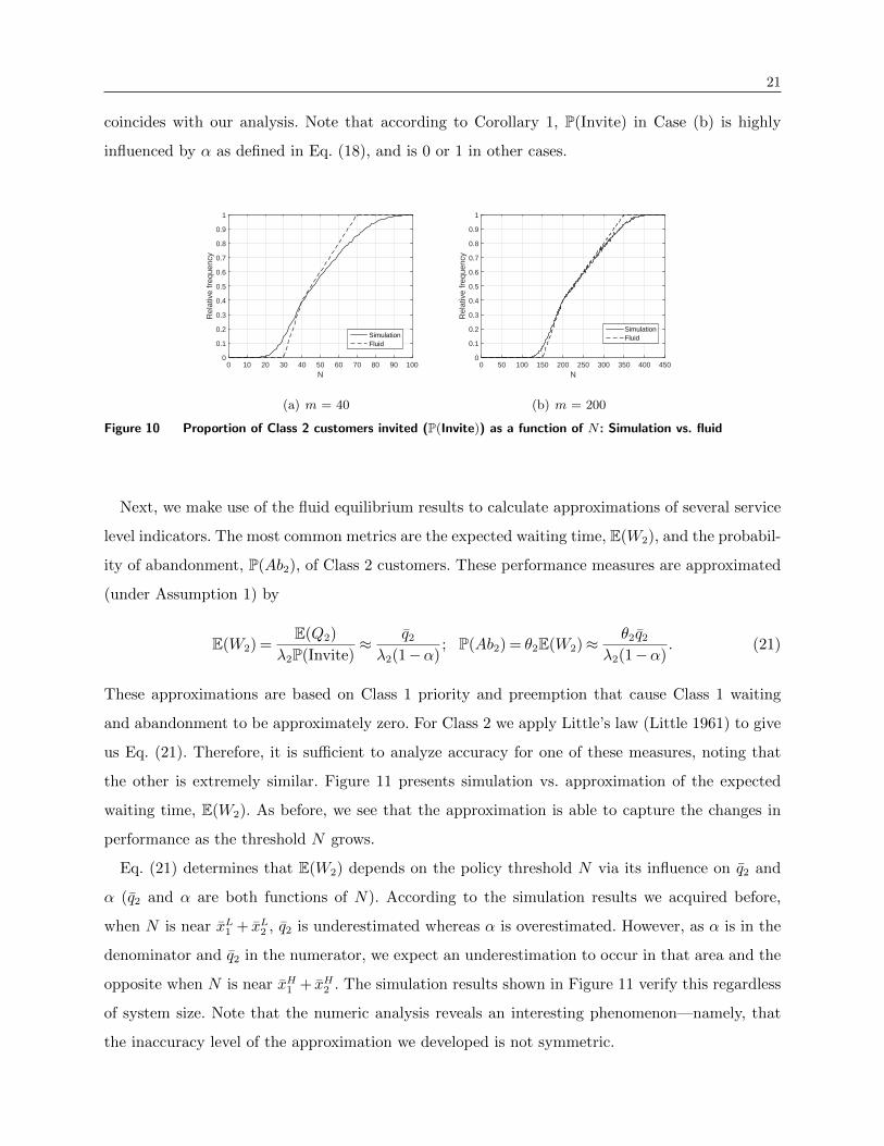
coincides with our analysis. Note that according to Corollary 1, P(Invite) in Case (b) is highly

influenced by α as defined in Eq. (18), and is 0 or 1 in other cases.

N0 10 20 30 40 50 60 70 80 90 100

Rel

ativ

e fr

eque

ncy

0

0.1

0.2

0.3

0.4

0.5

0.6

0.7

0.8

0.9

1

SimulationFluid

(a) m = 40

N0 50 100 150 200 250 300 350 400 450

Rel

ativ

e fr

eque

ncy

0

0.1

0.2

0.3

0.4

0.5

0.6

0.7

0.8

0.9

1

SimulationFluid

(b) m = 200

Figure 10 Proportion of Class 2 customers invited (P(Invite)) as a function of N : Simulation vs. fluid

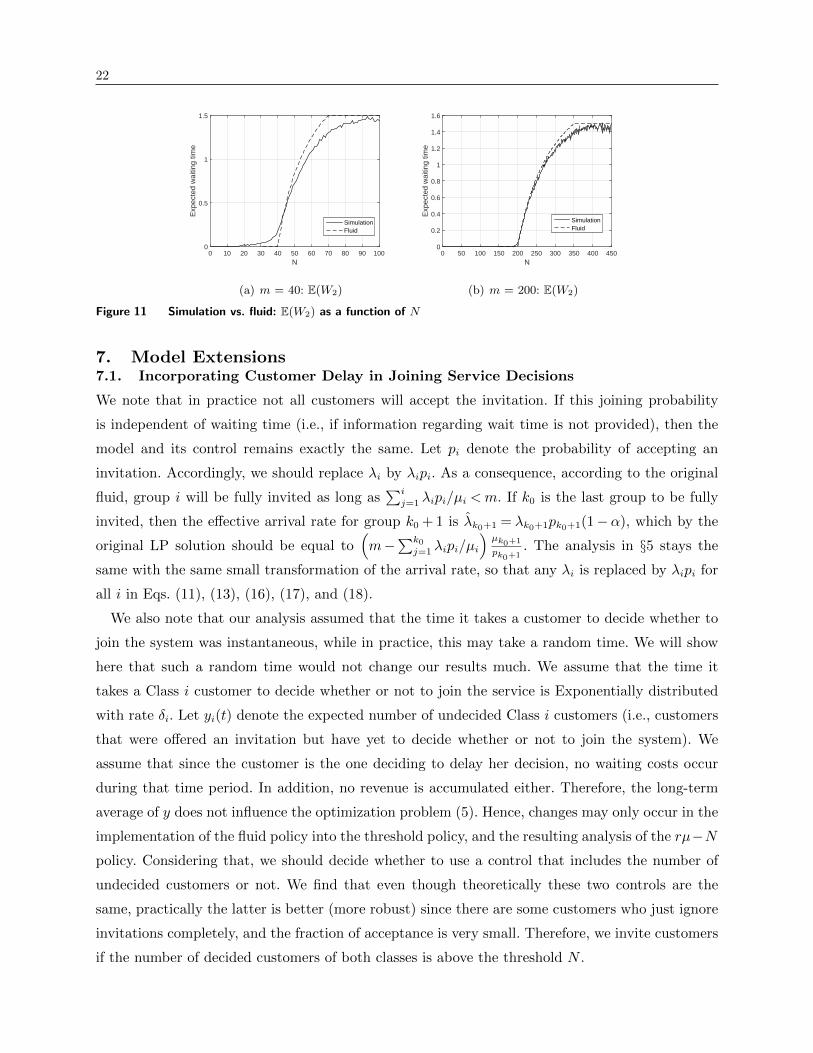
Next, we make use of the fluid equilibrium results to calculate approximations of several service

level indicators. The most common metrics are the expected waiting time, E(W2), and the probabil-

ity of abandonment, P(Ab2), of Class 2 customers. These performance measures are approximated

(under Assumption 1) by

E(W2) =E(Q2)

λ2P(Invite)≈ q2λ2(1−α)

; P(Ab2) = θ2E(W2)≈θ2q2

λ2(1−α). (21)

These approximations are based on Class 1 priority and preemption that cause Class 1 waiting

and abandonment to be approximately zero. For Class 2 we apply Little’s law (Little 1961) to give

us Eq. (21). Therefore, it is sufficient to analyze accuracy for one of these measures, noting that

the other is extremely similar. Figure 11 presents simulation vs. approximation of the expected

waiting time, E(W2). As before, we see that the approximation is able to capture the changes in

performance as the threshold N grows.

Eq. (21) determines that E(W2) depends on the policy threshold N via its influence on q2 and

α (q2 and α are both functions of N). According to the simulation results we acquired before,

when N is near xL1 + xL2 , q2 is underestimated whereas α is overestimated. However, as α is in the

denominator and q2 in the numerator, we expect an underestimation to occur in that area and the

opposite when N is near xH1 + xH2 . The simulation results shown in Figure 11 verify this regardless

of system size. Note that the numeric analysis reveals an interesting phenomenon—namely, that

the inaccuracy level of the approximation we developed is not symmetric.

22

N0 10 20 30 40 50 60 70 80 90 100

Exp

ecte

d w

aitin

g tim

e

0

0.5

1

1.5

SimulationFluid

(a) m = 40: E(W2)

N0 50 100 150 200 250 300 350 400 450

Exp

ecte

d w

aitin

g tim

e

0

0.2

0.4

0.6

0.8

1

1.2

1.4

1.6

SimulationFluid

(b) m = 200: E(W2)

Figure 11 Simulation vs. fluid: E(W2) as a function of N

7. Model Extensions7.1. Incorporating Customer Delay in Joining Service Decisions

We note that in practice not all customers will accept the invitation. If this joining probability

is independent of waiting time (i.e., if information regarding wait time is not provided), then the

model and its control remains exactly the same. Let pi denote the probability of accepting an

invitation. Accordingly, we should replace λi by λipi. As a consequence, according to the original

fluid, group i will be fully invited as long as∑i

j=1 λipi/µi <m. If k0 is the last group to be fully

invited, then the effective arrival rate for group k0 + 1 is λk0+1 = λk0+1pk0+1(1−α), which by the

original LP solution should be equal to(m−

∑k0

j=1 λipi/µi

)µk0+1

pk0+1. The analysis in §5 stays the

same with the same small transformation of the arrival rate, so that any λi is replaced by λipi for

all i in Eqs. (11), (13), (16), (17), and (18).

We also note that our analysis assumed that the time it takes a customer to decide whether to

join the system was instantaneous, while in practice, this may take a random time. We will show

here that such a random time would not change our results much. We assume that the time it

takes a Class i customer to decide whether or not to join the service is Exponentially distributed

with rate δi. Let yi(t) denote the expected number of undecided Class i customers (i.e., customers

that were offered an invitation but have yet to decide whether or not to join the system). We

assume that since the customer is the one deciding to delay her decision, no waiting costs occur

during that time period. In addition, no revenue is accumulated either. Therefore, the long-term

average of y does not influence the optimization problem (5). Hence, changes may only occur in the

implementation of the fluid policy into the threshold policy, and the resulting analysis of the rµ−Npolicy. Considering that, we should decide whether to use a control that includes the number of

undecided customers or not. We find that even though theoretically these two controls are the

same, practically the latter is better (more robust) since there are some customers who just ignore

invitations completely, and the fraction of acceptance is very small. Therefore, we invite customers

if the number of decided customers of both classes is above the threshold N .

23

Therefore, with customer delay and uncertain acceptance of invitation the fluid representation

of our system (9) becomes four-dimensional:

y1(t) = λ1p1− δ1y1(t) (22)

y2(t) = λ2p2Ix1(t)+x2(t)<N− δ2y2(t)

x1(t) = δ1y1(t)−µ1 (x1(t)∧m)− θ1(x1(t)−m)+

x2(t) = δ2y2(t)−µ2

(x2(t)∧ (m−x1(t))

+)− θ2

(x2(t)− (m−x1(t))

+)+

.

It can be easily shown that the steady-state solution to (22) is a vector (y1, y2, x1, x2) where y1 =

λ1p1δ1

, y2 = λ2p2(1−α)δ2

and x1, x2, and α are as stated in Theorem 3 (with any λi multiplied by pi).

Remark 2. A more sophisticated setting is to assume that customer’s decision to join depends

on information provided regarding the expected queue length (or waiting time) as well as the

reward function (see for example Gurvich et al. (2009)). In such a case, the optimization problem

becomes:

max∀zi,qi

∑i∈K

ri(qi)µizi− ciqi (23)

s.t.∑i∈K

zi ≤m

µizi + θiqi ≤ λipi(qi), ∀i∈K

zi, qi ≥ 0, ∀i∈K.

If we assume the following reasonable assumptions: i) the acceptance probability function pi(·) is a

decreasing continuous function of qi that converges to zero as load increases, i.e., limqi→∞ pi(qi) =

0, and we set a basic probability of invitation acceptance pi such that pi := pi(0) ≤ 1; ii) the

reward function ri(·) is also a decreasing function of system load such that ri = limqi↓0 ri(qi) and

limqi→∞ ri(qi) = −∞ (the latter indicates that it is better to not invite than invite and never to

serve), then the solution to (23) model would be the same as when the customer’s choice to join is

independent of the system load.

However, we note that if one implements the LP solution via a threshold policy, the resulted fluid

approximation in this case will become an ODE with state-dependent parameters, whose stationary

solution is harder to compute. It will be a solution to a fixed point equation, such as the one

analyzed in Armony et al. (2009), Gurvich et al. (2009). We leave this to future research.

7.2. Applying Invitation Policy in a Time-Varying Environment

In practice, the arrival rate for each class may change over time as well as staffing. This may result

in a need to change the thresholds over time to accommodate the changing offered-load of each

24

group. We propose to use time discretization approximation, such as the well known Pointwise

Stationary Approximation (PSA) and the Stationary Independent Period-by-Period (SIPP) that

are used for staffing decisions (Green et al. 2007)). Accordingly, the day is divided into relatively

homogeneous time intervals (e.g., an hour) assuming a constant arrival rate within the interval.

Then, for each individual time interval, we identify its associated critical group and set a threshold.

Let τ be the time interval (τ ∈ 1, ..., T). Denote by kτ0 the critical service group for time interval

τ , so that all customer groups 1, ..., k0 are fully invited. Hence,

kτ0 = maxj∈κ

j :mτ ≤

λτjµτj

For example, for the offered load functions presented in Figure 12, kτ0 = 2 for τ ∈ 7, ..,10,16, ..,19

and 1 for all other time intervals. Hence, we may re-calibrate the equivalent 2-class system param-

eters according to Remark 1 for each time interval. This will necessitate some adjustments to

Equations (1), (13), and Theorem 3 that are given explicitly in Appendix D.

The above procedure results in P(Inviteτkτ0+1) = 1−ατ , for j ≤ kτ0 , P(Inviteτj ) = 1 and for j > kτ0 +1,

P(Inviteτkτ0+1) = 0. The performance level for each group will change over time in the following way:

P(Abτj ) = 0 and E(W τj ) = 0 for the all invited groups—j ≤ kτ0—at time interval τ . For group kτ0 + 1

we have

E(W τkτ0+1) =

E(Qkτ0+1)

λkτ0+1P(Inviteτkτ0+1)≈

qkτ0+1

λτkτ0+1(1−ατ );

P(Abτkτ0+1) = θkτ0+1E(W τkτ0+1)≈

θk0+1qk0+1

λτkτ0+1(1−ατ ).

Groups j > kτ0 + 1 are not invited at time interval τ ; therefore, they don’t really have any perfor-

mance measure at that time.

In practice, this procedure will result in a series of threshold N τ = (N τ1 ,N

τ2 , ...N

τk ) that change

over time so that N τj =∞ for j ≤ kτ0 , N τ

j = −1 for j ≥ kτ0 + 1 (any negative threshold value will

result in zero invitations since Q(t)≥ 0), and one finite threshold 0≤N τkτ0+1 <∞ regulating arrival

rate at time interval τ . Determining that threshold value could be done by either a specific class

performance measure or by aggregating performance over all classes. The weighted average service

level across all customers invited at time interval τ is

E(W τ ) =

kτ0+1∑j=1

λτjP(Inviteτj )∑kτ0+1

k=1 λτkP(Inviteτk)E(W τ

j ); P(Abτ ) =

kτ0+1∑j=1

λτjP(Inviteτj )∑kτ0+1

k=1 λτkP(Inviteτk)P(Abτj ).

25

0

20

40

60

80

100

120

0

20

40

60

80

100

120

1 2 3 4 5 6 7 8 9 10 11 12 13 14 15 16 17 18 19 20 21 22 23 24

Num

ber o

f Age

nts

Cum

ulat

ive

Offe

red

Load

Time

R1(t)R2(t)R3(t)m(t)

Figure 12 Example of time-varying offered load and staffing

8. Case Study: Applying Invitation Policy in a Contact Center

In this section, we analyze real data taken from an existing proactive service system in the context

of customer web-services. We aim to compare the effectiveness of our proposed policy as well as

demonstrate the importance of using one. Naturally, this real system is more complex than our

model which gives rise to some challenges in parameter estimation and adjustments that should

be done.

The customer data set comprises more than half a million chats of a transportation company

over one month. This company website provides both service and sale support through its contact

center with 30 service agents (working in shifts, so that there are around 9 active agents each

hour). The system traces online customers and computes a score that indicates the “importance”

of providing help to that customer—that score is based on their browsing behavior. (For example,

a customer that receives errors in the checkout process of a purchase process is a classic high-

score customer.) According to the customer score and chat service capacity, the system may send

invitations to high-score customers. An analysis of the score distribution allows us to cluster the

customers into 5 different classes as shown in Figure 1. The most intriguing class is the class with

score 0. This class includes customers which the system has no information on and consists of a

third of the population.

Upon receiving an invitations for service, the customers decide whether or not to accept it. Once

accepting the invitation, customers start to wait in a queue until the system detects an available

server and assigns this customer to that server. Customers have finite patience; hence, they may

abandon the queue before they are assigned to a server. Before a chat session is over, customers

may purchase commodities from the company, which we will refer to as conversion. In this analysis,

we consider the conversion rate, which is the proportion of customers purchasing commodities, as

the main output of the service. We collected 520,727 chats that were served during January 2016.

Each of them stands for an invited customer on this website. By screening the data, 154 error chats

are excluded because of technical failure; 95.3% of the remaining 520,537 invitations are ignored by

26

the customers. Out of those who accepted an invitation, 17.3% abandon the queue. Finally, there

are only 20,202 customers entering service.

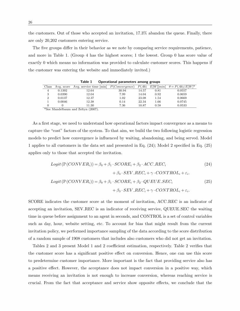
The five groups differ in their behavior as we note by comparing service requirements, patience,

and more in Table 1. (Group 4 has the highest scores; 1 the lowest. Group 0 has score value of

exactly 0 which means no information was provided to calculate customer scores. This happens if

the customer was entering the website and immediately invited.)

Table 1 Operational parameters among groups

Class Avg. score Avg. service time [min] P (Convergence) P (Ab) E[W ][min] θ= P (Ab)/E[W ]*4 0.1392 12.64 30.94 14.57 0.81 0.05573 0.0390 12.04 7.99 14.04 0.92 0.06592 0.0137 12.37 1.02 23.08 1.54 0.06691 0.0046 12.38 0.14 22.34 1.66 0.07450 0 11.30 7.36 10.87 0.58 0.0533

*See Mandelbaum and Zeltyn (2007).

As a first stage, we need to understand how operational factors impact convergence as a means to

capture the “cost” factors of the system. To that aim, we build the two following logistic regression

models to predict how convergence is influenced by waiting, abandoning, and being served. Model

1 applies to all customers in the data set and presented in Eq. (24); Model 2 specified in Eq. (25)

applies only to those that accepted the invitation.

Logit (P (CONV ERi)) = β0 +β1 ·SCOREi +β2 ·ACC RECi (24)

+β3 ·SEV RECi + γ ·CONTROLi + εi.

Logit (P (CONV ERi)) = β0 +β1 ·SCOREi +β2 ·QUEUE SECi (25)

+β3 ·SEV RECi + γ ·CONTROLi + εi.

SCORE indicates the customer score at the moment of invitation, ACC REC is an indicator of

accepting an invitation, SEV REC is an indicator of receiving service, QUEUE SEC the waiting

time in queue before assignment to an agent in seconds, and CONTROL is a set of control variables

such as day, hour, website setting, etc. To account for bias that might result from the current

invitation policy, we performed importance sampling of the data according to the score distribution

of a random sample of 1908 customers that includes also customers who did not get an invitation.

Tables 2 and 3 present Model 1 and 2 coefficient estimation, respectively. Table 2 verifies that

the customer score has a significant positive effect on conversion. Hence, one can use this score

to predetermine customer importance. More important is the fact that providing service also has

a positive effect. However, the acceptance does not impact conversion in a positive way, which

means receiving an invitation is not enough to increase conversion, whereas reaching service is

crucial. From the fact that acceptance and service show opposite effects, we conclude that the

27

abandonments have negative influence on conversion. According to Table 3, the longer a customer

waits in queue, the lesser the chance she will make a purchase during her visit (regardless of whether

she was served or had abandoned). In numbers, waiting 1 more minute (60 seconds) will decrease

the odd ratio of the probability of conversion by 9.15%.

Table 2 Model 1: Including all invited customers

Estimate Std. Error z value Pr(>|z|)SCORE 24.849 0.3115 79.77 <2e-16∗∗∗

ACC REC -0.586 0.1692 -3.46 0.00053∗∗∗

SEV REC 0.446 0.1799 2.48 0.01313∗

CONTROL includedn= 520,573, ∗p<0.1; ∗∗p<0.05; ∗∗∗p<0.01

Table 3 Model 2: Only customers who accept an invitation are included

Estimate Std. Error z value Pr(>|z|)SCORE 22.912 1.0441 21.95 <2e-16∗∗∗

QUEUE SEC -0.0016 0.0006 -2.73 0.0064∗∗∗

SEV REC 0.290 0.1835 1.58 0.1137CONTROL includedn= 24,440, ∗p<0.1; ∗∗p<0.05; ∗∗∗p<0.01

Ideally, we would have ranked the customer classes according to the marginal increase attributed

to the service. However, as we only have data on customers that were invited, we cannot simply use

the conversion rate of non-served customers within this data set to estimate the general conversion

rate of unassisted customers in the entire population. The unserved customers within the dataset

were not served because they declined the invitation (not because they were not offered assistance.)

Accordingly, we used the data as a platform on which to validate our theoretical results, with

the objective of maximizing the conversion rate amongst served customers, i.e., to use the service

capacity we have in the most effective way. We looked at the served customers conversion rate

as the total revenue in our model. We note that with more comprehensive information, one can

easily update r to represent the marginal increase in conversion, which we believe to be a more

appropriate objective.

Using Table 1, we set for each class its relative ranking rµ by considering r as the probability

of conversion (P(CONV ER)) of a single served customer. This results in the following order of

the groups: 4,3,0,2,1. For each possible N (N ∈ 1...20) we calculated the proportion of invited

customers for each class, using the parameter α according to Eq. (18), the number of customers

in the system, x2, using Eq. (17), and the queue length, q2, using Eq. (8). We then estimated the

expected wait and abandonment via Eq. (21). Finally, we evaluated the performance of that policy

by estimating the conversion rate. For that purpose we used Model 2 that captures the combined

effect of a customer being served or abandoned, and waiting on the probability of conversion

28

for each customer class. Multiplying by the effective service rate under this policy one gets the

conversion rate. In a way, this use of the empirical results creates a refined version of our revenue

maximization function presented in (5), in which the elusive waiting cost is evaluated by its impact

on the probability of conversion. In this case study, we found that the threshold N that maximizes

convergence rate was 8.

Table 4 compares the resulting convergence rate (expected number of customers converging

per minute) between our policy, an ‘invite everyone’ policy in which no specific effort is done

to find the most valuable customers or extending an invitation arbitrarily whenever a server is

idle, and the current policy of the organization which ranks customer only according to the score

(i.e., according to the group numbers). We observe that applying a proactive invitation policy can

increase convergence rates dramatically, and doing so in a right way is important. An important

difference between the proactive policy currently applied by the organization and our policy regards

the consideration of Group 0 (no-information) customers. We rank these customers higher than

Groups 1 and 2, i.e., we suggest inviting an unknown customer over a customer of a lower class.

We think that this case study also raises some interesting questions for further extensions of

the model. For example, the data suggest that customer scores in this environment are a dynamic

measure, that may become more accurate as time progresses. Taking into account inaccuracy in

value estimation may prove to be important. In a way, our decision to prioritize the no-information

class (Group 0) over some of the other groups, could be viewed as including score uncertainty in

the expected revenue score, r. This proved to be important.

Table 4 Operational parameters among groups

Class rµ valueConvergence rate

rµ− 8Invite

everyoneCurrentpolicy

4 2.738 2.64 0.40 2.243 0.307 4.66 1.01 1.962 0.073 0 0.28 0.171 0.006 0 0.03 0.020 0.339 0.56 0.86 0.98

Sum 7.85 2.59 5.37

9. Conclusions, Remarks and Limitations

Inspired by the possibility of utilizing customer data to create a proactive service system, we

undertook the challenge of balancing proactiveness in the face of scarce capacity. To do so, we

constructed a multi-class multi-server model with impatient customers that is able to capture

the trade-off between revenue seeking and service level. We first defined an optimal fluid priority

policy—rµ rule—by solving a linear programming problem that determines the optimal arrival

rate to the system. The rµ rule prioritizes invitations according to the product of revenue and

29

service rate. This fluid policy defines a specific (boundary) class of customers; customers with

higher priority will always be invited, and customers with lower priority will never be invited. This

fluid policy is easily applicable through either determining a constant arrival rate for the boundary

class, or by applying a threshold policy to control the flow of that class of customers. We then

extend our fluid model to capture more refined levels of threshold (not just N =m).

We proved that the refined system fluid relaxation has a globally asymptotically stable equilib-

rium. We define that equilibrium, and use it to approximate several performance measures. All

approximations perform well, especially in large systems. Note that we discussed the equilibrium

under a preemptive assumption. Such an assumption is realistic in chat services, as an agent is

serving multiple customers simultaneously, and can put on hold the low-ranking customers. How-

ever, in a system with face-to-face service, preemption is impractical. Nevertheless, in many cases

preemptive and non-preemptive policies converge to the same equilibrium when size goes to infin-

ity (Atar et al. 2010). However, differences appear when the system is critically loaded; such a

situation may not be exceptional. Thus, it is worthy to examine closely the non-preemptive case

in future research. Another assumption we used is a prioritized queue. Again, this is the common

practice in contact centers, but can prove problematic in other environments, such as Healthcare

systems. Thus, it is important to develop policies for FCFS queues as well.

We would like also to refer to our assumption of a defined and discrete set of customer classes,

where, as in reality, customers’ scores may be continuous (see Figure 1). We don’t find this difference

very restrictive for three reasons. 1. Companies use predictive models to evaluate customers’ scores.

To do so, they cluster each customer with other customers that demonstrated similar behavior.

Accordingly, customers are naturally clustered by the scoring evaluation systems anyway. 2. The

ranking itself is evaluated based upon parameters, such as service time and patience. Estimating

parameters correctly for too many score levels, with only a few records per customer group, will

make the ranking imprecise. Therefore, determining a finite number of groups makes practical sense.

3. Our model does not limit the number of classes rendered. Therefore, if technology progresses,

and prediction becomes better, one can create as many finite groups as required.

Finally, we note that an interesting problem would be to prove that indeed the rµ−N policy is

asymptotically optimal. We conjecture that this is indeed the case if the threshold is chosen so that

N is in an order of the square root of total arrival rate of the invited customers (Λ =∑k0+1

i=1 λi). We

leave such proof to future research. The intuition behind that conjecture is that if the threshold is

of that order, then the queue length behaves somewhat like an M/M/m/N+M queue in which the

expected wait is of order 1/√

Λ (Dong et al. 2015). Therefore, queues are very small, as is assumed

by the LP solutions.

30

Acknowledgement

We thank LivePerson Inc. and Michael Natapov for providing data for this research; to Leor Gru-

endlinger and Shlomo Lahav for initiating the collaboration between the Technion and LivePerson;

to Ella Nadjharov, Igor Gavako and late Dr. Valery Trofimov, the dedicated team of the SEELab

at the Technion, for managing the data resources and prepare them for research.

References

Afeche P, Araghi M, Baron O (2017) Customer acquisition, retention, and service access quality: Optimal

advertising, capacity level, and capacity allocation. Manufacturing & Service Operations Management

19(4):674–691.

Armony M, Shimkin N, Whitt W (2009) The impact of delay announcements in many-server queues with

abandonment. Operations Research 57(1):66–81.

Atar R, Giat C, Shimkin N (2010) The cµ/θ rule for many-server queues with abandonment. Operations

Research 58(5):1427–1439.

Atar R, Kaspi H, Shimkin N (2013) Fluid limits for many-server systems with reneging under a priority

policy. Mathematics of Operations Research 39(3):672–696.

Atar R, Mandelbaum A, Reiman MI, et al. (2004) Scheduling a multi class queue with many exponential

servers: Asymptotic optimality in heavy traffic. The Annals of Applied Probability 14(3):1084–1134.

Bassamboo A, Randhawa RS (2016) Scheduling homogeneous impatient customers. Management Science

62(7):2129–2147.

Bernardo M, Budd C, Champneys AR, Kowalczyk P (2008) Piecewise-Smooth Dynamical Systems: Theory

and Applications, volume 163 (Springer Science & Business Media).

Chan CW, Yom-Tov GB, Escobar G (2014) When to use speedup: An examination of service systems with

returns. Operations Research 62(2):462–482.

Cui L, Tezcan T (2016) Approximations for chat service systems using many-server diffusion limits. Mathe-

matics of Operations Research 41(3):775–807.

Dong J, Feldman P, Yom-Tov GB (2015) Service systems with slowdowns: Potential failures and proposed

solutions. Operations Research 63(2):305–324.

Filippov AF (1988) Differential equations with discontinuous righthand sides. Arscott F, ed., Mathematics

and its Applications (Soviet series) (Kluwer Academic Publishers).

Green L, Kolesar P, Whitt W (2007) Coping with time-varying demand when setting staffing requirements

for a service system. Production and Operations Management 16(1):13–39.

Guckenheimer J, Holmes P (2002) Nonlinear Oscillations, Dynamical Systems, and Bifurcations of Vector

Fields (Springer).

31

Gurvich I, Armony M, Maglaras C (2009) Cross-selling in a call center with a heterogeneous customer

population. Operations Research 57(2):299–313.

Jacobson EU, Argon NT, Ziya S (2012) Priority assignment in emergency response. Operations Research

60(4):813–832.

Karush W (1939) Minima of functions of several variables with inequalities as side constraints. Master’s

thesis, Dept. of Mathematics, Univ. of Chicago.

Khalil HK (1996) Nonlinear Systems (Prentice-Hall, New Jersey).

Kocaga YL, Ward AR (2010) Admission control for a multi-server queue with abandonment. Queueing

Systems 65(3):275–323.

Koole G, Pot A (2011) Technical note—a note on profit maximization and monotonicity for inbound call

centers. Operations Research 59(5):1304–1308.

Kuhn HW, Tucker AW (1951) Nonlinear programming. Proceedings of the Second Berkeley Symposium on

Mathematical Statistics and Probability, 481–492 (Berkeley, Calif.: University of California Press).

Kumar S, Randhawa R (2010) Exploiting market size in service systems. Manufacturing & Service Operations

Management 12(3):511–526.

Legros B, Jouini O (2019) On the scheduling of operations in a chat contact center. European Journal of

Operational Research 274(1):303–316.

Little JDC (1961) A proof for the queuing formula: L= λW . Operations Research 9(3):383–387.

Luo J, Zhang J (2013) Staffing and control of instant messaging contact centers. Operations Research

61(2):328–343.

Lyapunov AM (1992) The general problem of the stability of motion. International Journal of Control

55(3):531–534.

Maglaras C, Yao J, Zeevi A (2018) Optimal price and delay differentiation in large-scale queueing systems.

Management Science 64(5):1975–2471.

Mandelbaum A, Zeltyn S (2007) Service engineering in action: The palm/erlang-a queue, with applications

to call centers. Spath D, Fhnrich KP, eds., Advances in Services Innovations, 17–48 (Springer-Verlag.).

Miller BL (1969) A queueing reward system with several customer classes. Management Science 16(3):234–

245.

Munkres JR (1997) Analysis on Manifolds (Westview Press).

Olsen TL, Parker RP (2008) Inventory management under market size dynamics. Management Science

54(10):1805–1821.

Perry O, Whitt W (2011) A fluid approximation for service systems responding to unexpected overloads.

Operations Research 59(5):1159–1170.

32

Rafaeli A, Altman D, Gremler DD, Huang MH, Grewal D, Iyer B, Parasuraman A, de Ruyter K (2017) The

future of frontline research: Invited commentaries. Journal of Service Research 20(1):91–99.

Sanders J, Borst S, Janssen A, van Leeuwaarden J (2017) Optimal admission control for many-server systems

with QED-driven revenues. Stochastic Systems 7(2):315–341.

Sethi S, Zhang Q (1995) Multilevel hierarchical decision making in stochastic marketing-production systems.

SIAM J. Control 33(2):528553.

Shadmi E, Flaks-Manov N, Hoshen M, Goldman O, Bitterman H, Balicer RD (2015) Predicting 30-day

readmissions with preadmission electronic health record data. Medical Care 53(3):283–289.

Shadmi E, Zeltzer D, Flaks-Manov N, Einav L, Balicer R (2017) Reducing readdmision rates: Evidence from

large intervention in Israel. Engelbrecht R, Balicer R, Hercigonja-Szekeres M, eds., The Practice of

Patient Centered Care: Empowering and Engaging Patients in the Digital Era, volume 244, 109–110

(IOS Press).

Tezcan T, Zhang J (2014) Routing and staffing in customer service chat systems with impatient customers.

Operations Research 62(4):943–956.

Ward AR, Kumar S (2008) Asymptotically optimal admission control of a queue with impatient customers.

Mathematics of Operations Research 33(1):167–202.

Weerasinghe A, Mandelbaum A (2013) Abandonment versus blocking in many-server queues: asymptotic

optimality in the QED regime. Queueing Systems 75(2-4):279–337.

Wolff RW (1982) Poisson arrivals see time averages. Operations Research 30(2):223–231.

Yom-Tov GB, Ashtar S, Altman D, Natapov M, Barkay N, Westphal M, Rafaeli A (2018) Customer sentiment

in web-based service interactions: Automated analyses and new insights. WWW 18 Companion: The

2018 Web Conference Companion. April 23–27, 2018, Lyon, France. (ACM, New York, NY, USA).

Yom-Tov GB, Chan CW (2018) Balancing admission control, speedup, and waiting in service systems,

working paper, Technion.

Yoon S, Lewis ME (2004) Optimal pricing and admission control in a queueing system with periodically

varying parameters. Queueing Systems 47(3):177–199.

Zayas-Caban G, Lewis ME (2017) Admission control in a two class loss system with periodically varying

parameters and abandonments, working paper, Cornell.

ec1

Online Appendix: Proofs

Appendix A: Proof of Theorem 1

xL defined by (11) is an equilibrium of system (10) since it’s the only solution to x = 0. In order to show

that it is globally asymptotically stable, we use the following Lyapunov function (Lyapunov 1992): V (x) =

|x1− xL1 |+ |x2− xL2 | . We show that, ∀x 6= xL, V (x) < 0. To do so, we represent xi 6= xLi as xLi + εi where

εi 6= 0. Note that according to Eq. (11), xL2 = 0; thus, ε2 > 0 and |x2− xL2 | = ε2. We also make use of the

following sign indicator to avoid the absolute value of |x1− xL1 |: ζ =

1, ε1 ≥ 0−1, ε1 < 0.

Accordingly, using Eq. (10) with xL2 = 0 and ε2 > 0, we get:

V (x) = ζx1 + x2 = ζ(λ1−µ1

((xL1 + ε1

)∧m

)− θ1

(xL1 + ε1−m

)+)−µ2

(ε2 ∧

(m−

(xL1 + ε1

))+)− θ2

(ε2−

(m−

(xL1 + ε1

))+)+

. (EC.1)

However, the state space R2+ : x1 > 0, x2 > 0 can be divided into two domains according to the value of

m, and to further domains as a function of the potential volume of Class 1 (λ1/µ1).

Domain A: m< (xL1 + ε1) — In this domain, Eq. (EC.1) becomes:

V (x) = ζ(λ1−µ1m− θ1

(xL1 + ε1−m

))− θ2ε2. (EC.2)

Substituting for xL1 using Eq. (11) we have λ1/µ1 ≤ m < (xL1 + ε1) = λ1/µ1 + ε1, which means that

ε1 > 0 and thus, ζ1 = 1. Since λ1 ≤ µ1m, θ1 > 0 by definition, and (xL1 + ε1−m) > 0 by Domain A,

ζ1 (λ1−µ1m− θ1 (xL1 + ε1−m))< 0. Since θ2 is positive by definition, V (x) in Eq. (EC.2) becomes a sum-

mation of two non-positive elements, (λ1−µ1m− θ1 (xL1 + ε1−m)) and −θ2ε2. Thus, V (x)< 0 for x 6= xL.

Domain B: m ≥ (xL1 + ε1) — In this domain, Eq. (EC.1) becomes: V (x) = ζ (λ1−µ1 (xL1 + ε1)) −

µ2

(ε2 ∧ (m− (xL1 + ε1))

+)− θ2

(ε2− (m− (xL1 + ε1))

+)+

. Since µ2, θ2, ε2, and (m− (xL1 + ε1)) are all pos-

itive and(ε2− (m− (xL1 + ε1))

+)+

is non-negative, we get:

V (x)< ζ (λ1−µ1 (xL1 + ε1)) , for x2 6= xL2V (x) = ζ (λ1−µ1 (xL1 + ε1)) , for x2 = xL2 .

(EC.3)

Substituting for xL1 using Eq. (11), Eq. (EC.3) becomes V (x)≤−ζµ1ε1. Since ζ and ε1 have the same sign

by the definition of ζ and since µ1 is positive by definition, V (x)< 0 for x 6= xL.

Appendix B: Proof of Theorem 2

The dynamics f2(x) (given in (14)) can have three possible forms in different regions of the state space (see

Figure EC.1):

Region A, ΩA := (x1, x2) |x1 ≥m

fA2 (x(t)) := x(t) =

λ1−µ1m− θ1 (x1(t)−m)λ2− θ2x2(t).

(EC.4)

Region B, ΩB := (x1, x2) |x1 <m<x1 +x2

fB2 (x(t)) = x(t)=

λ1−µ1x1(t)λ2−µ2 (m−x1(t))− θ2 (x1(t) +x2(t)−m).

(EC.5)

ec2

Figure EC.1 Regions of system state

Region C, ΩC := (x1, x2) |x1 +x2 ≤m

fC2 (x(t)) = x(t) =

λ1−µ1x1(t)λ2−µ2x2(t).

(EC.6)

Solving f i2(x) = 0 yields that xA =

(λ1+m(θ1−µ1)

θ1λ2

θ2

)is an equilibrium point for fA2 (x), xB =(

λ1

µ1λ2−(µ2−θ2)(m−λ1/µ1)

θ2

)is an equilibrium point for fB2 (x), and xC =

( λ1

µ1λ2

µ2

)is an equilibrium point for fC2 (x).

Since all of the dynamics (EC.4, EC.5, EC.6) are linear and all their eigenvalues are negative, according to

Lyapunov’s stability theorem, these equilibria are all asymptotically stable for each of the dynamics (Khalil

1996); therefore, they are all locally stable for f2(x). We are left to show that for λ1/µ1 ≤m≤ λ1/µ1 +λ2/µ2,

there may be only one admissible equilibrium, and that the flow converges to this domain, regardless of the

starting point.

Definition EC.1. We say that a point x= x is an admissible equilibrium of f2(x) if, for one i∈A,B,C,

x = f i2(x) and x∈Ωi.

By Definition EC.1, an equilibrium x is not admissible if that equilibrium is out of the region of definition.

Clearly, xA and xC are inadmissible under λ1/µ1 <m<λ1/µ1 +λ2/µ2.

xB is admissible under λ1/µ1 < m < λ1/µ1 + λ2/µ2, because then, xB1 = λ1

µ1< m, xB2 =

λ2−(µ2−θ2)(m−λ1/µ1)

θ2= λ2−µ2(m−λ1/µ1)

θ2+m−λ1/µ1 >

λ2−µ2(λ1/µ1+λ2/µ2−λ1/µ1)

θ2+m−λ1/µ1 =m−λ1/µ1.

Accordingly, there is one, and only one, admissible equilibrium; all the other equilibria are non-admissible.

Note also that the equilibrium (13) is asymptotically stable if there are no restrictions on the defining region,

i.e., the dynamics are valid in the entire space. In other words, the trajectory starting inside each region

leaves after a finite time if the equilibrium doesn’t reside there, and flows towards the region in which the

non-admissible equilibrium does reside.

Any flow starting at x∈ΩC will cross to ΩB after a finite time and then converge to xB; any flow starting

at x∈ΩA will cross to ΩB ∪ΩC and then again will converge to xB. Therefore, a flow starting at any point

will enter the domain with the admissible point after a finite time, and once there will converge to that

admissible point which is a locally stable equilibrium, which makes that equilibrium globally stable.

ec3

Appendix C: Proof of Theorem 3

First we need to establish that xL and xH are locally stable equilibria also in (15).

Lemma EC.1. If xL ∈ R1, then xL is a locally stable equilibrium in the original discontinuous ODE

defined in (15).

Proof: This is typical for piecewise-smooth ODEs and follows from Guckenheimer and Holmes (2002). Intu-

itively, in the continuous ODE defined by f1, there exists a small ball around xL such that trajectories that

start within the ball will converge to xL and stay there. If xL is in R1, then one can also select a small ball

around xL such that (1) trajectories that start within the ball will converge to xL and (2) the ball is entirely

contained in R1. Then, starting a trajectory in this small ball, but letting the system dynamics be defined

according to our original, discontinuous ODE in (15), the trajectory will stay in the ball, which means they

will stay in R1 and follow the same dynamics as the continuous ODE f1, since it won’t hit the switching

boundary, Σ, or enter the other region, R2. Thus, xL is locally stable.

Similarly, we claim:

Lemma EC.2. If xH ∈ R2, then xH is a locally stable equilibrium in the original discontinuous ODE

defined in (15).

Next, we analyze the dynamics of the system on the switching boundary, Σ. Denote δN (x)≡ xT∇Σ as the

projection of vector field x on the gradient of Σ. δN (x) indicates whether the flow moves toward or away

from Σ when approached from R1,Σ or R2. More specifically, we look at the forces on either side of the

switching boundary, i.e., the component of fi normal to Σ, which we denote by δi. These measures are often

referred to as the Lie derivatives.

δ1(x1)≡∇ΣT f1 (x1,N −x1)

δ2(x1)≡∇ΣT f2 (x1,N −x1) .

We have the following three cases to consider:

I. δ1(x)< 0 and δ2(x)< 0: a flow that hits Σ will transition from R2 to R1. A flow that starts at R1 will

remain there;

II. δ1(x)δ2(x)< 0: a flow that hits Σ will stay on Σ—potentially forever. The flow is said to be in a sliding

mode, in which x1 +x2 is constant and equal to N ;

III. δ1(x)> 0 and δ2(x)> 0: a flow that hits Σ will transition from R1 to R2. A flow that starts at R2

will remain there.

The importance of Case II is in recognizing the sliding mode that may converge to an additional equilibrium

inside the sliding set. This point is typically not a fixed point in the standard sense since the ODE is nonzero

at that point. However, it is still an equilibrium by Definition 1 because if a flow starts at that point, it

stays there. In some cases, this special equilibrium is unique and stable. We call this type of equilibrium a

pseudo-equilibrium, as in Bernardo et al. (2008).

Definition EC.2 (Pseudo-Equilibrium). We call a point x a pseudo-equilibrium if it is an equilibrium

of the sliding flow, i.e., for some scalar 0<ϕ< 1, f s =ϕf1(x) + (1−ϕ)f2(x) = 0, x∈Σ.

ec4

Note the similarities to the Filippov ODE (15). When the convex combination is active in (15), i.e.,

ϕ∈ [0,1], there exists an equilibrium on the switching boundary Σ.

Lemma EC.3. The point (x1,ϕxL2 + (1− ϕ)xH2 ) is a pseudo-equilibrium when xL1 + xL2 < N < xH1 + xH2 ,

where ϕ= α is given by Eq. (18)

In order to prove EC.3, we need to find the conditions in which a pseudo-equilibrium exists, i.e., Case II

above. Note that xL1 = xH1 under all conditions, and therefore we only need to consider the convex combination

with respect to x2, denoted by f s2 and defined below. (This is the result of the Independence of x1 in x2.)

We distinguish between two ranges of m with respect to N : m≤N and m>N

f s2(ϕ) (0<ϕ< 1) is given by

f s2(ϕ) = λ1−µ1x1 + (1−ϕ)λ2−µ2

((N − x1)

+ ∧ (m− x1))− θ2

((N − x1)

+− (m− x1))+

= (1−ϕ)λ2−µ2

((N − x1)

+ ∧ (m− x1))− θ2

((N − x1)

+− (m− x1))+

. (EC.7)

The last transition is due to x1 being an equilibrium.

We next analyze the value of f s2(ϕ) for four different ranges of N .

• N ≤ x1 =⇒ f s2(ϕ) = (1−ϕ)λ2 > 0.

• x1 < N ≤m =⇒ f s2(ϕ) = (1−ϕ)λ2 − µ2 (N − x1) and 0 < µ2 (N − x1)/λ2 < 1. Therefore, when ϕ =

1−µ2 (N − x1)/λ2, f s2(ϕ) = 0 and ϕ∈ (0,1).

• m < N ≤ (λ2−µ2 (m− x1))/θ2 + m =⇒ f s2(ϕ) = (1−ϕ)λ2 − µ2 (m− x1) − θ2 (N −m) and 0 ≤

(µ2 (m− x1) + θ2 (N −m))/λ2 < 1. Therefore, when ϕ = 1− (µ2 (m− x1) + θ2 (N −m))/λ2, f s2(ϕ) = 0 and

ϕ∈ (0,1).

• N > (λ2−µ2 (m− x1))/θ2 +m =⇒ f s2(ϕ)< 0 for any ϕ∈ (0,1).

Hence, f s2(ϕ) = 0 only if x1 <N ≤ (λ2−µ2 (m− x1))/θ2 +m, in which case ϕ follows Eq. (18).

This finalizes the proof of Lemma EC.3.

We now aim to show that all the equilibria defined are globally asymptotically stable. To do so, we will

analyze the flow. First we claim in the following lemma that under all conditions, regardless of the starting

point, the flow will converge to a strip around x1.

Lemma EC.4. In the system defined by Eq. (9), ∀ε > 0, ∃T > 0, such that x (t > T ) ∈ Rε =

(x1, x2) |x1 ∈ (x1− ε, x1 + ε) , ε > 0 .

To prove this lemma, we use the Lyaponov functions. As x1 dynamics are independent in x2, we analyze a

system with only x1(t). This system is identical to the system in (10) with µ2 = θ2 = 0. Therefore, using the

proof of Theorem 1 in Appendix A, with µ2 = θ2 = 0 proves the global stability of a system that consists of

only Class 1 customers (we omit a comprehensive proof due to redundancy). As seen in Eqs. (13) and (11),

x1 has an equilibrium that depends on the level of load of Class 1 customers only.

x1 = λ1/µ1

Hence, regardless of the starting point, after a finite time the process will converge to a small strip around

x1 as shown in Figure EC.2. We next analyze the behavior of the system within that strip.

ec5

x2

x1 𝒙𝟏

𝑵 − 𝒙𝟏

𝒙𝟏 − 𝜺 𝒙𝟏 + 𝜺

B1

B2

Figure EC.2 Regions of system state when sliding region exists

Let δ(x1,ϕ) be the convex combination of δ1(x1) and δ2(x1), δ(x1,ϕ)≡ϕδ1(x1)+(1−ϕ) δ2(x1), ϕ∈ [0,1] .

Note that δ(x1,0) = δ2(x1), δ(x1,1) = δ1(x1). We evaluate the value of δ(x1,ϕ) at a specific point on Σ,

namely, x1 = x1.

δ(x1,ϕ) = λ1−µ1x1 + (1−ϕ)λ2−µ2

((N − x1)

+ ∧ (m− x1))− θ2

((N − x1)

+− (m− x1))+

= (1−ϕ)λ2−µ2

((N − x1)

+ ∧ (m− x1))− θ2

((N − x1)

+− (m− x1))+

.

The last transition is due to x1 being a stable equilibrium.

We next analyze the value of δ(x1,ϕ) . We distinguish between three different ranges of N . The analysis

is similar to the analysis made for f s, and its results are summarized in Table EC.1.

Table EC.1 Delta function value by range of N

N range δ polarityλ2−µ2(m−λ1/µ1)

θ2+m≤N Case I

λ1µ1<N < λ2−µ2(m−λ1/µ1)

θ2+m Case II

λ1µ1≥N Case III

Note that δ (x1,ϕ) = 0 in Cases I and III only if ϕ= 1 or 0, respectively. Hence, system dynamics on the

border Σ equals f1(x) or f2(x), respectively. Also Σ can be considered to belong to R1 or R2, respectively.

Accordingly, the flow at the breakpoint follows either Case I or Case III.

We use the phase portrait (Figure EC.3) to sketch the system flow. The boundary Σ is plotted by a red

line. The equilibrium is marked by a dot. The arrows represent the derivatives of the system states.

The following Lemma determines that the value of δ is consistent throughout the range of the strip;

therefore, for each condition-case combination the behavior of the flow on the switching boundary will be

the same regardless of the exact point of hitting that plane.

Lemma EC.5. In system (9), if ∀ϕ ∈ [0,1], δ (x1,ϕ) > 0 (or < 0), then ∃ε > 0, such that ∀x1 ∈

(x1− ε, x1 + ε), δ(x1,ϕ)> 0 (or δ(x1,ϕ)< 0) holds for ∀ϕ∈ [0,1].

Proof: We prove the case δ(x1,ϕ) > 0. According to the definition, δ(x1,ϕ) = ϕδ1(x1) + (1−ϕ) δ2(x1).

Since ∀ϕ ∈ [0,1]: δ (x1,ϕ) > 0, δ1(x1) > 0 and δ2(x1) > 0. By continuity, there always exists εH > 0 and

ec6

0 10 20 30 40 50x

1

0

10

20

30

40

50x 2

(a) Case MV(a)

0 10 20 30 40 50 60x

1

0

10

20

30

40

50

60

x 2

(b) Case MV(b)

0 20 40 60 80x

1

0

20

40

60

80

x 2

(c) Case MV(c)

Figure EC.3 Phase portraits of MV condition

εL > 0, such that δ1(x1) > 0 for x1 ∈ (x1− εH , x1 + εH), and δ2(x1) > 0 for x1 ∈ (x1− εL, x1 + εL). Taking

ε= min(εL, εH), one has δ1(x1)> 0 and δ2(x1)> 0 for x1 ∈ (x1− ε, x1 + ε) . Furthermore, δ(x1,ϕ)> 0 since

it is a convex combination of δ1(x1) and δ2(x1).

Lemmas EC.4 and EC.5 imply that under Cases I and III conditions, there always exists a small neighbor-

hood of (x1,N − x1)T , where the system trajectory can only cross Σ in one determined direction. However,

in Case II, Σ becomes uncrossable. In that range, we identified a pseudo-equilibrium for which the following

also holds and defines a sliding region.

Lemma EC.6. In system (9), if ∃ϕ0 ∈ (0,1) such that δ (x1,ϕ0) = 0, then ∃ε > 0 such that for all

x1 ∈ (x1− ε, x1 + ε), δ (x1,ϕ) = 0 has a solution with ϕ∈ (0,1).

Proof: From system dynamics (9), one has∂δ (x1,ϕ)

∂ϕ=−λ2 6= 0. Then, the existence of ϕ as an explicit

function of x1 is guaranteed by the implicit function theorem (Munkres 1997), i.e., there exists ε > 0 for

x1 ∈ (x1− ε, x1 + ε) such that ϕ (x1) satisfies δ (x,ϕ (x1)) = 0. Also, note that ϕ (x1) = ϕ0 and ϕ (x) is

continuous at x1; thus, ϕ (x1)∈ (0,1) for all x1 in a sufficiently small neighborhood of x1.

Next, we show that if the system has a sliding region around x1, the system flow converges to this region

in finite time.

Lemma EC.7. In system (9), if a sliding region exists, then ∃ε > 0, such that ∀x∈B1 (see Figure EC.2),

δN(x)< 0 where

B1 =(x1, x2) |x1 ∈ (x1− ε, x1 + ε)∩R1,

and ∀x∈B2, δN(x)> 0, where

B2 =(x1, x2) |x1 ∈ (x1− ε, x1 + ε)∩R2.

Proof: According to Lemma EC.6, a sliding region exists in Case II. One can easily evaluate that

δ2(x1,N − x1) = γ2 < 0,

δ1(x1,N − x1) = γ1 > 0.

Here γ1 and γ2 are functions of parameters, where

γ1 =−µ2((N ∧m)− x1)+− θ2(N −m)

+

γ2 = λ2−µ2((N ∧m)− x1)+− θ2(N −m)

+

ec7

Hence, any x∈B1 can be written as:

x=

(x1 + ∆xL1N − x1 + ∆xL2

),

and |∆xL1 |< ε and ∆xL2 >−∆xL1 . Similarly, ∀x∈B2 can be written as

x=

(x1 + ∆xH1N − x1 + ∆xH2

),

where |∆xH1 |< ε and ∆xH2 <−∆xH1 . Note also that δN(x) is a linear function of x1 and x2 of the form

δN(x) =

aLx1 + bLx2 + cL , δLN(x), x∈B1

aHx1 + bHx2 + cH , δHN (x), x∈B2,

where aL, aH , bL, bH , cL, and cH represent constants and bL, bH < 0. Thus, ∀x∈B1,

δLN(x) = aLx1 + bLx2 + cL = aL∆xL1 + bL∆xL2 + γL <(∣∣aL∣∣+ ∣∣bL∣∣)ε+ γL,

and ∀x∈B2,

δHN (x) = aHx1 + bHx2 + c= aH∆xH1 + bH∆xH2 + γH >−(∣∣aH∣∣+ ∣∣bH∣∣)ε+ γH .

Thus, one can choose

ε= min

(−γL

2 (|aL|+ |bL|),

γH

2 (|aH |+ |bH |)

),

such that

δN(x) = δLN(x)<γL

2< 0, if x∈B2

δN(x) = δHN (x)>γH

2> 0, if x∈B1.

.

Lemma EC.7 shows that, in all Case II, there exists an ε > 0, such that ∀x∈ (x1, x2) |x1 ∈ (x1− ε, x1 + ε),the system state converges to Σ in finite time.

Now we finalize the proof of Theorem 3:

Proof: The system can be categorized into two types: there exists /does not exist a sliding region on Σ

which contains (x1,N − x1).

A. The sliding region does not exist

From Lemma EC.5, we know that there exists εNSR > 0; all the trajectories inside the region BNSR =

(x1, x2) |x1 ∈ (x1− εNSR, x1 + εNSR), can only pass through Σ in one direction. According to Lemma EC.4,

any trajectory arrives to BNSR in finite time. Similarly to the proof of Theorems 1 and 2, all the trajectories

inside BNSR converge to xL (xH). Therefore, in Case (a), xL is a globally asymptotically stable equilibrium,

and in Case (c), xL is a globally asymptotically stable equilibrium.

B. The sliding region exists

From Lemma EC.6, we know that there exists εSR > 0, such that BSR ∩ S is a sliding region, where

BSR = (x1, x2) |x1 ∈ (x1− εSR1, x1 + εSR1). Meanwhile, from Lemma EC.4, we know that all the trajectories

reach BSR in finite time. Lemma EC.7 maintains that all the trajectories inside BSR reach Σ in finite time. In

addition, on the sliding region, evolution of the system state is always along Σ, namely, x1 +x2 =N always

holds. Since x1 converges to x1, all the trajectories will converge to (x1,N − x1).The value of α in Eq. (18)

was calculated to satisfy xG = (x1,N − x1)T , where xG is given in Eq. (17). Therefore, in Case (b), xG is the

globally asymptotically stable equilibrium.

ec8

Appendix D: Equilibrium of time varying system

Let Γτ =∑kτ0

j=1

λτj

µτj

be the total offered load of the fully invited service groups.

Theorem EC.1. At time interval τ the system fluid converges to:

xτ =

xL, if N τ

kτ0 +1 ≤∑

jxLj ;

xG, if∑

jxLj ≤N τ

kτ0 +1 ≤∑

jxHj ;

xH , if∑

jxHj ≤N τ

kτ0 +1,

where

xL =

(λτ1µτ1, ...

λτkτ0µτkτ0

,0, ...,0

),

xG =

(λτ1µτ1, ...,

λτkτ0µτkτ0

,λkτ0 +1(1−ατ )−

(µkτ0 +1− θkτ0 +1

)(mτ −Γτ )

θkτ0 +1

,0, ...,0

),

xH =

(λτ1µτ1, ...,

λτkτ0µτkτ0

,λkτ0 +1−

(µkτ0 +1− θkτ0 +1

)(mτ −Γτ )

θkτ0 +1

,0, ...,0

)and

1−ατ =

µkτ0+1(mτ−Γτ )+θkτ0+1(Nτ−mτ )

λkτ0+1, if mτ <N τ ;

µkτ0+1(Nτ−Γτ )

λkτ0+1, if N τ ≤mτ .