AN INVESTIGATION OF THE EFFECT OF MOBILE NUMBER PORTABILITY ON MARKET COMPETITION

by

Yuriy Podvysotskiy

A thesis submitted in partial fulfillment of the requirements for the degree of

Master of Arts in Economics

EERC MA Program in Economics

National University Kyiv-Mohyla Academy

2006

Approved by ___________________________________________________ Chairperson of Supervisory Committee

__________________________________________________

__________________________________________________

__________________________________________________

Program Authorized to Offer Degree _________________________________________________

Date __________________________________________________________

National University of “Kyiv-Mohyla Academy”

Economics Education and Research Consortium

Abstract

AN INVESTIGATION OF THE EFFECT OF MOBILE NUMBER PORTABILITY ON MARKET COMPETITION

by Yuriy Podvysotskiy

Chairperson of the Supervisory Committee: Professor Roy Gardner Department of Science

This thesis examines possible affects of implementation of technology known as

mobile number portability (MNP) on market competition. Previously it was

strongly believed that MNP leads to improvement of market competition, but

recently several papers argued that.

This work developed theoretical model aplicable for investigation of the effect of

MNP under different market parameters such as growth rate and interconnection

costs.

Arellano-Bond GMM model was used to estimate empirically the effects

described in theoreical literature on switching costs and also the ways that MNP

changes these effects. Original cross-country firm-level panel data was used for

the estimation. Empirical results provide theoretical evidence, besides, estimated

model is transformed into a rule that could be applied for testing possible effect

of MNP on market competition.

ii

TABLE OF CONTENTS

List of Figures and Tables………………………………………………………i

Acknowledgements ……………………………………………………………ii

Glossary …………………………………………………… ……………….iii

Chapter I: Introduction ………………………………………………………..1 Chapter II: Literature Review ………………………………………………….4 Chapter III: Methodology ……………………………………………………13 Chapter IV: Data Description …………………………………………… …21 Chapter V: Estimation Results ………………………………………………..27 Chapter VI: Conclusions ……………………………………………………..42 List of References ……………………………………………………………43 ANNEXES …………………………………………………………………46

iii

LIST OF TABLES

Number Page

1. Geography of the data in the sample……………………………..23

2. Primary Data Description………………………………………..23

3. Summary Statistics of Secondary Variables……………….…..…..24

4. Summary Statistics of Differences of Prices and Market Shares…..25

5. Summary Statistics of Joint Shares of not Included Small Players....26

6. Expectations of Signs of Explanatory Variables …………………35

7. Estimation Results for Main Specifications of the Model…………35

LIST OF FIGURES

Number Page

1. Evolution of Market Share Spreads …..………………………….....2

2. Dependence of required Difference of Market Shares on Market

Parameters (market penetration 60%)..……………………………..40

3. Dependence of required Difference of Market Shares on Market

Parameters (market penetration 80%)………………………………41

4. Evolution of Market Shares under MNP……………………………46

5. Evolution of Per-Minute Prices under MNP…………………..48

iv

ACKNOWLEDGMENTS

I wish to express my dearest gratitude to my supervisor Dr. Roy Gardner for his

inspiration, insightful advice and responsiveness. I am also very thankful to Dr.

Tom Coupe for his valuable comments, criticism and recommendations.

I would like to thank my dear friend and colleague Tamara Konoreva for her

patient listening to my ideas and helpful recommendations.

Also, I would like to express gratitude and respect to my colleagues Olexandr

Lytvyn and Sofia Husenko for providing the excellent competitive environment,

without which this thesis would be impossible.

v

GLOSSARY

Balanced calling pattern - the percentage of calls originating on a network and completed on the same network equals to the percentage of consumers subscribed to this network.

Interconnection costs – arise when mobile carriers charge lower usage fees for calls within the same networks than or calls between the networks.

Key Performance Indicators (KPI) – indicators of operational performance of a mobile carrier, disclosed on regularly (quarterly, semiannually, or annually). Among them usually are ARPU (average revenue per user), MOU (minutes of usage per user), Churn (percentage of customers that switched), Number of subscribers.

Mobile Number Portability (MNP) – regulatory policy that allows consumers to retain the same phone numbers when they switch service providers.

One-way access – refers to a setting with one firm monopolizing input(s) needed by all firms in more competitive sector (e.g. gas and electricity supply).

Two-way access – denotes competing networks, each with its own subscribers, and firms need to purchase vital inputs (services) from each other.

National regulatory authority (NRA) – used as general term denoting a governmental structure responsible for regulation of telecommunications industry in a country.

Number prefix – the first three digits of a mobile number. In absence of MNP number prefix indicates the network of the person being called. Under MNP number prefix has no indicative meaning.

On-network – an adjective denoting calls made by a customer of some network to a customers belonging to the same network.

Off-network – an adjective denoting calls made by a customer of some network to customers belonging to another (competing) network.

Reciprocal access pricing – a network pays as much for termination of a call on the rival network as it receives for completing a call originated on the rival network.

Switching costs – costs that consumers have to bear when they switch from one provider (or product/service) to an alternative.

1

C h a p t e r 1

INTRODUCTION

After switching costs were discovered and described in academic literature

regulators in many industries became preoccupied with finding the ways to either

decrease or eliminate switching costs that was considered a great impediment to

competition.

In particular, national regulatory authorities (NRAs) in telecommunications

industry began to actively discuss and even implement the regulation known as

mobile number portability (MNP). The goal of MNP implementation is decrease

in the consumer switching costs. In this way, it is believed, that after reduction in

switching costs, competition among the mobile carriers would increase.

Concern about impact of MNP on evolution of market shares of competing

mobile carriers was firstly expressed by Shi, 2002. He noticed that after MNP

implementation in Hong-Kong market shares of the competing firms did not

converge, but even started to diverge. Mergers and takeovers became more likely

among mobile operators and competition is more likely to deteriorate.

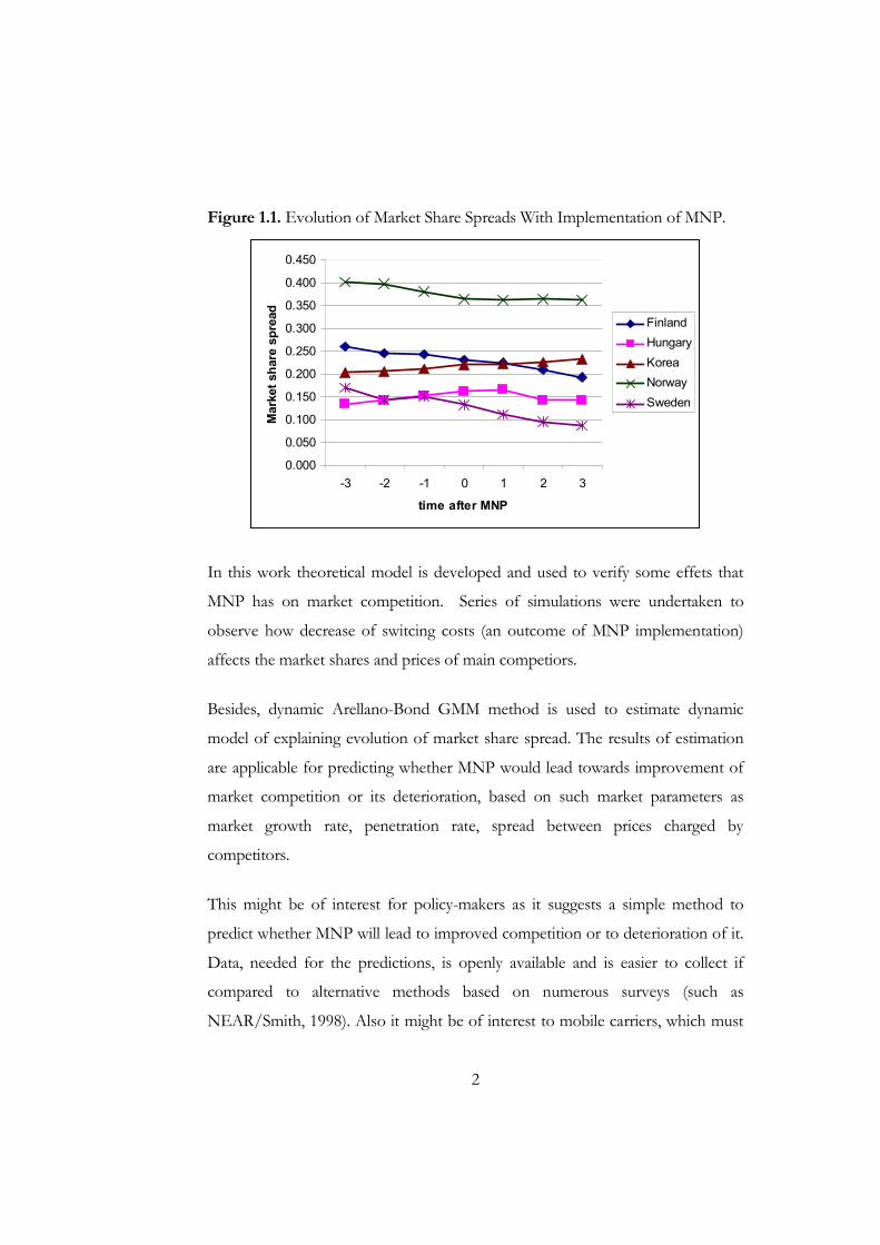
Figure 1.1. below shows the evolution of differences between market shares of

the largest firm and its closest competitors during 3 quarters before and 3

quarters after MNP implementation. Hardly is there any evidence that MNP leads

to improved competition – in Sweden and Finland difference between market

shares of the two largest competitors indeed started to decrease, but in Korea it

started to increase, whereas in Norway and Hungary the behavior is unclear.

2

Figure 1.1. Evolution of Market Share Spreads With Implementation of MNP.

0.000

0.050

0.100

0.150

0.200

0.250

0.300

0.350

0.400

0.450

-3 -2 -1 0 1 2 3

time after MNP

Market share spread

Finland

Hungary

Korea

Norway

Sweden

In this work theoretical model is developed and used to verify some effets that

MNP has on market competition. Series of simulations were undertaken to

observe how decrease of switcing costs (an outcome of MNP implementation)

affects the market shares and prices of main competiors.

Besides, dynamic Arellano-Bond GMM method is used to estimate dynamic

model of explaining evolution of market share spread. The results of estimation

are applicable for predicting whether MNP would lead towards improvement of

market competition or its deterioration, based on such market parameters as

market growth rate, penetration rate, spread between prices charged by

competitors.

This might be of interest for policy-makers as it suggests a simple method to

predict whether MNP will lead to improved competition or to deterioration of it.

Data, needed for the predictions, is openly available and is easier to collect if

compared to alternative methods based on numerous surveys (such as

NEAR/Smith, 1998). Also it might be of interest to mobile carriers, which must

3

be also very interested in the question how market competition is affected by

MNP.

The empirical investigation conducted in this paper supports theoretical

predictions of previous studies. Namely, such theoretical suggestions were

empirically supported as, first, that firms with initially larger market shares have

advantage in maintaining larger size of their network in the future, second, that

larger price differences between larger and smaller competitors leads towards

faster convergence of market shares, third, that higher market growth rates and

low penetration rates characterizing the market lead towards slower convergence,

and even divergence of the market shares is possible.

I found out that MNP is more likely to lead towards improvement of

competition when market is saturated, growing slowly, or when smaller

competitor sells at large discount as compared to the large one. And on quickly

growing markets with low penetration rates MNP may lead to adverse effect on

competition.

The reminder of the paper is organized in the following way. Chapter 2

introduces to empirical and theoretical studies considering MNP and such related

issues as competition in network industries and competition on markets with

switching costs. In Chapter 3 theoretical model setup is provided. Chapter 4

provides data description. Chapter 5 describes the empirical investigation

conducted with the main goal of developing a method to predict whether MNP

will have positive or negative effect on market competition. Chapter 6 concludes.

4

C h a p t e r 2

LITERATURE REVIEW

So far no single theory emerged to explain competition in mobile

telecommunications and to analyze possible outcomes of implementation of

Mobile Number Portability. But there are advances of theory in some tightly

related areas which provide the necessary framework to analyze the problem

through.

The structure of this review is as follows. Recent papers that investigate the

issue of MNP directly are reviewed first. Then the research that created

foundation for the analysis of MNP and telecommunication is described. Also,

relevant empirical methodology and interesting findings of empirical

investigations are discussed.

2.1. Theoretical Developments

So far only few theoretical papers concerned the problem of MNP

implementation directly. All these papers develop from the framework of

network competition, as provided by Armstrong, 1998, and Laffont et al., 1998,

which are describe below, mostly by adding switching costs to the model.

Aoki and Small (2005) is the most frequently cited paper that directly

investigates the effect of MNP implementation. This work gave the interpretation

to MNP as a reduction in switching costs accompanied by increase in fixed and

marginal costs of the firms. Their analytical investigation is focused on the MNP-

caused welfare change of consumers and producers. The model is not

convenient for analysis of competition, because authors focus on entry of a

5

second firm to a market previously monopolized by incumbent. Authors assume

positive and significant switching costs of consumers and two-part tariff pricing

by both firms. They found that on a mature market MNP leads to completely

different welfare outcomes, depending on relative sizes of switching costs,

“transportation cost” and consumer valuations.

They also analyzed introduction of MNP on a growing market by extending

the originally two-period game with additional period. The findings for the

growing market were more precise: MNP has no affect on incumbent and

improves welfare of consumers and the entrant.

Buehler and Haucap (2004) also investigated the effect on MNP

implementation on consumers’ welfare. Novelty of this research was

consideration of the effect of MNP on level of information available to

consumers. They argue that under MNP number prefix has no indicative power.

Callers are not able to distinguish between on-network and off-network phone

numbers and may end up paying higher average bills. They also argue that MNP

implementation will benefit entrant firm and will hurt incumbent. Buehler and

Haucap (2004) concentrate on the analysis of fixed-to-mobile calls ignoring more

difficult mobile-to-mobile case, which involves changes of market shares.

Shi, Chiang and Rhee (2002) found that when networks incur

interconnection costs, MNP may lead to higher market concentration. Their

paper was motivated by increased concentration on the Hong Kong mobile

telecommunications market. They argue that if there are large on-network

discounts on a market, reduced switching costs, after MNP implementation,

could make on-network discounts of the larger firm more attractive for

consumers of the small firm and result in higher switching of the later. Shi,

Chiang and Rhee (2002) do not solve the problem with new consumers on the

market, but make logical conclusion that the less competitive outcome is also

6

possible, though with new consumers equilibrium market prices are expected to

decrease. The paper also assumes two-part tariff pricing scheme resulting in per-

minute prices being equal to marginal cost of providing one minute of the

service.

Here it is important to underline that most of previous researches of MNP

assumed two-part tariff pricing, which lead to conclusion that variable charges

equal to marginal costs. I am going to argue that usually, in mobile

telecommunications variable charges are not equal to marginal costs. So, using

linear pricing assumption would be more appropriate, at least for empiric analyses

of mobile telecommunications industry.

From my prospective, recently emerged theoretical literature on Economics

of MNP has developed from two separate streams of research in Industrial

Organizations: competition in network industries and competition on markets

with switching costs. So, next goes description of the literature on network

competition, followed by the literature on switching costs. The former was

established by two seminal works. The later has richer history and naturally

receives more representation in my overview.

Armstrong (1998) was among the first to develop model of network

competition with the two-way access pricing between the firms. In his model

consumers did not consider choosing number of minutes to consume, but only

decided on number of calls. The finding of the paper was that if, in a case of

symmetric firms, interconnection costs remains unregulated the firms jointly

choose it in order to maximize their profits. Besides, this is the only paper that

assumes uniform pricing by the players.

Laffont, Rey and Tirole (1998a) and Laffont, Rey and Tirole (1998b) make

generalization and refinement of the existing literature on network competition.

7

The models in these two papers now are basic for most researchers of

Economics of MNP.

Laffont, Rey and Tirole (1998a) developed their two-way access pricing

model at the same time as Armstrong (1998). This paper refines the notion of

‘balanced calling pattern’ and ‘reciprocal access pricing’. The model developed is

one of competition in linear pricing between two networks on saturated market,

where consumers are Hotelling-differentiated. The distinguishing feature is the

way the authors modeled demand – they incorporated ‘balanced calling pattern’

and ‘reciprocal access pricing’ in it. Modeling consumers’ demand in such way

lately was applied in works by Shi, 2002 and Haucap, 2004.

Another stream of literature, equally important for understanding possible

MNP effects, is in analysis of switching costs.

Wide introduction to switching costs was started from research by

Klemperer (1987a, b), Klemperer (1988), Klemperer (1989), Farrell and Shapiro

(1988). The authors worked with two firms – two periods setup with Hotelling-

diferentiated consumer demand. Such important issues were studied as entry to

the market with switching costs, price dynamics on the market with switching

costs, pricing on growing market with switching costs.

Lately, Beggs and Klemperer (1992) and Padilla (1995) set up infinitely many

period models and provided analytical solutions and interpretation. These papers

mostly supported previous ‘two-period’ findings. Most popular two-period model

of oligopoly with switching costs and generalization to infinite-horizon were

developed by Klemperer (1995). The generalized to infinite horizon model shows

that, on average, firms have higher incentives to exploit existing customers rather

than attract new ones. The key assumption to this finding was that market growth

rate cannot exceed 100% per period. The paper also provides general

8

classification of types of switching costs. This paper argues that policymakers are

to reduce switching costs, as the latter result in welfare losses: switching costs

reduce product variety offered to consumer and prevent switching between

products (services) by making it costly. This was the paper to stimulate talks on

implementation of MNP among policy-makers.

We proceed with two papers that analyzed impact of switching costs on

entry decision and on price wars – Klemperer (1987) and Klemperer (1989).

Model developed in the former allowed to conclude that most effective entry

deterrents are very low and very high customer bases. Thus, low customer base

signals that incumbent may behave aggressively when entrance takes place. High

base is signal that entrant will not gain any more or less significant market share.

Other conclusion is that very high switching costs can encourage entry because

very high switching costs signal about incumbent unwillingness to fight

aggressively for new customers. The latter paper develops a four-period model of

market with switching costs with an entry. The model provides intuition for why

prices decrease strongly in the first after the entry period and then increase to a

high level.

Farrell and Klemperer (2001) provided broad review and classification of all

available literature and findings related to switching costs. The paper provides

analysis of practically all situations where switching costs arise and do have an

effect. They approached the conventionally controversial issue of whether

switching costs attract or distract entry. The authors suggested that resolution

would depend upon the size of the switching, costs, the scale of entry, market

dynamics, and existence of economies of scale. They also analyzed the

competition strategy called penetration pricing, when firm gives up present

periods profits to build-up market share and receive higher profits in the future.

9

The important equation is:

−+

+

+

∂∂

∂∂

+∂∂

=∂∂

=t

t

t

t

t

t

t

t

p

V

pp

V σσ

δπ 10 ,

Where present profits are assumed to be increasing in prices, market share is

decreasing in prices, and future discounted profits are increasing in market share.

Therefore, the important trade-off is the one between present-period and future-

periods gains.

Several later papers tried to adjust the ‘basic’ switching costs models for the

complications of real life. Issues studied include heterogeneity of consumers

(low/high willingness to pay), non-linear pricing (two-part tariff), quality of

services (coverage), self competition (complementarity between different services

profiles of the same company) etc.

Among papers that concentrate on heterogeneity of consumers by their

willingness to pay and on non-linear pricing are Gabrielsen and Vagstad (2002)

and Corrocher and Zirulia (2005). Each paper develops theoretical model based

on previous studies and comes to useful conclusion. The former paper found that

when firms use two-part tariff, oligopoly produces no dead-weight losses, and the

only item affected is distribution of surplus between producers and consumers.

The later paper introduces two-part tariff into model developed by Klemperer

1987 and finds convergence in market shares – there is inverse relation between

growth in share of market leader in the market of consumers with high

willingness to pay and the share in the market of consumers with low willingness

to pay.

Capuano (2002) develops a model of substitution effect between old and

new customers for an operator that charges lower prices for new customers while

keeping prices for old customers unchanged. This paper drops assumption that

firm can’t charge different prices for “old” and “new” customers and thus reflects

10

the reality of the industry better. It warns that when market matures losses from

old customers shifting to a new cheaper charge profiles can destroy profits from

new customers demand.

Valetti (1999) and Campo-Rembado and Sundararajan (2002) draw attention

to quality issues in competition between mobile operators. The former paper

used coverage as proxy for quality and the latter recognized that loss-rates is

much better reflection of quality but coverage is just one of the many

determinants of quality. Two-stage model of the latter paper shows that because

of constraints on spectrum availability and infrastructure operators with higher

market share usually provide higher quality of services.

Theory often provided contradictory results, as for example, whether firms

operating on a market with switching costs will chose to rip their customer base

or engage in penetration pricing. Considering MNP no work was dedicated to

Mobile-to-Mobile interconnection, and also though much preparatory work was

done, no model to predict impact of MNP on market competition was

developed.

2.2. Empirical Contributions

Naturally that number of empirical papers on the issue of the effect of MNP

is smaller than that of the theoretical ones. Actually, empirical work aiming at

investigation outcome of MNP on market competition and welfare was coducted

by either NRAs or by consulting firms for NRAs (NERA/Smith, 1998). Other

empirical papers, conducted by academicians aim at detecting switching costs and

also at quantifying how switching costs decrease when MNP is introduced (Kim,

2005).

Already mentioned empirical paper by NERA/Smith (1998) was the result of

extensive data – collection process and market research and analysis.

11

Representative sample of personal mobile customers as well as of business

mobile customers were interviewed which allowed to estimate possible benefits

of MNP implementation for different welfare groups of the consumers on the

market. The authors classified the benefits from MNP into 3 types. Type 1

benefits are the benefits which accrue to subscribers who maintain their mobile

numbers when changing operator. Type 2 benefits – the benefits from increased

competitive pressure, such as efficiency improvement and price reduction. Type 3

benefits are – those from avoiding of high misdialing rates, making changes to

information stored in customer equipment.

Other papers estimated switching costs, with either direct or indirect method,

as classified by Padilla et al., 2003.

Solid and comprehensive methodology-producing paper is Padilla

et al. (2003) that classifies different approaches to measure switching costs into

two groups – direct and indirect methods. Direct approach measures switching

costs based on consumer-level data and indirect approach, based on enterprise-

level or aggregated data. Direct method is based on random utility framework and

indirect method is based on either elasticities or on prices/profit margins

framework.

Among papers that employ direct method to estimate switching costs is

Kim (2005), that measured the effect of MNP on consumer switching costs. The

econometric method used is mixed logit. He found that number portability

reduced switching costs on average by 35%.

Grzybowski (2005) uses consumer-level data for 1999-2001 and is able to

measure switching costs in random utility framework via mixed logit econometric

model specification, based on methodology developed Padilla et al (2003). The

empirical investigation resulted in finding no significant switching costs for UK

leading to conclusion that now switching costs ceased to be an issue for

regulators in the UK mobile industry.

12

Another methodology-producing paper concerning approaches to measure

switching costs is Shy (2002). Striving to meet the need for estimating switching

costs under data availability constraint the method was developed that allows

estimating switching costs given data on process and market shares only. But

several strong assumptions are to be fulfilled – first, there are only two firms in

the market and, second, duopolists do not under price each other.

Though number of empirical papers grows quickly still there is enormous

space for investigation. Up to my knowledge no research was done on measuring

the effect that MNP has on future evolution of market shares. And no empirical

research was conducted so far on how MNP changes the effect of other factors

that affect evolution of market shares of competitors. So, there is some space for

novelty and this thesis is aiming at this.

13

Chapter 3

METHODOLOGY

In this part of the thesis I develop theoretical model that allows to investigate

effect of different parameters of the market on success of MNP implementation

in terms of improving market competition. This model follows Shi, 2002, but

unlike him, linear pricing is assumed, which is more appropriate as discussed

above, and is more difficult to solve. It is a one-period game, but it accounts for

dynamic decisions of agents.

Unlike previous researches, e.g. Shi et al.(2002), Buehler and Haucap (2004), Aoki

and Small (2005), I assume linear pricing schedule, not the two-part tariff as by

those economists. Applying two-part tariff, as shown by Laffont, Rey and

Tirole (1998b) leads to outcome, where variable part equals to constant marginal

costs and fixed part remains the only strategic price variable, hence, analytical

solution can be easily obtained.

Though sound in theory, for the reasons stated below, such an approach is not

quite applicable for theoretical and especially empirical the analysis of mobile

telecommunications market.

Mobile telecommunications charge both connection fee and per-minute price.

But from own experience and from studying pricing behavior, described in

annual reports of those companies, in becomes clear that per-minute price is the

one that varies most of all, whereas fixed part is stable, very small compared to

per-minute ones, and plays regulatory role. Its regulatory role is to prevent

consumers from making extra-short calls and overloading in such a way the

network. So, for these reasons analysis of mobile telecommunications behavior

14

requires linear pricing, because in reality per-minute charges differ from marginal

costs of operators and applying two-part tariff would lead to serious bias in

empirical research.

In order to make the model more solvable and capable of being estimated, I

developed quadratic functional from for the individual utility function.

Laffont et al. applied CES utility function, but they had to assumed elasticity

higher than 1. it is not necessary under my setup.

So, the first section of this chapter explains main assumptions of the model. Next

section develops on individual utility and choice. Following section explains

derivation of market demand. The pre-last section of this chapter presents pricing

problem for the two firms. The last section concludes with analysis of the

simulation results.

3.1. Assumptions of the Model

A1: There are two firms on the market: firm A with constant marginal costs CA

and firm B with constant marginal costs CB.

A2: There are many identical consumers with same switching costs, S, with same

number of friends, n. They value minutes of talking to their friends

positively, but at decreasing rate.

A3: Initially, there were K consumers on the market, Aθ of which consumed

from operator A, and Bθ - from operator B. Besides, N new consumers

arrive to the market and start consuming from either of operator.

A4: Consumers of each of the three consumer groups (those consuming from

A, those consuming from B and the new ones) are differentiated by their

15

tastes (or propensity to advertisement, or ethical tastes etc.) and are

conventionally ‘placed’ on three intervals from 0 to 1 – one for each group.

A5: Firms know demand functions and simultaneously set their prices. Then,

after per-minute prices are observed, consumers decide on network (A or B)

and on amount of minutes to talk to their friends.

A6: There is interconnection cost on the market that is for mobile carriers

marginal costs of delivering a call to the rival network costs m times higher

than for same call inside the own network. Firms are allowed to price on-

network and off-network calls differently.

A7: Balanced calling pattern is assumed, that is out of n friends of every identical

consumer, Aθ initially are subscribers of network A, and Bθ - of network

B. A consumer every period talks with each of his/her friends, but he may

choose duration of a call..

3.2. Consumers Utility and Individual Demand

There is difference between Mobile telecommunications within and between

networks. Those calls that are terminated within the same network are called

“on-net” calls and those terminated between networks are called “off-net” calls.

Usually, “off-net” calls are more expensive than “on-net” calls because former are

costlier for operators to deliver and besides they are free to set-up higher price

for those calls.

I assume that utility function is concave and increasing in number of minutes

talked with a friend until some level q* is achieved.

AAAAAA bqaqqu +−= 2)( (3.2.1)

16

From this function an indirect utility function can be derived:

})({max AAAAAAq

AA qpquv −= (3.2.2)

Which after substituting a

bA

2= , and

aB

2

1= , becomes:

222 )(4

1

2

1)( ABpABBppvv AAAAAAAA +−== (3.2.3)

It is important to do the following restrictions:

2

1≥B (necessary condition for the indirect utility function to have intersection

points with horizontal axis);

2

1),

2

1( 2* ≥∀−−=≤ BBBBapp . This is one of the zeros of the

function. The one at which 0<∂∂

AA

AA

p

v. This is needed, because, unlike the direct

utility function, this function is convex, and its range has to be restricted from

above.

From this equation, by Roy’s Identity demand function of consumer of

network A for minutes to talk with a friend from network A can be easily

obtained:

AA

AA

AAAA BpA

p

vq −=

∂∂

−= (3.2.4)

17

The three other possible individual demand functions are obtained in the similar

way.

3.3. Market Demand

So, as was discussed above, there are 3 groups of consumers on the market that

consume from the two firms at time period t, – AKθ , and BKθ are ‘old’

consumers consuming from firms A and B, correspondingly, and N new

consumers.

As consumers in each of the three groups are uniformly distributed on a unit

interval, with transportation costs τ , which are assumed to be the same for

consumers from each group, it is important to find the ‘indifferent’ (between

consuming from A or B) consumer from each group.

For this purpose, we introduce consumer gains,( wA and wB) and equate them for

an indifferent consumer from every group.

)()()( ABBAAAA pvnpvnpw σσ += (3.3.1.a)

)()()( BAABBBB pvnpvnpw σσ += (3.3.1.b)

These gains are obtained be a consumer per period, depending whether he joins

network A, with market share at time t of Aσ , or network B with market share at

time t of Bσ . Derivation of market shares is provided later.

So, for the indifferent consumer from the group of consumers that previously

consumed from network A:

SXwXw ABAA −−−=− )1(ττ (3.3.2)

18

Where XA is the location of the indifferent consumer on the unit interval. S are

the switching costs that he will have to bear were he/she to switch to the network

B. Because consumers are distributed on the unit interval of uniform distribution,

XA is also fraction of the consumers of that group who will purchase from

network A at time t.

Similarly, for the two other groups we have:

)1( BBBA XwSXw −−=−− ττ (3.3.3)

)1( XwXw BA −−=− ττ (3.3.4)

Note that consumers of the second group have to pay switching costs when

switching to network A, and new consumers do not have to pay any switching

costs.

In order to solve for X, XA, and XB, we need to substitute the expressions for

consumer gains from joining networks A and B (wA and wB) and also the

expressions for market shares of each firm at time t which are provided below:

KN

NXKXKX BBAAA +

++=

θθσ (3.5.5.a)

KN

XNXKXK BBAAB +

−+−+−=

)1()1()1( θθσ (3.3.5.b)

Proposition 11. The fraction of consumers of each of the three groups that

will consume at time t from network A can be found by the following

expression:

1 Proof of Proposition 1 is provided in ANNEX 1.

19

)(2

2

2)(

BAABBBAA

BABBB

Avvvvn

KN

KNnSvvnS

X−−+−

++

⋅−−−+=

τ

θτ

τ (3.3.6.a)

)(2

2

2)(

BAABBBAA

AABBB

Bvvvvn

KN

KNnSvvnS

X−−+−

++

⋅+−−−=

τ

θτ

τ (3.3.6.b)

)(2

2)(

BAABBBAA

BAABBB

vvvvn

KN

KKnSvvn

X−−+−

+−

⋅+−−=

τ

θθτ

τ (3.3.6.c)

Now, that it is known how consumers of each of the three groups behave, it is

time to switch towards analysis of the behavior of mobile operators and their

pricing behavior.

3.4. The Pricing Problem

The competing networks know the ‘group’ demand as in expressions (3.3.6.a),

(3.3.6.b), and (3.3.6.c). Thus they simultaneously charge prices – on-network and

off-network ones. Noticeably, that the prices affect their profits by two

directions, first, they affect per user revenue (if he/she did not change amount of

communications), and second, prices affect market shares of the operators. This

is represented by expressions (3.4.1.a) and (3.4.1.b) below:

)]()1()()[( AABABAAAAAAAA mcpqncpqnNK −−+−+= σσπ

)]()1()()[( BBBBBABBABAAB cpqnmcpqnNK −−+−+= σσπ

20

It can be derived that prices charged by the operators for minute of an

on-network call and of an off-network call are related by the following

expressions:

AAAAAB kkpp 01 += and

BBBBBA kkpp 01 += (3.4.2)

Where

A

AA

A

AA

cBA

mAck

cBA

mcBAk

⋅−−

=⋅−

⋅⋅−=

)1(, 01 , and

B

BB

B

BB

cBA

mAck

cBA

mcBAk

⋅−−

=⋅−

⋅⋅−=

)1(, 01

He problem of finding solution to the system (3.4.3.) is non-trivial and it is highly

possible that there is no closed-form solution to it. Thus, we found the solution

numerically, and performed a number of simulations to study the behavior of the

model when MNP is implemented. The results are described in the following

section.

3.5. Interpretation of Simulation Results

The algorithm of obtaining Nash equilibrium in prices, which was applied to the

model, is provided in ANNEX 3.

Simulations were conducted with the purpose to investigate how decrease in

switching costs affects equilibrium market shares of the two competitors.

Decrease of switching costs was implemented under several conditions. First, we

decreased switching costs from 3 units to 2 with step 0.25 and observed the

resulting market equilibria. This experiment was conducted several times for

different market parameters. As provided in ANNEXES D – G, several different

21

levels of market growth and also of interconnection costs were tested to check

for differences in the effect of MNP on market competition.

22

C h a p t e r 4

DATA DESCRIPTION

Obtaining data for an empirical analysis has always been an issue for a researcher,

especially data on mobile telecommunications. One of novelties of this thesis is

that the empirical investigation is based on firm-level cross-country panel, which

was never utilized before for the purpose of analyzing mobile

telecommunications, in particular for analysis of MNP2.

Earlier either consumer-level data, available from surveys, or market-level data on

mobile telecommunications was utilized. This data-set has its advantages over the

previous two, which I am going to take use of. Cross-country panel data brings in

more variability than survey data does, as the later usually provides observations

only within one country; besides, time span is usually longer in cross-country

panel data. If compared to macro-level data-bases, this data set provides more

opportunities to measure and analyze competition – information on market

shares and prices are available, while macro-level data-sets hardly provide it. So, it

seems that the advantages of the data-set make it a good tool for the investigation

in this thesis.

The empirical investigation presented in this part of the thesis relies on the

analysis of the firm-level cross-country data-set constructed from the information

on quarterly Key Performance Indicators (KPIs) of mobile carriers. KPIs are

regularly disclosed by some carriers in their financial reports3 on quarterly basis.

2 There are papers analysing “macro-level” telecommunications data. Among such is Chakravarty (2005), he

uses cross-country market-level data-base to study determinants of the diffusion of cellular services in Asia.

3 Practically, all the data is available on the web-sites of all firms from my data-set, in section “Investor

Relations.”

23

Mobile carriers usually are subsidiaries of holding companies, and quarterly

financial results are disclosed by the holding companies, not by the carriers

themselves.

Of course, the film-level source of data I utilize has some drawbacks but it has a

great potential to become one of the main sources of the information on mobile

telecommunications in the nearest future, as history of the industry gets longer

and as more and more firms start reporting their KPIs.

Unlike financial information, nowadays no agency requires a detailed disclosure

of the operational information (of KPIs), and reporting or not reporting KPIs is

left to decide to carriers themselves.

Basically, I collected the data necessary to calculate average prices charged by

mobile carriers, their market shares, GDP per capita as a proxy for income,

market growth index, market penetration rate, and also whether and when the

country has implemented MNP.

There were several data-sources used. For operational information on firms I

used quarterly and annual reports by each individual operator. I took exchange

rates from the Federal Reserve System4 . Information on GDP and total

population of a country was available either from national statistic agencies of

those countries or from the Eurostat databases. Inflation rates were available

from the US Department of Commerce.

The data is available for 11 countries (22 firms - 2 largest firms from each country

in the sample) and for time span varying from 6 (Netherlands) to 24 periods

(Sweden), resulting into 158 market-level observations or 316 firm-level

observations. As could be observed from the table below, the sample consists of

4 www.federalreserve.gov/releases/G5.

24

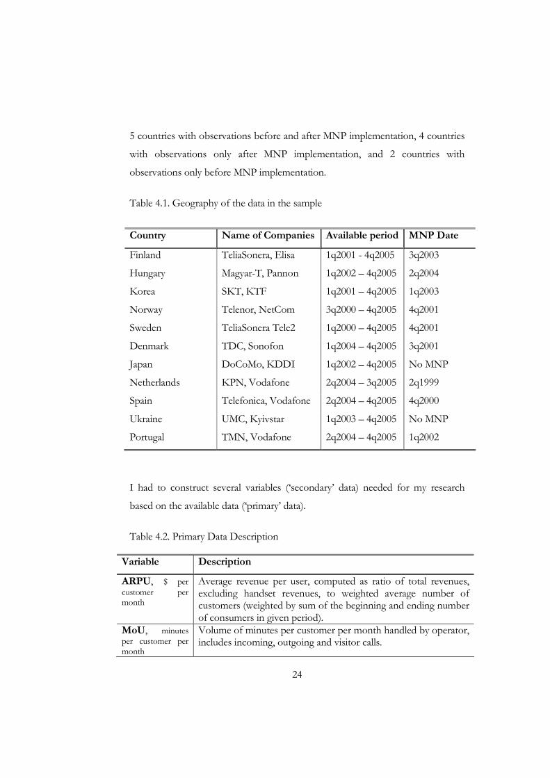
5 countries with observations before and after MNP implementation, 4 countries

with observations only after MNP implementation, and 2 countries with

observations only before MNP implementation.

Table 4.1. Geography of the data in the sample

Country Name of Companies Available period MNP Date

Finland TeliaSonera, Elisa 1q2001 - 4q2005 3q2003

Hungary Magyar-T, Pannon 1q2002 – 4q2005 2q2004

Korea SKT, KTF 1q2001 – 4q2005 1q2003

Norway Telenor, NetCom 3q2000 – 4q2005 4q2001

Sweden TeliaSonera Tele2 1q2000 – 4q2005 4q2001

Denmark TDC, Sonofon 1q2004 – 4q2005 3q2001

Japan DoCoMo, KDDI 1q2002 – 4q2005 No MNP

Netherlands KPN, Vodafone 2q2004 – 3q2005 2q1999

Spain Telefonica, Vodafone 2q2004 – 4q2005 4q2000

Ukraine UMC, Kyivstar 1q2003 – 4q2005 No MNP

Portugal TMN, Vodafone 2q2004 – 4q2005 1q2002

I had to construct several variables (‘secondary’ data) needed for my research

based on the available data (‘primary’ data).

Table 4.2. Primary Data Description

Variable Description

ARPU, $ per customer per month

Average revenue per user, computed as ratio of total revenues, excluding handset revenues, to weighted average number of customers (weighted by sum of the beginning and ending number of consumers in given period).

MoU, minutes per customer per month

Volume of minutes per customer per month handled by operator, includes incoming, outgoing and visitor calls.

25

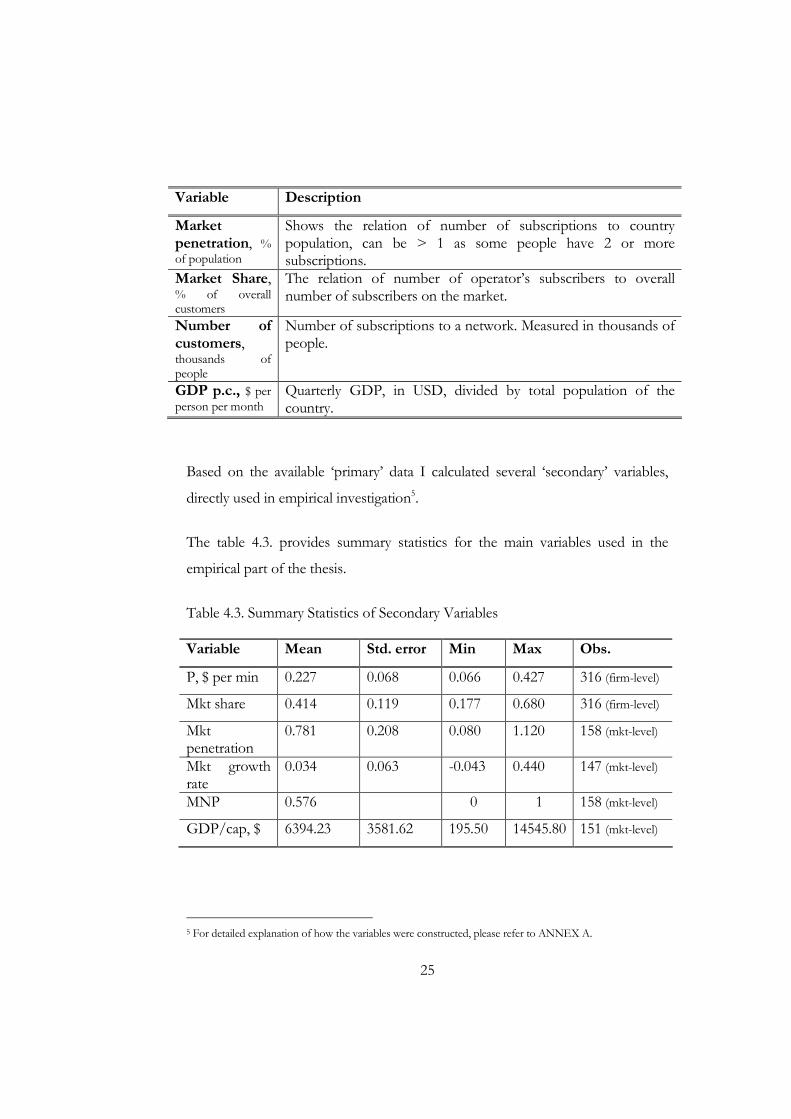
Variable Description

Market penetration, % of population

Shows the relation of number of subscriptions to country population, can be > 1 as some people have 2 or more subscriptions.

Market Share, % of overall customers

The relation of number of operator’s subscribers to overall number of subscribers on the market.

Number of customers, thousands of people

Number of subscriptions to a network. Measured in thousands of people.

GDP p.c., $ per person per month

Quarterly GDP, in USD, divided by total population of the country.

Based on the available ‘primary’ data I calculated several ‘secondary’ variables,

directly used in empirical investigation5.

The table 4.3. provides summary statistics for the main variables used in the

empirical part of the thesis.

Table 4.3. Summary Statistics of Secondary Variables

Variable Mean Std. error Min Max Obs.

P, $ per min 0.227 0.068 0.066 0.427 316 (firm-level)

Mkt share 0.414 0.119 0.177 0.680 316 (firm-level)

Mkt penetration

0.781 0.208 0.080 1.120 158 (mkt-level)

Mkt growth rate

0.034 0.063 -0.043 0.440 147 (mkt-level)

MNP 0.576 0 1 158 (mkt-level)

GDP/cap, $ 6394.23 3581.62 195.50 14545.80 151 (mkt-level)

5 For detailed explanation of how the variables were constructed, please refer to ANNEX A.

26

For empirical estimation I use differences of prices and market shares of two

main competitors on the market (that of larger firm minus that of smaller).

Summary statistics for these differences is presented in table 4.4. below.

Table 4.4. Summary Statistics of Differences of Prices and Market Shares

Variable Mean Std. error Min Max Obs.

tjti pp ,, − -0.011 0.042 -0.148 0.123 151

tjti ,, σσ − 0.203 0.109 -0.088 0.422 151

There are several drawbacks of the dataset used. First, it was impossible to

include each firm from every market, so the dataset has somewhat small size, and

data only on 2 largest firms in every market is included. Almost every mobile

telecommunications market is settled by 3 to 5 mobile carriers. Naturally,

considering only two firms out of 3 or 5 will lead to certain bias, as for example

was shown by Shy (1996) for the Cournot set-up of N identical firms. But on

mobile telecommunications markets firms are very different in terms of size,

mostly because they entered sequentially. Market shares of the remaining players,

besides the two largest, rarely exceeds 25-30% of the market, as presented in table

below.

Table 4.5. Summary Statistics of Joint Shares of not Included Small Players*.

Joint Share of ‘small’ players Country

Min Max Avg

Finland 8.1% 25.2% 16.9% Hungary 12.6% 23.6% 18.9% South Korea 13.9% 26.8% 17.6% Sweden 11.4% 17.4% 14.9% Denmark 21.3% 28.6% 24.4% Japan 20.2% 23.5% 22.5% Netherlands 34.2% 36.8% 35.1% Portugal 19.7% 20.4% 19.9% Spain 17.5% 23.3% 21.0% Ukraine 0.0% 9.0% 3.1% * Summarized across time-period available in the data-set for each country.

27

Among the other countries the ‘outlier’ is Netherlands where 35.1% of market

are not included in the sample. In Netherlands though operate 6 mobile carriers,

that is the unobserved 4 carrier have average share of 8.75% versus 32.4% of

average market of two largest firms in Netherlands. So, it is comparatively small

firms that are not included and I suppose that, under non-cooperative setup6, the

main players concentrate more on competition between each other rather than

with much smaller players. Because of the small size of the unconsidered firms I

expect to have relatively small bias and hope that my results will track closely real-

life situation.

Second, because information on overall number of consumers on the market is

known only approximately - recent entrants with low consumer base and low

revenue almost never disclose their KPIs, – thus data on market penetration and,

more important, on market shares has some measurement problems. In the case

of this data-base measurement error is cushioned by the fact that in some

countries national regulatory authorities provide information on market shares,

and also companies themselves occasionally undertake surveys that allow them to

learn their market shares and disclose more precise estimates.

This data-set is the first firm-level panel to be employed the analysis the effect of

MNP on market competition. So, it provides new opportunities for research and

has the potential to disclose more information on the issue.

6 Padilla (2005) showed that for market with switching costs collusive outcome is hard to achieve and that it is

very unstable.

28

C h a p t e r 5

EMPIRICAL INVESTIGATION

Buehler and Haucap (2004) claimed that empirical estimation of different

effects caused by implementation of MNP is difficult because, firstly, MNP was

introduced only recently and time span observable is very short for empirical

analysis, secondly, very little data on consumer’s switching behavior is publicly

available, thirdly, mobile telecommunications sector develops so dynamically that

it is difficult to isolate effect of MNP empirically.

In my empirical investigation I try to either overcome or avoid these

difficulties. Cross-country firm-level panel data-set provides me with the

sufficient variability, hence mitigating the first difficulty. In my empirical

investigation of the effect of MNP I do not aim to model consumers’ switching

explicitly, thus I do not have to deal with the second difficulty. And finally, in my

regression I include market-specific and time-specific fixed effects which help me

to rule out the effect of technological advancement across different markets and

time periods.

This chapter is structured in the following way. Subsection 5.1 provides the

rationale for the model to be estimated. Subsection 5.2 follows with description

of the empirical methodology applied here. Subsection 5.3 proceeds with

description of the results obtained from the empirical investigation and their

possible value for policy applications.

29

5.1. Rationale for Model Specification

The empirical model that is estimated on the data-set described above has its

root in the results obtained in the mainstream theoretical investigations, described

in literature review part of this thesis.

Now I describe the model, which is estimated in next subsections, in general

terms explaining its connection to the theory. Following the economists which

used the difference between the market shares of the ‘large’ and the ‘small’ firms

as an index of competitiveness (e.g. Shi, 2002; Farrel and Klemperer, 2004). I also

choose difference between market shares of ‘large’ and ‘small’ firms7

( tjtitij ,,, σσσ −= ) as dependent variable for my model. Naturally, we would

like the difference between market shares to decrease, because this means that

market shares of both firms converge. If, after implementation of MNP, market

shares of the firms do not converge, but at the same time average price on the

market decreases, this may lead towards bankruptcy of a smaller firm and hence

towards subsequent deterioration of competition.

Ideally, the general form of the model would be as represented by (5.1.1).

),,,,,( ,1,, tttttijtijtij gpF νψησσ −= (5.1.1)

tij ,σ - the difference between market shares of ‘large’ and ‘small’ firms at t.

1, −tijσ - the difference between market shares of ‘large’ and ‘small’ firms at t-1.

tijp , - the difference between prices charged by ‘large’ and ‘small’ firms at t.

tg - growth rate of the market at t.

tη - market penetration rate – a proxy for future market growth.

tψ - switching costs for an ‘average customer’ on the market at t.

7 Further on the largest firm is denote as ‘Large’ and the second largest as ‘Small’.

30

tv - the interconnection cost between the two networks at t.

Unfortunately, the last two variables are not available for this empirical research.

All the explanatory variables are also picked to utilize the suggestions of the

mainstream literature on MNP, analyzed in the literature review section.

Klemperer (1989) and Beggs and Klemperer (1992) analyzed how difference

between prices charged by ‘large’ and ‘small’ firms ( tijp , ) changes under different

market parameters (growth, size of switching costs) and also explained its

importance for subsequent equilibrium market shares. For example, under high

enough switching costs and slow growth of the market, the ‘large’ firm would

normally charge higher price to ‘rip-off’ its consumers base while ‘small’ would

charge lower price to build-up its customer base. Thus as the result, ceteris

parabis, market shares of the two firms would slowly converge. When market is

growing (or is expected to grow) quickly (large tg , and small tη ), ‘large’ firm

might also try to build-up its customer base, and tijp , will be lower compared to

previous case. Price difference, besides determining equilibrium market shares,

itself is an endogenous variable. Because, the aim of this investigation is analysis

of the changes to market competition which is better reflected by evolution of

market shares, prices are placed among explanatory variables. Next section

includes description of the method I applied to solve this endogeneity problem.

Importance of previous difference between market share, 1, −tijσ , for

predicting next period outcome is discussed by Shi (2002), who argued that

1, −tijσ affects opportunities of customers to receive on-network discounts. As

argued by Shi (2002), Laffont, Rey, and Tirole (1998a,b), ceteris parabis, the firm

with larger market share has advantage in acquiring new customers, as they would

like to benefit more from “on-network” discounts of the ‘large’ firm. These

papers also showed importance of interconnection cost, tv , as degree of market

competition decreases in size of interconnection cost.

31

Switching costs, tψ , are the discussion issue for many authors. Usually, it is

shown that as switching costs decrease, consumers become more willing to

switch. But there were no predictions made considering changes in different

factors’ effects on dynamics of market shares after implementation of MNP. So, I

try to make my own Ex-ante predictions, mostly based on intuition.

It seems that MNP leads to more fierce competition, so possibly than the

effects of the factors determining dynamics of market shares as described above

( tijp , and of tij ,σ ) will increase in magnitude while sign should remain the same.

That is, the lower is the price of ‘Small’ player relatively to that of ‘Large’ one, the

quicker will market shares converge. The larger is present market share of ‘Large’

firm relatively to that of ‘Small’ the slower (quicker) will marker shares converge

(diverge). These effects if not increase, than change anyway, after MNP is

introduced, so it is necessary to know relative importance of each of them for

every particular market, and this investigation aims at doing this.

As main outcome of MNP is a decrease in switching costs (Aoki and

Small (2005)), the natural question is, which factor – tijp , or tij ,σ – will be

decisive for further evolution of market shares and market competition.

Theoretical investigations lead to different conclusions, dependent on

assumptions about model parameters. So, an empirical investigation is needed.

The following investigation estimates effect of the MNP on an ‘average’ market

and determines the condition which is necessary to be satisfied for MNP to lead

towards improvement of competition.

5.2. Estimation Methodology

In this section detailed description of my empirical model is provided along

with analysis of the methods used in its estimation.

32

Based on the general form of my empirical model (5.1.1) below is provided

the model to be estimated on the available cross-country firm-level data-set8:

t

N

nnntttt

tijtijtijtijtij

ucMMgg

MppMM

+++++++

++++++=

∑=

−−

24433

,2,21,11,100,

τβηγηαγα

γασγσαγασ

(5.2.1)

Where tij ,σ , 1, −tijσ , tijp , , tg , tη , are, correspondingly, difference between

market shares of ‘Large’ and ‘Small’ firms at time t, difference between market

shares of ‘Large’ and ‘Small’ firms at time t-1, difference between prices charged

by ‘Large’ and ‘Small’ firm at time t, growth rate of the market at time t, and

market penetration rate at time t.. The model, stated above, as most linear panel

data model, according to Wooldridge, 2002, is most likely a type of unobserved

effects model. So, finally, kc is the unobserved effect, that is unobserved time-

constant variable; and tku , is white noise (or idiosyncratic error).

Switching costs and interconnection costs are not represented in this model

for the reason that they were not available – switching costs is not observable and

hence cannot be reported; interconnection costs are observable and are known to

mobile carriers, but they are not reported regularly and besides are not disclosed

by sufficient number of firms. Possible effects of these two variables on the

explanatory variable will be considered by application of an appropriate

estimation technique. Inclusion of time-specific dummies is necessary for

consideration of technological development that occurs over time.

It is important to mention that price, which is included as an explanatory

variable in the model, is itself a function of market shares of previous period –

firms use price as their actions to maximize their expected flows of profits given

8 Each variable in this regression should also be indexed by country specific index ‘k‘. I do it ‘implicitly’ not to

overload the expression.

33

the observed market parameters. Thus, for model 5.2.1. endogeneity problem

arises. Precisely, the difference between prices is ‘predetermined’:

.0),( , stepcorr stij >⇔≠

Also among the right hand-side variables included is lag of the explained variable

– this also is a source of the endogeneity issue.

Endogeneity necessarily leads to biased estimates, and unreliable predictions.

To deal with the endogeneity problem, I estimate Arellano-Bond linear dynamic

panel-data model. Briefly, benefits of the method is that it corrects for

unobserved effects by taking differences, applies instrumental variable procedure

to correct for endogeneity problem, and also makes it possible to apply robust

estimate of variance-covariance matrix and also to deal with endogeneity at the

same time.

Arellano-Bond Generalized Method of Moments Estimator

The Arellano-Bond GMM estimation procedure goes as follows9. First,

general form of a dynamic panel-data model (similar to that in equation 5.2.1) to

be estimated is represented by expression 5.2.2.

i

itiitit

p

jjtijit

TtNi

wxyay

,...,1,...1

,211

,

==

++++= ∑=

− ενββ (5.2.2)

Where ja are p parameters to be estimated, 1β and 2β are vectors of the

parameters to be estimated.

itx and itw are 11 k× and 21 k× vectors of, correspondingly, strictly exogenous

and predetermined (or endogenous) covariates.

9 For detailed references see Arellano and Bond, 1991.

34

In order to obtain estimates of the parameters ja , 1β and 2β ,

After assuming ρ =2 (2 lags of dependent variable are included in the RHS) lag

differencing the equation 5.2.2. becomes equation 5.2.3, with no random effects

( kc ) left.:

i

itittitiit

TtNi

uxayayy

,...,1,...1

,22,11,

==

∆+∆+∆+∆=∆ −− β (5.2.3)

Then Arellano and Bond provide a procedure to instrument the lags of

explained variable together with the predetermined variables in the model. As

instrumental variables lagged levels of the explained variable are used. Under

assumption of no autocorrelation in idiosyncratic error terms ( itu ) for every i at

t=4 1,iy and 2,iy are valid instruments for the lags of the explained variable.

For t=4 3,iy and 4,iy cannot be used as instruments as they already are in the

model – in the lagged variables on the RHS. Then for every i at t=5 1,iy , 2,iy ,

and 3,iy are the valid instruments, and so on. In such a way matrix of

instruments, iZ , is constructed for every i. :

∆

∆

∆

=

− iTTii

iiii

iii

i

xyy

xyyy

xyy

Z

2,2

6432

532

...00000

000...00

000...000

Λ

ΜΜΜΜΜΟΜΜΜΜ (5.2.4.)

All ix∆ s are strictly exogenous and instrument themselves. Endogenous

(predetermined) variables, iw∆ s, are treated like the lagged dependent variables –

their levels lagged 2 (lagged 1 for predetermined ones) are valid instruments.

35

Matrix iZ , in case of balanced panel data-set, has 1−− ρT rows and

∑−

=

+2

1

T

m

kmρ

columns, where 1k is number of variables in x.

The robust estimator of the variance-covariance matrix, which allows to correct

for heteroscedasticity, is given by :

11

1

*'1

121

1

*111

€ −

=

−

=

′−

= ∑∑ QXZAAAZXQV

N

iii

N

iiir (5.2.5)

Where

= ∑∑

==

N

iii

N

iii XZAZXQ

1

*'1

1

*'1 , ii

N

ii ZHZA ∑

=

=1

'1 , and

][ *'*iii uuEH = , the covariance matrix of differenced idiosyncratic errors.

*iX - vector of all RHS explanatory variables.

The estimation by the Arellano-Bond GMM procedure is based on the

assumption of no serial correlation in the idiosyncratic error, i.e. matrix Hi is

assumed to have zeros outside the main diagonal. In Stata estimation algorithm

automatically provides 2 Arellano-Bond tests – for autocovariance in residuals of

order 1 and for autocovariance in residuals of order 2. According to Arellano and

Bond, 1991, if residuals are autocorrelated of order 1 this leads to inefficiency of

the estimates. But is autocovariance of order 2 (or higher) is present, the estimate

will be biased.

The next subsection provides description and verification of the estimation

results.

36

5.3. Interpretation of Estimation Results

Along way of estimating the Arellano-Bond GMM model, I also estimated

pooled OLS model (Model [1]), fixed-effect model (Model [2]), random-effect

model with AR(1) residuals (Model [3]), and 2 Stages Least-Squares model

(Model [4]). This allows me to better learn properties of the data-set at hand and

compare the estimation results to the estimation results of the ultimate Arellano-

Bond GMM model (Model [5]). All the estimates are placed in table 5.3.2 below.

Before estimating the model, the theoretical predictions about the signs of

coefficients near the factors predicting market share evolution is placed in table

5.3.1. My own ex-ante expectations about signs of the change of the coefficients

near the factors are also placed in table.

Table 5.3.1. Expectations of Signs of Explanatory Variables

Regressor 1, −tijσ 1, −tijtM σ * tijp , tijMp , *

Expected Sign + + - - Regressor

tg tMg * tη tMη *

Expected Sign + + + + * - my own expectations.

To estimate Model [2] I choosed fixed-effect model, based on Hausman test.

Also, for estimation Model [3] random-effect model was chosen based on

Hausman test. Also after estimation of Model [3] Breusch-Pagan tests for random

effects and founds no evidence of those.

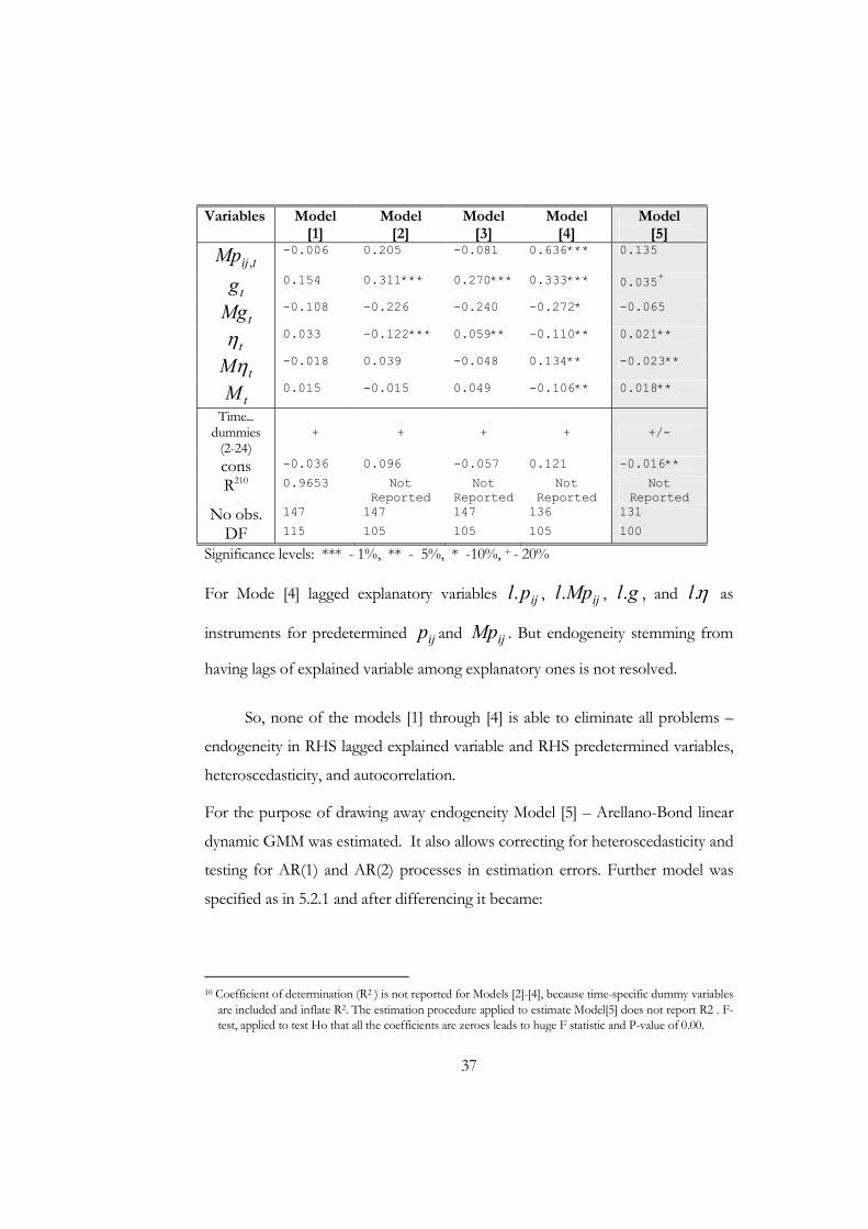
Table 5.3.2. Estimation Results for Main Specifications of the Model

Variables Model [1]

Model [2]

Model [3]

Model [4]

Model [5]

1, −tijσ 0.983*** 0.844*** 0.982*** 0.766*** 0.793***

1, −tijtM σ

-0.023 -0.048 -0.052 0.123 -0.041**

tijp , -0.004 -0.098 0.029 -0.340 -0.098

37

Variables Model [1]

Model [2]

Model [3]

Model [4]

Model [5]

tijMp , -0.006 0.205 -0.081 0.636*** 0.135

tg 0.154 0.311*** 0.270*** 0.333*** 0.035+

tMg -0.108 -0.226 -0.240 -0.272* -0.065

tη 0.033 -0.122*** 0.059** -0.110** 0.021**

tMη -0.018 0.039 -0.048 0.134** -0.023**

tM 0.015 -0.015 0.049 -0.106** 0.018**

Time_ dummies (2-24)

+ + + + +/-

cons -0.036 0.096 -0.057 0.121 -0.016**

R210 0.9653 Not Reported

Not Reported

Not Reported

Not Reported

No obs. 147 147 147 136 131

DF 115 105 105 105 100

Significance levels: *** - 1%, ** - 5%, * -10%, + - 20%

For Mode [4] lagged explanatory variables ijpl. , ijMpl. , gl. , and η.l as

instruments for predetermined ijp and ijMp . But endogeneity stemming from

having lags of explained variable among explanatory ones is not resolved.

So, none of the models [1] through [4] is able to eliminate all problems –

endogeneity in RHS lagged explained variable and RHS predetermined variables,

heteroscedasticity, and autocorrelation.

For the purpose of drawing away endogeneity Model [5] – Arellano-Bond linear

dynamic GMM was estimated. It also allows correcting for heteroscedasticity and

testing for AR(1) and AR(2) processes in estimation errors. Further model was

specified as in 5.2.1 and after differencing it became:

10 Coefficient of determination (R2 ) is not reported for Models [2]-[4], because time-specific dummy variables

are included and inflate R2. The estimation procedure applied to estimate Model[5] does not report R2 . F-

test, applied to test Ho that all the coefficients are zeroes leads to huge F statistic and P-value of 0.00.

38

t

T

mtmmtttt

tijtijtijtijtij

ulMaMgga

MppaMa

+∆+∆+∆+∆+∆+

+∆+∆+∆+∆=∆

∑=

−−

2,4433

,2,21,11,1,

τηγηγ

γσγσσ

(5.3.1.)

Where the usual notation is used – tij,σ∆ and 1, −∆ tijσ - differenced difference

between market shares and lagged differenced difference between market shares.

tijp ,∆ - differenced difference of prices, tg∆ and tη∆ - are differences of

growth rate and penetration rate of the market.

The Arellano-Bond procedure instruments such variables as

1, −∆ tijσ , )( 1, −∆ tijMσ , tijp ,∆ , and )( ,tijMp∆ with, firstly, lags of levels of

ijσ , secondly, first and second lags of themselves.

The signs of the coefficients near the factors explaining the evolution of market

shares of the specification Model [5] appeared to be entirely in line with the

mainstream theory. But my expectations about the effect of MNP on magnitude

of the explaining factors turned wrong. Let’s now consider the results in more

detail and analyze the findings.

Positive and strongly significant coefficient of 1, −tijσ shows that the firm with

larger market share will manage to keep about 79% of the difference between

market shares in the next period as well. But introduction of MNP decreases the

capacity of ‘Large’ firm to maintain its high market share, as coefficient near

1, −tijtM σ is negative and significant.

As predicted by the theory, tijp , is negative. That is, the stronger Small firm

undercuts Large one, the faster market shares converge. The other result is that

39

tijMp , is positive, and ‘marginally’ significant – at 15% s. l., meaning that

marginal effect from efforts of Small firm to undercut its Large competitor

decreases under implemented MNP.

Positive and significant coefficient near tg supports the theoretical suggestions

stated above. This result could be interpreted that probability that of incumbent

firm to engage in penetration pricing is increasing in market growth rate. MNP

seem to have decreasing effect on the probability of incumbent operator to

engage in penetration pricing, as coefficient near tMg is negative.

Penetration rate tη , is used in the empirical model as an ‘inverted’ proxy for

future expected market growth, should have and actually has properties similar to

the previous factor. Penetration rate is positive and significant, but MNP also

decreases it.

The dummy for MNP ( tM ) is positive and significant. But, according to

methodology there should not be an intercept in the model after differencing. But

still we could try to interpret this variable. – If there are some other mechanisms,

not included in the empirical model being estimated, for example, decreased

degree of information available to consumers, MNP leads towards decrease in

competition through those mechanisms as marginal effect of the dummy alone is

towards divergence of market shares of the firms.

So the empirical results support what most theoretical works would predict, and

it would also be interesting to derive some ‘requirements’ for the market

parameters (such as penetration rate and growth rate) that would guarantee

positive outcome of MNP implementation for market competition. Some

algebraic manipulations below result in a simple rule for policy-makers. Besides,

40

based on the estimated coefficients of Model [5] some simulations are provided

on figure 5.3.1. to better illustrate the meaning of the equation rule 5.3.5.

For MNP implementation to have positive outcome, in terms of improving

competition, means that the difference between the market shares of the firms

should decrease more than otherwise. That is, MNP portability should be

implemented if and only if:

MNPNOtij

MNPtij

_,, σσ ≤ , (5.3.2)

or after substituting from the equation (5.3.1)11:

tttijtijt

ttijtij

agapaaaba

gbapbababa

ηση

σ

43,21,1044

33,221,1100

)(

)()()()(

++++≤++

++++++++

−

− (5.3.3)

Where 0b , 1b , 2b , 3b , 4b are the estimated (in Model [5]) intercept coefficients of

the interaction terms of MNP dummy with other variables. Variables are not

differenced now, because, according to Wooldridge, 2002, differencing was

needed to only for estimation purposes – to get rid of unobservable fixed effects,

but for interpretation original model should be used.

After simple arithmetic transformations 5.3.3 becomes:

1

431,20

1,b

bgbpbb tttij

tij

ησ

+++−≤ −

− (5.3.4)

If updated 1 period ahead (5.3.3) becomes:

11 For the LHS value coefficients near explanatory variables are summed with the correspondent coefficients

near explanatory variables interacted with the dummy for MNP. For the RHS value only coefficients near

explanatory variables are used.

41

1

1413,20

,

)()(

b

EbgEbpbb tttij

tij

++ ++∆+−≤

ησ (5.3.5)

Expression (5.3.5.) gives the condition for testing possible effect of MNP for

market competition. As 5.3.4 is derived from inequality 5.3.2., it tells that for

MNP to have positive outcome it is necessary that present difference between

market shares of the two firms to be smaller than minus the expression of today’s

price difference, expected future growth and penetration rates.

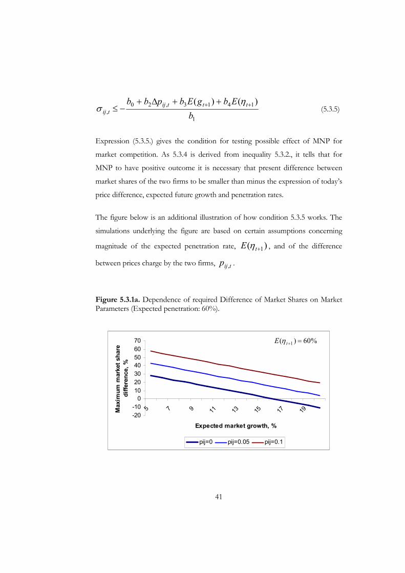
The figure below is an additional illustration of how condition 5.3.5 works. The

simulations underlying the figure are based on certain assumptions concerning

magnitude of the expected penetration rate, )( 1+tE η , and of the difference

between prices charge by the two firms, tijp , .

Figure 5.3.1a. Dependence of required Difference of Market Shares on Market Parameters (Expected penetration: 60%).

-20

-10

0

10

20

30

40

50

60

70

5 7 9 11 13 15 17 19

Expected market growth, %

Maximum market share

difference, %

pij=0 pij=0.05 pij=0.1

%60)( 1 =+tE η

42

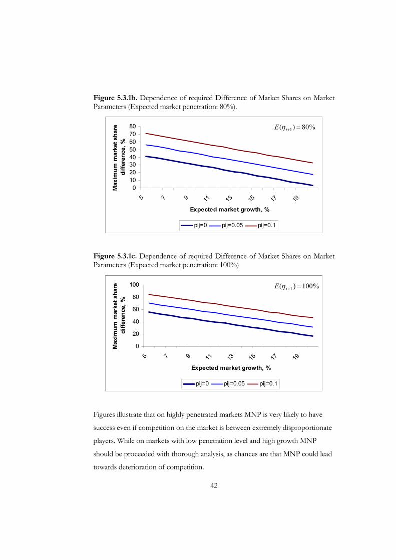
Figure 5.3.1b. Dependence of required Difference of Market Shares on Market Parameters (Expected market penetration: 80%).

0

10

20

30

40

50

60

70

80

5 7 9 11 13 15 17 19

Expected market growth, %

Maximum market share

difference, %

pij=0 pij=0.05 pij=0.1

Figure 5.3.1c. Dependence of required Difference of Market Shares on Market Parameters (Expected market penetration: 100%)

0

20

40

60

80

100

5 7 9 11 13 15 17 19

Expected market growth, %

Maximum market share

difference, %

pij=0 pij=0.05 pij=0.1

Figures illustrate that on highly penetrated markets MNP is very likely to have

success even if competition on the market is between extremely disproportionate

players. While on markets with low penetration level and high growth MNP

should be proceeded with thorough analysis, as chances are that MNP could lead

towards deterioration of competition.

%80)( 1 =+tE η

%100)( 1 =+tE η

43

C h a p t e r 6

CONCLUSION

Though MNP is usually considered as a technology that fosters competition on a

mobile telecommunications market, it is mot always the case. Though in Sweden

and Finland it lead to increased competition, as measured by faster convergence

of market shares, in such countries as Hong Kong, Korea it caused inverse

effect – market shares diverged. Therefore it looks necessary to verify whether

MNP will have competition-improving or competition-deteriorating effect

beforehand.

In this thesis I developed model of competition between two mobile carriers,

where consumers have switching costs, and there are interconnection costs on

the market. It seams that no closed solution is available for the model, but in

series of simulation I found that such market variables as growth rate,

interconnection costs play important role for predetermining the effect of MNP.

Also an empirical investigation was undertaken. The dynamic panel-data model

was estimated by Arellano-Bond GMM estimator. The results supported

suggestions of previous theoretical works and findings of the model developed in

this thesis.

I believe, that MNP is still an issue to be researched much. And ideas and

findings of this paper could stimulate further research and might help avoid

negative consequences of MNP in some countries.

44

BIBLIOGRAPHY

Aoki R., Small J. (2005), “The Economics of Number Portability: Switching Costs and Two-Part Tariffs.” Working Paper, Institute of Economic Research, Hitotsubashi University.

Arellano M., Bond S. (1991), “Some Tests of Specification for Panel Data: Monte Carlo Evidence and an Application to Employment Equations,” The Review of Economic Studies Vol. 58. Pp 277-297.

Armstrong M. (1998), “Network Interconnection in Telecommunications.” The Economic Journal, Vol. 108, No 488.

Attenborough N., Sandbach J., Saadat U., Siolis G., Cartwright M., Dunkley S. (1998) “Feasibility Study and Cost Benefit Analysis of Number Portability for Mobile Services in Hong Kong.” Final Report for OFTA prepared by NERA and Smith System Engineering.

Beggs A., Klemperer P. (1992), “Multi-Period Competition With Switching Costs,” Econometrica, Vol. 60, No. 3, 651-666

Bezzina J., Penard T. Dynamic Competition in the Mobile Market, Subsidies and collusion. University of Rennes Working Paper, 2000.

Buehler S., Haucap J. (2004)“Mobile Number Portability.” Working paper, University of Zurich, Socioeconomic Institute.

Campo-Rembado M., Sundararajan A. (2004), “Competition in Wireless telecommunications,” Working Paper, Leonard N. Stern School of Business, New York University

Capuano C. (2002), “Intertemporal Complementarity and Self-Competition Between Charge Profiles in Mobil Communication Services: a Case of Endogenous Most Favoured Customer Condition,” Working Paper, Universita degli Studi di Napoli Federico II

Carlsson F. (2004), “Airline choice, switching costs and frequent flyer program,” Working Paper № 123, Gothenburg University

Chakravarty S. (2005), “Determinants of Cellular Competition in Asia,” Working Paper, Indian Institute of Management, Ahmedabad.

Corrocher N., Zirulia L. (2005), “Switching Costs, Consumer’s Heterogeneity and Price Discrimination in the Mobile Communications Industry,” Working Paper, CESPRI, Bocconi University, Milan

41

Farrell, J. and Shapiro, C. (1988), “Optimal Contracts with Lock-In,” American Economic Review, No. 79(1), 51-68

Farrell J., Klemperer P. (2004), “Coordination and Lock-In: Competition with Switching Costs and Network Effects,” Working Paper, Nuffield College, Oxford University

Fudenberg D., Tirole J. (1998), “Game Theory.” The MIT Press. Cambridge, Massachusetts. London, England. pp. 35-35.

Gabrielsen T., Vagstad S. (2002), “Markets With Consumer Switching Costs and Non-Linear Pricing,” Working Paper, University of Bergen

Grzybovski L. (2005), “Estimating Switching Costs in Mobile Telephony in UK,” Working Paper, Center for Information and Network Economics, University of Munich.

Kim H., Kwon N. (2003), “The Advantage of Network Size in Acquiring New Subscribers: a Conditional Logit Analysis of the Korean Mobile Telephony Market,” Information Economics and Policy, No 15, 17-33

Klemperer P., (1987a), “The Competitiveness of Markets With Switching Costs,” The RAND Journal of Economics, Vol. 18, pp 138-150.

Klemperer P., (1987b), “Entry Deterrence in Markets with Consumer Switching Costs,” The Economic Journal, No.97, 99-117

Klemperer P., (1988), “Welfare Effects of Entry Into Markets With Switching Costs,” The Journal of Industrial Economics, Vol.32, No2, pp. 159-165.

Klemperer P. (1989), “Price Wars Caused by Switching Costs,” Review of Economic Studies (1989) No. 56, 405-420

Klemperer P. (1995), “Competition when Consumers have Switching Costs: An Overview with Application to Industrial Organization, Macroeconomics, and International Trade,” The Review of Economic Studies, Vol. 62, No 4, 515-539

Padilla A., McSorley C., Alejandro R,Watson N., Williams M. (2003), “Switching Costs: Annex B – Review of empirical methods for identifying and measuring Switching Costs,” Report prepared for the Office of Fair Trading and the Department of Trade and Industry by National Economic Research Associates

Kim J. (2005), “The Effect of mobile Number Portability on Switching Costs in the Telecommunication Industry,” Working Paper, The University of Wisconsin-Madison

Kim M., Kliger D., Vale B. (2003), “Estimating Switching Costs: the Case of Banking,” Journal of Financial Intermediation No. 12 (2003), 25-56

42

Laffont J., Rey P., Tirole J. (1998a) “Network Competition: I. Overview and Nondiscriminatory Pricing.” The RAND Journal of Economics, vol. 29, No 1. pp. 1-37.

Laffont J., Rey P., Tirole J. (1998b) “Network Competition: II.Price Discrimination.” The RAND Journal of Economics, vol. 29, No 1. pp. 38-56.

Padilla A. J. (1995), “Revisiting Dynamic Duopoly with Consumer Switching Costs,” Journal of Economic Theory, No. 67(2), 520-530

Shi M., Chiang J., Rhee B. (2002), “Price Competition with Reduced Consumer Switching Costs: The Case of “Wireless Number Portability” in the Cellular Industry.” Working Paper, The University of Toronto.

Shy O. (2002), “A quick-and-easy method for estimating switching costs,” International Journal of Industrial Organizations, vol. 20, 71-87

Shy O. (1996), “Industrial Organizations: Theory and Applications,” The MIT Press. Cambridge, Massachusetts. London, England. Pp. 101-103

Vives X. (2005), “Complementarities and Games: New Developments,” Journal of Economic Literature 43, 437-479

Wooldridge J. (2002), “Econometric Analysis of Cross-Section and Panel Data.” The MIT Press. Cambridge, Massachusetts. London, England. Pp. 249-297.

43

ANNEX A: Proof of Proposition 1.

After substitution of (3.3.1.a) and (3.3.1.b) into (3.3.2.) and reshuffling it is possible to

obtain:

AABBBBAABBBAAA XSnvvvvvvn ττσ 2)()( +−−−=−−+ [1]

After substitution of (3.3.1.a) and (3.3.1.b) into (3.3.3.) and into (3.3.4) and reshuffling ,

we by the same token obtain:

BABBBBAABBBAAA XSnvvvvvvn ττσ 2)()( ++−−=−−+ [2]

Xnvvvvvvn ABBBBAABBBAAA ττσ 2)()( +−−=−−+ [3]

Then from pair-wise equating the expressions [1], [2], and [3] we obtain three groups of

conditions, which will be substituted into the expression for market share of A ( Aσ ):

(A)

τ

τ

2

SXX

SXX

A

AB

−=

−=

(B)

τ

τ

2

SXX

SXX

B

BA

+=

+=

(C)

τ

τ

2

2

SXX

SXX

B

A

−=

+=

Now, it is possible to transform the expression for c(3.5.5.) in the following way:

+

+

+

+

+

=NK

NX

NK

KX

NK

KX B

BA

AA

θθσ [4]

Then, to calculate the indifferent consumer position, we do the following: for XA we

substitute conditions (A) into Aσ and into [1]; for XB we substitute conditions (B) into Aσ

and into [2]; for X we substitute conditions (C) into Aσ and into [3]. After that the

proportions (3.3.6.) are calculated.

44

ANNEX B. Proof of Proposition 2

)])(1()([)( AABAAAAAAAAA mcpnqcpnNK −−+−+= σσσπ

s.t. AABAAAA wvnvn =−+ )1( σσ

Let’s set up the L’Agrangian and find the first-order conditions:

))1((

)])(1()([)(

ABAAAAA

AABAAAAAAAA

vnvnw

mcpnqcpnNK

σσλ

σσσξ

−+−−

−−−+−+=

FOC:

(1) 0)()()( '' =+⋅−++⋅+=∂∂

AAAAAAAAAAA

AA

vqcpNKqNKp

λσσξ

(2) 0)()()( '' =+⋅−++⋅+=∂∂

ABABAABAABA

AB

vqmcpNKqNKp

λσσξ

Express λ to RHS in each of the two equations and combine them. Then as

Bqq ABAA −== '',

)()( AABAAAAAAB mcpqcpq −=− ,

After substituting the expressions for AAq and ABq , and few arithmetic transformation,

We obtain the target expression:

A

A

A

AAAAB

cBA

mAc

cBA

mcBApp

⋅−−

+⋅−

⋅⋅−=

)1(, or

AAAAAB kkpp 01 += , where

A

AA

A

AA

cBA

mAck

cBA

mcBAk

⋅−−

=⋅−

⋅⋅−=

)1(, 01 .

By symmetry, for firm B we obtain:

B

B

B

BBBBA

cBA

mAc

cBA

mcBApp

⋅−−

+⋅−

⋅⋅−=

)1(, or

BBBBBA kkpp 01 += , where

B

BB

B

BB

cBA

mAck

cBA

mcBAk

⋅−−

=⋅−

⋅⋅−=

)1(, 01 .

QED.

45

ANNEX C: Algorithm for Calculating the Nash Equilibrium

This algorithm is developed independently, and so far it has not been tasted yet for

precision of results. But because of the methods it relies on, I believe that results are

reasonably precise.

Obtaining Nash Equilibrium:

1) Divide range of price by B into 200 small pieces and find length of one.

Then by iterating Bp in bounds determined by the value of marginal costs and the

upper bound as defined after (3.2.3), obtain values of Ap (also bounded) which

maximize profit of firm A for every value of Bp .

2) Estimate the optimal response function of firm A, by applying Chebyshev’s

polynomial for regressing Ap on Bp . Chebyshev’s polynomial is constructed in the

way to minimize collinearity among regressors. Thus the coefficients of determination

obtained were rather high.

3) and 4) Do the procedures described in 2) and 3) for firm B.

4) Solve the system of nonlinear equations:

=

=

)(

)(

AABBB

BBAAA

pRp

pRp.

Chebyshev’s Polinomial

))(coscos()(),(...)()( 10 XnXTXTXTXF nn

−⋅=++≈

46

ANNEX D: Evolution of Market Shares under MNP (Decreased Switching Costs)

Assumptions: %25%75 ,, == tjti σσ , %30==t

tt

K

Ng , ;2=tM

Evolution of Market Shares under MNP

0

0.1

0.2

0.3

0.4

0.5

0.6

0.7

3 2.75 2.5 2.25 2

Switching Costs

Market Shares

Large

Small

Assumptions: %25%75 ,, == tjti σσ , %5==t

tt

K

Ng , ;2=tM

Evolution of Market Shares under MNP

0

0.1

0.2

0.3

0.4

0.5

0.6

0.7

0.8

3 2.75 2.5 2.25 2

Switching Costs

Market Shares

Large

Small

Assumptions: %25%75 ,, == tjti σσ , %50==t

tt

K

Ng , ;2=tM

Evolution of Market Shares under MNP

0

0.1

0.2

0.3

0.4

0.5

0.6

0.7

3 2.75 2.5 2.25 2

Switching Costs

Market Shares

Large

Small

47

ANNEX E: Evolution of Market Shares under MNP (Decreased Switching Costs)

Assumptions: %25%75 ,, == tjti σσ , %5==t

tt

K

Ng , ;2=tM

Evolution of Market Shares under MNP

0

0.1

0.2

0.3

0.4

0.5

0.6

0.7

0.8

3 2.75 2.5 2.25 2

Switching Costs

Market Shares

Large

Small

Assumptions: %25%75 ,, == tjti σσ , %30==t

tt

K

Ng , ;75.2=tM

Evolution of Market Shares under MNP

0

0.1

0.2

0.3

0.4

0.5

0.6

0.7

0.8

3 2.75 2.5 2.25 2

Switching Costs

Market Shares

Large

Small

Assumptions: %25%75 ,, == tjti σσ , %30==t

tt

K

Ng , ;5.3=tM

Evolution of Market Shares under MNP

0

0.2

0.4

0.6

0.8

1

3 2.75 2.5 2.25 2

Switching Costs

Market Shares

Large

Small

48

ANNEX F: Evolution of Per-Minute Prices under MNP (Decreased Switching Costs)

Assumptions: %25%75 ,, == tjti σσ , %5==t

tt

K

Ng , ;2=tM

Evolution of Prices under MNP

0

0.05

0.1

0.15

0.2

0.25

3 2.75 2.5 2.25 2

Switching Costs

Per-Minute Prices

Large

Small

Assumptions: %25%75 ,, == tjti σσ , %30==t

tt

K

Ng , ;2=tM

Evolution of Prices under MNP

0

0.05

0.1

0.15

0.2

0.25

3 2.75 2.5 2.25 2

Switching Costs

Per-Minute Prices

Large

Small

Assumptions: %25%75 ,, == tjti σσ , %50==t

tt

K

Ng , ;2=tM

Evolution of Prices under MNP

0

0.05

0.1

0.15

0.2

0.25

3 2.75 2.5 2.25 2

Switching Costs

Per-Minute Prices

Large

Small

49

ANNEX G: Evolution of Per-Minute Prices under MNP (Decreased Switching Costs)

Assumptions: %25%75 ,, == tjti σσ , %5==t

tt

K

Ng , ;2=tM

Evolution of Prices under MNP

0

0.05

0.1

0.15

0.2

0.25

3 2.75 2.5 2.25 2

Switching Costs

Per-Minute Prices

Large

Small

Assumptions: %25%75 ,, == tjti σσ , %5==t

tt

K

Ng , ;75.2=tM

Evolution of Prices under MNP

0

0.05

0.1

0.15

0.2

3 2.75 2.5 2.25 2

Switching Costs

Per-Minute Prices

Large

Small

Assumptions: %25%75 ,, == tjti σσ , %5==t

tt

K

Ng , ;5.3=tM

Evolution of Prices under MNP

0

0.02

0.04

0.06

0.08

0.1

0.12

0.14

0.16

3 2.75 2.5 2.25 2

Switching Costs

Per-Minute Prices

Large

Small

50

ANNEX H: CONSTRUCTION OF VARIABLES FOR ESTIMATION

I constructed six new variables ( itp , tijp , , tij ,σ , itg , itη , tM ) from the available data, as

represented by Table 4.2. The ways to construct the variables are provided below.

(1). Prices:

it

itit

MoU

ARPUp = ,

(2). Difference between prices of two mobile carriers: tjtitij ppp ,,, −= ,

i denotes carrier with the largest market share and j – the one with the second largest market

share.

In same way, difference between market shares of the two mobile carriers is:

(3). tjtitij ,,, σσσ −=

Same as above, i denotes carrier with the largest market share and j – the one with the second

largest market share.

(4). Growth rate

1−

=t

t

tcustomersmarketTotal

customersmarketTotalg ;

(5). Market penetration12 -

t

N

it

tpop

consumers∑== 1η ;

it

itN

it

consumersconsumers

σ=∑

=1

Market penetration shows fraction of total number of subscriptions to mobile services to total

population of the country.

(6). Dummy for MNP ( tM ) was constructed in a way that it equals 1 in the periods of MNP

implementation and afterwards and equals 0 in periods prior to MNP implementation.

12 When market penetration was not provided in KPIs, I constructed it based on other information, as shown in formula (5)

above.

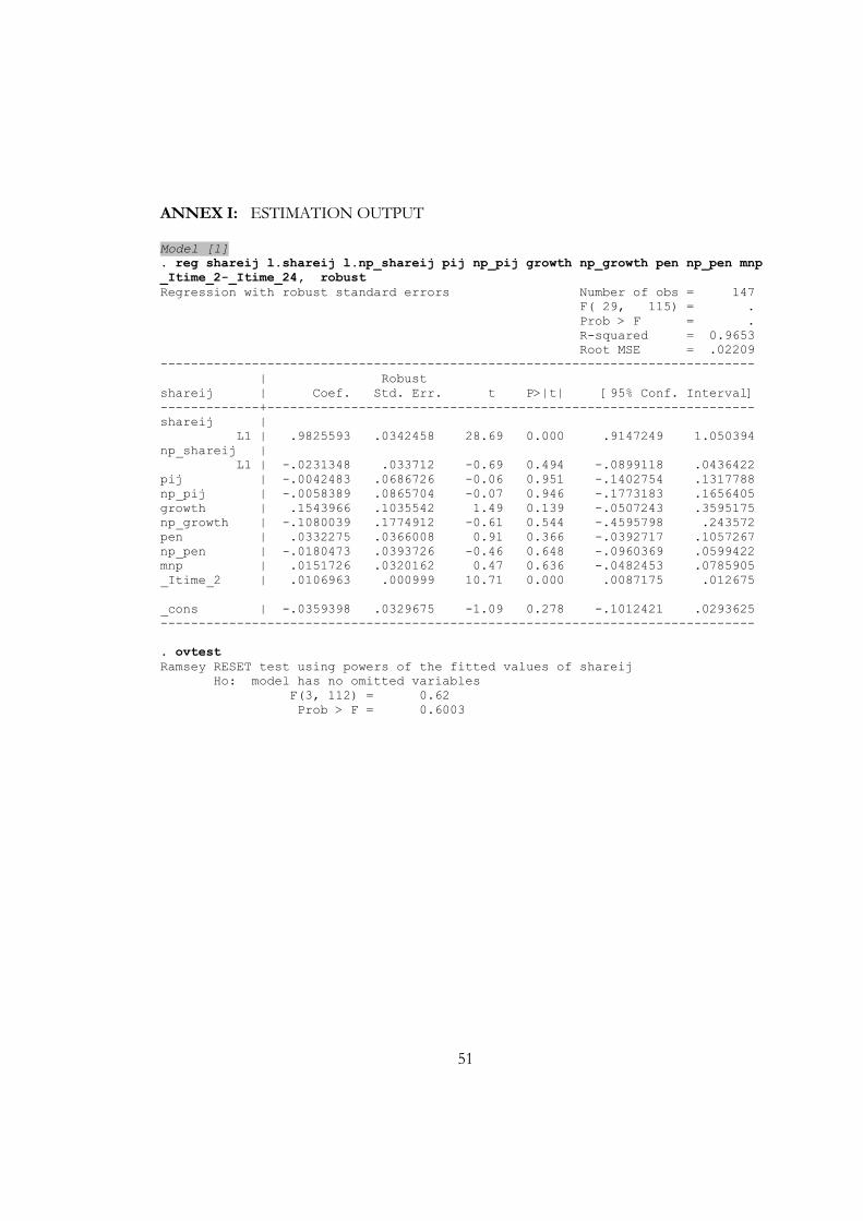
51

ANNEX I: ESTIMATION OUTPUT Model [1]

. reg shareij l.shareij l.np_shareij pij np_pij growth np_growth pen np_pen mnp _Itime_2-_Itime_24, robust Regression with robust standard errors Number of obs = 147 F( 29, 115) = . Prob > F = . R-squared = 0.9653 Root MSE = .02209 ------------------------------------------------------------------------------ | Robust shareij | Coef. Std. Err. t P>|t| [95% Conf. Interval] -------------+---------------------------------------------------------------- shareij | L1 | .9825593 .0342458 28.69 0.000 .9147249 1.050394 np_shareij | L1 | -.0231348 .033712 -0.69 0.494 -.0899118 .0436422 pij | -.0042483 .0686726 -0.06 0.951 -.1402754 .1317788 np_pij | -.0058389 .0865704 -0.07 0.946 -.1773183 .1656405 growth | .1543966 .1035542 1.49 0.139 -.0507243 .3595175 np_growth | -.1080039 .1774912 -0.61 0.544 -.4595798 .243572 pen | .0332275 .0366008 0.91 0.366 -.0392717 .1057267 np_pen | -.0180473 .0393726 -0.46 0.648 -.0960369 .0599422 mnp | .0151726 .0320162 0.47 0.636 -.0482453 .0785905 _Itime_2 | .0106963 .000999 10.71 0.000 .0087175 .012675 _cons | -.0359398 .0329675 -1.09 0.278 -.1012421 .0293625 ------------------------------------------------------------------------------ . ovtest Ramsey RESET test using powers of the fitted values of shareij Ho: model has no omitted variables F(3, 112) = 0.62 Prob > F = 0.6003

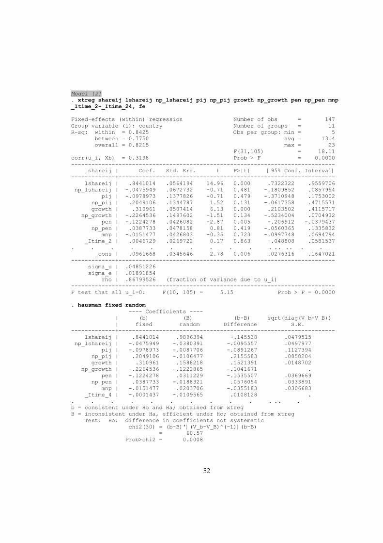
52

Model [2]

. xtreg shareij lshareij np_lshareij pij np_pij growth np_growth pen np_pen mnp _Itime_2-_Itime_24, fe Fixed-effects (within) regression Number of obs = 147 Group variable (i): country Number of groups = 11 R-sq: within = 0.8425 Obs per group: min = 5 between = 0.7750 avg = 13.4 overall = 0.8215 max = 23 F(31,105) = 18.11 corr(u_i, Xb) = 0.3198 Prob > F = 0.0000 ------------------------------------------------------------------------------ shareij | Coef. Std. Err. t P>|t| [95% Conf. Interval] -------------+---------------------------------------------------------------- lshareij | .8441014 .0564194 14.96 0.000 .7322322 .9559706 np_lshareij | -.0475949 .0672732 -0.71 0.481 -.1809852 .0857954 pij | -.0978973 .1377826 -0.71 0.479 -.3710948 .1753002 np_pij | .2049106 .1344787 1.52 0.131 -.0617358 .4715571 growth | .310961 .0507414 6.13 0.000 .2103502 .4115717 np_growth | -.2264536 .1497602 -1.51 0.134 -.5234004 .0704932 pen | -.1224278 .0426082 -2.87 0.005 -.206912 -.0379437 np_pen | .0387733 .0478158 0.81 0.419 -.0560365 .1335832 mnp | -.0151477 .0426803 -0.35 0.723 -.0997748 .0694794 _Itime_2 | .0046729 .0269722 0.17 0.863 -.048808 .0581537 . . . . . . . . . . . . . . . . . _cons | .0961668 .0345646 2.78 0.006 .0276316 .1647021 -------------+---------------------------------------------------------------- sigma_u | .04851226 sigma_e | .01891854 rho | .86799526 (fraction of variance due to u_i) ------------------------------------------------------------------------------ F test that all u_i=0: F(10, 105) = 5.15 Prob > F = 0.0000 . hausman fixed random ---- Coefficients ---- | (b) (B) (b-B) sqrt(diag(V_b-V_B)) | fixed random Difference S.E. -------------+---------------------------------------------------------------- lshareij | .8441014 .9896394 -.145538 .0479515 np_lshareij | -.0475949 -.0380391 -.0095557 .0497977 pij | -.0978973 -.0087706 -.0891267 .1127394 np_pij | .2049106 -.0106477 .2155583 .0858204 growth | .310961 .1588218 .1521391 .0148702 np_growth | -.2264536 -.1222865 -.1041671 . pen | -.1224278 .0311229 -.1535507 .0369669 np_pen | .0387733 -.0188321 .0576054 .0333891 mnp | -.0151477 .0203706 -.0355183 .0306683 _Itime_4 | -.0001437 -.0109565 .0108128 . . . . . . . . . . . . . . . b = consistent under Ho and Ha; obtained from xtreg B = inconsistent under Ha, efficient under Ho; obtained from xtreg Test: Ho: difference in coefficients not systematic chi2(30) = (b-B)'[(V_b-V_B)^(-1)](b-B) = 60.57 Prob>chi2 = 0.0008

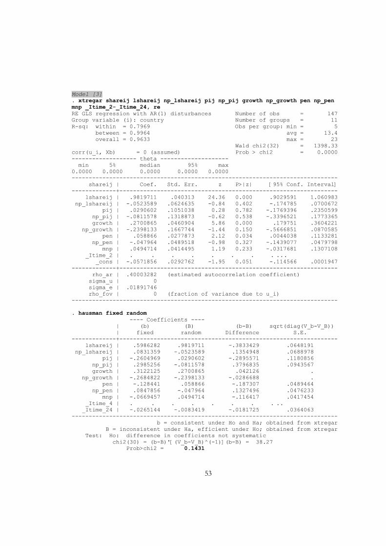
53

Model [3]

. xtregar shareij lshareij np_lshareij pij np_pij growth np_growth pen np_pen mnp _Itime_2-_Itime_24, re RE GLS regression with AR(1) disturbances Number of obs = 147 Group variable (i): country Number of groups = 11 R-sq: within = 0.7969 Obs per group: min = 5 between = 0.9964 avg = 13.4 overall = 0.9633 max = 23 Wald chi2(32) = 1398.33 corr(u_i, Xb) = 0 (assumed) Prob > chi2 = 0.0000 ------------------- theta -------------------- min 5% median 95% max 0.0000 0.0000 0.0000 0.0000 0.0000 ------------------------------------------------------------------------------ shareij | Coef. Std. Err. z P>|z| [95% Conf. Interval] -------------+---------------------------------------------------------------- lshareij | .9819711 .040313 24.36 0.000 .9029591 1.060983 np_lshareij | -.0523589 .0624635 -0.84 0.402 -.174785 .0700672 pij | .0290602 .1051038 0.28 0.782 -.1769396 .2350599 np_pij | -.0811578 .1318873 -0.62 0.538 -.3396521 .1773365 growth | .2700865 .0460904 5.86 0.000 .179751 .3604221 np_growth | -.2398133 .1667744 -1.44 0.150 -.5666851 .0870585 pen | .058866 .0277873 2.12 0.034 .0044038 .1133281 np_pen | -.047964 .0489518 -0.98 0.327 -.1439077 .0479798 mnp | .0494714 .0414495 1.19 0.233 -.0317681 .1307108 _Itime_2 | . . . . . . . . . . . _cons | -.0571856 .0292762 -1.95 0.051 -.114566 .0001947 -------------+---------------------------------------------------------------- rho_ar | .40003282 (estimated autocorrelation coefficient) sigma_u | 0 sigma_e | .01891746 rho_fov | 0 (fraction of variance due to u_i) ------------------------------------------------------------------------------ . hausman fixed random ---- Coefficients ---- | (b) (B) (b-B) sqrt(diag(V_b-V_B)) | fixed random Difference S.E. -------------+---------------------------------------------------------------- lshareij | .5986282 .9819711 -.3833429 .0648191 np_lshareij | .0831359 -.0523589 .1354948 .0688978 pij | -.2604969 .0290602 -.2895571 .1180856 np_pij | .2985256 -.0811578 .3796835 .0943567 growth | .3122125 .2700865 .042126 . np_growth | -.2684822 -.2398133 -.0286688 . pen | -.128441 .058866 -.187307 .0489464 np_pen | .0847856 -.047964 .1327496 .0476233 mnp | -.0669457 .0494714 -.116417 .0417454 _Itime_4 | . . . . . . . . . . _Itime_24 | -.0265144 -.0083419 -.0181725 .0364063 ------------------------------------------------------------------------------ b = consistent under Ho and Ha; obtained from xtregar B = inconsistent under Ha, efficient under Ho; obtained from xtregar Test: Ho: difference in coefficients not systematic chi2(30) = (b-B)'[(V_b-V_B)^(-1)](b-B) = 38.27 Prob>chi2 = 0.1431

54

. xttest0 Breusch and Pagan Lagrangian multiplier test for random effects: shareij[country,t] = Xb + u[country] + e[country,t] Estimated results: | Var sd = sqrt(Var) ---------+----------------------------- shareij | .0110677 .1052031 e | .0003579 .0189185 u | 0 0 Test: Var(u) = 0 chi2(1) = 0.27 Prob > chi2 = 0.6059 Model [4]

. xtivreg shareij lshareij np_lshareij (pij np_pij = l.pij l.np_pij l.growth l.pen) growth np_growth pen np_pen mnp _Itime_2-_Itime_24, fe Fixed-effects (within) IV regression Number of obs = 136 Group variable: country Number of groups = 11 R-sq: within = 0.8336 Obs per group: min = 4 between = 0.7719 avg = 12.4 overall = 0.8113 max = 22 Wald chi2(30) = 16833.34 corr(u_i, Xb) = 0.4040 Prob > chi2 = 0.0000 ------------------------------------------------------------------------------ shareij | Coef. Std. Err. z P>|z| [95% Conf. Interval] -------------+---------------------------------------------------------------- pij | -.3402591 .2126773 -1.60 0.110 -.757099 .0765808 np_pij | .6360379 .2354291 2.70 0.007 .1746053 1.09747 lshareij | .7659033 .0617696 12.40 0.000 .644837 .8869696 np_lshareij | .1234471 .0920481 1.34 0.180 -.0569639 .3038581 growth | .3332181 .0505238 6.60 0.000 .2341934 .4322429 np_growth | -.2719312 .1473705 -1.85 0.065 -.5607721 .0169098 pen | -.1101881 .0457614 -2.41 0.016 -.1998787 -.0204975 np_pen | .1340591 .0538472 2.49 0.013 .0285205 .2395977 mnp | -.1055297 .0492118 -2.14 0.032 -.2019831 -.0090763 _Itime_2 | (dropped). . . . . . . . _cons | .1213362 .0370553 3.27 0.001 .0487091 .1939633 -------------+---------------------------------------------------------------- sigma_u | .05074291 sigma_e | .01818947 rho | .88613523 (fraction of variance due to u_i) ------------------------------------------------------------------------------ F test that all u_i=0: F(10,95) = 7.20 Prob > F = 0.0000 ------------------------------------------------------------------------------ Instrumented: pij np_pij Instruments: lshareij np_lshareij growth np_growth pen np_pen mnp _Itime_2 _Itime_4 _Itime_5 _Itime_6 _Itime_7 _Itime_8 _Itime_9 _Itime_10 _Itime_11 _Itime_12 _Itime_13 _Itime_14 _Itime_15 _Itime_16 _Itime_17 _Itime_18 _Itime_19 _Itime_20 _Itime_21 _Itime_22 _Itime_23 _Itime_24 L.pij L.np_pij L.growth L.pen

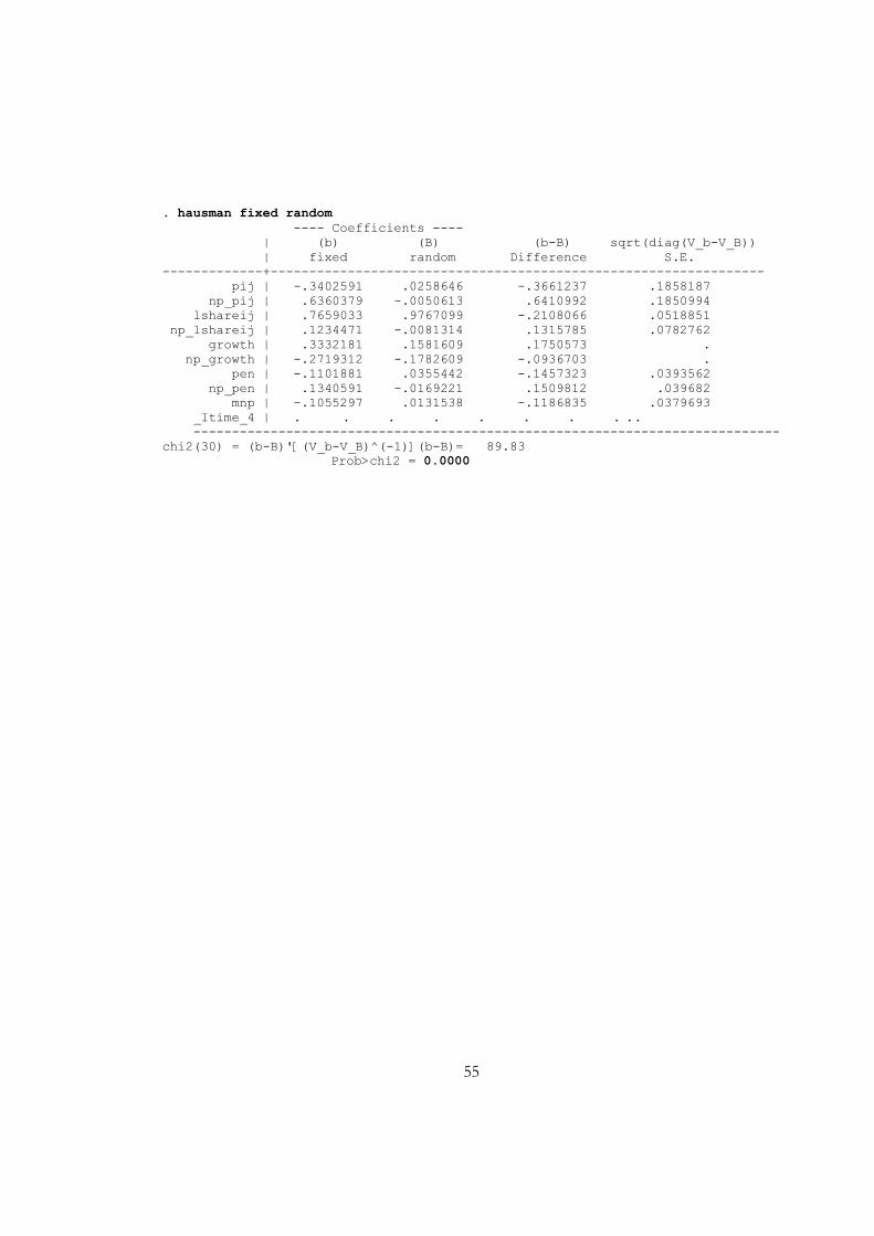
55

. hausman fixed random ---- Coefficients ---- | (b) (B) (b-B) sqrt(diag(V_b-V_B)) | fixed random Difference S.E. -------------+---------------------------------------------------------------- pij | -.3402591 .0258646 -.3661237 .1858187 np_pij | .6360379 -.0050613 .6410992 .1850994 lshareij | .7659033 .9767099 -.2108066 .0518851 np_lshareij | .1234471 -.0081314 .1315785 .0782762 growth | .3332181 .1581609 .1750573 . np_growth | -.2719312 -.1782609 -.0936703 . pen | -.1101881 .0355442 -.1457323 .0393562 np_pen | .1340591 -.0169221 .1509812 .039682 mnp | -.1055297 .0131538 -.1186835 .0379693 _Itime_4 | . . . . . . . . . . ---------------------------------------------------------------------------- chi2(30) = (b-B)'[(V_b-V_B)^(-1)](b-B)= 89.83 Prob>chi2 = 0.0000

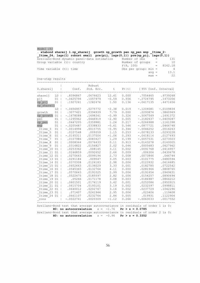
56

Model [5]

. xtabond shareij l.np_shareij growth np_growth pen np_pen mnp _Itime_2-_Itime_24, lags(1) robust small pre(pij, lags(0,1)) pre(np_pij, lags(0,1)) Arellano-Bond dynamic panel-data estimation Number of obs = 131 Group variable (i): country Number of groups = 10 F(9, 100) = 8162.18 Time variable (t): time Obs per group: min = 4 avg = 13.1 max = 22 One-step results ------------------------------------------------------------------------------ | Robust D.shareij | Coef. Std. Err. t P>|t| [95% Conf. Interval] -------------+---------------------------------------------------------------- shareij LD | .8396867 .0676623 12.41 0.000 .7054465 .9739268 pij D1 | -.0625794 .1057979 -0.59 0.556 -.2724795 .1473206 np_pij D1 | .1927261 .1282476 1.50 0.136 -.0617135 .4471656 np_shareij | LD | -.0656957 .0275772 -2.38 0.019 -.1204081 -.0109834 growth D1 | .3077421 .0394939 7.79 0.000 .2293874 .3860969 np_growth D1 | -.1678088 .1698341 -0.99 0.326 -.5047549 .1691372 pen D1 | -.1295962 .0446919 -2.90 0.005 -.2182637 -.0409287 np_pen D1 | .0447205 .0359981 1.24 0.217 -.0266988 .1161398 mnp D1 | -.0205487 .0338833 -0.61 0.546 -.0877721 .0466748 _Itime_3 D1 | -.0014994 .0015755 -0.95 0.344 -.0046252 .0016263 _Itime_5 D1 | .0107548 .009359 1.15 0.253 -.0078133 .0293228 _Itime_6 D1 | -.0145311 .0137504 -1.06 0.293 -.0418114 .0127493 _Itime_7 D1 | .0107986 .0083427 1.29 0.199 -.0057531 .0273503 _Itime_8 D1 | .0008364 .0076433 0.11 0.913 -.0143278 .0160005 _Itime_9 D1 | .0316822 .0156827 2.02 0.046 .0005683 .0627962 _Itime_10 D1 | .0253362 .008145 3.11 0.002 .0091768 .0414957 _Itime_11 D1 | .0246859 .0092652 2.66 0.009 .006304 .0430678 _Itime_12 D1 | .0270643 .0099194 2.73 0.008 .0073846 .046744 _Itime_13 D1 | .0291184 .009547 3.05 0.003 .0101775 .0480594 _Itime_14 D1 | .0370308 .0124183 2.98 0.004 .0123932 .0616685 _Itime_15 D1 | .0452663 .0136029 3.33 0.001 .0182785 .0722542 _Itime_16 D1 | .0545365 .0132764 4.11 0.000 .0281966 .0808765 _Itime_17 D1 | .0570643 .0191025 2.99 0.004 .0191654 .0949631 _Itime_18 D1 | .0522475 .0185597 2.82 0.006 .0154257 .0890694 _Itime_19 D1 | .05266 .0171178 3.08 0.003 .0186987 .0866212 _Itime_20 D1 | .0601501 .0176119 3.42 0.001 .0252086 .0950915 _Itime_21 D1 | .0615704 .0193101 3.19 0.002 .0232597 .0998811 _Itime_22 D1 | .0640012 .0202767 3.16 0.002 .0237729 .1042296 _Itime_23 D1 | .071407 .0241944 2.95 0.004 .023406 .119408 _Itime_24 D1 | .0661107 .0232764 2.84 0.005 .019931 .1122904 _cons | -.0022741 .0020309 -1.12 0.266 -.0063033 .0017552 ------------------------------------------------------------------------------ Arellano-Bond test that average autocovariance in residuals of order 1 is 0: H0: no autocorrelation z = -1.76 Pr > z = 0.0785 Arellano-Bond test that average autocovariance in residuals of order 2 is 0: H0: no autocorrelation z = -0.96 Pr > z = 0.3352