AN INVESTIGATION OF NORTH-FINDING

USING A MEMS GYROSCOPE

by

René Robért

Submitted in partial fulfillment of the

requirements for Departmental Honors in

the Department of Engineering

Texas Christian University

Fort Worth, Texas

May 2, 2014

ii

AN INVESTIGATION OF NORTH-FINDING

USING A MEMS GYROSCOPE

Project Approved:

Supervising Professor: Stephen Weis, Ph.D.

Department of Engineering

Robert Bittle, Ph.D.

Department of Engineering

Ken Richardson, Ph.D.

Department of Mathematics

iii

ABSTRACT

Navigational mapping of subsurface holes drilled for oil and gas

production is required by law. Currently, mapping a drilled hole requires the use

of expensive gyroscopes to determine azimuthal direction (e.g., North, West etc.).

However, MEMS (micro-electro-mechanical-systems) gyros are now

commercially available and are orders of magnitude less expensive than current

downhole spinning mass gyros. Unfortunately, they are not accurate enough to be

used for downhole mapping.

Determining the azimuth of a subsurface hole requires a gyro to measure a

component of the rotation of the earth. At Fort Worth’s latitude, a gyro pointed

North would measure a rotation rate of 0.0035 degrees/second; while a gyro

pointed East would measure zero degrees/second. Unfortunately, the drift of

MEMS gyro-measured rotation rate is much larger than earth’s rotation rate. Our

experimental work indicates that MEMS gyro signals can be averaged and

combined to improve the signal-to-noise ratio and subsequently reduce error.

iv

TABLE OF CONTENTS

INTRODUCTION ..............................................................................................................1

GYROSCOPES...................................................................................................................1

MEMS .................................................................................................................................2

Analog Devices AD646 ..........................................................................................2

Sensonor STIM210 .................................................................................................4

CHARACTERIZATION ....................................................................................................5

Allan Variance ........................................................................................................5

COLLECTING DATA .......................................................................................................8

Maytagging .............................................................................................................9

East-Seeking ...........................................................................................................9

Carouselling .......................................................................................................... 10

Optimum Parameters ............................................................................................ 10

Variables ............................................................................................................... 12

Table ......................................................................................................... 12

Circuit Board ............................................................................................. 12

Power Source ............................................................................................ 13

Slip Rings .................................................................................................. 13

FILTERS ........................................................................................................................... 13

Original Filter........................................................................................................ 14

Updated Filter ....................................................................................................... 16

Swanson and Schlamminger ................................................................................. 17

Next Nearest and Next Next Nearest Neighbor .................................................... 18

Sliding Average .................................................................................................... 18

CONCLUSIONS............................................................................................................... 19

v

Repeatability ......................................................................................................... 19

Ergodicity .............................................................................................................. 19

FUTURE WORK .............................................................................................................. 20

REFERENCES ................................................................................................................. 21

1

INTRODUCTION

The goal of my research project was to continue the research into determining

azimuthal north with a micro-electro-mechanical system (MEMS) gyroscope. The

application for this research is downhole mapping. Downhole mapping requires point-

by-point measurement of depth, inclination, and azimuth. Depth and inclination are

relatively easy to measure; measuring azimuth is much more difficult. The determination

of azimuthal direction done by a gyroscope is known as gyrocompassing.

Oil and gas companies in Texas are required by the Railroad Commission of

Texas to map the subsurface where they are drilling. Companies currently use a variety

of different gyroscopes for these applications such as macro-scale fiber optic, ring laser,

and quartz hemispherical resonator gyroscopes. These gyroscopes are very large and

expensive. MEMS gyroscopes are now being considered for gyrocompassing since they

are both cheaper and smaller; however, current MEMS gyroscopes’ measurements are

considered unreliable. The ultimate goal of our research is to eventually create a

procedure for taking data in about a minute that can then be filtered to determine the

earth’s rotation rate that will allow the tool to determine azimuth.

GYROSCOPES

Gyroscopes measure rotation rates and have a variety of uses. They are often

spinning bodies and can be found in toys and cellphones among others. They are even

used to balance a moving system such as a Segway. However, I will focus on their use in

measuring the rotation rate of the earth. From determining the rotation rate of the earth,

the azimuthal direction can be determined through the use of trigonometry. For example,

since we know the latitude of Fort Worth, we can determine the y-component of the

2

rotation rate at Fort Worth, rotation rate facing North.

( ) . The current gyroscopes used

for this function are very expensive, large spinning mass gyros. Our hope is that we can

substitute this kind of gyro with a MEMS gyroscope.

MEMS

MEMS or micro-electro-mechanical systems is a growing area of the electrical

sensor industry. MEMS technology has many potential applications in numerous areas.

One of the first applications of MEMS technology was in accelerometers in automobiles

to detect collisions and thus deploy airbags. MEMS devices often provide an alternative

to current technology in a chip form. MEMS gyroscopes are much less expensive and

smaller than those currently used. The problem, however, is that MEMS gyroscopes are

not as accurate as their counterparts. Through the use of filters, we hope to be able to

determine the azimuthal direction that the gyroscope is facing based on the measurement

of the rotation rate of the Earth. The two gyroscopes that were used in testing are the

Analog Devices AD646 and Sensonor STIM210.

Analog Devices AD646

The AD646 is pictured in Figure 1 and was the

less expensive of the two, costing about $135. It

measures the rotation rate of the earth through the use

of sensors inside of the chip. The chip contains inner

sensors that measure displacement due to the force

generated by the Coriolis Effect on a rotating system.

These inner sensors interact with outer sensors in order

Figure 1: Picture of the Analog

Devices AD646 MEMS

Gyroscope

3

to create a capacitive signal proportional to the angular rate based on the Coriolis Effect.

The capacitive signal is transferred to an output voltage. This output voltage can then be

converted to rotation rate in degrees/second through the use of the 0.009

V/(degrees/second) conversion rate provided by Analog Devices. Analog Devices claims

that its gyros are able to eliminate small vibrations as noise. It advertises its ability to

have vibration stability as its most important feature. The quad-sensor design contained

by the AD6464 allows for this feature. The four sensors are connected in such a way that

a new “zero” is created based on the common signal experienced by the four sensors;

therefore, the chip can eliminate both linear and angular acceleration resulting in the

rejection of shock and vibration. This is an ideal trait for the gyroscope due to the nature

of the work it will perform. The gyro will be subject to numerous vibrations during

underground measurements; therefore, to be able to filter that noise out and be left with

just the rotation rate data is important.

A common trait used to characterize the drift performance of gyroscopes is

through a parameter called bias instability. Data sheets provide a bias stability for the

given gyro that can be defined as lowest bias stability able to be achieved for the gyro. It

can be determined for a given gyro by looking at the Allen Variance of the gyro. The

lowest bias stability is the optimum parameter for taking data since it is the longest time

frame where data averaging reduces error. Analog Devices provides that the bias

instability of the AD646 is 12°/hr. This means that over the course of an hour, the gyro’s

error due to drift is 12°.

The AD646 gyroscope requires a 6 volt power supply ± 0.15 V. Since the output

of the AD646 is an analog voltage, the AD646 required a separate data acquisition

4

package called LabJack. The gyro connects to LabJack with a circuit board in order to

collect the different output signals such as ground, output voltage, and temperature. The

circuit board is also used in order to place an initial low-pass filter through the use of a

voltage divider and capacitors. LabJack connects to the computer through the use of an

USB port and reads MATLAB scripts. The gyro is mounted on an Aerotech A3200

rotation table, which is also able to be controlled by a Matlab script. Therefore, a single

script was created to control both data acquisition and the rate table.

Sensonor STIM210

The Sensonor STIM210 gyro was borrowed for a semester to perform

measurements and compare those to the AD646. The

STIM210 is a more expensive gyroscope costing $5,780;

however, it also has a much higher accuracy as seen by its

bias instability of 0.5°/hr. The Sensonor gyro is a three

axis self-contained miniature package as seen in Figure 2.

In addition to excellent performance in vibration and

shock as was true with the AD646, the STIM210 is also

compensated for drift due to temperature effects. It is

connected to the computer through the use of two USBs, one for power and the other for

data collection. Sensonor provides its own software package to handle the data

acquisition, which allowed for a simpler setup since no other hardware or software was

required to collect data or to power the gyro. The software provided a simple digital

interface that allowed the parameters of the testing to be controlled. Matlab was still used

in order to control the rotation table when running tests.

Figure 2: Picture of the

Sensonor STIM210 MEMS

Gyroscope package

5

CHARACTERIZATION

In order to minimize the amount of error in a gyroscope, it is first important to

understand the errors that are prevalent. Ideally a gyro would measure zero when it is not

experiencing any rotation; however, this is not true. Some error inducing factors include

temperature effects, null bias drift, outside forces, and incorrect characterization among

others. Bias drift is the tendency for the gyro to drift over a period of time. To minimize

the null bias of a gyro it is important to reduce all of these factors if possible. One of the

main reasons that the AD646 was chosen is that it reduces the effect that external

vibration has on a rotation measurement. The STIM210 enhances bias error reduction

even more by self-compensating for the effects of temperature. Correctly characterizing

the gyro is also an important step in order to minimize the amount of error.

Allan Variance

A common method to characterize gyroscopes is through a parameter called Allan

Variance or Allan Deviation.

( )

( )∑( ( ) ( ) )

A graph of the square root of AVAR vs τ on a log-log plot can be analyzed in order to

determine the optimum parameter to collect data. The y-axis of Allan deviation is the

bias stability of the gyro; consequently, the minimum point on the y-axis corresponds

with the ideal duration for taking data in the x-axis.

6

Analog Devices provides the Allan Deviation plot in Figure 3 in the data sheet for

the AD646. By looking at the plot, it can be determined that the minimum root Allan

Deviation or bias stability is 12°/hr corresponding to an average time between thirty and

forty seconds. Although Analog Devices characterizes each of the gyros, it is also

important to characterize the gyros that will be used for testing. To characterize the gyro

we used, data was collected for a period of time such as one hour while the gyro

remained in the same direction. This data was placed in either a script that we created in

Matlab to calculate the Allan Variance and produce a plot or a program called Alavar 5.2,

which returned similar information. The output plot of the Matlab script for the AD646

is pictured in Figure 4. As is seen by the plot, the minimum Allan Variance occurs at

34.5 seconds. The parameter that we determined through our own characterization

appears to match fairly closely to the plot from the data sheet.

Figure 3: Typical Root Allan

Deviation at 25°C vs

Averaging Time for the

AD646

7

Figure 4: Allan Variance Plot

generated with the Matlab

script for the AD646. Plot of

Allan Variance vs Averaging

Time

Sensonor provides a similar plot for root Allan Variance in their data sheet for the

STIM210 as seen in Figure 5. The minimum point of bias stability occurs at a

considerably longer duration for the STIM210, as the averaging time is about 1000

seconds for all three of the axes. Figure 6 depicts a plot of the Allan Variance for the

STIM210 that was created using Alavar 5.2. The minimum point occurs at a time

constant, τ, of 32,768 which translates to about 4.4 minutes with a bias stability of about

0.7 °/hr. However, 4.4 minutes is too great of a period to collect data, so we looked at the

point when the time constant was 2,048 and its duration was 16.4 seconds which

provided an error of 1.6°/hr. This point allowed a large tradeoff in time without

sacrificing the bias stability too greatly. These two characterization tests provided the

starting durations that were used in creating a procedure for data acquisition for each of

the gyroscopes.

8

COLLECTING DATA

After the characterizing each gyro, a procedure for collecting data for azimuthal

measurements was created. The Earth’s rotation rate can be measured using static and

dynamic methods. Static methods involve taking data while the gyro remains stationary,

while dynamic methods take data while the gyro is moving.

Figure 5: Typical Root

Allan Deviation vs

Averaging Time for

the three axes of the

STIM210

Figure 6: Allan

Deviation vs Time

Constant for the

STIM210

generated using

Alavar 5.2

9

Maytagging

For most of our testing, we used a static method called “maytagging.” This

process gets its name from the motion of a washing machine. This procedure is done by

facing the gyro in a given direction while collecting data for the desired interval. The

gyro then rotates 180° and remains there for the same interval, then returning to the

original position by rotating -180 degrees. This procedure is repeated ten times for a

single data set; therefore, measurements are taken during twenty intervals. Since Allan

Variance characterization should minimize error for 32 seconds averaging time, that was

the interval used for the AD646. Maytagging was chosen as the primary means of

measuring the Earth’s rotation rate since it allows for some cancellation of error when

calculating the rotation rate. When taking the average of the adjacent signals, some of

the bias error is removed as seen in the equation. A majority of the error is removed, but

( ) ( )

due to the nature of instability in the bias error significant error remains. In addition to

the two-point maytagging described, we also looked at four-point maytagging.

East-Seeking

Maytagging was our most successful method for measuring the rotation rate of the

Earth, but we also experimented with another static method which we called East-

Seeking. The East-Seeking algorithm builds on maytagging to find East. It involves

orienting the gyro in a random direction, and then begins maytagging at that point. After

the gyro gets a reading of its direction, it tries to correct itself based on the rotation rate

that was measured. This process is repeated until the gyro correctly measures East.

Based on the amount the gyro adjusted, we can determine which direction it was

10

originally facing. This script provided some promising results with the AD646 at first;

however, it was determined that the gyro was not stable enough in order to further

investigate the script in the current setup.

Carouselling

One dynamic method we used was “carouselling.” Carouselling involves taking

data as the gyro continually spins. The results of this test should produce a sine wave,

which can then be examined to locate specific points on the wave. The peaks would be

North and South, while the intercepts are East and West. Due to the bias noise of the

gyro, the signal was indistinguishable and was quickly deemed useless with the AD646.

Optimum Parameters

Although we determined the optimum averaging duration for each gyro, we also

experimented with various durations and column lengths. For each of the gyros, we took

data at half and double the parameter determined from Allan Variance. For the AD646,

we took data with durations of 16, 34, and 68 seconds at maytagging stops. After

comparisons between data sets, it was determined that the better results occurred at the 34

second duration. Since the STIM210 had a different characterization, we used durations

of 8, 16, and 32 seconds. The idea for taking various lengths originally started by

thinking that the Allan Variance time is actually the time for one complete cycle

compared to just one stop.

In addition to changing the duration of each stop, we also looked at the number of

columns or stops in a data set. The standard set of data originally consisted of ten

complete cycles of maytagging or twenty stops for both gyros. This was chosen

arbitrarily because a complete cycle was not too lengthy and it allowed the rotation rate

11

to be calculated as an average of ten rotation rates. We were uncertain as to whether the

number of columns was significant. We wanted to be able to somewhat definitively state

what the optimum number of columns should be as we did with the duration. To figure

out the number of columns chosen per data set for the AD646, we came up with the idea

of taking the Allan variance for all of the calculated rotation rates for a given set of data.

To do this, we took a data set of 108 columns which would give us an Allan variance

graph with six points (1,2,4,8,16,32). The Allan Variances for these runs were calculated

using Alamath 5.2. We determined that the 32 columns points had too great of an error

bar and should not be used even though they usually were the lowest value. Therefore,

we were left with the 16 columns point. This means that the optimum number of

columns per data set should be around the 16 – 20 columns per data set.

When comparing the amount of columns to the rotation rates they provided, we

saw that the rotation rate did not always improve by that much from 20 columns to 108

columns for the AD646. In fact, sometimes it got worse. Therefore, we concluded that

collecting 20 columns was better than 108 for data, especially due to the time difference

between the two. In the future, we decided to take 18 columns per data set since it is in

the middle of the range. The other common data set for the STIM210 contained 100

complete cycles. These large data sets were done to be more versatile. Although the

long data sets did not work well for the AD646, it worked really well for the STIM210.

We could look at the data set as a whole or break it into ten sets of ten rotation rates.

This also allowed for easier testing in that the gyro could be left unattended for an

extended period of time.

12

Variables

Table

Throughout the course of my research, we experimented with a number of

different experimental variables. The first major variable that was adjusted was the table

on which data was taken. The table used for the lab is an optics table. Optics tables are

designed to minimize vibrations experienced by the table. This is done by having the

legs of the table fill up with air creating an air cushion between the ground and

workspace. Optics work is very sensitive, so these tables help nullify any vibrations that

would normally be transferred through the ground. Initially, all of our testing was done

with the table “floating.” It was suggested that we try to take data when the table rested

on the actual legs with the air removed. I performed a comparison of five data sets with

each variable. Overall, when the table was resting on its legs the percent error was less

than the percent error when the table was floating, 10.9% and 16.6% respectively.

Therefore, all future testing was done while the table was resting on its legs.

Circuit Board

Another variable that was adjusted for the AD646 was the elimination of the

circuit board or breadboard. A breadboard was originally needed as a voltage divider and

in order to place a preliminary filter on the signal. The idea was that the extra wiring

required for the breadboard created extra noise, so we sought to remove it from the

system in order to compare results. To do this, we simply added the capacitors and

wiring directly into the LabJack ports. However, no noticeable result was achieved after

removing the breadboard.

13

Power Source

As mentioned previously, the AD646 required a 6 V power source. For most of

our testing we used an Agilent 6614C for this power source. It occurred to us that this

source may be noisy; therefore we looked to replacing this with 4 AA batteries. AA

batteries have a voltage of 1.5V each, so four of them should equal 6 V. However, this

was not the case. The four fully charged batteries resulted in a voltage of 6.18 V.

Connecting the four batteries to the gyro resulted in frying the AD646 chip. Although we

thought about trying the batteries as a source again after they have been drained to 6 V,

we never replaced the power source.

Slip Rings

Based on our efforts to reduce noise in the system, we also looked at using the

slip rings in the rate table. This would allow us to use shorter wires in addition to

removing the movement of the wires while the rate table is spinning. The wires were

soldered into the input at the top of the rate table. The signals then move through the rate

table through the use of slip rings. The LabJack can then be soldered to the output of the

slip rings at the back of the rate table completing the circuit once again. We tested the

viability of this option through the use of an oscilloscope. By hooking up a power source

to the input and an oscilloscope to the output, we were able to determine that the slip

rings did not seem to add measurable noise. The slip rings were used in all

subsequent testing.

FILTERS

Once the data was taken, we could then begin the filtering process in order to

determine the rotation rate measured by the gyroscope. My research with this project

14

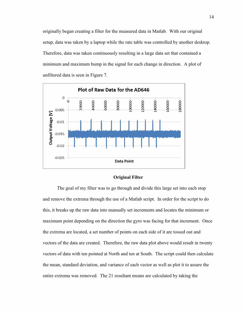
originally began creating a filter for the measured data in Matlab. With our original

setup, data was taken by a laptop while the rate table was controlled by another desktop.

Therefore, data was taken continuously resulting in a large data set that contained a

minimum and maximum bump in the signal for each change in direction. A plot of

unfiltered data is seen in Figure 7.

Original Filter

The goal of my filter was to go through and divide this large set into each stop

and remove the extrema through the use of a Matlab script. In order for the script to do

this, it breaks up the raw data into manually set increments and locates the minimum or

maximum point depending on the direction the gyro was facing for that increment. Once

the extrema are located, a set number of points on each side of it are tossed out and

vectors of the data are created. Therefore, the raw data plot above would result in twenty

vectors of data with ten pointed at North and ten at South. The script could then calculate

the mean, standard deviation, and variance of each vector as well as plot it to assure the

entire extrema was removed. The 21 resultant means are calculated by taking the

15

difference of each North mean and each of its neighbors, which are South means, and

then dividing by two. As mentioned when talking about maytagging, this is to help

reduce the offset error. This process results in twenty voltage difference values with

units of mV which can then be converted the component of the rotation rate of the earth

parallel to the Earth’s axis of rotation according to the gyro with the conversion factor of

9mV/(°/sec) to obtain 20 rotation rates. The twenty rotation rates in °/second are plotted

versus the mean of the values and the accepted value of -0.0035 degrees/second which is

the rotation rate of the earth when facing North/South for Fort Worth which is depicted in

Figure 8.

Figure 8: Plot of Rotation Rates for a run with the AD646

Rotation Rate [°/sec]

Rate Number in Data Set

16

Updated Filter

This script was eventually able to be modified once the rate table was able to be

controlled by a script in Matlab. Initially, the rate table was run on its own software

which is why two computers were needed. After the switch was made, a single computer

was able to run a script that performed all of the desired functions of spinning the rate

table, taking data, and filtering the data. The new script was also able to collect data only

while the gyroscope was stationary and create a new vector of data for each stop. The

resulting filter was able to be greatly simplified and allowed for easier collection of data.

An example of the unfiltered data for the STIM210 is seen in Figure 9 and can be

compared to the data after it has been filtered in Figure 10.

Figure 9: A plot of the X axis data (EW) for the STIM210. The multiple vectors create

the different color plots.

Rotation Rate [°/sec]

Raw Data Points

17

Swanson and Schlamminger

In addition to the nearest neighbor filter which was used, we also tried a few

others such as Swanson and Schlamminger, next nearest neighbor, next next nearest

neighbor, and a sliding average filter. The Swanson and Schlamminger is similar to the

nearest neighbor, except it places an equal weight on all vectors while ours places less

weight on the first and last vector. After a comparison between results of both filters was

made, it was determined that there was no noticeable difference in the results between the

two filters. Therefore, we decided to keep using our filter for the time being.

S & S filter = UV; with U = (data vector) and V = (

)

Figure 10: A plot of the X and Y axis data for the STIM210. The multiple vectors create the

different color plots. The circle points are for the X axis rotation rates and the star points

are for the Y axis. The red and blue lines are the accepted values for the X and Y axis

respectively. The green and black lines are the calculated values for the X and Y axis.

respectively.

Rotation Rate [°/sec]

Raw Data Points

18

Next Nearest and Next Next Nearest Neighbor

We also looked at recycling each set of data multiple times in Next Nearest

Neighbor and Next Next Nearest Neighbor. Nearest Neighbor relates three vectors of

data to each other, one North for every two South. Next Nearest Neighbor relates five

vectors to each other and Next Next Nearest neighbor relates seven. The same principle

is used for both of these; the thinking is that one can recycle data taken in the same set in

order to get more results. By reusing vectors of data, we are able to get more rotation

rates within one data set. However, these added rotation rates did not translate to better

results. Thus, the current Nearest Neighbor filter was kept once again.

Sliding Average

The sliding average filter was mainly used to look at the effect that temperature

had on the rotation rates. This script was the only one that was applied to the STIM210.

The sliding average works in such a way that it smoothes the data by making it more

linear. This data was graphically compared with temperature in another script called

moving average as seen in Figure 11. As seen, there appears to be no significant

correlation between the rotation rate data and temperature data for the STIM210.

0 0.2 0.4 0.6 0.8 1 1.2 1.4 1.6 1.8 2

x 106

0

5

10

15

20

25

0 0.2 0.4 0.6 0.8 1 1.2 1.4 1.6 1.8 2

x 106

-5

0

5

10

15

20x 10

-3

Figure 11: Plot of

Filtered

temperature and

rotation rate data

for STIM210.

Temperature is

blue and rotation

rate is green.

Temperature [°C] Rotation Rate [°/sec]

Raw Data Points

19

CONCLUSIONS

Repeatability

After numerous testing and observations have been completed, a number of

conclusions began to form for each of the gyroscopes. The most important conclusion is

that the repeatability of the gyroscopes needs to be improved. This is especially true for

the AD646. Although we were greatly improving the bias drift from the 12°/hr through

filtering to usually less than 5° for a data set, the results were not consistent. It was

determined that the signal to noise ratio for the AD646 is near 1:1. In order to get more

repeatable results, the ratio needs to greatly increase. This can be attempted by either

increasing the signal or reducing the noise. The fact that we were getting fairly accurate

results shows that we were improving upon this ratio, but it needs to be better in order to

gain consistency.

Ergodicity

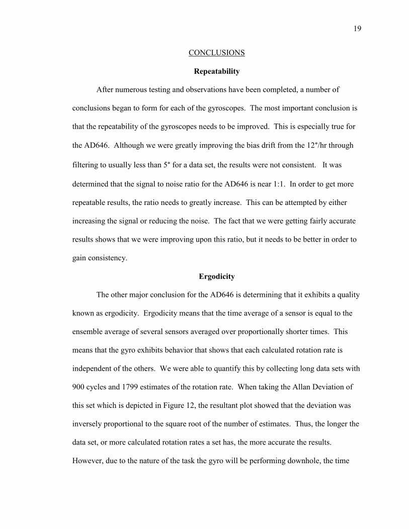
The other major conclusion for the AD646 is determining that it exhibits a quality

known as ergodicity. Ergodicity means that the time average of a sensor is equal to the

ensemble average of several sensors averaged over proportionally shorter times. This

means that the gyro exhibits behavior that shows that each calculated rotation rate is

independent of the others. We were able to quantify this by collecting long data sets with

900 cycles and 1799 estimates of the rotation rate. When taking the Allan Deviation of

this set which is depicted in Figure 12, the resultant plot showed that the deviation was

inversely proportional to the square root of the number of estimates. Thus, the longer the

data set, or more calculated rotation rates a set has, the more accurate the results.

However, due to the nature of the task the gyro will be performing downhole, the time

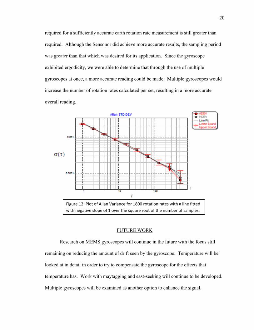
20

required for a sufficiently accurate earth rotation rate measurement is still greater than

required. Although the Sensonor did achieve more accurate results, the sampling period

was greater than that which was desired for its application. Since the gyroscope

exhibited ergodicity, we were able to determine that through the use of multiple

gyroscopes at once, a more accurate reading could be made. Multiple gyroscopes would

increase the number of rotation rates calculated per set, resulting in a more accurate

overall reading.

FUTURE WORK

Research on MEMS gyroscopes will continue in the future with the focus still

remaining on reducing the amount of drift seen by the gyroscope. Temperature will be

looked at in detail in order to try to compensate the gyroscope for the effects that

temperature has. Work with maytagging and east-seeking will continue to be developed.

Multiple gyroscopes will be examined as another option to enhance the signal.

Figure 12: Plot of Allan Variance for 1800 rotation rates with a line fitted

with negative slope of 1 over the square root of the number of samples.

21

REFERENCES

"ALAMATH." ALAMATH. Web. http://www.alamath.com/

Analog Devices. ADXRS646 Data Sheet. Web. http://www.analog.com/static/imported-

files/data_sheets/ADXRS646.pdf

Looney, Mark. "A Simple Calibration for MEMS Gyroscopes." EDN Europe July 2010:

28-31. Web. http://www.analog.com/static/imported-

files/tech_articles/GyroCalibration_EDN_EU_7_2010.pdf

Prikhodko, Igor P., Sergei A. Zotov, Alexander A. Trusov, and Andrei M. Shkel. "What

Is MEMS Gyrocompassing? Comparative Analysis of Maytagging and

Carouseling." Journal of Microelectromechanical Systems . Web.

http://mems.eng.uci.edu/files/2014/03/jmems-prikhodko-zotov-trusov-shkel-

2013.pdf

Sensonor. Sensonor STIM210 Multi-Axis Gyro Module Datasheet. Web.

http://www.sensonor.com/media/94204/ts1545.r14%20datasheet%20stim210.pdf

Sensonor. "STIM210." Sensonor AS. Web. http://www.sensonor.com/gyro-

products/gyro-modules/stim210.aspx

Sensonor. Ultra-High Performance Gyro Module STIM210 Product Brief. Web.

http://www.sensonor.com/media/72680/2013-07-30-product-brief-stim210-a4-

web.pdf