an introduction to wireless sensor networks - es.mdh.se · an introduction to wireless sensor...
TRANSCRIPT

An Introduction to Wireless Sensor Networks
2014 Swedish Communication Technologies Workshop (Swe-CTW 2014),Malardalan University, June 2-5, 2014
Carlo FischioneAssociate Professor of Sensor Networks
e-mail:[email protected]://www.ee.kth.se/∼carlofi/
KTH Royal Institute of TechnologyStockholm, Sweden
June 5, 2014Carlo Fischione (KTH) An Introduction to Wireless Sensor Networks June 5, 2014 1 / 100

Tutorial goal
After finishing the tutorial, you will know the essential networking andoptimization tools to cope with Wireless Sensor Networks (WSNs)
You will be able to design WSNs and learn recent selected researchdirections
Carlo Fischione (KTH) An Introduction to Wireless Sensor Networks June 5, 2014 2 / 100

Wireless Sensor Networks
Networking Wireless
Systems and Control
WirelessSensorNetworks
Carlo Fischione (KTH) An Introduction to Wireless Sensor Networks June 5, 2014 3 / 100

WSNs
Wireless sensor networks (WSNs) make Internet of Things possible
Computing, transmitting and receiving nodes, wirelessly networked together forcommunication, control, sensing and actuation purposes
Characteristics of WSNsI Battery-operated nodesI Short range wireless communicationI Mobility of nodesI No/limited central manager
Typical power consumption of a nodeCarlo Fischione (KTH) An Introduction to Wireless Sensor Networks June 5, 2014 4 / 100

Outline
Introduction
Medium Access Control
Routing
Cross-Layer Optimization
Distributed Optimization
Privacy Preserving Optimization
Carlo Fischione (KTH) An Introduction to Wireless Sensor Networks June 5, 2014 5 / 100

History of WSNs
DARPA DSN node, 1960
Mica2 mote, 2002
Tmote-sky, 2003
Smart Dust
Carlo Fischione (KTH) An Introduction to Wireless Sensor Networks June 5, 2014 6 / 100

Applications of WSNs
Environmental Monitoring
Transportation
Industrial Control
Healthcare
Carlo Fischione (KTH) An Introduction to Wireless Sensor Networks June 5, 2014 7 / 100

Smart Buildings
WSNs for controlling temperature, light, air and humidity, doors, alarms
Carlo Fischione (KTH) An Introduction to Wireless Sensor Networks June 5, 2014 8 / 100

Smart Buildings
By 2020, one of the most technological urban districts in the world
Thousands of Smart Buildings will be built
Carlo Fischione (KTH) An Introduction to Wireless Sensor Networks June 5, 2014 9 / 100
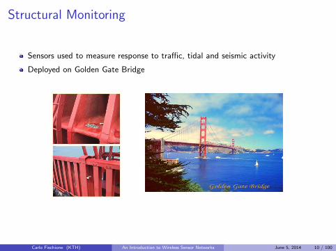
Structural Monitoring
Sensors used to measure response to traffic, tidal and seismic activity
Deployed on Golden Gate Bridge
Carlo Fischione (KTH) An Introduction to Wireless Sensor Networks June 5, 2014 10 / 100

Smart Energy Grids
source: http://deviceace.com/
Smart grids: Smart Grids: It’s All About Wireless Sensor Networks(http://stanford.wellsphere.com)
Carlo Fischione (KTH) An Introduction to Wireless Sensor Networks June 5, 2014 11 / 100

Water Pollution
The pollution level can be estimated by sensors on the water pipes
The estimates are reported centrally only when needed
Carlo Fischione (KTH) An Introduction to Wireless Sensor Networks June 5, 2014 12 / 100

WSNs in Industrial Automation
Added flexibility
I Sensor and actuator nodes can be placed more appropriatelyI Less restrictive maneuvers and control actionsI More powerful control through distributed computations
Reduced installation and maintenance costs
I Less cablingI More efficient monitoring and diagnosis
Carlo Fischione (KTH) An Introduction to Wireless Sensor Networks June 5, 2014 13 / 100

Distributed positioning
WSN allows to perform distributed camera calibration, positioning and tracking
Application: massive graphic effects in film production
Carlo Fischione (KTH) An Introduction to Wireless Sensor Networks June 5, 2014 14 / 100

Tutorial Overview
Application
Presentation
Session
Transport
Routing
MAC
Phy
Networking
Cross-Layer co-design
Optimization
Carlo Fischione (KTH) An Introduction to Wireless Sensor Networks June 5, 2014 15 / 100

Outline
Introduction
Medium Access Control
I Definition and classification of MACsI The IEEE 802.15.4 protocolI Mmwaves WSNs (the IEEE 802.15.3 protocol)
Routing
Cross-Layer Optimization
Distributed Optimization
Privacy Preserving Optimization
Carlo Fischione (KTH) An Introduction to Wireless Sensor Networks June 5, 2014 16 / 100

Next part contentApplication
Presentation
Session
Transport
Routing
MAC
Phy
When a node gets the right to transmit messages?
What is the Medium Access Control (MAC)?
What are the options to design MACs?
What is the MAC of IEEE 802.15.4?
Carlo Fischione (KTH) An Introduction to Wireless Sensor Networks June 5, 2014 17 / 100

Medium Access Control - MAC
MAC: mechanism for controlling when sending a message (packet) and whenlistening for a packet
MAC is one of the major component for energy expenditure in WSNs
I Receiving packets is about as expensive as transmittingI Idle listening for packets is also expensive
Typical power consumption of a node
Carlo Fischione (KTH) An Introduction to Wireless Sensor Networks June 5, 2014 18 / 100

Problems for MACs
1. Collisions: wasted effort when two packets collide
2. Overhearing: wasted effort in receiving a packet destined for another node
3. Idle listening: sitting idly and trying to receive when nobody is sending
4. Protocol overhead
Carlo Fischione (KTH) An Introduction to Wireless Sensor Networks June 5, 2014 19 / 100

The hidden terminal problem
Terminal, another word for node
Hidden terminal problem:
I Node A wants to send a packet to BI Node C wants to send a packet to DI Node A does not hear transmitter C sending packets that can be received by B
and D
Carlo Fischione (KTH) An Introduction to Wireless Sensor Networks June 5, 2014 20 / 100

The hidden terminal problem
A B C D
Transmit range:(depends on the channel, transmit power, )distance past which the SNR is in outage
Terminal, another word for node
Hidden terminal problem:
I Node A wants to send a packet to B
I Node C wants to send a packet to DI Node A does not hear transmitter C sending packets that can be received by B
and D
Carlo Fischione (KTH) An Introduction to Wireless Sensor Networks June 5, 2014 20 / 100

The hidden terminal problem
A B C D
Transmit range:(depends on the channel, transmit power, )distance past which the SNR is in outage
Terminal, another word for node
Hidden terminal problem:
I Node A wants to send a packet to BI Node C wants to send a packet to D
I Node A does not hear transmitter C sending packets that can be received by Band D
Carlo Fischione (KTH) An Introduction to Wireless Sensor Networks June 5, 2014 20 / 100

The hidden terminal problem
A B C D
Transmit range:(depends on the channel, transmit power, )distance past which the SNR is in outage
Terminal, another word for node
Hidden terminal problem:
I Node A wants to send a packet to BI Node C wants to send a packet to DI Node A does not hear transmitter C sending packets that can be received by B
and D
Carlo Fischione (KTH) An Introduction to Wireless Sensor Networks June 5, 2014 20 / 100

The exposed terminal problem
A B C D
Carrier sense range:(depends on the channel, transmit power,...)distance within a transmitter can be heard/sensed at a receiver
Exposed terminal problem:
I B wants to send packet to AI C wants to send packets to DI Transmitter B hears transmitter C which is not causing collisions at the
receiver A. A is not in the transmit range of CI Transmitter C hears B, but D is not in the transmit range of B
Carlo Fischione (KTH) An Introduction to Wireless Sensor Networks June 5, 2014 21 / 100

The exposed terminal problem
A B C D
Transmit range of B Transmit range of C
Carrier sense range:(depends on the channel, transmit power,...)distance within a transmitter can be heard/sensed at a receiver
Exposed terminal problem:
I B wants to send packet to AI C wants to send packets to DI Transmitter B hears transmitter C which is not causing collisions at the
receiver A. A is not in the transmit range of CI Transmitter C hears B, but D is not in the transmit range of B
Carlo Fischione (KTH) An Introduction to Wireless Sensor Networks June 5, 2014 21 / 100

The exposed terminal problem
A B C D
Transmit range of B
Carrier sense range of B
Transmit range of C
Carrier sense range of CCarrier sense range:(depends on the channel, transmit power,...)distance within a transmitter can be heard/sensed at a receiver
Exposed terminal problem:
I B wants to send packet to A
I C wants to send packets to DI Transmitter B hears transmitter C which is not causing collisions at the
receiver A. A is not in the transmit range of CI Transmitter C hears B, but D is not in the transmit range of B
Carlo Fischione (KTH) An Introduction to Wireless Sensor Networks June 5, 2014 21 / 100

The exposed terminal problem
A B C D
Transmit range of B
Carrier sense range of B
Transmit range of C
Carrier sense range of CCarrier sense range:(depends on the channel, transmit power,...)distance within a transmitter can be heard/sensed at a receiver
Exposed terminal problem:
I B wants to send packet to AI C wants to send packets to D
I Transmitter B hears transmitter C which is not causing collisions at thereceiver A. A is not in the transmit range of C
I Transmitter C hears B, but D is not in the transmit range of B
Carlo Fischione (KTH) An Introduction to Wireless Sensor Networks June 5, 2014 21 / 100

The exposed terminal problem
A B C D
Transmit range of B
Carrier sense range of B
Transmit range of C
Carrier sense range of CCarrier sense range:(depends on the channel, transmit power,...)distance within a transmitter can be heard/sensed at a receiver
Exposed terminal problem:
I B wants to send packet to AI C wants to send packets to DI Transmitter B hears transmitter C which is not causing collisions at the
receiver A. A is not in the transmit range of C
I Transmitter C hears B, but D is not in the transmit range of B
Carlo Fischione (KTH) An Introduction to Wireless Sensor Networks June 5, 2014 21 / 100

The exposed terminal problem
A B C D
Transmit range of B
Carrier sense range of B
Transmit range of C
Carrier sense range of CCarrier sense range:(depends on the channel, transmit power,...)distance within a transmitter can be heard/sensed at a receiver
Exposed terminal problem:
I B wants to send packet to AI C wants to send packets to DI Transmitter B hears transmitter C which is not causing collisions at the
receiver A. A is not in the transmit range of CI Transmitter C hears B, but D is not in the transmit range of B
Carlo Fischione (KTH) An Introduction to Wireless Sensor Networks June 5, 2014 21 / 100
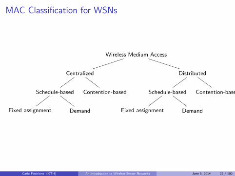
MAC Classification for WSNs
Wireless Medium Access
Centralized
Schedule-based
Fixed assignment Demand
Contention-based
Distributed
Schedule-based
Fixed assignment Demand
Contention-based
Carlo Fischione (KTH) An Introduction to Wireless Sensor Networks June 5, 2014 22 / 100

Outline
Introduction
Medium Access Control
I Definition and classification of MACsI The IEEE 802.15.4 protocolI Mmwaves WSNs (the IEEE 802.15.3 protocol) and the association problem
Routing
Cross-Layer Optimization
Distributed Optimization
Privacy Preserving Optimization
Carlo Fischione (KTH) An Introduction to Wireless Sensor Networks June 5, 2014 23 / 100

IEEE 802.15.4 protocol architecture
Now we study the MAC of the standard IEEE 802.15.4
IEEE 802.15.4 is the de-facto reference standard for low data rate and low powerWSNs
Characteristics:
I Low data rate for ad hoc self-organizing network of inexpensive fixed, portableand moving devices
I High network flexibilityI Very low power consumptionI Low cost
Carlo Fischione (KTH) An Introduction to Wireless Sensor Networks June 5, 2014 24 / 100

IEEE 802.15.4 networks
IEEE 802.15.4 network composed of
I Full-function device (FFD)I Reduced-function device (RFD)
A network includes at least one FFD
The FFD can operate in three modes:
I A personal area network (PAN)coordinator
I A coordinatorI A device
An FFD can talk to RFDs or FFDs
RFD can only talk to an FFD
Carlo Fischione (KTH) An Introduction to Wireless Sensor Networks June 5, 2014 25 / 100

IEEE 802.15.4 network topologies
PAN CoordinatorPAN Coordinator
Star topologyPeer-to-peer topology
Communication Flow
Reduced Function Device
Full Function Device
3 types of topologies
I Star topologyI Peer-to-peer topologyI Cluster-tree
Carlo Fischione (KTH) An Introduction to Wireless Sensor Networks June 5, 2014 26 / 100

Cluster-tree topology
First PAN Coordinator
PAN Coordinator
Device
Carlo Fischione (KTH) An Introduction to Wireless Sensor Networks June 5, 2014 27 / 100

IEEE 802.15.4 physical layer
Frequency bands:
I 2.4 - 2.4835GHz GHz, global, 16 channels, 250KbpsI 902.0 - 928.0MHz, America, 10 channels, 40KbpsI 868 - 868.6MHz, Europe, 1 channel, 20Kbps
Features of the PHY layer
I Activation and deactivation of the radio transceiverI Transmitting and receiving packets across the wireless channelI Energy detection (ED, from RSS)I Link quality indication (LQI)I Clear channel assessment (CCA)I Dynamic channel selection by a scanning a list of channels in search of
beacon, ED, LQI, and channel switching
Carlo Fischione (KTH) An Introduction to Wireless Sensor Networks June 5, 2014 28 / 100

IEEE 802.15.4 physical layer
1.3
2[4]*1cm PHY(MHz) 2[4]*3cmFrequency band
(MHz) Spreading parameters Data parameters3-4 6-8 3cm Chip rate
(kchip/s) Modulation 3cmBit rate(kb/s) 3cm Symbol rate
(ksymbol/s) Symbols2[4]*868/915 868-868.6 300 BPSK 20 20 Binary
902-928 600 BPSK 40 40 Binary2[4]*1cm868/915
(optional) 868-868.6 400 ASK 250 12.5 20-bit PSSS902-928 1600 ASK 250 50 5-bit PSSS
2[4]*1cm868/915(optional) 868-868.6 400 O-QPSK 100 25 16ary Orthogonal
902-928 1000 O-QPSK 250 62.5 16ary Orthogonal2450 2400-2483.5 2000 O-QPSK 250 62.5 16ary Orthogonal
Frequency bands and propagation parameters for IEEE 802.15.4 physical layer
Carlo Fischione (KTH) An Introduction to Wireless Sensor Networks June 5, 2014 29 / 100

Physical layer data unit
SFD indicates the end of the SHR and the start of the packet data
PHR: PHY headerPHY payload < 128 byte
Carlo Fischione (KTH) An Introduction to Wireless Sensor Networks June 5, 2014 30 / 100

IEEE 802.15.4 MAC
The MAC provides two services:
I Data serviceI Management service
MAC features: beacon management, channel access, GTS management, framevalidation, acknowledged frame delivery, association and disassociation
Carlo Fischione (KTH) An Introduction to Wireless Sensor Networks June 5, 2014 31 / 100

Superframes
Superframe structure:
I Format defined by the PAN coordinatorI Bounded by network beaconsI Divided into 16 equally sized slots
Beacons
I Synchronize the attached nodes, identify the PAN and describe the structureof superframes
I Sent in the first slot of each superframeI Turned off if a coordinator does not use the superframe structure
Superframe portions: active and an inactive
I Inactive portion: a node does not interact with its PAN and may enter alow-power mode
I Active portion: contention access period (CAP) and contention free period(CFP)
I Any device wishing to communicate during the CAP competes with otherdevices using a slotted CSMA/CA mechanism
I The CFP contains guaranteed time slots (GTSs)
Carlo Fischione (KTH) An Introduction to Wireless Sensor Networks June 5, 2014 32 / 100

Bibliography
P. Park, P. Di Marco, P. Soldati, C. Fischione, K. H. Johansson, “A GeneralizedMarkov Model for an Effective Analysis of Slotted IEEE 802.15.4”, in Proc. of IEEE6th International Conference on Mobile Ad-hoc and Sensor Systems 2009 (IEEEMASS 09), Macau SAR, P.R.C., October 2009. Best Paper Award.
P. Park, S. Coleri Ergen, C. Fischione, A. Sangiovanni-Vincentelli, “Duty-CycleOptimization for IEEE 802.15.4 Wireless Sensor Networks”, ACM Transactions onSensor Networks, Vol. 10, No. 1, February 2014.
C. Fischione, P. Park, S. Coleri Ergen, “Analysis and Optimization of Duty-Cycle inPreamble Based Random Access Networks”, Springer Wireless Networks, Vol. 19,Issue 7, pp. 16911707, October 2013.
P. Park, C. Fischione, K. H. Johansson, “Modeling and Stability Analysis of HybridMultiple Access in IEEE 802.15.4 Protocol”, ACM Transactions on SensorNetworks, Vol. 9, No. 2, pp. 13:1–13:55, April 2013.
P. Di Marco, P. Park, C. Fischione, K. H. Johansson, “Analytical Modeling ofMulti-hop IEEE 802.15.4 Networks”, IEEE Transactions on Vehicular Technology,Vol. 61, No. 7, pp. 3191–3208, September 2012.
Carlo Fischione (KTH) An Introduction to Wireless Sensor Networks June 5, 2014 33 / 100

Outline
Introduction
Medium Access Control
I Definition and classification of MACsI The IEEE 802.15.4 protocolI Mmwaves WSNs (the IEEE 802.15.3 protocol)
Routing
Cross-Layer Optimization
Distributed Optimization
Privacy Preserving Optimization
Carlo Fischione (KTH) An Introduction to Wireless Sensor Networks June 5, 2014 34 / 100

Mmwaves communications
Figure: Millimeter-wave spectrum, Source: Zhouyue-Khan-2011
3-300GHz spectrum → mmW bands (λ ranges from 1-100mm)
60GHz band is an unlicensed spectrum
Large amount of spectral bandwidth: 7GHz
Achievable data rates > 2Gbps
Carlo Fischione (KTH) An Introduction to Wireless Sensor Networks June 5, 2014 35 / 100

Mmwaves communications
Figure: Variation in Received Power with 32mW transmit power at 5.1GHz (left)and 60GHz (right), Source: Williamson-Athanasiadou-Nix-1997
Does not penetrate most solid materials → extra spatial isolation
Coverage is defined by the perimeter of the room
Frequency reuse is viable
Implicit security
Carlo Fischione (KTH) An Introduction to Wireless Sensor Networks June 5, 2014 36 / 100

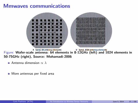
Mmwaves communications
Figure: Wafer-scale antenna: 64 elements in 8-12GHz (left) and 1024 elements in50-75GHz (right), Source: Mohamadi-2006
Antenna dimension ∝ λ
More antennas per fixed area
MIMO → higher beamforming gain / higher directivity
MIMO → SDMA → (point to multipoint communication)
Carlo Fischione (KTH) An Introduction to Wireless Sensor Networks June 5, 2014 37 / 100

Mmwaves communications
Figure: Beam comparison
Narrow beams
Interference immunity
Deployment of multiple independent links in close proximity
Point-to-point mesh networks
Carlo Fischione (KTH) An Introduction to Wireless Sensor Networks June 5, 2014 38 / 100

Mmwaves communications
Figure: Beam comparison
Narrow beams
Interference immunity
Deployment of multiple independent links in close proximity
Point-to-point mesh networks
Carlo Fischione (KTH) An Introduction to Wireless Sensor Networks June 5, 2014 38 / 100

Mmwaves communications
Figure: Beam comparison
Narrow beams
Interference immunity
Deployment of multiple independent links in close proximity
Point-to-point mesh networks
Carlo Fischione (KTH) An Introduction to Wireless Sensor Networks June 5, 2014 38 / 100

Mmwaves communications
Figure: Beam comparison
Narrow beams
Interference immunity
Deployment of multiple independent links in close proximity
Point-to-point mesh networks
Carlo Fischione (KTH) An Introduction to Wireless Sensor Networks June 5, 2014 38 / 100

Mmwaves 60 GHz Wireless Standards
IEEE 802.11ad
WiGig
IEEE 802.15.3c
WirelessHD
ECMA-387
Carlo Fischione (KTH) An Introduction to Wireless Sensor Networks June 5, 2014 39 / 100

Applications
Carlo Fischione (KTH) An Introduction to Wireless Sensor Networks June 5, 2014 40 / 100

Association Control and Relaying in60 GHz Wireless Access Networks
Carlo Fischione (KTH) An Introduction to Wireless Sensor Networks June 5, 2014 41 / 100

Association Control and Relaying in60 GHz Wireless Access Networks
Carlo Fischione (KTH) An Introduction to Wireless Sensor Networks June 5, 2014 42 / 100

Association Control and Relaying in60 GHz Wireless Access Networks
Goal: Maximizing the sum of clients’ throughput guaranteeingfair connection distribution for access points (AP)
Solution: Distributed algorithm for client-relay and client-access-point associationbased on auction algorithm
Results: Theoretical and numerical analysis
Carlo Fischione (KTH) An Introduction to Wireless Sensor Networks June 5, 2014 43 / 100

System Model
Client i ∈M = {1, . . . ,M}, relay j ∈ N = {1, . . . , N} and APk ∈ K = {1, . . . ,K}
Achievable rate at distance d is
R(d) =W log2
(1 +
PTGRGTλ2dη0
16π2(N0 + I)Wdη
)
Carlo Fischione (KTH) An Introduction to Wireless Sensor Networks June 5, 2014 44 / 100
W System bandwidth
λ Wavelength
d, d0 Distance, far field reference distance
η Path loss exponent (η ∈ [2, 6])
PT Transmission power of AP i to client j
GT ,GR Power gain of transmitter and receiver
N0 Power spectral density of the noise
I Broadband interferencei = 1 i = 3
i = 2
j = 1
23 (Q3)
45
6
7 8
9
10
R33R13

System Model
Throughput benefit from client i
a(i,k) = R(dik), a(i,j,k) = min{R(dij), R(djk)}
Total throughput
u =∑
(i,k)∈A
a(i,k)x(i,k) +∑
(i,j,k)∈A
a(i,j,k)x(i,j,k) ,
Binary decision variables x(i,k) = 1 if client i is associated to AP k and x(i,k) = 0otherwise
x(i,j,k) = 1 if client i is associated to relay j and then to AP k, or x(i,j,k) = 0otherwise
Carlo Fischione (KTH) An Introduction to Wireless Sensor Networks June 5, 2014 45 / 100

Resource Association Problem Formulation
maximizex(i,k), x(i,j,k)
u
s.t.∑
(i,k)∈A
x(i,k) +∑
(i,j,k)∈A
x(i,j,k) = 1, ∀i ∈M ,
∑(i,j,k)∈A
x(i,j,k) ≤ 1, ∀j ∈ N ,
x(i,j,k), x(i,k) = {0, 1}, ∀(i, j), (i, j, k) ∈ A ,
Variable: x(i,k), x(i,j,k)
Constraints: a) Client i needs to be assigned to one AP, b) Relay j can only beassigned to one client-AP pair, c) The decision variables are binary
Carlo Fischione (KTH) An Introduction to Wireless Sensor Networks June 5, 2014 46 / 100
i = 1 i = 3
i = 2
j = 1
23 (Q3)
45
6
7 8
9
10
R33R13

Bibliography
G. Athanasiou, C. Weeraddana, C. Fischione, L. Tassiulas, “Optimizing ClientAssociation in 60GHz Wireless Access Networks”, IEEE/ACM Transactions onNetworking, Accepted for Publication, 2014, to Appear.
G. Athanasiou, C. Weeraddana, C. Fischione, “Auction-based Resource Allocationin Millimeter-Wave Wireless Access Networks”, IEEE Communications Letters, Vol.17, No. 11, pp. 2108 2111, November 2013.
Carlo Fischione (KTH) An Introduction to Wireless Sensor Networks June 5, 2014 47 / 100

Outline
Introduction
Medium Access Control
Routing
I Classification of routing protocols for WSNsI The shortest path routingI Routing algorithms for standardized protocol stack
Cross-Layer Optimization
Distributed Optimization
Privacy Preserving Optimization
Carlo Fischione (KTH) An Introduction to Wireless Sensor Networks June 5, 2014 48 / 100

Previous partApplication
Presentation
Session
Transport
Routing
MAC
Phy
When a node gets the right to transmit?
What is the mechanism to get such a right?
How nodes are associated to access points?
Carlo Fischione (KTH) An Introduction to Wireless Sensor Networks June 5, 2014 49 / 100

Next SectionApplication
Presentation
Session
Transport
Routing
MAC
Phy
On which path messages should be routed?
What are the basic routing options?
How to compute the shortest path?
Which routing is used in standard protocols?
Carlo Fischione (KTH) An Introduction to Wireless Sensor Networks June 5, 2014 50 / 100

Routing protocols
Derive a mechanism that allows a packet sent from an arbitrary node to arrive atsome destination node
I Routing information: data structures (e.g., tables) on how a given destinationnode can be reached by a source node
I Forwarding: Consult these data structures to forward a given packet to itsnext hop node
Challenges
I Nodes may move, neighborhood relations change
Carlo Fischione (KTH) An Introduction to Wireless Sensor Networks June 5, 2014 51 / 100

Routing protocols classification
When the routing protocol operates?
1. Proactive: protocol always tries to keep its routing tables up-to-date and activebefore tables are actually needed
Example: Destination Sequence Distance Vector (DSDV), usesBellman-Ford algorithm (see below)
2. On demand: route is only determined when needed by a nodeExample: Ad hoc On Demand Distance Vector (AODV), nodes remember
where packets came from and populate routing tables accordingly
3. Hybrid: combine the previous two
Carlo Fischione (KTH) An Introduction to Wireless Sensor Networks June 5, 2014 52 / 100

But how paths are built and chosen?
We have seen a general classification of routing
In practice,
I How the routing structures (e.g., the tables) are built?I How the decision to select next hop is taken?
Carlo Fischione (KTH) An Introduction to Wireless Sensor Networks June 5, 2014 53 / 100

Many options for routing1. Path with minimum delay
2. Path with minimum packet error rate
3. Path with maximum total availablebattery capacity
I Path metric: Sum of batterylevels
I Example: A-C-F-H
4. Path with minimum battery cost
I Path metric: Sum of reciprocalbattery levels
I Example: A-D-H
5. Path with conditional max-min batterycapacity
I Only take battery level intoaccount when below a given level
6. Path with minimum variance in batterypower levels
7. Path with minimum total transmissionbattery powerCarlo Fischione (KTH) An Introduction to Wireless Sensor Networks June 5, 2014 54 / 100

Outline
Introduction
Medium Access Control
Routing
I Classification of routing protocols for WSNsI The shortest path routingI Routing algorithms for standardized protocol stack
Cross-Layer Optimization
Distributed Optimization
Privacy Preserving Optimization
Carlo Fischione (KTH) An Introduction to Wireless Sensor Networks June 5, 2014 55 / 100

The shortest path routing
i
jts
source destination
The shortest path routing problem is a general optimization problem that modelsALL the cases above for routing
In the following, we study the basic version, when in the network there is one sourceand one destination
Multiple sources multiple destinations scenarios are a simple extension
Carlo Fischione (KTH) An Introduction to Wireless Sensor Networks June 5, 2014 56 / 100

Definitions
i
jts
source destination
N Number of nodesN Set of nodesA = {(i, j)} Set of arcsG = (N ,A) Networkaij Routing cost on the link ij
Examples: 1) MAC delay i→ j 2) packet error rate i→ j
What is the shortest (minimum cost) path from source s to destination t ?
Carlo Fischione (KTH) An Introduction to Wireless Sensor Networks June 5, 2014 57 / 100

The Shortest Path optimization Problem
minx
∑(i,j)∈A
aijxij
s.t.∑
j:(i,j)∈A
xij −∑
j:(j,i)∈A
xji = si
1 if i = s
−1 if i = t
0 otherwise
xij ≥ 0 ∀(i, j) ∈ A
x = [x12, x13, ..., xin , xin+1 , ...]
xij is a binary variable. It can be also real, but remarkably if the optimizationproblem is feasible, the unique optimal solution is binary
The optimal solution gives the shorstest path source-destination
Carlo Fischione (KTH) An Introduction to Wireless Sensor Networks June 5, 2014 58 / 100

The Shortest Path Optimization Problem
minx
∑(i,j)∈A
aijxij
s.t.∑
j:(i,j)∈A
xij −∑
j:(j,i)∈A
xji = si
1 if i = s
−1 if i = t
0 otherwise
xij ≥ 0 ∀(i, j) ∈ A
This problem is much more general and can be applied to
1. Routing over WSNs, used in ROLL RPL, WirelessHART...2. Project management3. The paragraphing problem4. Dynamic programming5. ...
Carlo Fischione (KTH) An Introduction to Wireless Sensor Networks June 5, 2014 59 / 100
How to solve the Shortest Path Problem
Since it is an optimization problem, one could use standard techniques ofoptimization theory, such as Lagrangian methods
However, the solution can be achieved by combinatorial algorithms that don’t useoptimization theory at all
We consider now such a combinatorial solution algorithm, the Generic shortest pathalgorithm
The Generic shortest path algorithm is the foundation of other more advancedalgorithms widely used for routing (e.g., in ROLL RPL) such as
1. Bellman-Ford method (see exercises)2. Dijkstra method (see exercises)
Carlo Fischione (KTH) An Introduction to Wireless Sensor Networks June 5, 2014 60 / 100

Complementary slackness conditionsfor the Shortest Path Problem
A label associated to a node
dj =
{a scalar
∞
PropositionLet d1, d2, ..., dN be scalars such that
dj ≤ di + aij , ∀(i, j) ∈ A
Let P be a path starting at a node i1 and ending at a node ik. If
dj = di + aij , ∀(i, j) of P
then P is a shortest path from i1 to ik.
Carlo Fischione (KTH) An Introduction to Wireless Sensor Networks June 5, 2014 61 / 100

Generic Shortest Path Algorithm: the idea in-nuce
Complementary Slackness conditions (CS) is the foundation of the generic shortestpath algorithm
Some initial vector of labels is assigned to nodes (d1, d2, ..., dN )
The arcs (i, j) that violate the CS condition dj > di + aij are selected and theirlabels redefined so that
dj := di + aij
This redefinition is continued until the CS condition dj ≤ di + aij is satisfied for allarcs (i, j)
Carlo Fischione (KTH) An Introduction to Wireless Sensor Networks June 5, 2014 62 / 100

Iterations of the Generic Shortest Path Algorithm
Let initially be V = {1} d1 = 0, di =∞, ∀i 6= 1
Iteration of the Generic Shortest Path Algorithm
Remove a node i from the candidate list V . For each outgoing arc (i, j) ∈ A, ifdj > di + aij , set
dj := di + aij
and add j to V if it does not already belong to V
The removal rule gives
Bellman-Ford method
Dijkstra method
Carlo Fischione (KTH) An Introduction to Wireless Sensor Networks June 5, 2014 63 / 100

An example
2
1 4
3
Origin
3
1
1 1
3
2
Iteration Candidate List V Node Labels Node out of V
1 {1} (0,∞,∞,∞) 12 {2, 3} (0,3,1,∞) 23 {3, 4} (0,3,1,5) 34 {4, 2} (0,2,1,4) 45 {2} (0,2,1,4) 2
∅ (0,2,1,4)
Generic shortest path algorithm [Bertsekas, 1998]
Carlo Fischione (KTH) An Introduction to Wireless Sensor Networks June 5, 2014 64 / 100
Convergence of the algorithm (a)
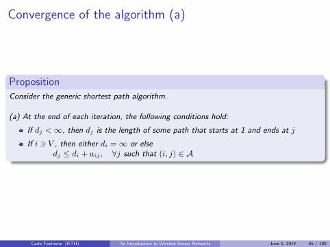
PropositionConsider the generic shortest path algorithm.
(a) At the end of each iteration, the following conditions hold:
If dj <∞, then dj is the length of some path that starts at 1 and ends at j
If i 3 V , then either di =∞ or elsedj ≤ di + aij , ∀j such that (i, j) ∈ A
Carlo Fischione (KTH) An Introduction to Wireless Sensor Networks June 5, 2014 65 / 100

Convergence of the algorithm (b)
Proposition
(b) If the algorithm terminates, then upon termination, for all j with dj <∞, dj is theshortest distance from 1 to j and
dj=
{min(i,j)∈A(di + aij) if j 6= 1
0 if j = 1
Carlo Fischione (KTH) An Introduction to Wireless Sensor Networks June 5, 2014 66 / 100

Convergence of the algorithm (c) (d)
Proposition
(c) If the algorithm does not terminate, then there exists some node j and a sequence ofpaths that start at 1, ends at j, and have a length diverging to −∞
(d) The algorithm terminates if and only if there is no path that starts at 1 and containsa cycle with negative length.
Carlo Fischione (KTH) An Introduction to Wireless Sensor Networks June 5, 2014 67 / 100

The convergence properties ofthe Generic Shortest Path Algorithm
The convergence properties above are based on sound theoretical analysis
They are the foundation over which routing protocols, such as the standardizedROLL RPL, are built
Let’s have a quick look at ROLL RPL and other standardized routing protocols
Carlo Fischione (KTH) An Introduction to Wireless Sensor Networks June 5, 2014 68 / 100

Outline
Introduction
Medium Access Control
Routing
I Classification of routing protocols for WSNsI The shortest path routingI Routing algorithms for standardized protocol stack
Cross-Layer Optimization
Distributed Optimization
Privacy Preserving Optimization
Carlo Fischione (KTH) An Introduction to Wireless Sensor Networks June 5, 2014 69 / 100

ROLL: Routing over Low Power Lossy Networks
ROLL is a Working Group of the Internet Engineering Task Forcewww.ietf.org/dyn/wg/charter/roll-charter.html
ROLL RPL, IPv6 Routing Protocol for Low Power and Lossy Networks
RPL is intended for
I Industrial and home automationI HealthcareI Smart grids
Carlo Fischione (KTH) An Introduction to Wireless Sensor Networks June 5, 2014 70 / 100

ROLL RPL assumptions
Networks with many embedded nodes with limited power, memory, and processing
Networks interconnected by a variety of protocols, such as IEEE 802.15.4,Bluetooth, Low Power WiFi, wired or other low power Powerline communications
End-to-end Internet Protocol-based solution to avoid the problem ofnon-interoperable networks interconnected by protocol translation gateways andproxies
Traffic patterns
I Multipoint to Point (MP2P)I Point to Multipoint (P2MP)I Point-to-Point (P-2-P)
Carlo Fischione (KTH) An Introduction to Wireless Sensor Networks June 5, 2014 71 / 100
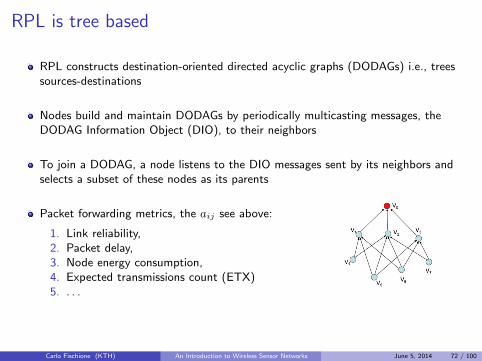
RPL is tree based
RPL constructs destination-oriented directed acyclic graphs (DODAGs) i.e., treessources-destinations
Nodes build and maintain DODAGs by periodically multicasting messages, theDODAG Information Object (DIO), to their neighbors
To join a DODAG, a node listens to the DIO messages sent by its neighbors andselects a subset of these nodes as its parents
Packet forwarding metrics, the aij see above:
1. Link reliability,2. Packet delay,3. Node energy consumption,4. Expected transmissions count (ETX)5. . . .
Carlo Fischione (KTH) An Introduction to Wireless Sensor Networks June 5, 2014 72 / 100

RPL DIO messages
DODAG minimizes the cost to go to the root (destination node) based on theObjective Function
DIO messages are broadcast to build the tree; DIO includes
I A nodes rank (its level) djI Packet forwarding metric aij
A node selects a parent based on the received DIO message and calculates its rank
Destination Advertisement Option (DAO) messages are sent periodically to notifyparent about routes to children nodes
Carlo Fischione (KTH) An Introduction to Wireless Sensor Networks June 5, 2014 73 / 100

Example
0
1 1
1
1 1 1
1
1 1 11
1
Carlo Fischione (KTH) An Introduction to Wireless Sensor Networks June 5, 2014 74 / 100

Example
0
1 1
1
1 1 1
1
1 1 11
1
DIO DIO
DIO
Carlo Fischione (KTH) An Introduction to Wireless Sensor Networks June 5, 2014 74 / 100

Example
0
1 1
1
1 1 1
1
1 1 11
11 1
1
Carlo Fischione (KTH) An Introduction to Wireless Sensor Networks June 5, 2014 74 / 100

Example
0
1 1
1
1 1 1
1
1 1 11
11 1
1DIO
DIO
DIO DIO
Carlo Fischione (KTH) An Introduction to Wireless Sensor Networks June 5, 2014 74 / 100

Example
0
1 1
1
1 1 1
1
1 1 11
11 1
1
2 2
Carlo Fischione (KTH) An Introduction to Wireless Sensor Networks June 5, 2014 74 / 100

Example
0
1 1
1
1 1 1
1
1 1 11
11 1
1
2 2
DIO DIO
DIO DIO
Carlo Fischione (KTH) An Introduction to Wireless Sensor Networks June 5, 2014 74 / 100

Example
0
1 1
1
1 1 1
1
1 1 11
11 1
1
2 2 3
Carlo Fischione (KTH) An Introduction to Wireless Sensor Networks June 5, 2014 74 / 100

Example
0
1 1
1
1 1 1
1
1 1 11
11 1
1
2 2 3
DIO
DIO
DIO DIO
DIO
Carlo Fischione (KTH) An Introduction to Wireless Sensor Networks June 5, 2014 74 / 100

Example
0
1 1
1
1 1 1
1
1 1 11
11 1
1
2 2
2
2
Carlo Fischione (KTH) An Introduction to Wireless Sensor Networks June 5, 2014 74 / 100

Example
0
1 1
1
1 1 1
1
1 1 11
11 1
1
2 2
2
2
3 3 33
2
Carlo Fischione (KTH) An Introduction to Wireless Sensor Networks June 5, 2014 74 / 100

Other standardized protocol stacks
ZigBee, www.zigbee.org
ISA SP-100, www.isa.org
WirelessHART, www.hartcomm.org
Carlo Fischione (KTH) An Introduction to Wireless Sensor Networks June 5, 2014 75 / 100

Bibliography
P. Di Marco, C. Fischione, K. H. Johansson, F. Santucci “Modeling Cross-LayerInteractions of IEEE 802.15.4 over Fading Channel”, IEEE Transactions on WirelessCommunications, to Appear, 2014.
P. Di Marco, G. Athanasiou, V. Mekikis, C. Fischione, “MAC and RoutingInteractions in Low Power and Lossy Networks”, Submitted to Computer Networks.
P. Di Marco, G. Athanasiou, C. Fischione, “Harmonizing MAC and Routing in LowPower and Lossy Networks”, in Proc. of IEEE Global TelecommunicationsConference 2013, (IEEE Globecom 13), Atlanta, GA, USA, December 2013.
P. Di Marco, G. Athanasiou, C. Fischione, “Harmonizing MAC and Routing in LowPower and Lossy Networks”, in Proc. of IEEE Global TelecommunicationsConference 2013, (IEEE Globecom 13), Atlanta, GA, USA, December 2013.
C. Fischione, S. C. Ergen, and C. Borean, “Method for Setting the OptimalOperation of a Routing Node of an Asynchronous Wireless CommunicationNetwork, Network Node and Communication Network Implementing the Method”,International Patent.
Carlo Fischione (KTH) An Introduction to Wireless Sensor Networks June 5, 2014 76 / 100

Outline
Introduction
Medium Access Control
Routing
Cross-Layer Optimization
Distributed Optimization
Privacy Preserving Optimization
Carlo Fischione (KTH) An Introduction to Wireless Sensor Networks June 5, 2014 77 / 100

Cross-Layer Optimization
Plant/Process
x(t)x(kh) sampled state
WSNIEEE 802.15.4
Wireless HART
Controlleru(t)
u(kh) sampled
actuationline
y(t)y(kh) sampled communication
line
How to co-design applications (e.g. control) and protocols?
Carlo Fischione (KTH) An Introduction to Wireless Sensor Networks June 5, 2014 78 / 100

Cross-Layer design
Energy consumption E (x)
minxE (x)
s.t. Pr (succ) ≥ 1− pPr (delay ≤ τmax) ≥ δ
x collects the protocol and control parameters
Carlo Fischione (KTH) An Introduction to Wireless Sensor Networks June 5, 2014 79 / 100

Cross-Layer design
Protocol parameters:radio powers, MACretransmissions,routing path, controldecisions...
Model methematicallythe protocol behaviour
Select the metrics(energy, delay, reliability)
Optimize (statically oron-line) the protocolparameters
Application requirements A highly efficient WSN
The role of mathematical modeling and optimization is central
Carlo Fischione (KTH) An Introduction to Wireless Sensor Networks June 5, 2014 80 / 100

Bibliography
U. Tiberi, C. Fischione, M. Di Benedetto, K. H. Johansson, “Energy-efficientSampling of Networked Control Systems over IEEE 802.15.4 Wireless Networks”,Automatica, Vol. 49, No. 3, pp. 712724, March 2013.
C. Fischione, P. Park, P. Di Marco, K. H. Johansson, “Design Principles of WirelessSensor Networks Protocols for Control Applications”, S. Mazumder Ed., Springer,Chapter 11, pp. 271299, April 2011.
P. Park, C. Fischione, A. Bonivento, K. H. Johansson, A. Sangiovanni-Vincentelli,“Breath: a Self-Adapting Protocol for Industrial Control Applications UsingWireless Sensor Networks”, IEEE Transactions on Mobile Computing, Vol. 6, No.6, pp. 821838, June 2011.
A. Bonivento, C. Fischione, L. Necchi, F. Pianegiani, A. Sangiovanni-Vincentelli,“System Level Design for Clustered Wireless Sensor Networks”, IEEE Transactionson Industrial Informatics, Vol. 3, No. 3, pp. 202214, August 2007. Best Paper ofthe IEEE Transactions on Industrial Informatics 2007.
Carlo Fischione (KTH) An Introduction to Wireless Sensor Networks June 5, 2014 81 / 100

Outline
Introduction
Medium Access Control
Routing
Cross-Layer Optimization
Distributed Optimization
Privacy Preserving Optimization
Carlo Fischione (KTH) An Introduction to Wireless Sensor Networks June 5, 2014 82 / 100

Distributed optimization
min f0(x)s.t. x ∈ X
At some “centralized” location, collect all primal variables of the network
Use primal information to calculate dual (Lagrangian) variables
Distribute dual variables over the network
Use dual variables when updating primal variables
Carlo Fischione (KTH) An Introduction to Wireless Sensor Networks June 5, 2014 83 / 100

Distributed optimization
min f0(x)s.t. x ∈ X
xi
xj
At some “centralized” location, collect all primal variables of the network
Use primal information to calculate dual (Lagrangian) variables
Distribute dual variables over the network
Use dual variables when updating primal variables
Carlo Fischione (KTH) An Introduction to Wireless Sensor Networks June 5, 2014 83 / 100

Distributed optimization
min f0(x)s.t. x ∈ X
λ
λ
At some “centralized” location, collect all primal variables of the network
Use primal information to calculate dual (Lagrangian) variables
Distribute dual variables over the network
Use dual variables when updating primal variables
Carlo Fischione (KTH) An Introduction to Wireless Sensor Networks June 5, 2014 83 / 100

Distributed optimization
min f0(x)s.t. x ∈ X
At some “centralized” location, collect all primal variables of the network
Use primal information to calculate dual (Lagrangian) variables
Distribute dual variables over the network
Use dual variables when updating primal variables
Carlo Fischione (KTH) An Introduction to Wireless Sensor Networks June 5, 2014 83 / 100

Fixed point solutions are powerfulInterference function optimization
s1
r1s2
r2
s3 r3
g11g21
Intended communicationInterference
Minimize the transmit powers whilemaintaining acceptable SINR
giipi∑i6=j
gijpj + ηi≥ γ
min ps.t. pi ≥ Ii(p) ∀i
If each interference function Ii is standard[Yates (95)], i.e.,
Monotonicity: If p ≥ p′, then I(p) ≥ I(p′)Scalability: For all α > 1, αI(p) > I(αp)
then pk+1 = I(pk) will converge to the optimal solution
Carlo Fischione (KTH) An Introduction to Wireless Sensor Networks June 5, 2014 84 / 100

Fast-Lipschitz optimization
Which problemsmax f0(x)s.t. xi ≤ fi(x) ∀i
can be solved by iteratingxk+1i = fi(x
k)?
Problem need not be convex
No need to compute, and communicate, dual variables
No central master, all nodes are peers
Nodes only need to evaluate their own constraint function
Carlo Fischione (KTH) An Introduction to Wireless Sensor Networks June 5, 2014 85 / 100

Definition of Fast-Lipschitz form
DefinitionA problem is on Fast-Lipschitz form if it can be written
max f0(x)s.t. xi ≤ fi(x) ∀i ∈ I
xi = fi(x) ∀i ∈ Ex ∈ D ⊆ <n
x = [x1, . . . , xn]T , f = [f1, . . . , fn]
T
f0 possibly vector valued, f0 : D ⊂ <n → <m, m ≥ 1
I and E are complementary subsets of {1, . . . , n}D is a box constraint,
D = {x ∈ <n |a ≤ x ≤ b}
Carlo Fischione (KTH) An Introduction to Wireless Sensor Networks June 5, 2014 86 / 100

Definition of Fast-Lipschitz problem
max f0(x)s.t. xi ≤ fi(x) ∀i ∈ I
xi = fi(x) ∀i ∈ Ex ∈ D ⊆ <n
f(x) = [f1(x), . . . , fn(x)]T
DefinitionA problem is Fast-Lipschitz when it can be written on Fast-Lipschitz form and, iffeasible, admits a unique Pareto optimal solution x?, uniquely determined by the systemof equations
x? = f(x?).
Fast-Lipschitz optimization is an alternative to dual-based methods that
I is easily distributed, low coordinationI has a low cost for communicationI is computationally cheap
Carlo Fischione (KTH) An Introduction to Wireless Sensor Networks June 5, 2014 87 / 100

Main result
max f0(x)s.t. xi ≤ fi(x) ∀i ∈ I
xi = fi(x) ∀i ∈ Ex ∈ D ⊆ <n
TheoremWhen a problem on Fast-Lipschitz form is feasible, with f0 and f fulfilling the Qualifyingconditions, the problem is Fast-Lipschitz, i.e., the unique Pareto optimal solution is givenby
x? = f(x?).
The optimal solution can then be found in a distributed manner, by iterating theconstraint functions:
xk+1 =[f(xk)
]D, or xk+1
i =[fi(x
k)]D
Qualifying conditions are sets of assumptions on f0, f and D which ensure that theproblem is Fast-Lipschitz (sufficient but not necessary)
Carlo Fischione (KTH) An Introduction to Wireless Sensor Networks June 5, 2014 88 / 100

Applications of Fast-Lipschitz problem
Fast-Lipschitz optimization is an alternative to dual-based methods for resourceallocation over wireless sensor networks and wireless networks in general
Radio power control: Interference function, Type I, Type II, functions
Distributed detection
Application to distributed estimation
Carlo Fischione (KTH) An Introduction to Wireless Sensor Networks June 5, 2014 89 / 100

Bibliography
C. Fischione, “Fast-Lipschitz Optimization with Wireless Sensor NetworksApplications”, IEEE Transactions on Automatic Control, Vol. 56, No. 10, pp. 23192331, October 2011.
M. Jakobsson, C. Fischione, C. Weeraddana, “Extensions of Fast-LipschitzOptimization”, Submitted to IEEE Transactions on Automatic Control,http://arxiv.org/abs/1309.0462.
M. Jakobsson, C. Fischione, “Optimality of Radio Power Control Algorithms viaFast-Lipschitz Optimization”, Submitted to IEEE Transactions on InformationTheory, http://arxiv-web3.library.cornell.edu/abs/1404.4947.
A. Speranzon, C. Fischione, K. H. Johansson, A. Sangiovanni-Vincentelli, “ADistributed Minimum Variance Estimator for Sensor Networks”, IEEE Journal onSelected Areas in Communications, special issue on Control and Communications,Vol. 26, No. 4, pp. 609621, May 2008.
P. C. Weeraddana, M. Codreanu, M. Latva-aho, A. Ephremides and C. Fischione,“A Review of Weighted Sum-Rate Maximization in Wireless Networks”, NOWFoundations and Trends in Networking, Vol. 6, No 1-2, pp. 1–163, 2012.
Carlo Fischione (KTH) An Introduction to Wireless Sensor Networks June 5, 2014 90 / 100

Outline
Introduction
Medium Access Control
Routing
Cross-Layer Optimization
Distributed Optimization
Privacy Preserving Optimization
Carlo Fischione (KTH) An Introduction to Wireless Sensor Networks June 5, 2014 91 / 100

Motivation – Why Privacy/Security ?
social networks
healthcare data
e-commerce
banks, and government services
Carlo Fischione (KTH) An Introduction to Wireless Sensor Networks June 5, 2014 92 / 100

Motivation – Why Privacy/Security ?
social networks
healthcare data
e-commerce
banks, and government services
Carlo Fischione (KTH) An Introduction to Wireless Sensor Networks June 5, 2014 92 / 100

Motivation – Why Privacy/Security ?
social networks
healthcare data
e-commerce
banks, and government services
Carlo Fischione (KTH) An Introduction to Wireless Sensor Networks June 5, 2014 92 / 100

Motivation – Why Privacy/Security ?
social networks
healthcare data
e-commerce
banks, and government services
Carlo Fischione (KTH) An Introduction to Wireless Sensor Networks June 5, 2014 92 / 100

Motivation – Why Privacy/Security ?
social networks
healthcare data
e-commerce
banks, and government services
Carlo Fischione (KTH) An Introduction to Wireless Sensor Networks June 5, 2014 92 / 100

Real World
example 1
- hospitals coordinate ⇒ inference for better diagnosis- larger data sets ⇒ higher the accuracy of the inference- challenge: neither of the data set should be revealed
Carlo Fischione (KTH) An Introduction to Wireless Sensor Networks June 5, 2014 93 / 100
anchor
data set 1 data set 2
data set 3hospital 1 hospital 2
hospital 3

Real World
example 2
- cloud customers outsource their problems to the cloud- challenge: problem data shouldn’t be revealed to the cloud- secured voting systems
Carlo Fischione (KTH) An Introduction to Wireless Sensor Networks June 5, 2014 93 / 100
anchor
CLOUD
cloud customer 1
cloud customer 2
cloud customer 3
cloud customer 4

Privacy Preserving Optimization
solve, in a secured manner, the n-party problem of the form:
f( ~A1, . . . , ~An) = inf~x∈{~x|~g(~x, ~A1,..., ~An)�~0}
f0(~x1, . . . , ~xn, ~A1, . . . , ~An)
- ~Ai is the private data belonging to party i- ~x = (~x1, . . . , ~xn) is the decision variable- f0(·) is the global objective function- ~g(·) is the vector-valued constraint function- f(·) is the desired optimal value
can we perform such computations with “acceptable“ privacy guaranties ?
Carlo Fischione (KTH) An Introduction to Wireless Sensor Networks June 5, 2014 94 / 100

Overview
Secured Multiparty
Computation
Cryptographic
Methods
Non-Cryptographic Methods:
Optimization Methods
Quantify Privacy ?
Disguise Data
Unified Framework ?
Novel Approaches
Mathematical Decomposition ?
ADMM ?
Carlo Fischione (KTH) An Introduction to Wireless Sensor Networks June 5, 2014 95 / 100

Overview
Secured Multiparty
Computation
Secured Multiparty
Computation
Cryptographic
Methods
Cryptographic
Methods
Non-Cryptographic Methods:
Optimization Methods
Quantify Privacy ?
Non-Cryptographic Methods:
Optimization Methods
Quantify Privacy ?
Disguise Data
Unified Framework ?
Disguise Data
Unified Framework ?
Novel Approaches
Mathematical Decomposition ?
ADMM ?
Novel Approaches
Mathematical Decomposition ?
ADMM ?
Carlo Fischione (KTH) An Introduction to Wireless Sensor Networks June 5, 2014 95 / 100

General Formulation
we pose the design or decision making problem
minimize f0(~x)subject to fi(~x) ≤ 0, i = 1, . . . , q
~C~x− ~d = ~0
(1)
optimization variable is ~x ∈ Rn
fi, i = 0, . . . , q are convex
~C = [~ci] ∈ Rp×n with rank(~C) = p
~d = [di] ∈ Rp
How to solve the problem in a privacy preserving manner?
1. Transformation of decision variables2. Transformation of objective and constraint functions
Carlo Fischione (KTH) An Introduction to Wireless Sensor Networks June 5, 2014 96 / 100
12
3
4
5
q
f1, ~c1, d1f2, ~c2, d2
f3, ~c3, d3
f4, ~c4, d4
f5, ~c5, d5
fq,~cq, dq

Bibliography
C. Weeraddana, G. Athanasiou, C. Fischione, J. Baras, “Per-se Privacy PreservingSolution Methods Based on Optimization”, in Proc. of IEEE 52nd Conference onDecision and Control 2012 (IEEE CDC 13), Florence, Italy, December 2013.
C. Weeraddana, G. Athanasiou, C. Fischione, J. Baras, “Per-se Privacy PreservingDistributed Optimization”, Submitted to IEEE Transactions on Automatic Control,http://arxiv.org/abs/1210.3283
Carlo Fischione (KTH) An Introduction to Wireless Sensor Networks June 5, 2014 97 / 100

Conclusions
Introduction
Medium Access Control
Routing
Cross-Layer Optimization
Distributed Optimization
Privacy Preserving Optimization
Carlo Fischione (KTH) An Introduction to Wireless Sensor Networks June 5, 2014 98 / 100

Acknowledgements
Chathuranga Weeraddana, George Athanasiou, Martin Jakobsson, Pangun Park,Piergiuseppe Di Marco, Yuzhe Xu
Carlo Fischione (KTH) An Introduction to Wireless Sensor Networks June 5, 2014 99 / 100

An Introduction to Wireless Sensor Networks
2014 Swedish Communication Technologies Workshop (Swe-CTW 2014),Malardalan University, June 2-5, 2014
Carlo FischioneAssociate Professor of Sensor Networks
e-mail:[email protected]://www.ee.kth.se/∼carlofi/
KTH Royal Institute of TechnologyStockholm, Sweden
June 5, 2014Carlo Fischione (KTH) An Introduction to Wireless Sensor Networks June 5, 2014 100 / 100