an introduction to the trigger systems - ucl hep...

An introduction to the trigger systems

F.Pastore (RHUL)

1

Outline

Trigger concept and requirements The challenge of the hadron collider

experiments

Trigger architecture Dead-time and the multilevel triggers

Trigger selections and connections to physics Measuring the trigger efficiency Trigger menus

2 F.Pastore - An introduction to the trigger systems - UCL 18/10/2011

Most of the examples refer to LHC and ATLAS in particular, not by chance….

Trigger concept in HEP

What is “interesting”? Define what is signal and what is background

Which is the final affordable rate of the DAQ system? Define the maximum allowed rate

How fast the selection must be? Define the maximum allowed processing time

Start the data acquisition

Identify the interesting process

only when


Trigger for collider experiments

At the collider experiments, we have bunches of particles crossing at regular intervals and interactions occur during the bunch-crossings (BCs)

Event: the trigger selects the bunch crossing of interest for physics studies, and all the information from the detectors corresponding at that given BC are recorded

L = Instant. luminosity fBC = Rate of bunch crossings µ = Average (pp) interactions / BC


The role of the trigger is to make the online selection of particle collisions potentially containing interesting physics

The problem of the rate

The crossing time defines an overall time constant for signal integration, DAQ and trigger

Even at low luminosity colliders, the rate of the interactions is not affordable by any data taking system The output rate is limited by the offline

computing budget and storage capacity Only a small fraction of production rate can be

used in the analysis

Don’t worry, not any interaction is interesting for our studies, most of them can be rejected…..

colliders BC time collision rate Design luminosity (cm-2 s-1)

LEP 22 ms 45 kHz 7 x 1031

Tevatron 396/132 ns 2.5/7.6 MHz 4 x 1032

LHC 25 ns 40 MHz 1034

Maximum acceptable rate

~ O(100) Hz

25 * 40 MHz ≈ 70 mb *10/nb ≈ 1GHz


A trigger challenge: hadron colliders

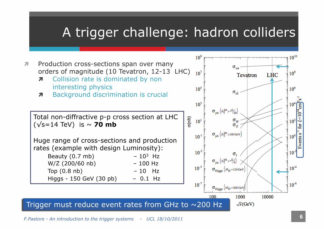
Production cross-sections span over many orders of magnitude (10 Tevatron, 12-13 LHC) Collision rate is dominated by non

interesting physics Background discrimination is crucial


Total non-diffractive p-p cross section at LHC (√s=14 TeV) is ~ 70 mb

Huge range of cross-sections and production rates (example with design Luminosity): Beauty (0.7 mb) – 103 Hz W/Z (200/60 nb) – 100 Hz Top (0.8 nb) – 10 Hz Higgs - 150 GeV (30 pb) – 0.1 Hz

Trigger must reduce event rates from GHz to ~200 Hz

Multi-purpose experiments: the trigger must satisfy a broad physics program, with no bias Main discovery channel (Higgs @LHC,

top @Tevatron), with precision EW Search for new phenomena Tests of pert-QCD, B physics….

Unlike e+e- colliders, each event contains more than one interaction, which add superimposed information on the detectors: pile-up “underlying events” from other partons in the same collision and

interactions from nearby bunch-crossings Detectors requirements The event characteristics vary with luminosity, not a simple events rescaling

but events with different number of muons, clusters,... affecting: the event-size, mainly with huge number of readout channels the trigger selection

…and more requirements


Inclusive selection

Flexible to cope changes in Luminosity and background

trigger requirements in HEP, i.e. what we want from the trigger?

Rate control = strong background rejection Instrumental or physics background Sometimes backgrounds have rates much larger than the signal

Need to identify characteristics which can suppress the background Need to demonstrate solid understanding of background rate and shapes

Maximize the collection of data for physics process of interest = high efficiency for benchmark physics processes ε trigger = Ngood (accepted)/Ngood (produced)


Not always both requirements can be realized: a compromise between number of processors working in parallel and fastness of the algorithms - to make it affordable

as selection criteria are tightened background rejection improves But selection efficiency decreases

Robustness of the selection is required, since discarded events are lost forever (reliable)

Different kind of triggers

Back-up triggers Back-up is misleading…. These triggers

are mandatory for most of the analysis Some large rate back-up triggers can

be pre-scaled

Pre-scaled triggers Only a fraction N of the events

satisfying the criteria is recorded. This is useful for collecting samples of high-rate triggers without swamping the DAQ system

Since trigger rate changes with Luminosity, dynamic pre-scales are sometimes used (reduce the pre-scales as Luminosity falls)


ATLAS L3 rate during a run

The bulk of the selected events are those useful for the physics analysis, but the trigger must also ensure rates for Instrumental and physics background studies Detector and trigger efficiency measurement from data Calibrations, tagging, energy scales…..

Minimum-bias triggers provide control triggers on the collision (soft QCD events), usually pre-scaled

The simplest trigger system Source: signals from Front-End electronics

Binary trackers (pixels, strips) Analog signals from trackers, time of light

detectors, calorimeters,….


source

trigger signal

The simplest trigger: apply a threshold Look at the signal Put a threshold as low as possible, since signals in HEP detectors have large amplitude variation Compromise between hit efficiency and noise rate

From Front-End Pre-amplifier Amplifier

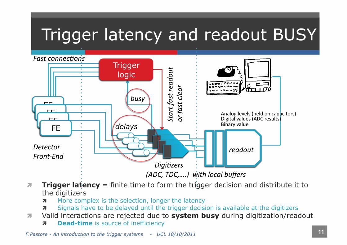
Trigger latency and readout BUSY

Trigger latency = finite time to form the trigger decision and distribute it to the digitizers More complex is the selection, longer the latency Signals have to be delayed until the trigger decision is available at the digitizers

Valid interactions are rejected due to system busy during digitization/readout Dead-time is source of inefficiency

FE FE FE FE

readout

Start fast reado

ut

or fa

st clear

Detector Front-‐End

Analog levels (held on capacitors) Digital values (ADC results) Binary value

busy

delays

Trigger logic

Fast connec5ons

Digi5zers (ADC, TDC,….) with local buffers


Trigger and data acquisition trends

As the data volumes and rates increase, new architectures need to be developed Allowed data bandwidth = Rate x Event size


Dead-time

The most important parameter controlling the design and performance of high speed DAQ systems Occurs whenever a given step in the processing takes a finite amount

of time It’s the fraction of the acquisition time in which no events can be

recorded, typically of the order of few %

Mainly three sources: Readout dead-time:

before the complete event has been readout, no other events can be processed (during this time the DAQ asserts a BUSY)

Trigger dead-time: trigger logic processing time, summed over all the components

Operational dead-time: data-taking runs


R RT

Raw trigger rate Read-out rate

Processing time

Td

Maximize event recording rate RT = raw trigger rate R = number of events read per second (DAQ rate) Td = dead time interval per event

fractional dead-time = R x Td live time = (1 - R x Td) number of events read: R = (1 - R x Td) x RT

The fraction of surviving events (lifetime ratio) is:

Td limits the maximum DAQ rate (R=1/Td)regardless of the trigger rate :

We always lose events if RT > 1/Td If exactly RT = 1/Td -> dead-time is 50%

Due to fluctuations, the incoming rate is higher than the processing one


R (H

z)

RT(Hz)

Td=1s

Td=2s

R RT Td

If readout-time is 1s, max rate is 1 Hz

The trick is to make both RT and Td as small as possible (R~RT)

Features to minimize dead-time

Two approaches are followed for large dataflow systems

Parallelism Independent readout and trigger processing paths, one for each

detector element Digitization and DAQ processed in parallel (as many as affordable!)

Pipeline processing to absorb fluctuations Organize process in different steps Use of local buffers (FIFOs) between steps allows steps with

different timing (big events processed during short events). The depth of local buffers limits the processing time of the

subsequent step: better if step3 is faster than step2

Segment as much as you can!


Buffering and filtering At each step, data volume is reduced, more refined filtering to the next step At each step, data are held in buffers

The input rate defines the processing time of the filter and its buffer size The output rate limits the maximum latency allowed in the next step Filter power is limited by the capacity of the next step

1

Filter step 1 Filter step 2

Max input rate Max output rate Max output rate Max input rate

Data volume reduces

As long as the buffers do not fill up (overflow), no additional dead-time is introduced!


If the rate after filtering is higher than the capacity of the next step Add filters (tighten the selection) Add better filters (more complex selections) Discard randomly (pre-scales)

Latest filter can have longer latency (more selective)

17 F.Pastore - An introduction to the trigger systems - UCL 18/10/2011 1

Filter step 1 Filter step 2

Max input rate Max output rate

Max output rate Max input rate

Data volume reduces

Rates and latencies are strongly connected

Multi-level triggers Adopted in large experiments, successively more complex decisions

are made on successively lower data rates First level with short latency, working at higher rates Higher levels apply further rejection power, with longer latency (more complex

algorithms)


Level-1 Level-2 Level-3

Exp. N.of Levels ATLAS 3 CMS 2 LHCb 3 ALICE 4

LHC experiments

Lower event rate Bigger event fragment size

More granularity information More complexity

Longer latency Bigger buffers

Efficiency for the desired physics must be kept high at all levels, since rejected events are lost for ever

Schema of a multi-level trigger @ colliders

In the collider experiments, the BC clock can be used as a pre-trigger First-level trigger (synchronous) can use the time between two BCs to

make its decision, without dead-time, if it’s long enough Fast electronics working at the BC frequency


First-level trigger

FE FE FE FE

readout Digi5zers (ADC, TDC,….) with local buffers

readout Detector Front-‐End

Fast connec5ons

High level trigger

busy

L1 Accep

t

BC clock

Logical division between levels

First-level: Rapid rejection of high-rate backgrounds Fast custom electronics processing fragments

of data from FE Coarse granularity data from detectors

Calorimeters for electrons/γ/jets, muon chambers Usually does not need to access data from the

tracking detectors (only if the rate can allow it) Needs high efficiency, but rejection power

can be comparatively modest

High-level: rejection with more complex algorithms Software selection, running on computer farms Progressive reduction in rate after each stage

allows use of more and more complex algorithms at affordable cost

Can access only part of the event or the full event (see next slides) Full-precision and full-granularity information Fast tracking in the inner detectors (for example to

distinguish e/γ)


Level-1

Level-2

Level-3

Level-1 trigger technologies

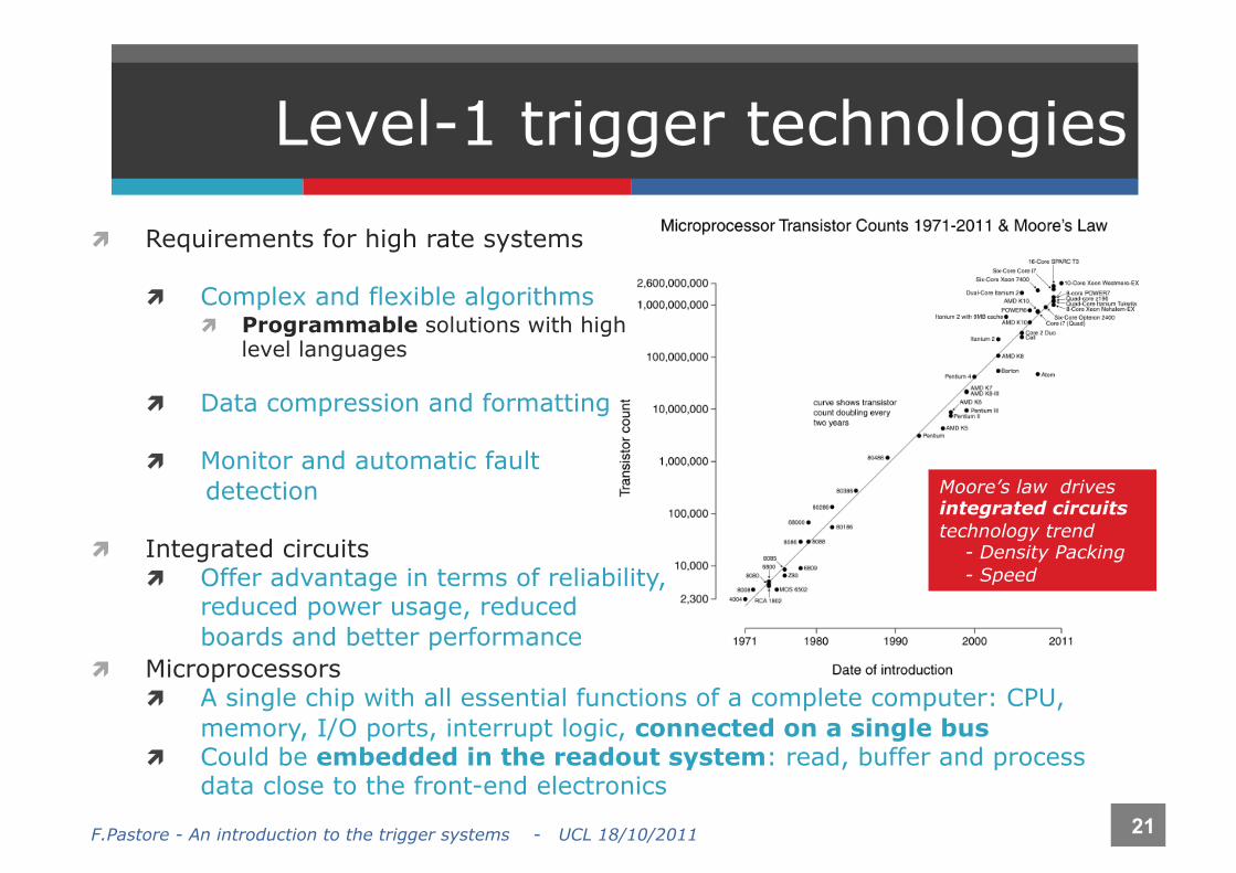
Requirements for high rate systems

Complex and flexible algorithms Programmable solutions with high

level languages

Data compression and formatting

Monitor and automatic fault detection

Integrated circuits Offer advantage in terms of reliability,

reduced power usage, reduced boards and better performance


Microprocessors A single chip with all essential functions of a complete computer: CPU,

memory, I/O ports, interrupt logic, connected on a single bus Could be embedded in the readout system: read, buffer and process

data close to the front-end electronics

Moore’s law drives integrated circuits technology trend - Density Packing - Speed

A trigger system can be made of different components Some elements have to be mounted on the detector (on-detector), some others can be placed into

crates with bus connections (off-detector)

High-speed serial links, electrical and optical, over a variety of distances Low cost and low-power LVDS links, @400 Mbit/s (up to 10 m) Optical GHz-links for longer distances (up to 100 m)

High density backplanes for data exchanges within crates High pin count, with point-to-point connections up to 160 Mbit/s Large boards preferred

Data movement technologies

On-‐detector

CMS first-level trigger

radiation tolerance cooling grounding operation in magnetic field very restricted access


Off-‐detector

HLT design principles Early rejection

Alternate steps of feature extraction with hypothesis testing: events can be rejected at any step with a complex algorithm scheduling

Event-level parallelism Process more events in parallel, with multiple processors Multi-processing or multi-threading Queuing of the shared memory buffer within processors

Algorithms are developed and optimized offline, often software is common to the offline reconstruction

P T T T

P P P P

Mul$-‐threading

Mul$-‐processing

I/O

I/O


High Level Trigger Architecture After the L1 selection, data rates are reduced, but can be still massive Key parameter for the design is the allowed bandwidth, given by average

event-size and trigger rate

LEP: 100 kByte event-size @ few Hz gives few 100 kByte/s Supported by 40 Mbyte/s VME bus

ATLAS/CMS: 1 MByte event-size @100 kHz gives ~100 GByte/s

Latest technologies in processing power, high-speed network interfaces, optical data transmission are used

High data rates are held by using

Network-based event building

Seeded reconstruction of data


N.Levels L1 rate (Hz)

Event size (Byte)

Readout bandw. (GB/s)

Filter out MB/s (Event/s)

ATLAS 3 L1: 105 106 10 ~100 (102)

L2: 103

CMS 2 105 106 100 ~100 (102)

Network-based HLT: CMS

Data from the readout system (RU) are transferred to the filters (FU) through a builder network

Each filter unit processes only a fraction of the events

Event-building is factorized into a number of slices, each one processing only 1/nth of the events

Large total bandwidth still required

No big central network switch Scalable

FU = several CPU cores = several filtering processes executed in parallel


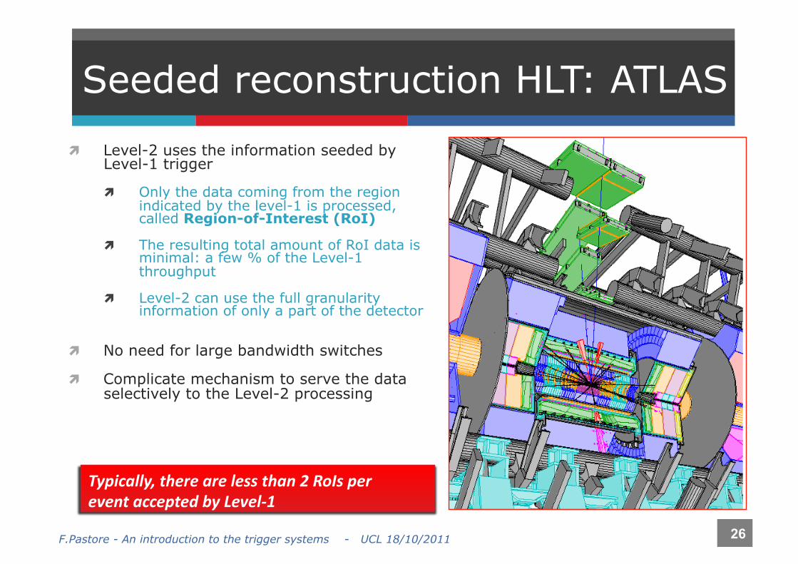
Seeded reconstruction HLT: ATLAS

Level-2 uses the information seeded by Level-1 trigger

Only the data coming from the region indicated by the level-1 is processed, called Region-of-Interest (RoI)

The resulting total amount of RoI data is minimal: a few % of the Level-1 throughput

Level-2 can use the full granularity information of only a part of the detector

No need for large bandwidth switches

Complicate mechanism to serve the data selectively to the Level-2 processing

Typically, there are less than 2 RoIs per event accepted by Level-‐1


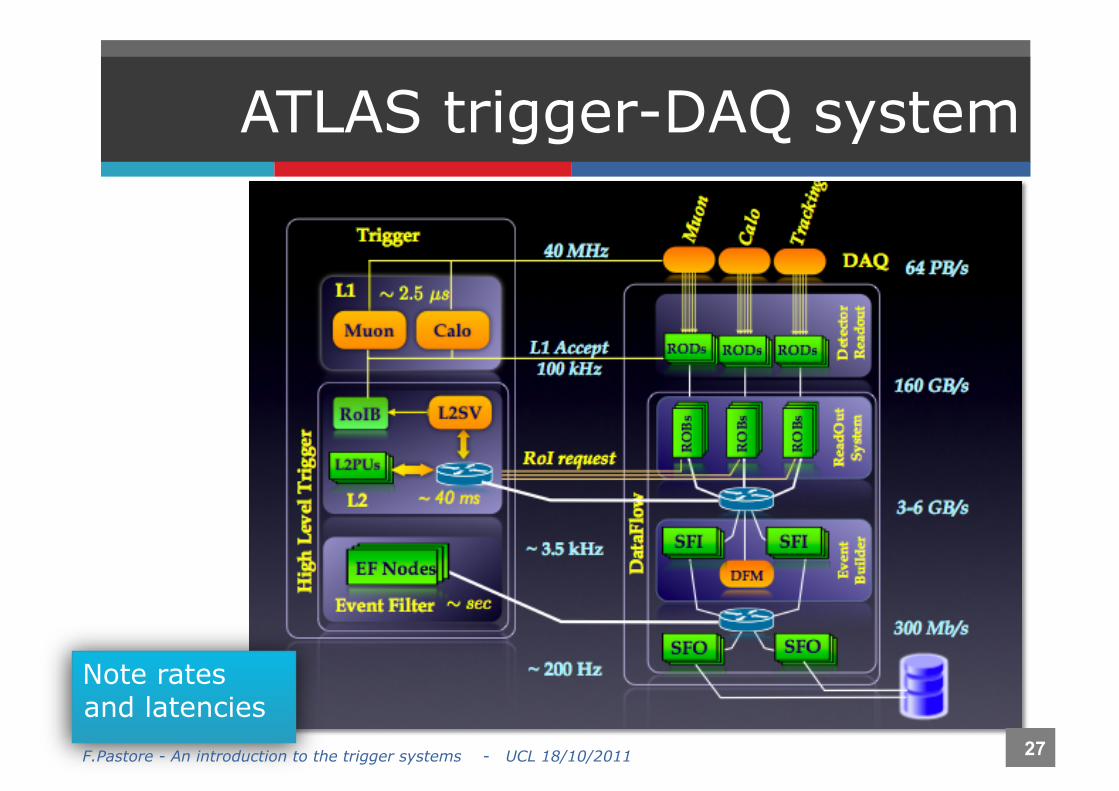
ATLAS trigger-DAQ system

Note rates and latencies


Trigger selections

Inclusive trigger

Confirm L1, inclusive and semi-incl., simple topology, vertex rec.

Confirm L2, more refined topology selection, near offline


Trigger signatures Signature=one or more parameters used for discrimination

Can be the amplitude of a signal passing a given threshold or a more complex quantity given by software calculation We first use intuitive criteria: fast and reliable Muon tracks, energy deposits in the calorimeters, tracks in the silicon

detectors….


Trigger selection is based on single/double particle signatures

Eventually combine more signals together following a certain trigger logic (AND/OR), giving redundancy Different signatures -> one analysis Different analysis -> one signature

Trigger criteria at colliders Apply thresholds on energy/momentum of the identified particles:

most used are electrons and muons which have clear signature

Shower shapes and isolation criteria are also used to separate single leptons from jets

In addition, global variables such as total energy, missing energy (for neutrino identification), back-to-back tracks, etc…


..and at hadron colliders Apply thresholds on transverse Energy (ET)

or transverse momentum (pT): component of energy or momentum orthogonal to the beam axis

Initial pT = 0 and Etotal < E 2 beams= Ecm

The bulk of the cross-sections from Standard Model processes are the presence of high-pT particles (hard processes)

In contrast most of the particles producing (minimum-bias) interactions are soft (pT ~ 1 GeV)

Large missing ET can be sign of new physics


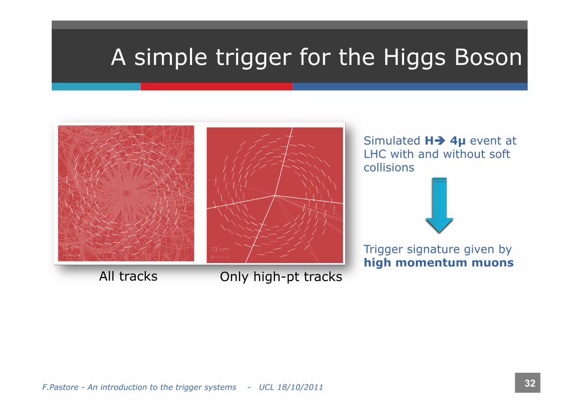
A simple trigger for the Higgs Boson

Simulated H 4µ event at LHC with and without soft collisions

Trigger signature given by high momentum muons


All tracks Only high-pt tracks

Example of multilevel trigger: ATLAS calorimeter trigger

e, γ, τ, jets, ETmiss, ΣET Various combinations of cluster sums

and isolation criteria Level-1

Dedicated processors apply the algorithms, using programmable ET thresholds

Peak finder for BC identification (signal is larger than 1 BC)

High-Level trigger Topological variables and tracking

information for electrons from Inner Detectors Cluster shape at L2 Jet algorithms at L3 (Event Filter)

Isolation criteria can be imposed to control the rate (reducing jet background at low energies thresholds)


Level-1 clustering algorithm

Cluster shape variable used in HLT for e/γ selection

Trigger efficiency as a parameter of your measurement

Efficiency should be precisely known, since it enters in the calculation of the cross-sections For some precise measurements, the crucial performance

parameter can be not the efficiency, but the systematic error in determining it

The orthogonality of the trigger requirements allows good cross-calibration of the efficiency

Signal


The trigger turn-on curves The capability of rate control (and bkg suppression) depends on the pT

(or ET) resolution Worst at level-1 (coarse granularity, δpT/pT up to 30%)

For example some particles can be under threshold, failing the trigger, because their pT is underestimated

Crucial is the study of the step region, in which efficiency changes very quickly and contamination from background is important (soft particles)


The dependency of ε on the true pT/ET, measured offline (with a resolution of order 0.1%) is described by the turn-on curves

ATLAS L1 MUON

Parametrizing the trigger efficiency

The trigger behavior, and thus the analysis sample, can change quickly due to important changes in Detector Trigger hardware Trigger algorithms Trigger definition

The analysis must keep track of all these changes

Multi-dimensional study of the efficiency: ε(pT, η, φ, run#) Fit the turn-on curves for different

bins of η, φ, Actually fit the 1/pT dependency

since the resolution is gaussian in 1/pT

CDF-Run II Fit of the muon trigger ε in bins of eta 36 F.Pastore - An introduction to the trigger systems - UCL 18/10/2011

Trigger efficiency measurement (1)

Basic idea: compare two cases in which the trigger selection is and is not applied It’s crucial to select the correct sample without biases

For HLT it’s easily done using back-up triggers called pass-through Do not apply the selection and calculate the denominator

Eff(L2MU10)= events passing L2MU10 events passing L2MU10_PASSTHROUGH


Efficiency = number of events that passed the selection number of events without that selection

For Level-1, we don’t know the absolute denominator Different methods can be used:

Compare independent (orthogonal) triggers (not correlated, min-bias) At the collider experiments can be measured with an experimental

technique called “Tag-and-Probe” (mainly lepton triggers)

Clean signal sample (Z, J/Ψ to leptons) Select track that triggered the event (Tag) Find the other offline track (Probe) Apply trigger selection on Probe

Helps in defining an unbiased sample (no background included)

Trigger efficiency measurement (2)


Use back-up triggers: L1_LOWEST_THRESHOLD

Efficiency = number of events that passed the selection number of events without that selection

Rates allocation of the trigger signatures

For design and commissioning, the trigger rates are calculated from large samples of simulated data, including large cross-section backgrounds 7 million of non-diffractive events @70mb

used for 1031 cm-2 s-1 in ALTAS Large uncertainties due to detector response and jet cross-sections: apply safety factors, then tuned with data

During running, extrapolation from data to higher Luminosity 39 F.Pastore - An introduction to the trigger systems - UCL 18/10/2011

Target is the final allowed bandwidth (~200 Hz @ LHC) Trigger rate allocation on each trigger item is based on

Physics goals (plus calibration, monitoring samples) Required efficiency and background rejection Bandwidth consumed

Rates scale linearly with luminosity, but linearity is smoothly broken due to pile-up

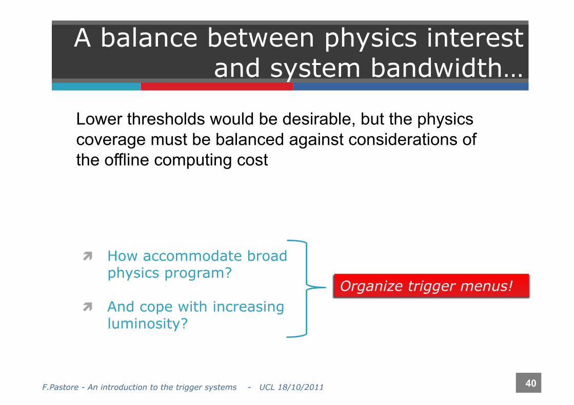
A balance between physics interest and system bandwidth…

How accommodate broad physics program?

And cope with increasing luminosity?


Organize trigger menus!

Lower thresholds would be desirable, but the physics coverage must be balanced against considerations of the offline computing cost

Design a trigger menu

A trigger menu is the list of our selection criteria Each item on the menu is a trigger chain

A trigger chain includes a set of cut-parameters or instructions from each trigger level (L1+L2+L3..)

Each chain has its own bandwidth allocation An event is stored if one or more trigger chain criteria

are met A well done trigger menu is crucial for the physics program

Multiple triggers serve the same analysis with different samples (going from the most inclusive to the most exclusive)

Ideally, will keep some events from all processes (to provide physics breadth and control samples)

The list must be Redundant to ensure the efficiency measurement Sufficiently flexible to face possible variations of the

environment (detectors, machine luminosity) and the physics program


A-tr

B-tr

My

mea

sure

C-tr

D-tr

E-tr

F-tr

Con

trol s

ampl

e

Trigger strategy @ colliders

Inclusive triggers designed to collect the signal samples (mostly un-prescaled) Single high-pT

e/µ/γ (pT>20 GeV) jets (pT>100 GeV)

Multi-object events e-e, e-µ, µ-µ, e-τ, e-γ, µ-γ,

etc… to further reduce the rate

Back-up triggers designed to spot problems, provide control samples (often pre-scaled) Jets (pT>8, 20, 50, 70 GeV) Inclusive leptons (pT > 4, 8 GeV) Lepton + jet


ATLAS

Example of trigger menu flexibility

ATLAS start-up L=1031 cm-2 s-1

Level-1: Low pT thresholds and loose selection criteria

In the meanwhile, deploy high thresholds and multi-objects triggers for validation (to be used as back-up triggers)

HLT: running in pass-through mode for offline validation or with low thresholds

Trigger menu evolved in several steps with LHC peak luminosity Complex signatures and higher pT

thresholds are added to reach the physics goals

Stable condition for important physics results (summer or winter conferences)

Mostly kept same balance between physics streams


Inclusive trigger example: from CDF

Level 1 EM Cluster ET > 8 GeV Rφ Track pT > 8 GeV

Level 2 EM Cluster ET > 16 GeV Matched Track pT > 8 GeV Hadronic / EM energy < 0.125

Level 3 EM Cluster ET > 18 GeV Matched Track pT > 9 GeV Shower profile consistent with e-


To efficiently collect W, Z, tt, tb, WW, WZ, ZZ, Wγ, Zγ, W’, Z’, etc…

Only one of these analysis needs to measure trigger efficiency, the others can benefit from one (use Standard Model Z,W)

Trigger Chain: Inclusive High-pT Central Electron

Back-up trigger example: from CDF

W_NOTRACK L1: EMET > 8 GeV && MET > 15 GeV L2: EMET > 16 GeV && MET > 15 GeV L3: EMET > 25 GeV && MET > 25 GeV

NO_L2 L1: EMET > 8 GeV && rφ Track pT > 8

GeV L2: AUTO_ACCEPT L3: EMET > 18 GeV && Track pT > 9 GeV

&& shower profile consistent with e- NO_L3

L1: EMET > 8 GeV && rφ Track pT > 8 GeV

L2: EMET > 8 GeV && Track pT > 8 GeV && Energy at Shower Max > 3 GeV

L3: AUTO_ACCEPT


Factorize efficiency into all the components:

efficiency for track and EM inputs determined separately separate contributions from all the trigger levels

Use resolution at L2/L3 to improve purity

only really care about L1 efficiency near L2 threshold

Back-up Triggers for central Electron 18 GeV:

Redundant trigger Example: from CDF

Inclusive, Redundant Inputs are helpful

L1_EM8_PT8 feeds Inclusive high-pT central electron

chains Di-lepton chains (ee, eµ, eτ) Several back-up triggers 15 separate L3 trigger chains in total

A ttbar cross section analysis uses Inclusive high-pT central e chains Inclusive high-pT forward e chains MET + jet chains Muon chains


Trigger menus must be

Inclusive: Reduce the overhead for the program analysis

Redundant: if there is a problem in one detector or in one trigger input, the physics is not affected (less efficiently, but still the measurement is possible)

Summarizing…. The trigger strategy is a trade-off between physics

requirements and affordable system power and technologies A good design is crucial – then the work to maintain optimal

performance is easy

Here we just reviewed the main trigger requirements coming from physics Design an architecture with low dead-time, in which each step of

the selection must accomplish requirements on speed and rate suppression

Perfect knowledge of the trigger selection on both signal and background

Flexibility and redundancy ensure a reliable system

In particular, for hadron colliders, like LHC, the trigger performance is crucial for discovery or not discovery new physics that can be easily lost if we don’t think of it in advance!


an introduction to the trigger systems - ucl hep...

Documents