An introduction to the simulation of fluid andstructure dynamics with emphasis on sport

applications

Luca Formaggia

MOX, Dipartimento di Matematica, Politecnico di Milanovia Bonardi 9, 20133 Milano, luca.formaggia@polimi.it

Computing and image processing with data related to humans andhuman activities

Outline

Introduction

Where mathematics meets sport

Fluid models – Navier-Stokes equations

Fluid models – Free surface flow

Structural Models

Coupled fluid-structure problem

Fluid equations in moving domains – ALE formulation

Algorithms for fluid-structure interaction with large displacements

Introduction

Where mathematics meets sport

Biomechanicsbiological response to fatigue

Injury/stress

Study of movement

Dynamical systemsContinuum mechanics

Strategy PlanningGame TheoryOperations Research

Optimization of sport devicesContinuum mechanicsScientific computingNumerical Analysis

In this lectures we focus on the last topic, and more precisely to fluid andstructure dynamics, as well as their coupling.

Optimization of rowing boats

The performance of a rowing boat is

strictly related (beside the ability of the

rowers) to the surface waves generated

during the motion (energy dissipated to

generate the waves + increased water re-

sistance)

More on the my next talk on Wednesday.

Optimization of sailing boats

The optimal design of a sailing yacht requires

a complex analysis of the fluid-dynamics

around the hull, keel and appendages, as well

as the interaction of the wind flow and sails.

Besides, studies are needed to assess stability

and maneuverability.

The study of optimal sail configura-tion and trimming require to solvea complex fluid-structure interactionproblem

More on the talk by Nicola Parolini next Monday.

Optimization swim suite and swimming style

The study of the movement of the arm during

swimming motion allows to assess the perfor-

mance of different styles and swimming tech-

niques.

The use of different fabric or seamsmay affect the resistance of a swimsuit

More on the talk by Edie Miglio next Tuesday.

Other examples

Computing the aerodynamics of a bobsleight

Simulating the trajectory of a soccer ball

Modeling the mechanics of golf swingaction

The fluid dynamics equations (Navier-Stokes)

Derivation of the Navier Stokes equationsLet’s consider a domain Ωf occupied by a fluid moving at velocityu(x, t), x ∈ Ωf , t > 0

Ω f

Trajectories of fluid particles:

x(t) : x(t) = u(x(t), t)

Given a scalar function f (x, t) (could be density, temperature, etc.), wecall material derivative its time variation along particle trajectories

Material derivative:Df

Dt(x, t) =

d

dtf (x(t), t)

Applying the usual chain rule we have

Df

Dt=

d

dtf (x(t), t) =

∂f

∂t+

3∑i=1

∂f

∂xi

∂xi∂t︸︷︷︸=ui

=∂f

∂t+ (u · ∇)f

Derivation of the Navier-Stokes equations

Consider now an arbitrary volume Vt transported by the fluid and a scalarquantity f (x, t) defined in Ωf

Ω f

n

Vt

Reynolds transport formula

d

dt

∫Vt

f dx =

∫Vt

∂f

∂tdx +

∫∂Vt

f u · n dA

=

∫Vt

(∂f

∂t+ div(f u)

)dx

Conservation of mass

Principle of mass conservation: given an arbitrary volume Vt moving withthe fluid, the mass contained in it will not change in time.

We denote by %f (x, t) the fluid density. Then

d

dt

∫Vt

%f dx = 0,by Reynolds thm

=⇒∫Vt

(∂%f∂t

+ div(%f u)

)dx = 0

Given the arbitrariness of the volume Vt , we conclude:

Mass conservation equation (or continuity eq.)

∂%f∂t

+ div(%f u) = 0, in Ωf , t > 0

Incompressibility assumption

I Many fluids (water or air at low velocity, for instance) can beconsidered incompressible.

I The incompressibility assumption is acceptable for Mach 1, wherethe Mach number is the ratio between the fluid velocity and thespeed of sound. (' 342 m/s in air, ' 1490 m/s in water)

In an incompressible fluid any arbitrary fluid subdomain Vt does notchange its volume

d

dt

∫Vt

1, dx = 0,by Reynolds thm

=⇒ div u = 0

In many practical cases (relevant for the class of problems we areconsidering) fluid can be considered a constant density fluid, whichimplies incompressibility.

Conservation of momentumPrinciple of momentum conservation (Newton’s second law): thevariation of the momentum equals the forces applied to the system

d

dt

∫Vt

%f u dx =

∫Vt

f dx +

∫∂Vt

t dA

ft

n

V t

where

I f are the external volume forces per unit volume (e.g. gravity∗%f )

I t are the internal surface tractions due to the interaction with thesurrounding fluid particles.

The Cauchy postulate asserts that t = t(x,n, t) depends only on theunit outward normal vector n to Vt in x.

The Cauchy theorem asserts that t depends linearly on n, i.e. thereexists a tensor σf , (called the Cauchy stress tensor), such thatt = σf · n.

Finally, σf is symmetric if no concentrated couples exist in the fluid(usually true for the target applications).

Conservation of momentumBy applying the Reynolds transport theorem + the divergence theorem +arbitrariness of Vt , we get

Momentum conservation equation (conservation form)

∂%f u

∂t+ div(%f u⊗ u)− div(σf ) = f, in Ωf , t > 0

Observe that

∂%f u

∂t+ div(%f u⊗ u) =

∂%f∂t

u + %f∂u

∂t+ %f u · ∇u + u div(%f u)

= u

(∂%f∂t

+ div(%f u)

)︸ ︷︷ ︸

=0(continuity eq.)

+%f

(∂u

∂t+ u · ∇u

)

Momentum conservation equation (Advective form)

%f

(∂u

∂t+ u · ∇u

)− div(σf ) = f, in Ωf , t > 0

Constitutive relations

To characterize a particular fluid, the Cauchy stress tensor has to berelated to the fluid motion

Newtonian fluid:

In a Newtonian fluid the Cauchy stress tensor is a function of a scalarvariable p called pressure and the strain tensor

D(u) =∇u +∇Tu

2

of the formσf (u, p) = −pI + 2µD(u) + λ(div u)I

where µ is the dynamic viscosity and λ the second coefficient of viscosity.For an incompressible Newtonian fluid

σf (u, p) = −pI + 2µD(u)

Navier-Stokes equations for constant density Newtonianfluids

%f(∂u

∂t+ u · ∇u

)− divσf (u, p) = f Momentum eqns.

div u = 0 Continuity equation

σf (u, p) = −pI + 2µD(u) D(u) =1

2(∇u +∇Tu)

Possible boundary conditions:

• imposed velocity profile: u = g on ΓD

• imposed traction σf · n = d on ΓN

• far field u = u∞ when x→∞

Example: flow around a ball

U I u = g on the ball (no-slip condition)

I u = U at far fieldThe value of g may derive from an interaction with the ball dynamics

Alternative formulations of momentum eqns

Conservative form

%f∂u

∂t+ div (%f u⊗ u− σf (u, p)) = f

Viscous term in Laplace form

Using the continuity equation, if µ is constant one may derive that

− divσf (u, p) = µ4u−∇p

This may lead to more efficient solution schemes, but is unsuitable forfluid structure algorithm since the associate natural boundary condition isnow

−pn + µ∇u · n 6= σf · n

is not identifiable anymore with the stress at the boundary.

Potential flows and Bernoulli lawWe consider an inviscid, incompressible fluid subject to conservativeforces f = ∇V (e.g. gravity: f = −ρf gez)

If the flow is initially irrotational, it will stay so for all times (Kelvintheorem)

Assume curl u = 0. Then, for a simply connected domain Ωf , there existsa potential φ such that u = ∇φ.

I Continuity eq.: div u = 0 =⇒ ∆φ = 0

I Momentum eq.: %f

(∂∇φ∂t + u · ∇u

)+∇p = ∇V

using the vector identity u · ∇u = 12∇|u|

2 − u×:0

curl u

=⇒ ∇(%f

∂φ∂t + %f

12 |u|

2 + p − V)

= 0

Bernoulli law %f∂φ

∂t+

1

2%f |u|2 + p − V = const

Potential equations∆φ = 0

p = c + V − %f(∂φ∂t + 1

2 |∇φ|2)

The effects of viscosityWhen considering the flow over a wall, the viscosity forces the fluidparticles to adhere to the wall −→ boundary layers effects. Let

I U: far field velocity; L: characteristic length of the wallI Re = %f UL/µ: Reynolds number; measures the relative importance

of inertia effects (U ∗ L) versus viscous effects (µ/%f ).

Flow over a flat wall (∂xp = 0)

I boundary layer of thickness z =√

LxRe

(increasing along the wall – Blasiussolution)

I shear forces (drag) on the wall(σf · n) · ex ≈ µ∂ux∂z

x

y

zslope ~

drag forces

Flow over a curved wall

I The pressure gradient along the wallcauses the fluid to separate from thewall. This is at the basis of the wellknown Von Karman vortex sheddingphenomenon

What gives the lift?

It is known that if we spin a ball (soccer, golf, tennis,...) while moving weare able to make it turn.The phenomenon may explained in a simple way with a 2D example andpotential theory (yet accurate 3D computations may be complex)

F

tU

x

y

u<U

u>U

(larger pressure)

(smaller pressure)

The spin induces an irrotationalvortex which superimposes to thefree stream velocity U causing adifference of pressure thanks toBernoulli’s law.

F = −ρf ΓUey

where Γ is the circulation of u

Γ =

∮u · tdγ

Turbulence

The Navier-Stokes equations becomeunstable when the transport term (u · ∇u)is dominant with respect to the viscousterm (2µD(u)), i.e. when Re 1.

In such a situation, energy is transferred from large eddies (large vortexstructures) to smaller ones up to a characteristic scale, so calledKolmogorov scale where they are dissipated by viscous forces.

Kolmogorov scale lK ∼ L ∗ Re−3/4

A direct numerical simulation (DNS) aims at simulating all relevant scalesup to the Kolmogorov scale. Therefore, the mesh size has to be h ≈ lK .

3D simulations #Dofs ∼(

L

h

)3

∼ Re9/4

Unfeasible even for nowadays computers for Re ∼ 104 ÷ 106.

Kinetic energy decayIt is instructive to look at the fluid kinetic energy E = 1

2%f |u|2 and

perform a Fourier analysis with respect to space wavenumbers:

E (k) =

∫S(k)

∫R3

E (x)e ix·k dx dA, with S(k) = |k| = k

E(k) = c k kε 2/3

−5/3

log E

(k)

log(k)L−1

l k−1

tranfer of energyproduction

of energy of energydissipation

(integral scale) (Kolmogorov scale)

inertial region

The decay E (k) ∼ ε2/3k−5/3 is one of the main results of Kolmogorovtheory of turbulence, valid for homogeneous isotropic turbulence

Turbulence and boundary layer

The golf ball

The roughness of a golf ballenergizes the boundary layerretarding flow separation.The Pressure induced drag isthen reduced. Even if viscousdrag is likely to be greaterthan that on a smooth ballthe overall resistance isdiminished.

Turbulence and boundary layer

Laminar turbulent transition

As the boundary layer grows even aninitially laminar flow (i.e. with noturbulence) will become turbulent. Thepoint where this change of behavior occursis called laminar-turbulent transition point.

The location of the Laminar-turbulenttransition is very important to determinethe drag of submerged bodies like a yachtbulb, since it affects the resistance.Mathematical models of the transition arestill a partially open problem.

The level of simulation of turbulent flows

I Direct NS simulation Used only for special studies. In general isunfeasible

I Large Eddy Simulation We model only the smallest scale turbulence.Rather costly for high Reynolds.

I Differential Models. Based on the Raynolds averaging paradigmwhere turbulence is accounted for by modifying the viscosityµ→ µ+ µt . We add advection-diffusion-reaction equations forquantities like the turbulence kinetic energy (κ) and dissipation (ε)and µt = µt(κ, ε). They need several empirical closure relation.Most used in engineering applications. Often indicated as RANS(Reynolds Averaged Navier Stokes).

I Algebraic models Also based on RANS. We use algebraic relations tolink µt to the mean flow velocity. Applicable only to attached flowand special geometries.

Numerical approximation of theNavier-Stokes equations

Finite Volumes

They are based on the equations written in conservative form

∂u

∂t+ div F(u, p) = S

The domain is subdivided into a mesh of polygons (finite volumes, alsocalled control volume) Ci , i = 1, ...N.

By applying the divergence theorem

d

dt

∫Ci

u(t) +

∫∂Ci

F(u(t), p(t)) · ndγ =

∫Ci

S(t)

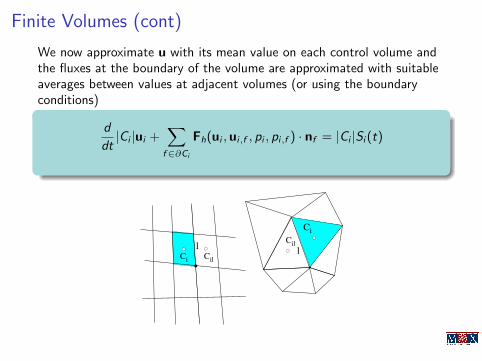
Finite Volumes (cont)

We now approximate u with its mean value on each control volume andthe fluxes at the boundary of the volume are approximated with suitableaverages between values at adjacent volumes (or using the boundaryconditions)

d

dt|Ci |ui +

∑f∈∂Ci

Fh(ui ,ui,f , pi , pi,f ) · nf = |Ci |Si (t)

Cil

Ci

Cil

C

ll

i

Finite element approximation of the Navier-Stokesequations

We will consider only flows in laminar regimes (no turbulence models)

Navier-Stokes equations

%f∂u

∂t+ %f u · ∇u− divσf (u, p) = f f , in Ω, t > 0,

div u = 0, in Ω, t > 0,

u = g, on ΓD , t > 0,

σf · n = d, on ΓN , t > 0,

u = u0, in Ω, t = 0

with σf (u, p) = 2µD(u)− pI

Weak formulationLet us define the following functional spaces:

V = [H1(Ω)]d V0 = [H1ΓD

(Ω)]d ≡ v ∈ V, v = 0 on ΓDQ = L2(Ω)

Remark: if ΓD = ∂Ω, the pressure is defined only up to a constant. Thepressure space should be Q = L2(Ω) \ R.

We multiply the continuity equation by a test function q ∈ Q and themomentum equation by a test function v ∈ V0 and integrate over thedomain.

Integration by parts of the stress term:∫Ω

− divσf · v =

∫Ω

σf : ∇v −∫∂Ω

(σf · n) · v

=

∫Ω

2µD(u) : ∇v −∫

Ω

pI : ∇v︸ ︷︷ ︸=p div v

−

*0∫

ΓD

(σf · n) · v −∫

ΓN

(σf · n︸ ︷︷ ︸=d

) · v

Weak formulation

Navier Stokes equations – weak formulation

Find (u(t), p(t)) ∈ V × Q, u(0) = u0, u(t) = g(t) on ΓD such that∫Ω

%f

(∂u

∂t+ u · ∇u

)· v +

∫Ω

2µD(u) : ∇v −∫

Ω

p div v =

∫Ω

f · v +

∫ΓN

d · v∫Ω

q div u = 0

∀(v, q) ∈ V0 × Q

Weak solutions exist for all time ([Leray ’34], [Hopf ’51]). Uniqueness isan open issue in 3D.

Finite element approximationIntroduce finite dimensional spaces of finite element type

Vh ⊂ V; Vh0 = Vh ∩ V0; Qh ⊂ Q

Observe that pressure functions need not be continuous.

Moreover let us denote by uh0 ∈ Vh and gh ∈ Vh(ΓD) suitableapproximations of the initial datum and Dirichlet boundary datum

Finite Element approximation (continuous in time)

Find (uh(t), ph(t)) ∈ Vh × Qh, uh(0) = uh0, uh(t) = gh(t) on ΓD such that∫Ω

%f

(∂uh

∂t+ uh · ∇uh

)· v +

∫Ω

2µD(uh) : ∇v −∫

Ω

ph div v

=

∫Ω

f · v +

∫ΓN

d · v∫Ω

q div uh = 0

∀(v, q) ∈ Vh0 × Qh

Algebraic formulationI φi

Nu

i=1: basis of Vh0

I φ(b)j

Nbu

j=1: basis of Vh \ Vh0 (shape functionscorresponding to boundary nodes)

I ψlNp

l=1: basis of Qh

φ j(b)

ψl

φ i

Expand the solution (uh(t), ph(t)) on the finite element basis

uh(x, t) =Nu∑i=1

ui (t)φi (x) +

Nbu∑

j=1

gi (t)φ(b)j (x)︸ ︷︷ ︸

=gh known term

ph(x, t) =

Np∑l=1

pi (t)ψl(x)

Vectors of unknown dofs (nodal values if Lagrange basis functions areused)

U(t) = [u1(t), . . . , uNu (t)]T , P(t) = [p1(t), . . . , pNp (t)]T

Algebraic systemReplacing in the Galerkin formulation the expansions of uh and ph on thefinite element basis and testing with shape functions φi and ψl we are ledto the following system of ODEsM

dU

dt+ AU + N(U)U + BTP = Fu(U),

BU = Fp,t > 0

with

Mij =

∫Ω

%fφjφi mass matrix Aij =

∫Ω

2µD(φj) : ∇φi , stiffness matrix

N(U)ij =

∫Ω

uh · ∇φj · φi , !! depends on U; non linear term

Bli = −∫

Ω

ψl divφi , divergence matrix

(Fu(U))i =

∫Ω

f · φi +

∫ΓN

d · φi −∫

Ω

%f

(∂gh

∂t+ uh · ∇gh

)· φi −

∫Ω

2µD(gh) : ∇φi

(Fp)l =

∫Ω

div gh ψl

A simpler problem – Stokes equationLet us consider for the moment the steady state Stokes problem

−2µ div D(u) +∇p = f, in Ω,

div u = 0, in Ω,

u = g, on ΓD ,

(2µD(u)− pI) · n = d, on ΓN ,

Weak formulation: find (u, p) ∈ [H1]d × L2, u = g on ΓD , such thata(u, v) + b(v, p) = F(v), ∀v ∈ [H1

ΓD]d

b(u, q) = 0, ∀q ∈ L2

with

a(u, v) =

∫Ω

2µD(u) : ∇v, b(v, p) = −∫

Ω

p div v,

F(v) =

∫Ω

f · v +

∫ΓN

d · v

Stokes problemThe Stokes problem is well posed (admits a unique solution (u, p) whichdepends continuously on the data).

In particular, the bilinear form b(·, ·) satisfies the important property(LBB condition)

infq∈L2

supv∈H1

ΓD

b(v, q)

‖v‖H1‖q‖L2

≥ β > 0

which implies that ∀q ∈ L2, ∃vq ∈ H1ΓD

: b(vq, q) > 0.

Finite elements approximation: find (uh, ph) ∈ Vh × Qh, uh = gh on ΓD ,such that

a(uh, vh) + b(vh, ph) = F(vh), ∀vh ∈ Vh,0

b(uh, qh) = 0, ∀q ∈ Qh

(*)

Corresponding algebraic formulationAU + BTP = Fu

BU = Fp

=⇒[

A BT

B 0

] [UP

]=

[Fu

Fp

]The algebraic system has the typical structure of a saddle point problem

Spurious pressure modesIf these exists a pressure p∗h such that

b(vh, p∗h) = 0, ∀vh ∈ Vh,

this pressure will not be seen by the first equation of (*). It follows that,if (uh, ph) is a solution of (*), then also (uh, ph + p∗h) is a solution to thesystem and we loose uniqueness of the pressure.

Such a pressure p∗h is called a spurious pressure mode

A necessary and sufficient condition to avoid the presence of spuriouspressure modes is that the finite elements spaces Vh × Qh satisfy the

inf-sup condition: infqh∈Qh

supvh∈Vh0

b(vh, qh)

‖vh‖H1‖qh‖L2

≥ βh > 0

Observe that the inf-sup condition is satified by the continuous spacesV0 × Q but not necessarily by the finite element spacese Vh,0 ⊂ V0 andQh ⊂ Q.

At the algebraic level, the inf-sup condition is equivalent to the requestthat Ker(BT ) = ∅

Spurious pressure modesSpaces that satisfy the inf-sup condition are called compatible.

Assume the spaces (Vh,0,Qh) are compatible with a constant βhindependent of h. Then, the optimality of the Galerkin projection holds:

‖uh−uex‖H1 +‖ph−pex‖L2 ≤ C

(inf

vh∈Vh

‖uex − vh‖H1 + infqh∈Qh

‖pex − qh‖L2

)

Examples of spaces that satisfy the inf-sup condition

P2 /P1 Pbubble1 /P1 Q2 /Q1

Examples of spaces that do not satisfy the inf-sup condition

P1 /P1 P1 /P0 Q1 /Q1

Examples of spurious modes

Couette flow:

exact solution: u1 = y ; u2 = p = 0 .n=

0σ

.n=

0σ

u=1

u=0

IsoValue-9.94024-8.52021-7.57352-6.62683-5.68015-4.73346-3.78677-2.84008-1.8934-0.94671-2.32106e-050.9466641.893352.840043.786734.733415.68016.626797.573479.94019

Pressure

Pressure computed with P1/P0

IsoValue-3.7491-3.21351-2.85645-2.4994-2.14234-1.78528-1.42822-1.07116-0.714103-0.3570451.34456e-050.3570720.714131.071191.428251.785312.142362.499422.856483.74913

Pressure

Pressure computed with P1/P1

The issue of spurious pressure modes appears in the full Navier-Stokesequations as well. It is related to the incompressibility contraint.

Back to the Navier-Stokes equations: Temporaldiscretization

A simple time integration scheme: Implicit Euler with semi-implicittreatment of the convective term:%f

un − un−1

∆t+ un−1 · ∇un − div(2µD(un)) +∇pn = fn

div un = 0

in Ω, n = 1, 2, . . .

u0 = u0, un = gn on ΓD − pnn + 2µD(un) · n = dn on ΓN

In algebraic form this leads to a linear system to solve at every time step,of the form[

1∆t M + A + N(Un−1) BT

B 0

][Un

Pn

]=

[Fnu + 1

∆t MUn−1

Fnp

]

Observe the structure of the matrix, equal to the one for the Stokesproblem.

Projection methodsThe idea of projection methods is to avoid the costly solution of thesaddle point problem and to split the computation of velocity andpressure at each time step.

Fractional step approach (assume homogeneous Dirichlet boundary cond.)

NS eqs. %f∂u

∂t+ L1u︸︷︷︸

viscous+transport terms

+ L2u︸︷︷︸incompress. constraint

= f

Split the computation into

Step I:

%fun − un−1

∆t+ L1un = fn

un|∂Ω = 0(transport-diffusion eq.)

Step II:

%f

un − un

∆t+∇pn = 0

div un = 0

un|∂Ω · n = 0

(L2-proj. on divergencefree functions)

Some numerical issues

I High Reynolds flow may need stabilization of the convective term toavoid spurious oscillations in the velocity

I Non-conforming discretization may be computationally attractive ⇒stabilized schemes to circumvent the LBB condition

I The numerical problem is usually quite large (> 106 unknown). Aniterative solution of the linear system is mandatory → goodpreconditioners are required

I To afford large computation in acceptable times we need parallelcomputing (and parallel, scalable preconditioners as well)

I Turbulence modeling is still an active research problem

Some references on the Navier-Stokes problemA.J. Chorin, J.E. Marsden. A mathematical introduction to fluid mechanics.Third edition. Springer-Verlag, 1993

H. Elman, D. Silvester, A. Wathen. Finite elements and fast iterative solvers:with applications in incompressible fluid dynamics. Oxford University Press,2005

J.H. Ferziger, M. Peric, Computational Methods for Fluid Dynamics, Springer,2002

J.L. Geurmond, P. Minev, J. Shen An overview of projection methods for

incompressible flows, Comput. Methods Appl. Mech. Engrg. 195 (2006)

60116045

P.M. Gresho, R.L. Sani. Incompressible Flow and the Finite ElementMethod. (Two volumes), Wiley, 2000.

W. Layton. Introduction to the numerical analysis of incompressibleviscous flows. Society for Industrial and Applied Mathematics (SIAM),2008.

A. Prohl Projection and quasi-compressibility methods for solving theincompressible Navier-Stokes equations. B.G. Teubner, 1997

A. Quarteroni. Numerical models for differential problems.Springer-Verlag, 2009.

Free surface flow

Free Surface Flow

Γ

Γ

Γ

open

s

b

c

γ

Γ

fo

We consider a fluid domain composed by

I the bottom surface Γb(t) = (x , y ,−h(t))|(x , y) ∈ ΩI the free surface Γs(t) = (x , y , η(t))|(x , y) ∈ ΩI the lateral boundary Γl(t) = (x , y , z)|(x , y) ∈ γf , z ∈ (−h, η(t)).

The Navier-Stokes equations (revisited)

Du

Dt= −1

ρ

∂p

∂x+∇ · (ν∇u) +

∂

∂z

(ν∂u

∂z

)+ fv ,

Dv

Dt= −1

ρ

∂p

∂y+∇ · (ν∇v) +

∂

∂z

(ν∂v

∂z

)− fu,

Dw

Dt= −1

ρ

∂p

∂z+∇ · (ν∇w) +

∂

∂z

(ν∂w

∂z

)− g ,

∂u

∂x+∂v

∂y+∂w

∂z= 0,

I ∇ is the 2D Laplace operator (while ∇ is the 3D operator);

I ν is the kinematic viscosity coefficient, ν = µ/ρ

I f the Coriolis coefficient

I D/Dt = ∂/∂t + u · ∇

Mathematical models

Traditionally methods used for free surface dynamics fall into one ofthese categories

Integral equations boundary elements orpanel methods.

Interface capturing methods Volume offluid. MAC methods. We solve theequations for both water and air. We canaccount for overturning and breaking waves.

Interface tracking methods. The surface isdescribed by a function η = η(x , y , t). Weneed to solve the equation only for thewater, but we cannot describe overturningwaves

The VOF method

The domain Ω comprised both water and air. The interface is tracked bymeans of an additional scalar variable c which is transported with thefluid

∂c

∂t+ (u · ∇)c = 0 in Ω

with initial datum

c =

1 in water

0 in air

Thenρ = cρw + (1− c)ρair µ = cµw + (1− c)µair

Remark: Care must be taken in the discretization of the transportequation to avoid excessive “smearing” of the interface.

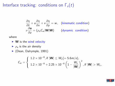
Interface tracking: conditions on Γs(t)

∂η

∂t+ u

∂η

∂x+ v

∂η

∂y= w , (kinematic condition)

ν∂u

∂z= (ρaCw |W|W) (dynamic condition)

where

I W is the wind velocity

I ρa is the air density

I (Dean, Dalrymple, 1991)

Cw =

1.2× 10−6, if |W| ≤Wc(= 5.6m/s),

1.2× 10−6 + 2.25× 10−6

(1− Wc

|W|

)2

, if |W| > Wc ,

Conditions on Γb (fixed bottom) and Γl

u∂h

∂x+ v

∂h

∂y+ w = 0 (kinematic condition)

ν∂u

∂z= f2(u), (dynamic condition)

The function f2 accounts for the friction on the bottom and may take asimilar form to that used on the free surface. It approximates the actionof the boundary layer at the bottom that in this type of formulation isusually not resolved.On Γl we may have any admissible condition for a Navier-Stokes problem.However, computationally it may be convenient to devise non reflectiveconditions for the elevation.

Integral form of the free surface equation

We integrate the continuity equation along the vertical coordinate∫ η

−h

∂u

∂xdz +

∫ η

−h

∂v

∂ydz + w |Γs = 0

Using the kinematic condition at free surface ⇒

∂η

∂t+

∂

∂x

∫ η

−hudz +

∂

∂y

∫ η

−hvdz = 0

Remark: the free surface is represented by a single valued function of xand y and t: no overturning or breaking waves are allowed in thisformulation.

The non-hydrostatic model

We split the pressure into a constant term (atmospheric pressure, may beset to zero) a hydrostatic component and a non-hydrostatic correction

p = pa + ρg(η − z) + gq.

Du

Dt−∇ · (ν∇u)− ∂

∂z

(ν∂u

∂z

)+∇q + g∇η = f

Dw

Dt−∇ · (ν∇w)− ∂

∂z

(ν∂w

∂z

)+∂q

∂z= 0,

∇ · u +∂w

∂z= 0

∂η

∂t+∇ ·

∫ η

−hudz = 0

When the ratio between basin height and wave length H/L << 1horizontal viscous term are small compared to the vertical ones (Greneret al 2000), so may be neglected.

The 2D equivalent: Boussinesq equations

With certain manipulations a 2D approximation may be devised:

∂η

∂t+∇ · [(η + h)u] = 0,

∂u

∂t+ u · ∇u + g∇η =

h

2∇∇ · (h

∂u

∂t)− h2

6∇∇ · ∂u

∂t,

Eliminating the terms in blue we obtain the shallow water equations.Pressure is recovered via Bernoulli’s relation

p = gρ(η − z) +ρ

2(2hz + z2)∇ · ∂u

∂t.

Remark: However, for boat dynamics the 2D equations are inadequate.

Waves produced by a ship in a channel

Hydrostatic case

Non hydrostaticcase

Lagrangian treatment of time derivative

We use the approximationDu

Dt(tn+1) ' un+1 − un(X)

∆twhere the foot of

the characteristic line X(s; t, x) is obtained by solving an ODE

dX(s; t, x)

ds= V(s,X(s; t, x)) for s ∈ (0, t),

X(t; t, x) = x.

Discretization: backward (composite) Euler (other possibility:Runge-Kutta scheme)

.X

x.

.

..

.

.

Care must be taken if X falls outside the domain.

How to account for the presence of the boat?

A possibility is to describe the boat external shape by means of a suitablefunction Ψ = Ψ(x , y , t) and impose that η ≤ Ψ at all times.

η

Ψ

ω γΨ

Some References on free-surface and ship hydrodynamics

R. Azcueta. Computation of turbulent free-surface flows around ships andfloating bodies. Ship Technology Research, 49(2):4669, 2002

U. Bulgarelli, C. Lugni, M. Landrini. Numerical modelling of free-surface flowsin ship hydrodynamicsInt. J. Numer. Meth. Fluids, 43(5):465-481, 2003.

C.C. Mei. The applied dynamics of ocean surface waves. World ScientificPublishing, Singapore, 1989

E. Miglio and A. Quarteroni. Finite element approximation of Quasi-3D shallowwater equations. Comput. Methods Appl. Mech. Engrg. 174(3-4):355-369 ,1999

N. Parolini and A. Quarteroni. Mathematical models and numerical simulationsfor the Americas Cup Comput. Methods Appl. Mech. Engrg.194(9-11):1001-1026, 2005

G. B. Witham. Linear and non linear waves, Wiley, 1974

Structural models and their finite elementapproximation

Structural models – kinematicsDynamics of structures is more conveniently described in Lagrangiancoordinates, i.e. equations are written in the reference configuration Ωs

0

(e.g. the initial configuration).

Lagrangian map: x = x(ξ, t) = Lt(ξ)

I ξ: coordinate of material pointin reference configuration

I x: coordinate of material pointin deformed configuration

I η(ξ, t) = x− ξ displacement ofmaterial point

η= −ξx Ω

s

tΩs

0

ξ

x

Kinematics

velocity : u(ξ, t) =∂x

∂t(ξ, t) = x(ξ, t) = η(ξ, t)

acceleration : a(ξ, t) =∂2x

∂t2(ξ, t) = x(ξ, t) = η(ξ, t)

Eulerian versus Lagrangian

Lagrangian frame (mostly used for solids)

Kinematics is described in the reference configuration

position x = x(ξ, t)velocity u = u(ξ, t) = x(ξ, t)acceleration a = a(ξ, t) = x(ξ, t)

Eulerian frame (mostly used for fluids)

Kinematics is described in the current (deformed) configuration

position (trajectories) x(ξ, t) : x = u(x, t), x(ξ, 0) = ξvelocity u = u(x, t)acceleration a = a(x, t) = Du

Dt (x, t) = ∂u∂t + u · ∇xu

Measures of strainLet us introduce the deformation gradient tensor

F = ∇ξx = I +∇ξη Fij =∂xi∂ξj

Given an infinitesimal material line segment dξ in Ωs0, it will be

transformed through the Lagrangian map into dx = Fdξ.

I Right Cauchy-Green tensor C = FTFMeasures the change in ‖dξ‖ due to the motion.

‖dx‖2

‖dξ‖2=

dxT·dx

‖dξ‖2=

dξTFTFdξ

‖dξ‖2=

dξT

‖dξ‖C

dξ

‖dξ‖= vTCv = λ2(v)

with v = dξ/‖dξ‖ unitary vector.

The change in length of dξdepends on its orientation.

x=x( ,t)ξ

(v)||d ||ξλ

Ω0

s

Ω0

sΩ

t

s

v||d ||ξ

Equations of motion

Equations in the reference configuration (Vt is a materal volume)

Id

dt

∫Vt

%su dx =d

dt

∫V0

J%s︸︷︷︸%0s

u dξ =

∫V0

%0sa dξ =

∫V0

%0s η dξ

I

∫Vt

f dx =

∫V0

J(ξ)f(x(ξ, t))︸ ︷︷ ︸f0(ξ)

dξ

I ∫∂Vt

tdA =

∫∂Vt

σsndANanson’s f.

=

∫∂V0

JσsF−T︸ ︷︷ ︸

σ0s

n0dA0 =

∫V0

divξ σ0s dξ

momentum equation %0s η − divξ σ

0s = f0

where we have introduced the first Piola-Kirchhoff stress tensor (alsocalled nominal stress tensor) σ0

s = JσsF−T . Observe that the divergencedivξ is taken with respect to the reference coordinate ξ.

Constitutive relations

Differently than for fluids, in an elastic body the internal stress dependson of deformation gradients (instead of gradients of deformation rates).

Cauchy elastic material

I σ0s is a continuous function of F =⇒ σ0

s = σ0s (F)

I Frame indifference =⇒ σ0s (QF) = σ0

s (F)QT for all Q orthogonal.Implies that σ0

s can be expressed as a funtion of C = FTF only:σ0

s = σ0s (C)

I Incompressible materials: one adds the constraint det F = 1 and acorresponding pressure p (Lagrange multiplier)

σs = σs(η)− pI, =⇒ σ0s = σ0

s − pJF−T

Examples of constitutive relations

Incompressible materials (J = 1)

I Neo-Hookean: W (C) = µ2 (tr C− 3)

σ0s = 2F

∂W

∂C− pJF−T = µF− p Cof F

I Mooney-Rivlin: W (C) = µ1

2 (tr C− 3)− µ2

2 (I2(C)− 3)

σ0s = 2F

∂W

∂C− pJF−T =

(µ1 + µ2 tr(FTF)

)F− µ2FFTF− p Cof F

Compressible materialsI Saint-Venant Kirchhoff: W (C) = λ

2 tr(E)2 + µ tr(E2)with E = 1

2 (C− I) and (λ, µ) Lame constants

σ0s = 2F

∂W

∂C= F

∂W

∂E= F (λ(tr E)I + 2µE)

Equations of elasto-dynamicsCompressible materials

%0s η − divξ σ

0s (η) = f0, σ0

s = 2F∂W

∂C

Incompressible materials%0s η − divξ σ

0s (η, p) = f0, σ0

s = 2F∂W∂C − p Cof F

J = 1

Possible boundary conditions

I imposed displacement: η = g on ΓD

I imposed nominal stress: σ0sn0 = d on ΓN

Example: incompressible Neo-Hookean material%0s η − divξ [µF(η)− p Cof F(η)] = f0(η) in Ω0

s

J(η) = 1 in Ω0s

η = g on ΓD

σ0sn0 = d on ΓN

Finite element approximation – compressible caseConsider a finite element space Vh ⊂ V (e.g. piecewise continuouspolynomials) defined on a suitable triangulation Th of Ωs

0.

Finite element formulation: find ηh(t) ∈ Vh, ηh = gh on ΓD , such that

∫Ωs

0

%0s

∂2ηh

∂t2· φh +

∫Ωs

0

σ0s (ηh) : ∇ξφh =

∫Ωs

0

fs0 · φh +

∫ΓN

d · φh dA0

for all φh ∈ Vh, vanishing on ΓD

Introduce a basis φiNs

i=1 of Vh and expand the displacement ηh on the

basis: ηh(t, ξ) =∑Ns

i=1 ηi (t)φi (ξ).

Then, we obtain a system of non-linear ODEs

Ms ds + Ks(ds) = Fs , t > 0 (1)

withI Solution vector: ds(t) = [η1(t), . . . ,ηNs

(t)]T

I Mass matrix: (Ms)ij =∫

Ωs0%0sφiφj

I Stiffness (nonlinear) term: (Ks(ds))i =∫

Ωs0σ0

s (ηh) : ∇ξφi

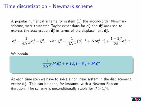
Time discretization - Newmark scheme

A popular numerical scheme for system (1) the second-order Newmarkscheme, were truncated Taylor expansions for dn

s and dns are used to

express the acceleration dns in terms of the displacement dn

s .

dns =

1

β∆t2dns − ζ

n, with ζn =1

β∆t2(dn−1

s + ∆tdn−1s ) +

1− 2β

2βdn−1s

We obtain

1

β∆t2Msd

ns + Ks(dn

s ) = Fns + Msζ

n

At each time step we have to solve a nonlinear system in the displacementvector dn

s . This can be done, for instance, with a Newton-Rapsoniteration. The scheme is unconditionally stable for β > 1/4.

Some references on elasticity and its numericalapproximation

J. Bonet, R.D. Wood. Nonlinear continuum mechanics for finite elementanalysis. Second edition. Cambridge University Press, 2008.

T. Belytschko, W.K. Liu, B. Moran. Nonlinear finite elements for continua andstructures. John Wiley & Sons, Ltd., Chichester, 2000.

P.G. Ciarlet Mathematical Elasticity, Vol. I , Elsevier, 2004

O.C. Zienkiewicz, R.L. Taylor. The finite element method. Vol. 2. Solidmechanics. Fifth edition. Butterworth-Heinemann, Oxford, 2000

R.W. Ogden. Nonlinear elastic deformations. Halsted Press [John Wiley &Sons, Inc.], New York, 1984

Coupled fluid-structure problem

Eulerian versus Lagrangian description

We consider now an incompressible fluid interacting with an elasticstructure featuring possibly large deformations.

As we have seen,

I Fluid equations are typically written in Eulerian form

I Structure equations are typically written in Lagrangian form on thereference domain Ωs

0.

WARNING: The fluid equations are defined in a moving domain Ωft

Ω f0Ω f

t

Ω st

0Γ

Ω s0

x2x1 ζ1

ζ2

tΓ

A)

Current Configuration Reference configuration

( u ,p)

η

(at time t)

Fluid structure coupling conditionsAt the common interface Γt (evolving in time), we impose

I Continuity of velocity (kinematic condition)

I Continuity of the normal stress (dynamic condition)

Warning: the continuity of stresses on Γt involves the physical stresses,i.e. the Cauchy stress tensors.

(cont. velocity) u(t, x) =∂η

∂t(t, ξ), with x = Lt(ξ)

(cont. normal stress) σf (u, p)nf = −σs(η)ns

Remember the relation σs(η) = 1J(η)σ

0s (η)FT (η) between the Cauchy

stress tensor and the nominal stress tensor.

Normal convention: nf = −ns

Γt

Ω st

Ω tfn s

n fn

η

The coupled fluid-structure problem

%f∂u

∂t+ %f div(u⊗ u)− divσf (u, p) = f f

div u = 0

in Ωft (η),

%0s

∂2η

∂t2− divξ σ

0s (η) = fs0 , in Ωs

0,

u(t, x) =∂η

∂t(t, ξ), with x = Lt(ξ) on Γt

σf (u, p)nf = −σs(η)ns . on Γt

Sources of non-linearity

The coupled fluid-structure problem is highly non-linear.

Sources on non-linearity are:

I Convective term div(u⊗ u) of the Navier-Stokes equations

I Non-linearity in the structure model when using non-linear elasticity

I The fluid domain is itself an unknown

Energy inequality

•Taking as test functions (v, q,φ) = (u, p, η) in the weak formulation ofthe coupled problem we can derive an Energy inequality

Fluid Structure Energy (kinetic + elastic)

EFS(t) ≡ %f2‖u(t)‖2

L2(Ωft ) +

%0s

2‖∂η∂t

(t)‖2L2(Ωs

0) + W (η(t))

Then, for an isolated system (no external forces)

EFS(T ) + 2µ

∫ T

0

∫Ωf

t

D(u) : D(u) dΩ dt ≤ EFS(0)

The term 2µ∫ T

0

∫Ωf

tD(u) : D(u) dΩ dt represents the energy dissipated

by the viscosity of the fluid

Energy Inequality

Key points in deriving an energy inequality:

I Perfect balance of work at the interface∫Γt

(σf · nf ) · u = −∫

Γ0

(σ0s (η) · ns

0) · ∂η∂t

I No kinetic flux through the interface

(time der.)

∫Ωf

t

%f∂u

∂t· u =

%f2

d

dt

∫Ωf

t

|u|2 − %f2

∫Γt

|u2|w · n

(convective term)

∫Ωf

t

%f div(u⊗ u) · u =%f2

∫Γt

|u2|u · n

where w is the velocity at which the interface moves.Since w = u = η, the kinetic flux %f

2

∫Γt|u2|(u−w) · n vanishes.

Some References

[DGeal04] Q. Du, M.D. Gunzburger, L.S. Hou, J. Lee. Semidiscrete finiteelement approximations of a linear fluid-structure interaction problem. SIAM J.Numer. Anal. 42(1):1–29, 2004.

[DGeal03] Q. Du, M.D. Gunzburger, L.S. Hou, J. Lee. Analysis of a linearfluid-structure interaction problem. Discrete Contin. Dyn. Syst. 9(3)633–650,2003.

[LeTM01] P. Le Tallec and J. Mouro. Fluid structure interaction with largestructural displacements. Comput. Methods Appl. Mech. Engrg.,190:3039–3067, 2001.

[N01] F. Nobile. Numerical approximation of fluid-structure interactionproblems with application to haemodynamics, PhD Thesis n.2458, EcolePolytechnique Federale de Lausanne, 2001.

ALE formulation for fluids in moving domains

How to deal with moving domains

The fluid equations are defined on a moving domain. How can we treatthem numerically?

Idea Use a moving mesh, that follows the deformation of the domain.

f

wΓt,hhT s

A t

t,hTT h,0f f

The mesh follows the moving boundary and is fixed on the artificial(lateral) sections.

Eulerian / Lagrangian / ALE frame of reference

tf

tf

f0

tLin

Γ

tLΓw

tLΓ w

tLΓout

tAtL

t

t

t

t

tΩAtΩLΩ ΩΓin

Γ

Γout

Γ w

w

Γ

Γ

Γ

in Γout0 0

0

0

w

w

u uΩ

(Lagrangian) (ALE)

Neither an Eulerian nor a Lagrangian frame are suited to our case. Wewant to follow the interface in a Lagrangian fashion, while keeping an“Eulerian-type” description of the remaining part of the boundary.

A possible answer: Arbitrary Lagrangian Eulerian (ALE) frame:

Introduce a (fixed) frame of reference which is mapped at every time tothe desired physical domain. The equations of motion are then recast insuch reference frame.

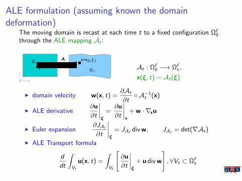
ALE formulation (assuming known the domaindeformation)

The moving domain is recast at each time t to a fixed configuration Ωf0

through the ALE mapping At :

t

0 x=x(t, ξ )

Ω

At

Ωξ At : Ωf

0 −→ Ωft ,

x(ξ, t) = At(ξ)

I domain velocity w(x, t) =∂At

∂t A−1

t (x)

I ALE derivative∂u

∂t

∣∣∣∣ξ

=∂u

∂t

∣∣∣∣x

+ w · ∇xu

I Euler expansion∂JAt

∂t

∣∣∣∣ξ

= JAt div w, JAt = det(∇At)

I ALE Transport formula

d

dt

∫Vt

u(x, t) =

∫Vt

[∂u

∂t

∣∣∣∣ξ

+ u div w

],∀Vt ⊂ Ωf

t

Navier Stokes equations in ALE form

%f∂u

∂t

∣∣∣∣ξ

+ %f ((u−w) · ∇)u− divσf(u, p) = f

div u = 0

in Ωt

Hybrid formulation: the spatial derivative terms are computed on thedeformed configuration Ωf

t , whereas the time derivative is computed onthe reference configuration Ωf

0.

Using the Euler formula, the momentum equation can be equivalentlywritten in conservative form

%fJAt

∂JAt u

∂t

∣∣∣∣ξ

+ %f div((u−w)⊗ u)− divσf(u, p) = f

NS-ALE weak formulation

Consider a test function v ∈ [H10 (Ωf

0)]d defined on the referenceconfiguration, and let us “map” it onto the deformed configuration:v = v (At)

−1.

We multiply the momentum eq. by v and integrate by parts

Non conservative formulation

∫Ωf

t

%f

(∂u

∂t

∣∣∣∣ξ

+ (u−w) · ∇u

)· v + σf :∇v + div uq =

∫Ωf

t

f · v

Again, we can write an alternative conservative formulation by using theALE transport formula

Conservative formulation

d

dt

∫Ωf

t

%f u · v +

∫Ωf

t

%f div((u−w)⊗ u) · v + σf :∇v + div uq =

∫Ωf

t

f · v

Finite Element ALE formulation

We introduce a triangulation Th,0 of the reference domain Ωf0 and choose

finite element spaces (Vh,0,Qh,0) on Th,0 for velocity and pressure resp.

f

wΓ t,hhTs

A t

t,hTT h,0f f

At time t, let Th,t be the image of Th,0 through the mapping At .

Similarly, we define finite element spaces (Vh,t ,Qh,t) on Th,t as the mapof (Vh,0,Qh,0) through At .

Remark. Assume At is a piecewise linear function on Th,0. Then, Th,t isa triangulation of Ωf

t .

Moreover, if Vh,0 (resp Qh,0) is the space of piecewise polynomials ofdegree p on Th,0, then Vh,t (resp Qh,t) is the space of piecewisepolynomials of degree p on Th,t

Finite Element ALE formulation – conservativefind (uh, ph) ∈ (Vh,t ,Qh,t), for each t > 0, such that

d

dt

∫Ωf

t

%f uh · vh+

∫Ωf

t

%f div((uh−wh)⊗uh)·vh+σf :∇vh+div uhqh =

∫Ωf

t

f ·vh

for all (vh, qh) ∈ (Vh,t ,Qh,t)

Algebraic formulation of the momentum equation

d

dt(M(t)U(t))︸ ︷︷ ︸

ALE time der.

+ A(t)U(t)︸ ︷︷ ︸stiffness

+ Nc(t,U−W)U(t)︸ ︷︷ ︸transport

+BT (t)P(t) = F(t)

with Nc(U)ij =∫

Ωdiv((uh −wh)⊗ φj

)· φi

I The two formulations (conservative and non conservative) areequivalent at the time-continuous level. But they lead to differenttime discretization schemes.

I Observe that all matrices depend on time!

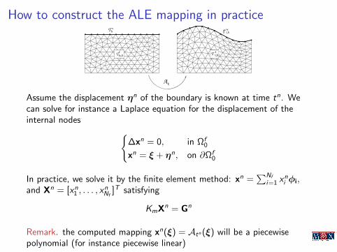
How to construct the ALE mapping in practice

f

wΓt,hhT s

A t

t,hTT h,0f f

Assume the displacement ηn of the boundary is known at time tn. Wecan solve for instance a Laplace equation for the displacement of theinternal nodes

∆xn = 0, in Ωf0

xn = ξ + ηn, on ∂Ωf0

In practice, we solve it by the finite element method: xn =∑Nf

i=1 xni φi,

and Xn = [xn1 , . . . , x

nNf

]T satisfying

KmXn = Gn

Remark. the computed mapping xn(ξ) = Atn(ξ) will be a piecewisepolynomial (for instance piecewise linear)

Some References

[D83] J. Donea, An arbitrary Lagrangian-Eulerian finite element method fortransient fluid-structure interactions Comput. Methods Appl. Mech. Engrg.,33:689–723:1982.

[FGG01] C. Farhat, P. Geuzainne, C. Grandmont, The discrete geometricconservation law and the nonlinear stability of ALE schemes for the solution offlow problems on moving grids, J. Comput. Physics 174:669–694, 2001.

[FN99] L. Formaggia, F. Nobile, A stability analysis for the ArbitraryLagrangian Eulerian formulation with finite elements, East-West J. Num.Math., 7:105–132, 1999.

[FN04] L. Formaggia, F. Nobile, Stability analysis of second-order timeaccurate schemes for ALE-FEM, Comput. Methods Appl. Mech. Engrg.,193:4097–4116, 2004.

[EGP09] S. Etienne, A. Garon, D. Pelletier, Perspective on the geometricconservation law and finite element methods for ALE simulations ofincompressible flow, J. Comput. Physics, 228:2313–2333, 2009.

[JLBL06] J-F. Gerbeau, C. Le Bris, T. Lelievre, Mathematical Methods for theMagnetohydrodynamics of Liquid Metals (Ch. 5), Oxford Univ. Press, 2006

Some References

[HLZ81] T.J.R. Hughes, W.K. Liu, T.K. Zimmermann, Lagrangian-Eulerianfinite element formulation for incompressible viscous flows, Comput. MethodsAppl. Mech. Eng. 29(3):329–349, 1981.

[LF96] M. Lesoinne, C. Farhat, Geometric conservation laws for flow problemswith moving boundaries and deformable meshes, and their impact in aeroelasticcomputations, Comput. Methods Appl. Mech. Engrg. 134:71–90, 1996.

[N00] B. Nkonga, On the conservative and accurate CFD approximations formoving meshes and moving boundaries, Comput. Methods Appl. Mech. Eng.,190:1801–1825, 2000.

[TL79] P.D. Thomas, C.K. Lombard, Geometric conservation law and its

application to flow computations on moving grids, AIAA 17:1030–1037, 1979.

Algorithms for fluid-structure interactionwith large displacements

FSI problem - a three field formulation

Fluid problem F lALE (wn; un, pn) = 0 in Ωfn

Structure problem St(ηn, ηn) = 0; in Ωs0

ALE mapping Mesh(An, An) = 0 in Ωf0

Coupling conditions

kinematic cond. un An = ηn on Γ0

dynamic cond. σf (un, pn)nf = −σs(ηn)ns on Γt

geometric cond. An = ξ + ηn, An = ηn on Γ0

wn = An (An)−1, Ωtn = An(Ωf

0)

Fully coupled non-linear problem in the unknowns (un, pn,An, An,ηn, ηn)

Partitioned versus Monolithic solvers

I We refer to Monolithic schemes when we try to solve thenon-linear problem all at once. We assemble and solve a “huge”linear system in the unknowns un, pn,An, An,ηn, ηn.

I We refer to Partitioned strategies when we solve iteratively thefluid and structure subproblems (never form the full matrix). Thisallows one to couple two existing codes, one solving the fluidequations and the other the structure problem.

I There are other options in between: for instance one can “formally”write the monolithic problem and then use a block preconditioner tosolve it. In this way one recovers partitioned procedures (see e.g.[Heil, CMAME ’04])

Partitioned fluid-structure algorithms

A simple loosely coupled partitioned FSI algorithmGiven the solution (un−1, pn−1,An−1, An−1,ηn−1, ηn−1) at timestep tn−1:

1. Extrapolate the displacement and velocity of the interface: e.g.

˜ηn = ηn−1, ηn = ηn−1 + ∆t ˜ηn, on Γ0

2. Compute the ALE mapping:

Mesh(An, An) = 0 in Ωf

0

An = ξ + ηn, An = ˜ηn on Γ0

3. Solve the fluid problem with Dirichlet boundary conditionsF lALE (wn; un, pn) = 0, in Ωf

n = An(Ωf0)

un = ˜ηn (An)−1, on Γn = An(Γ0)

4. Solve the structure equation with Neumann boundary conditionsSt(ηn, ηn) = 0, in Ωs

0

σs(ηn)ns = −σf (un, pn)nf , on Γn

5. Go to next time step

The staggered algorithm by Farhat and Lesoinne (’98)

A popular algorithm proposed by C. Farhat and M. Lesoinne, CMAME1998, uses staggered grids:

I The fluid equation is discretized with a second order backwarddifference scheme (BDF2) and colocated at tn+1/2

I The ALE mapping is piecewise linear in [tn−1/2, tn+1/2]

I The structure equation is discretized by the mid-point scheme andcollocated at tn+1.

n−1.η

n.ηη

n n+1.ηη

n+1

un−1/2

pn−1/2

un+1/2

pn+1/2

σn+1/2

fηn−1/2

ηn−1

Given the solution (un−1/2, pn−1/2,An−1/2,ηn, ηn):

1. Extrapolate the interface displacement and velocity at tn+1/2:

ηn+1/2 = ηn +∆t

2ηn, ηn+1/2 = ηn, on Γ0

2. Compute the ALE mapping at tn+1/2:

Mesh(An+1/2) = 0

An+1/2 = ξ + ηn+1/2

and A(t) = An+1/2 t − tn−1/2

∆t+An−1/2 tn+1/2 − t

∆t, t ∈ [tn−1/2, tn+1/2]

3. Solve the fluid problem with BDF2 at tn+1/2F lGCLALE (w; un+1/2, pn+1/2) = 0, in Ωf

n+1/2 = An+1/2(Ωf0)

un+1/2 = ηn+1/2 (An+1/2)−1, on Γn = An(Γ0)

4. Solve the structure equation with Mid-Point at tn+1St(ηn+1, ηn+1) = 0, in Ωs

0

σs(ηn+ηn+1

2 )ns = −σf (un+1/2, pn+1/2)nf , on Γn+1/2

5. Go to next time step

On partitioned proceduresPartitioned procedures may have serious stability problems in certainapplications.

Dangerous situations appear for incompressible fluids when the mass ofthe structure is small compared to the mass of the fluid

The instability is due to a non perfect balance of energy transfer at theinterface. For instance, in the algorithm by Farhat & Lesoinne, we have:

Work done in [tn, tn+1] by

fluid Wn+ 1

2

f =

∫Γn+ 1

2

(σf (un+ 12 , pn+ 1

2 )nf ) ·∆tun+ 12

structure Wn+ 1

2s =

∫Γn+ 1

2

(σs(ηn+1 + ηn

2)ns) ·∆t

ηn+1 + ηn

2

Ideally, one would like to have Wn+ 1

2

f + Wn+ 1

2s = 0.

Energy unbalancing: ∆W = Wn+ 1

2

f + Wn+ 1

2s

∆W = −∆t2

∫Γn+1/2

(σf (un+ 12 , pn+ 1

2 )nf ) · ηn+1 − ηn

2∆t= O(∆t2)

A fully implicit partitioned FSI algorithm

To have a perfect energy balance, we need to satisfy exactly at each timestep the kinematic and dynamic coupling conditions.

A possible remedy: fixed point approach: subiterate at each time step,eventually adding a relaxation step

I if ‖ηn − ηn‖ > tol

set ηn ← ωηn + (1− ω)ηn

repeat points 2-4 until convergence

I The fixed point algorithm is stable, in general.

I However, whenever the partitioned procedure is unstable, the fixedpoint may need a very small relaxation parameter ω and theconvergence may be very slow.

A fully implicit partitioned FSI algorithm - Dir. NeumannGiven the solution (un−1, pn−1,An−1,ηn−1, ηn−1) at time step tn−1, setηn

0 = ηn−1 and ηn0 = ηn−1 + ∆tηn and for k = 1, 2, . . .

1. Compute the ALE mapping:Mesh(An

k , Ank) = 0

Ank = ξ + ηn

k−1, Ank = ηn

k−1, on Γ0

2. Solve the fluid problem with Dirichlet boundary conditionsF lALE (wn

k ; unk , p

nk ) = 0, in Ωf

n,k = Ank(Ωf

0)

unk = ηn

k−1 (Ank)−1, on Γn,k = An

k(Γ0)

3. Solve the structure equation with Neumann boundary conditionsSt(ηn

k , ˜ηnk) = 0, in Ωs

0

σs(ηnk)ns = −σf (un

k , pnk )nn, on Γn,k

4. Relaxation step: If ‖ηnk − ηn

k−1‖ > tol , set ηnk = ωηn

k + (1− ω)ηnk−1

(and similarly for ηnk) and go to step 1.

Load transfer between fluid and structureAt the discrete level, there is a proper way of exchanging information.

Conforming finite element spaces at the interface: let φbi

Nb

i=1 be thebasis functions (fluid and structure) corresponding to the interface nodes;

uh|Γ =

Nb∑i=1

uiφbi |Γ, ηh|Γ =

Nb∑i=1

ηiφbi |Γ

and Ub = [u1, . . . , uNb], db = [η1, . . . , ηNb

] are the vectors of dofs.I Fluid Dirichlet b.c. uh = ηh

=⇒ nodal values ui = ηi =⇒ Ub = db

I Structure Neumann b.c. σs · ns = −σf · nf

Fs,i =

∫Γn

−σf (uh, ph)nf ·φbi = < Res(uh, ph),φb

i >︸ ︷︷ ︸−Ff ,i

=⇒ Fbs = −Fb

f

NS

Γ

i

LOAD

Non-conforming finite element spaces at the interface

I φbi

Nbf

i=1: basis functions (fluid) corresponding to the interface

nodes. uh|Γ =∑Nbf

i=1 uiφbi |Γ

I ψbj

Nbs

j=1 basis functions (structure) corresponding to the interface

nodes. ηh|Γ =∑Nbs

j=1 ηjψbj |Γ

Fluid Dirichlet b.cs: unh = Πhη

nh where Πh is a suitable operator (can be

interpolation, L2 projection, etc.). Let Cij such that Πhψbj =

∑Nbf

i=1 Cijφbi |Γ

=⇒ ui =

Nbs∑j=1

Cij ηj =⇒ Ub = C db

Structure Neumann b.cs.: σsns = −Π∗h(σf nf ) (with Π∗h adjoint of Πh)

Fs,j = −∫

Γ

(σf ·nf )·Πhψbj =

Nbs∑i=1

Cij < Res(uh, ph),φbi >︸ ︷︷ ︸

−Ff ,i

, =⇒ Fbs = −CTFb

f

Some references on FSI algorithms

S. Deparis, M. Discacciati, G. Fourestey, A. Quarteroni. Fluid-structurealgorithm based on Steklov-Poincare operators. Comput. Methods Appl.Mech. Engrg., 195, 5797-5812, 2006.

C. Farhat, M. Lesoinne, P. Le Tallec. Load and motion transfer algorithms forfluid/structure interaction problems with non-matching discrete interfaces:momentum and energy conservation, optimal discretization and application toaeroelasticity. Comput. Methods Appl. Mech. Engrg. 157(1-2):95–114, 1998.

C. Farhat, M. Lesoinne. Two efficient staggered algorithms for the serial andparallel solution of three-dimensional nonlinear transient aeroelastic problems.Comput. Methods Appl. Mech. Engrg. 182:499–515, 2000.

U. Kutter, W.A. Wall. Fixed-point fluid-structure interaction solvers withdynamic relaxation, Comput. Mech. 43:61–72, 2009.

P. Le Tallec and J. Mouro. Fluid structure interaction with large structuraldisplacements. Comput. Methods Appl. Mech. Engrg., 190:3039–3067, 2001.

S. Piperno, C. Farhat. Partitioned procedures for the transient solution ofcoupled aeroelastic problems – Part II: energy transfer analysis andthree-dimensional applications. Comput. Methods Appl. Mech. Engrg.124(1-2):79–112, 1995.

Some references on FSI algorithms

S. Badia, F. Nobile and C. Vergara, Fluid-structure partitioned proceduresbased on Robin transmission conditions , J. Comput. Physics, 2008, vol.227/14, pp. 7027-7051

S. Badia, A. Quaini, and A. Quarteroni. Modular vs. non-modularpreconditioners for fluid-structure systems with large added-mass effect.Comput. Methods Appl. Mech. Engrg., in press, 2008.

P. Causin, J.F. Gerbeau, and F. Nobile. Added-mass effect in the design ofpartitioned algorithms for fluid-structure problems. Comput. Methods Appl.Mech. Engrg., 194(42-44):4506–4527, 2005.

M.A. Fernandez and M. Moubachir. A Newton method using exact Jacobiansfor solving fluid-structure coupling. Computers & Structures, 83(2-3):127–142,2005.

M. Heil. An efficient solver for the fully coupled solution of large-displacementfluid-structure interaction problems. Comput. Methods Appl. Mech. Engrg.193(1-2):1–23, 2004.

H.G. Matthies, J. Steindorf. Partioned but strongly coupled iteration schemesfor non-linear fluid-structure interaction, Computers and Structures, 80 (2002),1991-1999.

Acknowledgements

I wish to thank Fabio Nobile for the availability of large part of thematerial used for this lectures.