An Introduction to thePhysics and Technologyof e+e- Linear Colliders

Lecture 1: Introduction and Overview

Nick Walker (DESY)Nick Walker

DESY

DESY Summer Student Lecture31st July 2002USPAS Santa Barbara 16th June, 2003

Course Content

1. Introduction and overview

2. Linac part I

3. Linac part II

4. Damping Ring & Bunch Compressor I

5. Damping Ring & Bunch Compressor II

6. Final Focus Systems

7. Beam-Beam Effects

8. Stability Issues in Linear Colliders

9. the SLC experience and the Current LC Designs

Lecture:

This Lecture

• Why LC and not super-LEP?• The Luminosity Problem

– general scaling laws for linear colliders

• A introduction to the linear collider sub-systems:– main accelerator (linac)– sources– damping rings– bunch compression– final focus

during the lecture, we will introduce (revise) some important basic accelerator physics concepts that we will need in the remainder of the course.

Energy Frontier e+e- Colliders

LEP at CERN, CHEcm = 180 GeVPRF = 30 MW

LEP at CERN, CHEcm = 180 GeVPRF = 30 MW

Why a Linear Collider?

B

Synchrotron Radiation froman electron in a magnetic field:

2222

2BEC

ceP

4

/EC

revE

Energy loss per turn of a machine with an average bending radius :

Energy loss must be replaced by RF system

Cost Scaling $$

• Linear Costs: (tunnel, magnets etc)$lin

• RF costs:$RF E E4/

• Optimum at$lin = $RF

Thus optimised cost ($lin+$RF) scales as E2

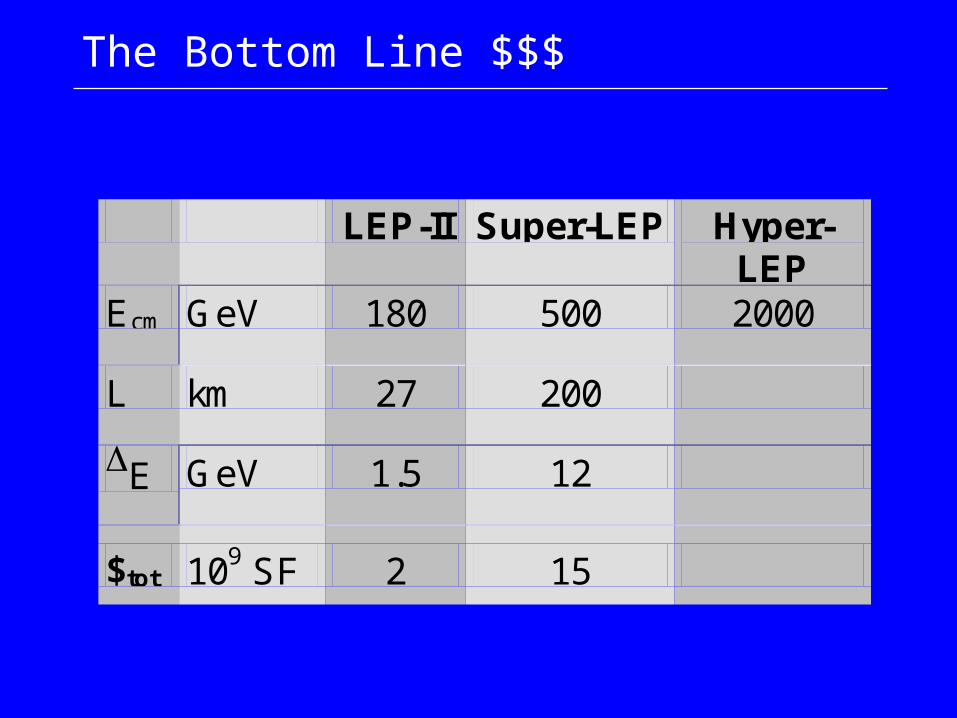
The Bottom Line $$$

LEP-II Super-LEP Hyper-LEP

Ecm GeV 180 500 2000

L km 27

E GeV 1.5

$tot 109 SF 2

The Bottom Line $$$

LEP-II Super-LEP Hyper-LEP

Ecm GeV 180 500 2000

L km 27 200

E GeV 1.5 12

$tot 109 SF 2 15

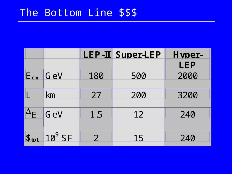
The Bottom Line $$$

LEP-II Super-LEP Hyper-LEP

Ecm GeV 180 500 2000

L km 27 200 3200

E GeV 1.5 12 240

$tot 109 SF 2 15 240

solution: Linear ColliderNo Bends, but lots of RF!

e+ e-

5-10 km

Note: for LC, $tot E

• long linac constructed of many RF accelerating structures

• typical gradients range from 25100 MV/m

A Little History

A Possible Apparatus for Electron-Clashing Experiments (*).

M. Tigner

Laboratory of Nuclear Studies. Cornell University - Ithaca, N.Y.

M. Tigner, Nuovo Cimento 37 (1965) 1228

“While the storage ring concept for providing clashing-beam experiments (1) is very elegant in concept it seems worth-while at the present juncture to investigate other methods which, while less elegant and superficially more complex may prove more tractable.”

A Little History (1988-2003)

• SLC (SLAC, 1988-98)• NLCTA (SLAC, 1997-)• TTF (DESY, 1994-)• ATF (KEK, 1997-)• FFTB (SLAC, 1992-1997)• SBTF (DESY, 1994-1998)• CLIC CTF1,2,3 (CERN, 1994-)

Over 14 Years of Linear Collider

R&D

Past and Future

SLC LC

Ecm 100 500 1000 GeV

Pbeam 0.04 5 20 MW *y 500 (50) 1 5 nm E/Ebs 0.03 3 10 %

L 0.0003 ~3 1034 cm?2s-1

generally quoted as‘proof of principle’

but we have a very long way to go!

LC Status in 1994

TESLA SBLC JLC-S JLC-C JLC-X NLC VLEPP CLIC

f [GHz] 1.3 3.0 2.8 5.7 11.4 11.4 14.0 30.0

L1033

[cm-2s-1]6 4 4 9 5 7 9 1-5

Pbeam

[MW]16.5 7.3 1.3 4.3 3.2 4.2 2.4 ~1-4

PAC

[MW]164 139 118 209 114 103 57 100

y

[10-8m]100 50 4.8 4.8 4.8 5 7.5 15

y*[nm]

64 28 3 3 3 3.2 4 7.4

1994 Ecm=500 GeV

LC Status 2003

TESLA SBLC JLC-S JLC-C JLC-X/NLC VLEPP CLIC

f [GHz] 1.3 5.7 11.4 30.0

L1033

[cm-2s-1]34 14 20 21

Pbeam

[MW]11.3 5.8 6.9 4.9

PAC

[MW]140 233 195 175

y

[10-8m]3 4 4 1

y*[nm]

5 4 3 1.2

2003 Ecm=500 GeV

The Luminosity Issue

2b rep

D

n N fL H

ACollider luminosity (cm2 s1) is

approximately given by

where:

Nb = bunches / trainN = particles per bunchfrep = repetition frequencyA = beam cross-section at IPHD = beam-beam enhancement factor

For Gaussian beam distribution:

2

4b rep

Dx y

n N fL H

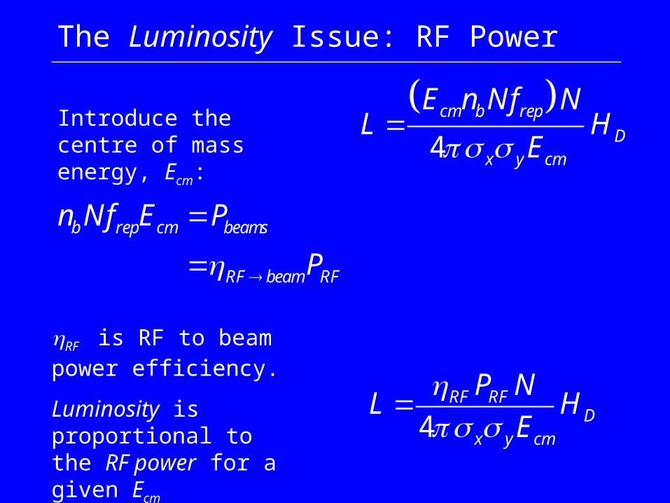
The Luminosity Issue: RF Power

4

cm b rep

Dx y cm

E n Nf NL H

E Introduce the centre of mass

energy, Ecm:

b rep cm beams

RF beam RF

n Nf E P

P

4RF RF

Dx y cm

P NL H

E

RF is RF to beam power efficiency.

Luminosity is proportional to the RF power for a given Ecm

The Luminosity Issue: RF Power

Some numbers:

Ecm = 500 GeVN = 1010

nb = 100frep = 100 Hz

Need to include efficiencies:

RFbeam: range 20-60%Wall plug RF: range 28-40%

AC power > 100 MW just to accelerate beams and achieve luminosity

4RF RF

Dx y cm

P NL H

E

Pbeams = 8 MW

linac technology choice

The Luminosity Issues: storage ring vs LC

4RF RF

Dx y cm

P NL H

E

LEP frep = 44 kHz

LC frep = few-100 Hz (power limited)

factor ~400 in L already lost!

Must push very hard on beam cross-section at collision:

LEP: xy 1306 m2

LC: xy (200-500)(3-5) nm2

factor of 106 gain!Needed to obtain high luminosity of a few 1034 cm-2s-1

The Luminosity Issue: intense beams at IP

1

4 RF RF Dcm x y

NL P H

E

choice of linac technology:• efficiency• available power

Beam-Beam effects:• beamstrahlung• disruption

Strong focusing • optical aberrations• stability issues and

tolerances

The Luminosity Issue: Beam-Beam

• strong mutual focusing of beams (pinch) gives rise to luminosity enhancement HD

• As e± pass through intense field of opposing beam, they radiate hard photons [beamstrahlung] and loose energy

• Interaction of beamstrahlung photons with intense field causes copious e+e pair production [background]

see lecture 2 on beam-beam

6 4 2 0 2 4 63000

2000

1000

0

1000

2000

3000

Ey (

MV

/cm

)

y/y

x y

The Luminosity Issue: Beam-Beam see lecture 2 on beam-beam

,

,

2 e z zx y

beamx y x y

r ND

f

beam-beam characterised by Disruption Parameter:

z = bunch length, fbeam = focal length of beam-lens

3, ,1/ 4

, , ,3,

0.81 ln 1 2ln

1x y x y

Dx y x y x yx y z

DH D D

D

Enhancement factor (typically HD ~ 2):

‘hour glass’ effect

for storage rings, and zbeamf , 1x yD

In a LC, hence zbeamf 10 20yD

The Luminosity Issue: Hour-Glass

= “depth of focus”

reasonable lower limit for is bunch length z

see lecture 2 on beam-beam

2 1 0 1 2Z

3

2

1

0

1

2

3

Y

2 1 0 1 2Z

3

2

1

0

1

2

3

Y

The Luminosity Issue: Beamstrahlung see lecture 2 on beam-beam

3 2

2 20

0.862 ( )

e cmBS

z x y

er E N

m c

RMS relative energy loss

we would like to make xy small to maximise luminosity

BUT keep (x+y) large to reduce SB.

Trick: use “flat beams” with x y 2

2cm

BSz x

E N

Now we set x to fix SB, and make y as small as possible to achieve high luminosity.

For most LC designs, SB ~ 3-10%

The Luminosity Issue: Beamstrahlung

1RF RF

cm x y

P NL

E

Returning to our L scaling law, and ignoring HD

z BS

x cm

N

E

From flat-beam beamstrahlung

3/ 2BS zRF RF

cm y

PL

E

hence

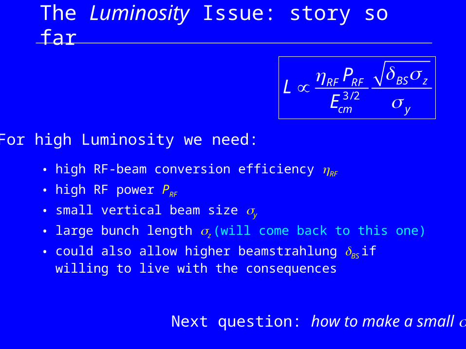
The Luminosity Issue: story so far

• high RF-beam conversion efficiency RF

• high RF power PRF

• small vertical beam size y

• large bunch length z (will come back to this one)

• could also allow higher beamstrahlung BS if willing to live with the consequences

3/ 2BS zRF RF

cm y

PL

E

For high Luminosity we need:

Next question: how to make a small y

The Luminosity Issue: A final scaling law?

3/ 2BS zRF RF

cm y

PL

E

,y n yy

3/ 2, ,

BS BSRF RF z RF RF z

cm n y y cm n y y

P PL

E E

where n,y is the normalised vertical emittance, and y is the vertical -function at the IP. Substituting:

hour glass constraint

y is the same ‘depth of focus’ for hour-glass effect. Hence zy

The Luminosity Issue: A final scaling law?

,

BSRF RFD

cm n y

PL H

E

zy

• high RF-beam conversion efficiency RF

• high RF power PRF

• small normalised vertical emittance n,y

• strong focusing at IP (small y and hence small z)

• could also allow higher beamstrahlung BS if willing to live with the consequences

Above result is for the low beamstrahlung regime where BS ~ few %

Slightly different result for high beamstrahlung regime

Luminosity as a function of y

200 400 600 800 1000

11034

21034

31034

41034

51034

300z m

100z m

500 m

700 m

900 m

( )y m

2 1( )L cm s

2

4b

x y

n N fL

1BS z

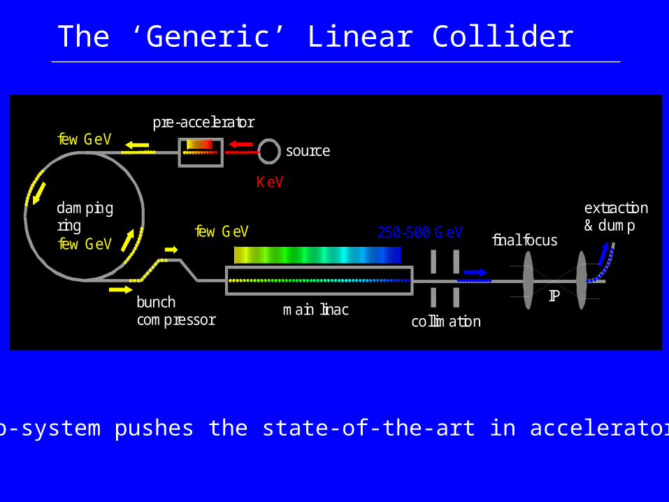
The ‘Generic’ Linear Collider

main linacbunchcompressor

dampingring

source

pre-accelerator

collimation

final focus

IP

extraction& dump

KeV

few GeV

few GeVfew GeV

250-500 GeV

Each sub-system pushes the state-of-the-art in accelerator design

Ez

z

The Linear Accelerator (LINAC) see lectures 3-4 on linac

Ez

z

travelling wave structure:need phase velocity = c(disk-loaded structure)

bunch sees constant field:Ez=E0 cos()

c

c2

ct

standing wave cavity:

bunch sees field:Ez =E0 sin(t+)sin(kz)

=E0 sin(kz+)sin(kz)

c

The Linear Accelerator (LINAC) see lectures 3-4 on linac

Travelling wave structure

Circular waveguide mode TM01 has vp>c

No good for acceleration!

Need to slow wave down using irises.

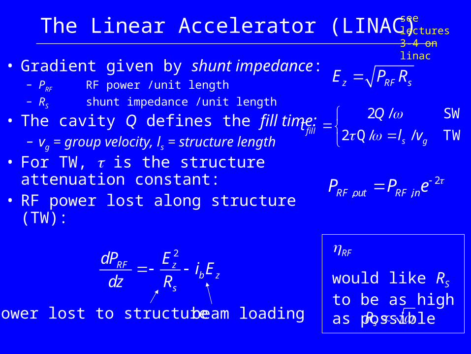
The Linear Accelerator (LINAC)

• Gradient given by shunt impedance:– PRF RF power /unit length– RS shunt impedance /unit length

• The cavity Q defines the fill time:– vg = group velocity, ls = structure length

• For TW, is the structureattenuation constant:

• RF power lost along structure (TW):

see lectures 3-4 on linac

z RF sE P R

2 / SW

2 Q/ / TWfills g

Qt

l v

2, ,RF out RF inP P e

2RF z

b zs

dP Ei E

dz R

power lost to structure beam loading

RF

would like RS to be as high as possible

sR

The Linear Accelerator (LINAC)

• Steady state gradient drops over length of structure due to beam loading

see lectures 3-4 on linac

unloaded

av. loaded

0

0

20

, , 2

2 112 1

z u sz l b

eE E i r

e

assumes constant (stead state) current

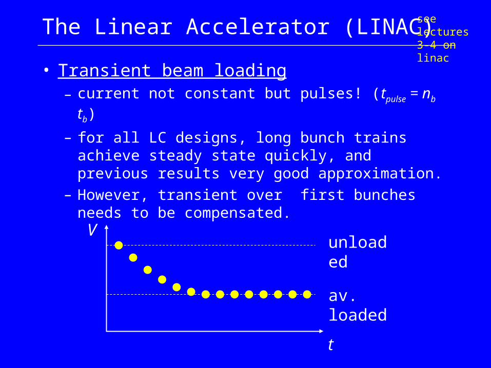
The Linear Accelerator (LINAC)

• Transient beam loading– current not constant but pulses! (tpulse = nb tb)

– for all LC designs, long bunch trains achieve steady state quickly, and previous results very good approximation.

– However, transient over first bunches needs to be compensated.

see lectures 3-4 on linac

unloaded

av. loaded

t

V

The Linear Accelerator (LINAC)

Single bunch beam loading: the Longitudinal wakefield

700 kV/mz bunchE NLC X-band structure:

The Linear Accelerator (LINAC)

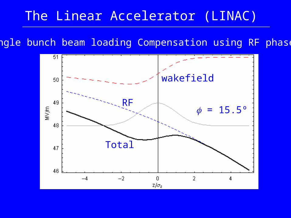
Single bunch beam loading Compensation using RF phase

wakefield

RF

Total

= 15.5º

The Linear Accelerator (LINAC)

Single bunch beam loading: compensation

RMS E/E

Ez

min = 15.5º

Transverse Wakes: The Emittance Killer!

tb

( , ) ( , ) ( , )V t I t Z t

Bunch current also generates transverse deflecting modes when bunches are not on cavity axis

Fields build up resonantly: latter bunches are kicked transversely

multi- and single-bunch beam breakup (MBBU, SBBU)

Damped & Detuned Structures

NLC RDDS1 bunch spacing

Slight random detuning between cells causes HOMs to decohere.

Will recohere later: needs to be damped (HOM dampers)

HOM2Qt

Single bunch wakefields

Effect of coherent betatron oscillation

- head resonantly drives the tail

head

tail

22 0h

y

d yk y

ds

22t

t wf h

d yk y k y

ds

head eom:

tail eom:

Wakefields (alignment tolerances)

bunch

0 km 5 km 10 km

head

head

headtailtail

tail

accelerator axis

cavities

y

tail performsoscillation

RMS

3

1 Z

z

EYNW

f EN

higher frequency = stronger wakefields

-higher gradients

-stronger focusing (smaller )

-smaller bunch charge

The LINAC is only one part

• Produce the electron charge?

• Produce the positron charge?

• Make small emittance beams?

• Focus the beams down to ~nm at the

IP?

Need to understand how to:

main linacbunchcompressor

dampingring

source

pre-accelerator

collimation

final focus

IP

extraction& dump

KeV

few GeV

few GeVfew GeV

250-500 GeV

e+e Sources

• produce long bunch trains of high charge bunches

• with small emittances• and spin polarisation

(needed for physics)

Requirements:

100-1000s @ 5-100 Hzfew nC

nx,y ~ 106,108 m

mandatory for e,nice for e+

Remember L scaling:2

bn

n NL

e Source

• laser-driven photo injector

• circ. polarised photons on GaAs cathode long. polarised e

• laser pulse modulated to give required time structure

• very high vacuum requirements for GaAs (<1011 mbar)

• beam quality is dominated by space charge(note v ~ 0.2c)

120 kV

electrons

laser photons

G aAscathode

= 840 nm

20 m m

510n m

factor 10 in x plane

factor ~500 in y plane

e Source: pre-acceleration

KKK

E = 12 M eV E = 76 M eV

SHB

laser

to D R inecto r linac

solenoids

SHB = sub-harmonic buncher. Typical bunch length from gun is ~ns (too long for electron linac with f ~ 1-3 GHz, need tens of ps)

e Source

e

e

Photon conversion to e± pairs in target material

Standard method is e beam on ‘thick’ target (em-shower)

e

e

ee

ie

N

N

N

N

N

N

N

N

N

N

S

S

S

S

S

S

S

S

S

S ~30MeV photons

0.4X target

undulator (~100m)

250GeV e to IP

frome- linac

e+e- pairs

e Source :undulator-based

• SR radiation from undulator generates photons• no need for ‘thick’ target to generate shower• thin target reduces multiple-Coulomb scattering: hence

better emittance (but still much bigger than needed)• less power deposited in target (no need for mult. systems)• Achilles heel: needs initial electron energy > 150 GeV!

~ 30 MeV

0.4X0

102 m

5 kW

Damping Rings

• (storage) ring in which the bunch train is stored for Tstore ~20-200 ms

• emittances are reduced via the interplay of synchrotron radiation and RF acceleration

2 /( ) DTf eq i eq e

final emittanceequilibriumemittance

initial emittance(~0.01m for e+)

damping time

see lecture 5

pp

dipole RF cavity

y’ not changed by photon (or is it?)

p replaced by RF such that pz = p.

since (adiabatic damping again)

y’ = dy/ds = py/pz,

we have a reduction in amplitude:

y’ = p y’

Must take average over all -phases:

2D

E

P

4

22

cC EP

2

3D E

where and hence

LEP: E ~ 90 GeV, P ~ 15000 GeV/s, D ~ 12 ms

Damping Rings: transverse damping see lecture 5

Damping Rings: Anti-Damping

1

E u

ecB

0

E

ecB

u

ua r

ecB

particle now performs -oscillation about new closed orbit 1 increase in emittance

Equilibrium achieved when

see lecture 5

xdQ

dt

20x

xd

dQ

dt

4

2RF b

EP n N

2

3D E

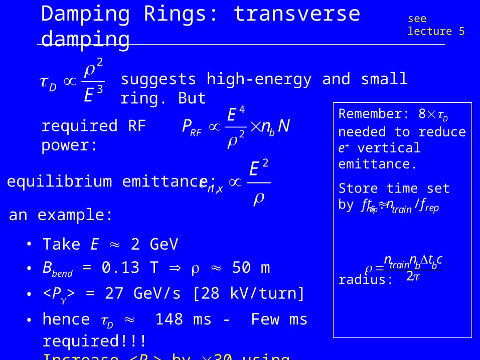
Damping Rings: transverse damping see lecture 5

suggests high-energy and small ring. But

required RF power:

equilibrium emittance:2

,n x

E

• Take E 2 GeV

• Bbend = 0.13 T 50 m

• <P> = 27 GeV/s [28 kV/turn]

• hence D 148 ms - Few ms required!!!Increase <P> by 30 using wiggler magnets

an example:

Remember: 8D needed to reduce e+ vertical emittance.

Store time set by frep:

radius:

/s reptraint n f

2train b b

n n t c

• Horizontal emittance defined by lattice

• theoretical vertical emittance limited by

– space charge

– intra-beam scattering (IBS)

– photon opening angle

• In practice, y limited by magnet alignment errors

[cross plane coupling]

• typical vertical alignment tolerance: y 30 m

requires beam-based alignment techniques!

Damping Rings: limits on vertical emittancesee lecture 5

Bunch Compression

• bunch length from ring ~ few mm• required at IP 100-300 m

RF

z

E /E

z

E /E

z

E /E

z

E /E

z

E /E

long.phasespace

dispersive section

see lecture 6

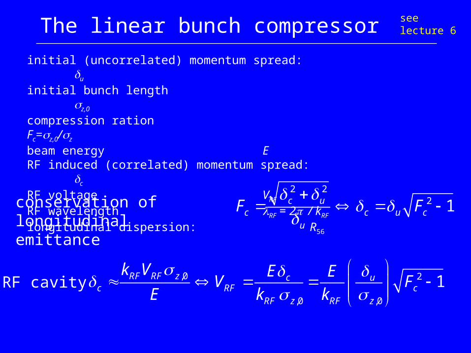
The linear bunch compressor

,0 2

,0 ,0

1RF RF z c uc RF c

RF z RF z

k V E EV F

E k k

2 22 1c u

c c u cu

F F

conservation of longitudinal emittance

RF cavity

initial (uncorrelated) momentum spread: u

initial bunch length z,0

compression ration Fc=z,0/z

beam energy ERF induced (correlated) momentum spread: c

RF voltage VRF

RF wavelength RF = 2/ kRF longitudinal dispersion: R56

see lecture 6

The linear bunch compressor

56z R 2

,0 ,056 2 2 2 2

1c z zRF RF

u u

z k VR

F E F

chicane (dispersive section)

,0

u

1

2mm

0.1%

100 m 20

3 GHz 62.8 m

2 GeV

z

z c

RF RF

F

f k

E

56

2%

318 MV

0.1mRFV

R

see lecture 6

Final Focusing

f1 f2 f2

IP

final doublet

(FD)

Use telescope optics to demagnify beam by factor m = f1/f2= f1/L*

Need typically m = 300

putting L* = 2m f1 = 600m

f1 f2 (=L*)

Final Focusing

*f L

,

* 2 4 m

/

2 5nm 100 300 μm

y n y y

y y

L

remember y ~ z

at final lens y ~ 100 km

short f requires very strong fields (gradient): dB/dr ~ 250 T/mpole tip field B(r = 1cm) ~ 2.5 T

normalised quadrupole strength:

where B = magnetic rigidity = P/e ~ 3.3356 P [GeV/c]

1 0

1 oBK rB

see lecture 7

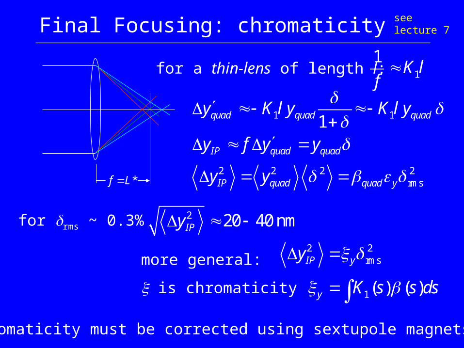
Final Focusing: chromaticity

*f L

for a thin-lens of length l: 1

1K l

f

1 1

2 2 2 2rms

1quad quad quad

IP quad quad

IP quad quad y

y K l y K l y

y f y y

y y

for rms ~ 0.3% 2 20 40 nmIPy 2 2

rms

1( ) ( )

IP y

y

y

K s s ds

more general:

is chromaticity

chromaticity must be corrected using sextupole magnets

see lecture 7

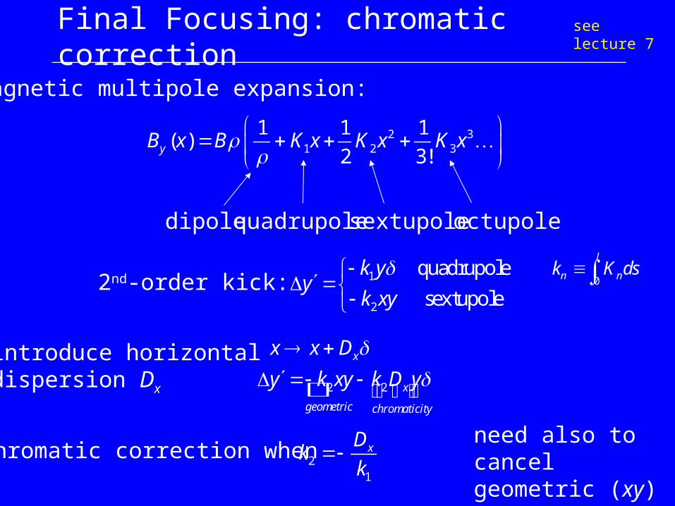
Final Focusing: chromatic correction

magnetic multipole expansion:

2 31 2 3

1 1 1( )

2 3!yB x B K x K x K x

dipole quadrupole sextupole octupole

1

2

quadrupole

sextupole

k yy

k xy

2nd-order kick:

2 2

x

x

geometric chromaticity

x x D

y k xy k D y

0

l

n nk K ds

introduce horizontaldispersion Dx

21

xDk

kchromatic correction when

need also to cancel geometric (xy) term!(second sextupole)

see lecture 7

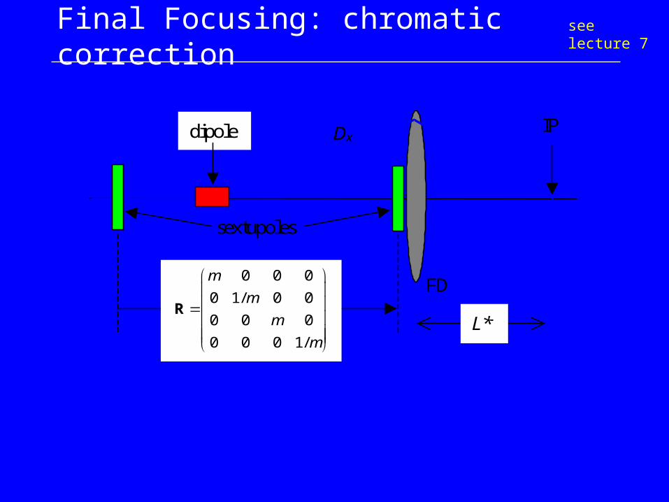
Final Focusing: chromatic correction see lecture 7

IP

FD

Dx

sextupoles

dipole

0 0 0

0 1/ 0 0

0 0 0

0 0 0 1/

m

m

m

m

R

L*

Final Focusing: Fundamental limits

Already mentioned that

At high-energies, additional limits set by so-called Oide Effect:synchrotron radiation in the final focusing quadrupoles leads to a beamsize growth at the IP

zy

1 57 71.83 e e nr F minimum beam size:

occurs when 2 37 72.39 e e nr F

independent of E!

F is a function of the focusing optics: typically F ~ 7(minimum value ~0.1)

see lecture 7

Stability

• Tiny (emittance) beams• Tight component tolerances

– Field quality

– Alignment

• Vibration and Ground Motion issues• Active stabilisation• Feedback systems

Linear Collider will be “Fly By Wire”

see lecture 8

Stability: some numbers

• Cavity alignment (RMS):~ m• Linac magnets: 100 nm• FFS magnets: 10-100 nm• Final “lens”: ~ nm !!!

parallel-to-point focusing:

see lecture 8

0 500 1000 1500 2000

1

0.5

0

0.5

1

0 500 1000 1500 2000

1

0.5

0

0.5

1100nm RMS random offsets

sing1e quad 100nm offset

LINAC quadrupole stability

*,

1 1

**

sin( )

Q QN N

Q i i i Q i ii i

ii i i

y k Y g k Y g

g

* 2

*2 2 2,*

1

sin ( )QN

i Q i i iji

Yy k

for uncorrelated offsets

2 22 2

*2,

0.32

j Q QY

y y n

y N k

take NQ = 400, y ~ 61014 m, ~ 100 m, k1 ~ 0.03 m1 ~25 nm

Dividing by and taking average values:

see lecture 8

*2 * *, /y y n

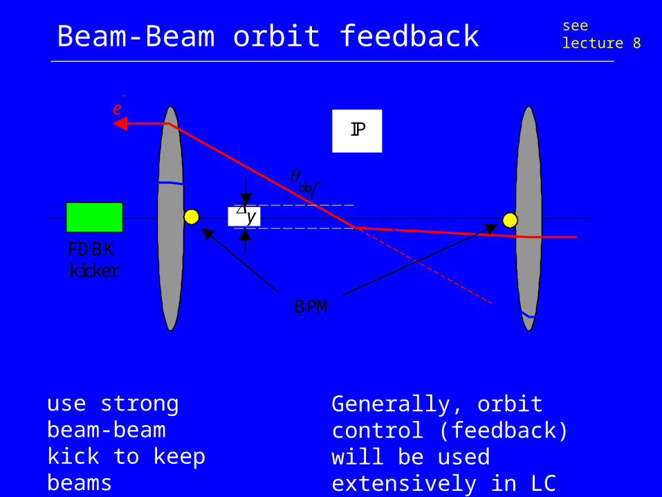
Beam-Beam orbit feedback

use strong beam-beam kick to keep beams colliding

see lecture 8

IP

BPM

bb

FDBK kicker

y

e

e

Generally, orbit control (feedback) will be used extensively in LC

Beam based feedback: bandwidth

0.0001 0.001 0.01 0.1 1

0.05

0.1

0.5

1

5

10

f / frep

g = 1.0g = 0.5g = 0.1g = 0.01

f/frep

Good rule of thumb: attenuate noise with ffrep/20

Ground motion spectra

Long Term Stability

0

0.1

0.2

0.3

0.4

0.5

0.6

0.7

0.8

0.9

1

0.1 1 10 100 1000 10000 100000 1000000

time /s

rela

tive

lum

ino

sity

1 hour 1 day1 minute 10 days

No Feedback

beam-beam feedback

beam-beam feedback +

upstream orbit control

understanding of ground motion and vibration spectrum important

example of slow diffusive ground motion (ATL law)

see lecture 8

Here Endeth the First Lecture