An Introduction to Pseudopotentials

CECAM GIPAW-NMR Tutorial, 23 Sep. 2009

– Typeset by FoilTEX –

Norm-Conserving Pseudopotentials

Electron-ionic core interactions are typically represented by a nonlocal Norm-Conserving Pseudopotential (NCPP): a soft potential for valence electrons only(core electrons disappear from the calculation) having pseudo-wavefunctionscontaining no “orthonormality wiggles”

In many systems, NCPP’s allow accurate calculations with moderate-size (Ec ∼10− 20Ry) plane-wave basis sets

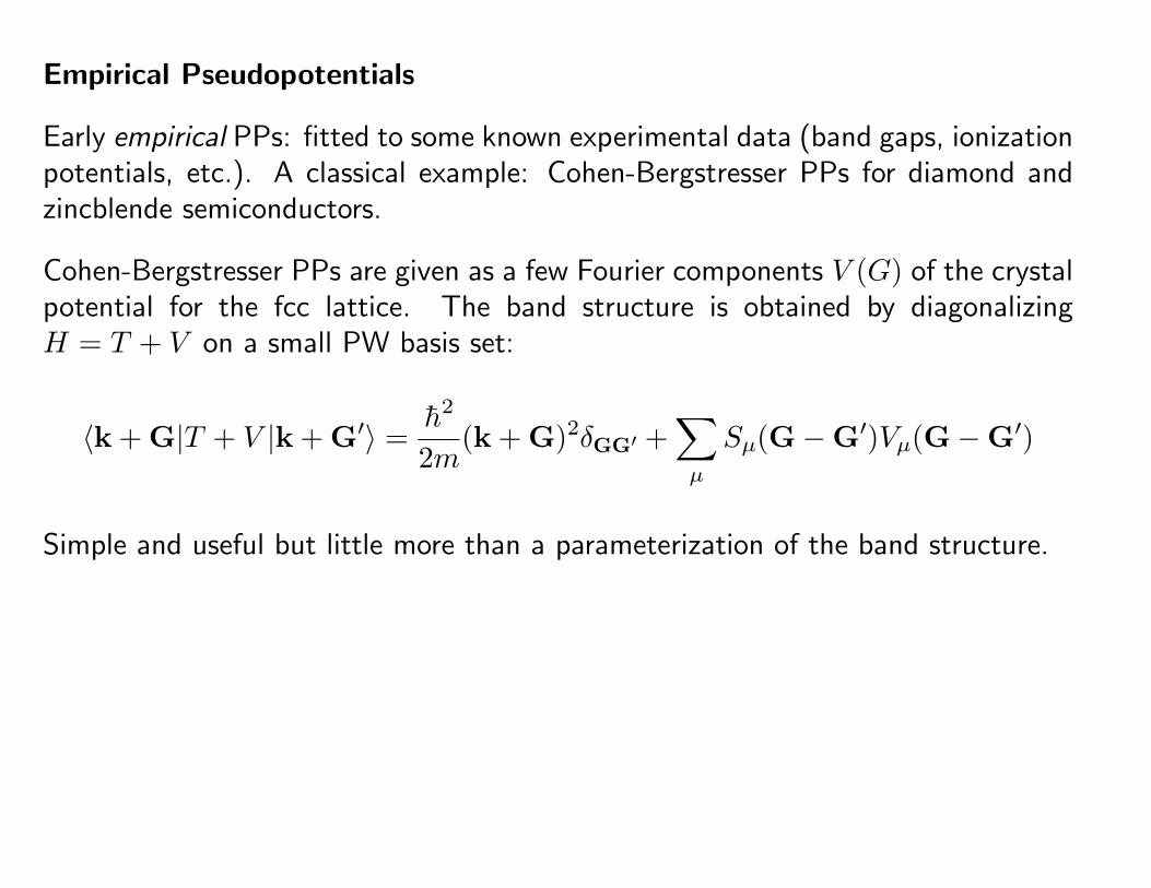
Empirical Pseudopotentials

Early empirical PPs: fitted to some known experimental data (band gaps, ionizationpotentials, etc.). A classical example: Cohen-Bergstresser PPs for diamond andzincblende semiconductors.

Cohen-Bergstresser PPs are given as a few Fourier components V (G) of the crystalpotential for the fcc lattice. The band structure is obtained by diagonalizingH = T + V on a small PW basis set:

〈k + G|T + V |k + G′〉 =h2

2m(k + G)2δGG′ +

∑µ

Sµ(G−G′)Vµ(G−G′)

Simple and useful but little more than a parameterization of the band structure.

Atomic Pseudopotentials

Early atomic , transferrable PPs for self-consistent calculations:

V (r) = −e2∫

n0(r′)|r− r′|

dr′ +(v1 + v2r

2)e−αr2

Appelbaum and Hamann (1973) Silicon, where:

n0(r) = Zv

(απ

)32e−αr2

is assumed to be the ionic electron (pseudo) charge-density distribution (Zv =number of valence electrons). May also be written as

V (r) = −Zve2erf(

√αr)r

+(v1 + v2r

2)e−αr2

Able to reproduce the band structure of crystalline Si, but also useful in othercalculations. Still lacking a first-principle derivation.

Fourier transform for Appelbaum-Hamann PP:

V (G) =1Ω

∫e−iG·rV (r)dr = −4πZve

2

ΩG2e−

G2

4α +1Ω

(πα

)32

[v1 +

v2α

(32− G2

4α

)]e−

G2

4α

The G = 0 term is divergent, but its divergence is compensated by the divergencein the Hartree term:

〈k + G|VH|k + G′〉 =1NΩ

∫e−i(G−G′)·rVH(r)dr = 4πe2

n(G)G2

where n(r) is the self-consistent charge,

VH(r) =∫

n(r′)|r− r′|

dr′.

Note that n(G = 0) = (∑Zv)/Ω. Consider the case of one atom per unit cell for

simplicity:

limG→0

(4πZve

2

ΩG2+ V (G)

)=πe2Zv

Ωα+

1Ω

(πα

)32

(v1 +

32v2α

).

Norm-Conserving Pseudopotentials:

Norm-Conserving, DFT-based PPs were introduced by Hamann, Schluter, Chiangin 1979. For a given reference atomic configuration, they must meet the followingconditions:

• εpsl = εae

l

• φpsl (r) is nodeless

• φpsl (r) = φae

l (r) for r > rc

•∫

r<rc

|φpsl (r)|2r2dr =

∫r<rc

|φael (r)|2r2dr

where φael (r) is the radial part of the atomic valence wavefunction with l angular

momentum, εael its orbital energy. The core radius rc is approximately at the

outermost maximum of the wavefunction.

All-electron vs Pseudowavefunctions:

Features of Norm-conserving Pseudopotentials:

+ transferrable: their construction ensures that they reproduce the logarithmicderivatives, i.e., the scattering properties, of the true potential in a wide rangeof energies. See the identity

−2π[(rφ(r))2

d

dε

(d

drlnφ(r)

)]rc

= 4π∫ rc

0

|φ(r)|2r2dr

valid for any regular solution of the Schrodinger equation at energy ε.

– non local: there is one potential per angular momentum:

V ps(r) =∑

l

Vl(r)|l〉〈l|.

Traditionally PPs are split into a local part, long-ranged and behaving like −Zve2/r

for r →∞, and a short-ranged semilocal term:

V ps = Vloc+ VSL, Vloc ≡ Vloc(r), VSL ≡∑lm

Vl(r)δ(r−r′)Ylm(r)Y ∗lm(r′),

All-electron vs Pseudo logarithmic derivatives:

Generation of norm-conserving Pseudopotentials:

1. From an all-electron self-consistent DFT calculation in an atom with a givenreference configuration, calculate φat

l and εatl , by solving the radial Kohn-Sham

equation. In the non relativistic case:

− h2

2md2φl(r)dr2

+

(h2

2ml(l + 1)r2

+ V (r)− εl

)φl(r) = 0 (1)

2. Generate φpsl for valence states that obey norm-conservation conditions, and

invert the Kohn-Sham equation at εpsl to get Vl(r) (or, generate a Vl(r) in such

a way that φpsl and εps

l obey norm-conservation conditions)

3. Unscreen Vl(r) by removing valence contribution to Hartree and exchange-correlation potentials:

V psl (r) = Vl(r)− VH(nps(r))− Vxc(nps(r))

where nps(r) is the atomic valence charge density (assumed to be spherical):

nps(r) =14π

∑l

fl|φpsl (r)|2

(fl is the occupancy of state with angular momentum l).

Desirable characteristics of a Pseudopotential:

• Transferability: can be estimated from atomic calculations on differentconfigurations. In many cases simple unscreening produces an unacceptableloss of transferability. May require the nonlinear core correction:

V psl (r) = Vl(r)− VH(nps(r))− Vxc(nc(r) + nps(r))

where nc(r) is the core charge of the atom (Froyen, Louie, Cohen 1982)

• Softness: atoms with strongly oscillating pseudo-wavefunctions (first-rowelements, elements with 3d and 4f valence electrons) will produce hard PPsrequiring many PWs in calculations. Larger core radius means better softnessbut worse transferability. Various recipes to get optimal smoothness withoutcompromising transferability: Troullier and Martins (1990), Rappe Rabe KaxirasJoannopoulos (1990)

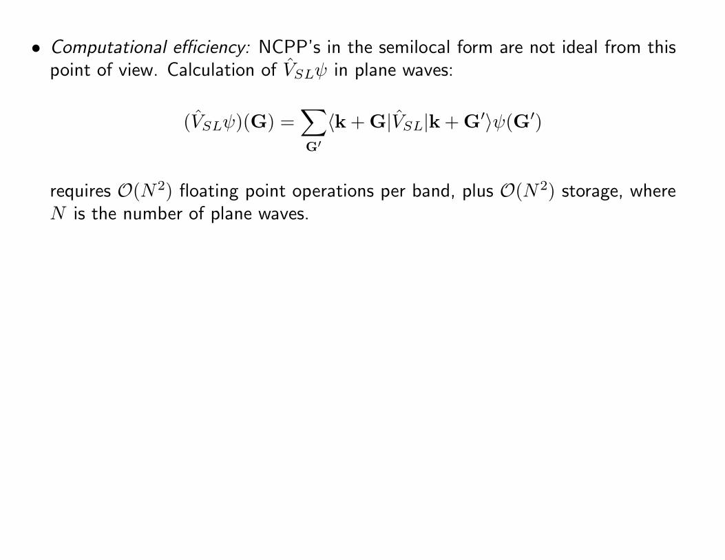
• Computational efficiency: NCPP’s in the semilocal form are not ideal from thispoint of view. Calculation of VSLψ in plane waves:

(VSLψ)(G) =∑G′

〈k + G|VSL|k + G′〉ψ(G′)

requires O(N2) floating point operations per band, plus O(N2) storage, whereN is the number of plane waves.

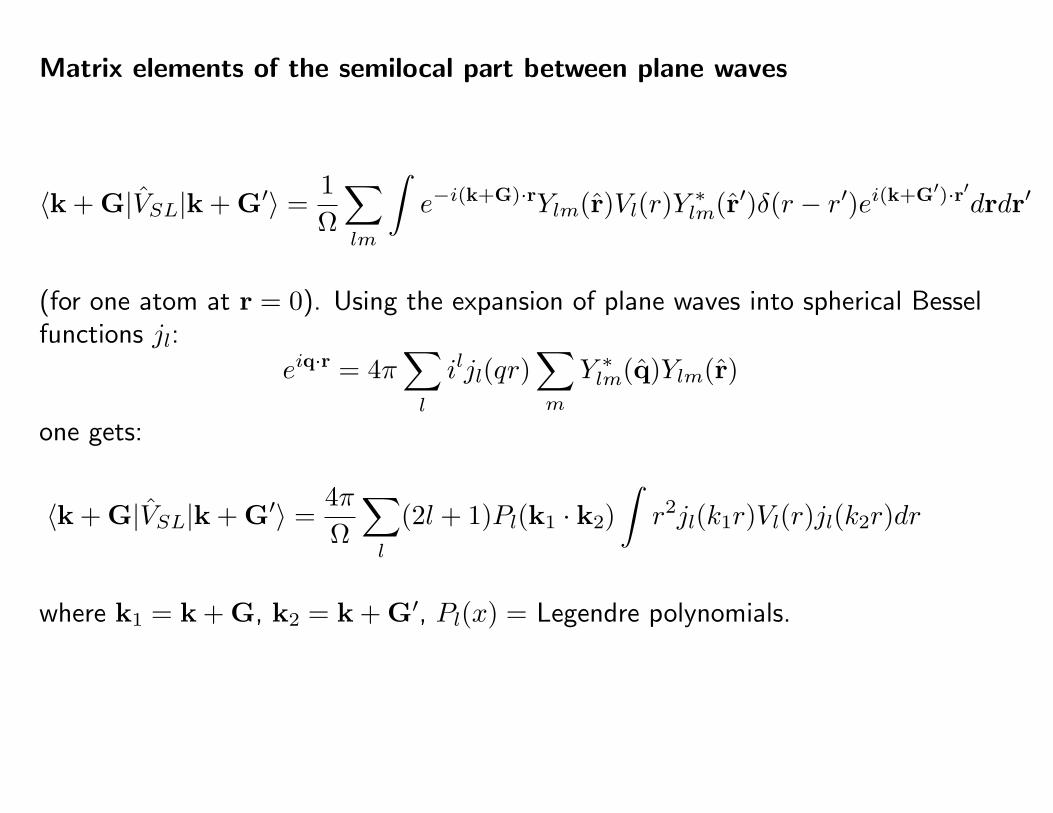
Matrix elements of the semilocal part between plane waves

〈k + G|VSL|k + G′〉 =1Ω

∑lm

∫e−i(k+G)·rYlm(r)Vl(r)Y ∗

lm(r′)δ(r − r′)ei(k+G′)·r′drdr′

(for one atom at r = 0). Using the expansion of plane waves into spherical Besselfunctions jl:

eiq·r = 4π∑

l

iljl(qr)∑m

Y ∗lm(q)Ylm(r)

one gets:

〈k + G|VSL|k + G′〉 =4πΩ

∑l

(2l + 1)Pl(k1 · k2)∫r2jl(k1r)Vl(r)jl(k2r)dr

where k1 = k + G, k2 = k + G′, Pl(x) = Legendre polynomials.

Separable (Kleinman-Bylander) form of pseudopotentials

It is very convenient to recast NCPP’s into a separable, fully nonlocal form:

V ≡ Vloc(r) +∑nm

|βn〉Dnm〈βm|

Introduce the following transformation, proposed by Kleinman and Bylander (KB):

V ps → VKB = V ′loc + VNL

where:

VNL =∑lm

|V ′l φ

pslm〉〈V ′

l φpslm|

〈φpslm|V ′

l |φpslm〉

≡∑lm

vl|βlm〉〈βlm|,

V ′l (r) = Vl(r) − V0(r), V ′

loc ≡ Vloc(r) + V0(r), and V0(r) an arbitrary function.The |φps

lm〉 are the atomic pseudo-wavefunction (including angular term) for thereference state.

The separable form is an approximation if applied to a NCPP generated usingthe Hamann-Schluter-Chiang procedure: on the reference state, VKB|φps

lm〉 =V ps|ψps

lm〉; on states not too far from the reference state, VKB|φlm〉 ' V ps|ψl〉.

Why the separable form?

The separable form usually yields good results, but may badly fail in some casesdue to the appearence of ghosts: states with a wrong number of nodes.

Separable pseudopotentials are computationally much more efficient than theconventional (semilocal) form. The calculation of VNLψ in plane waves:

(VNLψ)(G) =∑G′

〈k + G|VNL|k + G′〉ψ(G′) =p∑

i=1

viβi(G′)∑G′

β∗i (G′)ψ(G′)

requires only O(pN) floating point operations per band and O(pN) storage, wherep is the number of projectors in the system.

〈k + G|VKB|k + G′〉 =1Ω

∑lm

1〈φps

l |V ′l |φ

psl 〉

∫e−i(k+G)·rV ′

l (r)φpsl (r)Ylm(r)dr

×∫ei(k+G′)·r′V ′

l (r′)φpsl (r′)Y ∗

lm(r′)dr′

(for one atom at r = 0).

Using the expansion of plane waves into spherical Bessel functions one gets:

〈k + G|VKB|k + G′〉 =4πΩ

∑lm

1〈φps

l |V ′l |φ

psl 〉Ylm(k1)

∫r2jl(k1r)V ′

l (r)φpsl (r)dr

× Y ∗lm(k2)

∫r2jl(k2r)V ′

l (r)φpsl (r)dr.

where k1 = k + G, k2 = k + G′.

Direct generation of norm-conserving pseudopotentials in separable form

Pseudopotentials can be directly produced in separable form (Vanderbilt 1991).

– generate a local potential Vloc(r) such that Vloc(r) = V (r) for r > rL; Vloc(r)for r < rL can be any smooth regular function

– generate atomic waves |φi〉: regular solutions of the KS equations, not necessarilybound, at a given energy εi. There may be more than one such waves perangular momentum: this increases the transferability.

– generate the corresponding pseudowaves |φi〉, such that φi(r) = φi(r) forr > rc,i

– generate the corresponding functions |χi〉 (vanishing for r > rc,i):

|χi〉 = (εi − T − Vloc)|φi〉;

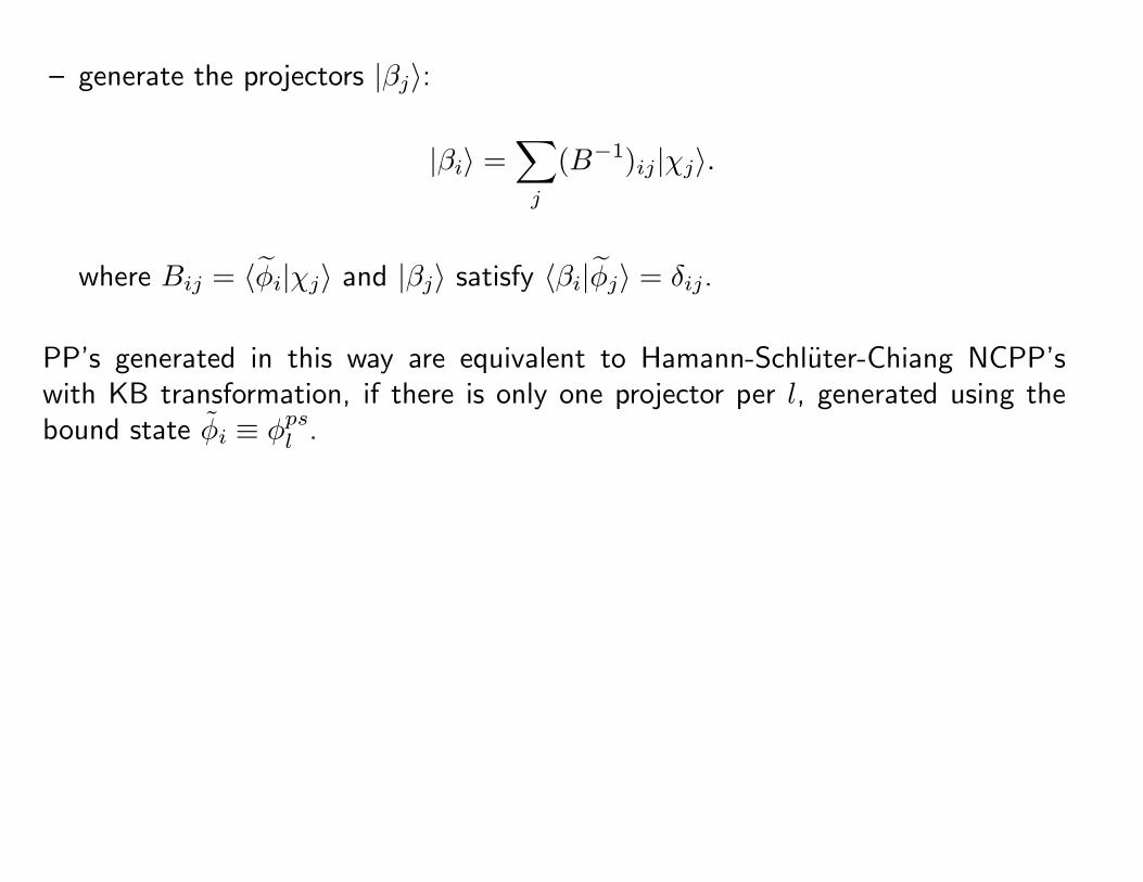
– generate the projectors |βj〉:

|βi〉 =∑

j

(B−1)ij|χj〉.

where Bij = 〈φi|χj〉 and |βj〉 satisfy 〈βi|φj〉 = δij.

PP’s generated in this way are equivalent to Hamann-Schluter-Chiang NCPP’swith KB transformation, if there is only one projector per l, generated using thebound state φi ≡ φps

l .

Limitations of norm-conserving pseudopotentials

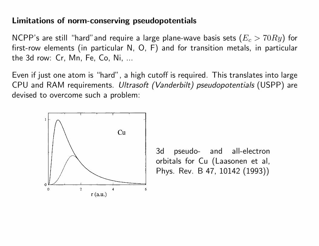
NCPP’s are still “hard”and require a large plane-wave basis sets (Ec > 70Ry) forfirst-row elements (in particular N, O, F) and for transition metals, in particularthe 3d row: Cr, Mn, Fe, Co, Ni, ...

Even if just one atom is “hard”, a high cutoff is required. This translates into largeCPU and RAM requirements. Ultrasoft (Vanderbilt) pseudopotentials (USPP) aredevised to overcome such a problem:

3d pseudo- and all-electronorbitals for Cu (Laasonen et al,Phys. Rev. B 47, 10142 (1993))

Ultrasoft pseudopotentials

VUS ≡ Vloc(r) +∑lm

Dlm|βl〉〈βm|

Charge density with USPP:

n(r) =∑

i

|ψi(r)|2 +∑

i

∑lm

〈ψi|βl〉Qlm(r)〈βm|ψi〉

where the Qlm (“augmentation charges”) are:

Qlm(r) = φ∗l (r)φm(r)− φ∗l (r)φm(r)

|βl〉 are “projectors”|φl〉 are atomic states (not necessarily bound)

|φl〉 are pseudo-waves (coinciding with|φl〉 beyond some “core radius”)

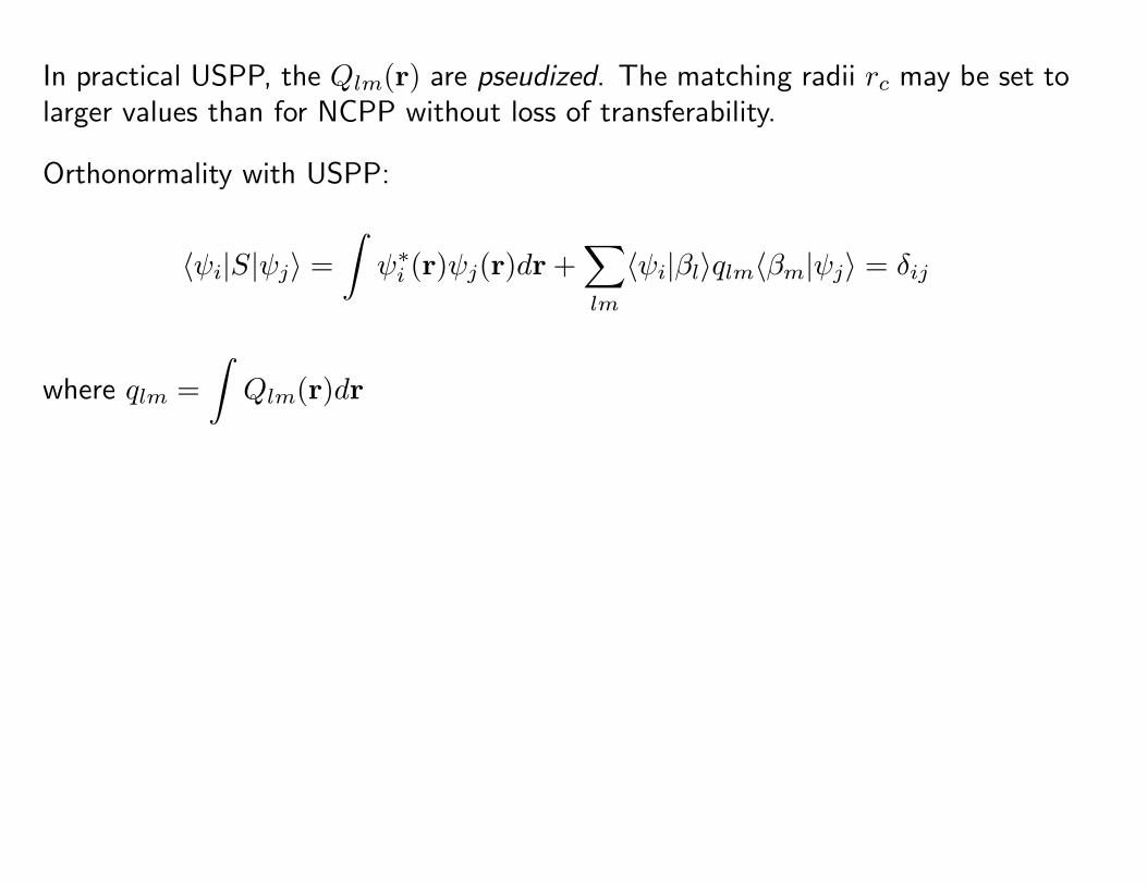
In practical USPP, the Qlm(r) are pseudized. The matching radii rc may be set tolarger values than for NCPP without loss of transferability.

Orthonormality with USPP:

〈ψi|S|ψj〉 =∫ψ∗i (r)ψj(r)dr +

∑lm

〈ψi|βl〉qlm〈βm|ψj〉 = δij

where qlm =∫Qlm(r)dr

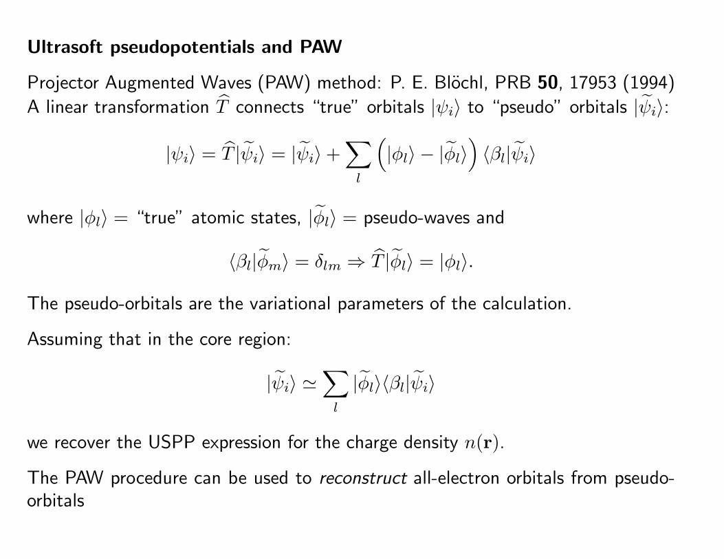
Ultrasoft pseudopotentials and PAW

Projector Augmented Waves (PAW) method: P. E. Blochl, PRB 50, 17953 (1994)

A linear transformation T connects “true” orbitals |ψi〉 to “pseudo” orbitals |ψi〉:

|ψi〉 = T |ψi〉 = |ψi〉+∑

l

(|φl〉 − |φl〉

)〈βl|ψi〉

where |φl〉 = “true” atomic states, |φl〉 = pseudo-waves and

〈βl|φm〉 = δlm ⇒ T |φl〉 = |φl〉.

The pseudo-orbitals are the variational parameters of the calculation.

Assuming that in the core region:

|ψi〉 '∑

l

|φl〉〈βl|ψi〉

we recover the USPP expression for the charge density n(r).

The PAW procedure can be used to reconstruct all-electron orbitals from pseudo-orbitals

Ultrasoft pseudopotential generation:

– generate a local potential Vloc(r) such that Vloc(r) = V (r) for r > rL

– generate the pseudowaves |φi〉 such that φi(r) = φi(r) for r > rc,i

– generate a set of functions |χi〉 (vanishing for r > rc,i):

|χi〉 = (εi − T − Vloc)|φi〉

– generate the projectors |βj〉:

|βi〉 =∑

j

(B−1)ij|χj〉.

where Bij = 〈φi|χj〉 and |βj〉 satisfy 〈βi|φj〉 = δij

– define (pseudized) augmentation functions Qjk:

Qjk(r) = φ∗j(r)φk(r)− φ∗j(r)φk(r)

– define Dij = Bij + εjQij, where

Qij =∫

r<rc,i

(φ∗i (r)φj(r)− φ∗i (r)φj(r)

)dr

– “unscreen” Dij and Vloc:

D0ij = Dij−

∫Qjk(r)Vloc(r)dr, V ion

loc (r) = Vloc(r)−∫dr′

n(r′)|r− r′|

−Vxc(r),

The pseudo-potential is finally given by

VUS = V ionloc +

∑ij

D(0)ij |βi〉〈βj|,

the charge density by

n(r) =∑

i

|φi(r)|2 +∑jk

Qjk(r)〈φi|βj〉〈βk|φi〉.

Plane-waves + Ultrasoft pseudopotential calculations

• there are additional terms in the charge density and in the forces

• electronic states are orthonormal with an overlap matrix S: 〈ψi|S|ψj〉 = δij

• if the ”augmentation charges” are evaluated in G-space, a different (larger)cutoff for them may be required

Various tricks: ”box grids”, r-space evaluation, allow to minimize the CPU timerequired by additional USPP-specific terms