An introduction to persistent homology Computing the 0-barcodes

MUSTAFA HAJIJ

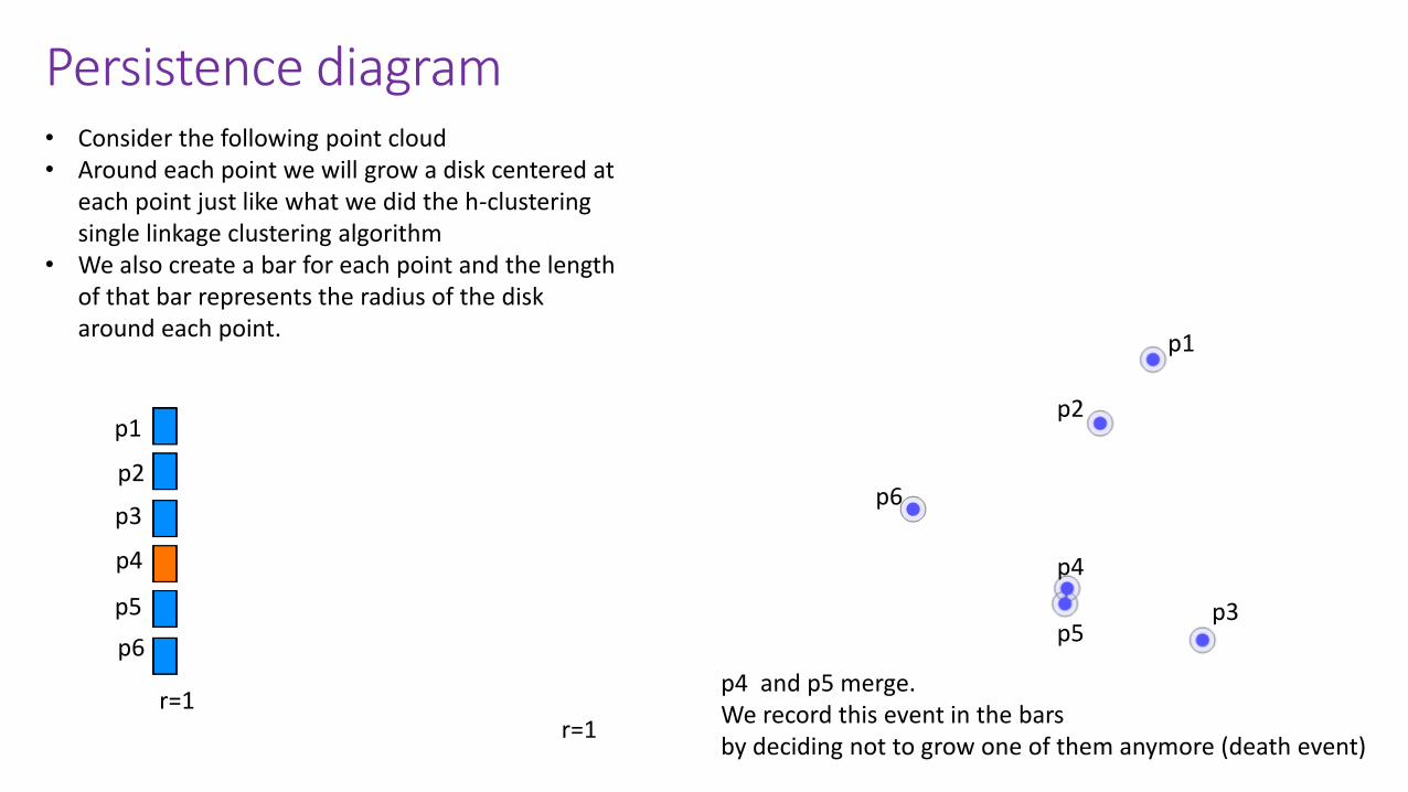
Persistence diagram• Consider the following point cloud• Around each point we will grow a disk centered at

each point just like what we did the h-clustering single linkage clustering algorithm

• We also create a bar for each point and the length of that bar represents the radius of the disk around each point.

p1

p2

p3

p4

p5

p6

p1

p2

p3

p4

p5

p6

r=0r=0

Persistence diagram• Consider the following point cloud• Around each point we will grow a disk centered at

each point just like what we did the h-clustering single linkage clustering algorithm

• We also create a bar for each point and the length of that bar represents the radius of the disk around each point.

p1

p2

p3

p4

p5

p6

p1

p2

p3

p4

p5

p6

r=1

p4 and p5 merge. We record this event in the barsby deciding not to grow one of them anymore (death event)

r=1

Persistence diagram• Consider the following point cloud• Around each point we will grow a disk centered at

each point just like what we did the h-clustering single linkage clustering algorithm

• We also create a bar for each point and the length of that bar represents the radius of the disk around each point.

p1

p2

p3

p4

p5

p6

p1

p2

p3

p4

p5

p6

r=1

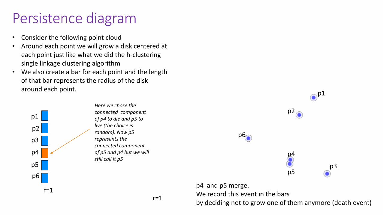
p4 and p5 merge. We record this event in the barsby deciding not to grow one of them anymore (death event)

r=1

Here we chose the connected component of p4 to die and p5 to live (the choice is random). Now p5 represents the connected component of p5 and p4 but we will still call it p5

Persistence diagram• Consider the following point cloud• Around each point we will grow a disk centered at

each point just like what we did the h-clustering single linkage clustering algorithm

• We also create a bar for each point and the length of that bar represents the radius of the disk around each point.

p1

p2

p3

p4

p5

p6

p1

p2

p3

p4

p5

p6

r=3

p1 and p2 merge. We record this event in the barsby deciding not to grow one of them anymore (death event)

r=3

Persistence diagram• Consider the following point cloud• Around each point we will grow a disk centered at

each point just like what we did the h-clustering single linkage clustering algorithm

• We also create a bar for each point and the length of that bar represents the radius of the disk around each point.

p1

p2

p3

p4

p5

p6

p1

p2

p3

p4

p5

p6

r=3

p1 and p2 merge. We record this event in the barsby deciding not to grow one of them anymore (death event)

r=3

Here we chose the connected component of p2 to die and the connected component of p1 to live. Now p1 (the one that lives) represents the connected component of p1 and p2.

Persistence diagram• Consider the following point cloud• Around each point we will grow a disk centered at

each point just like what we did the h-clustering single linkage clustering algorithm

• We also create a bar for each point and the length of that bar represents the radius of the disk around each point.

p1

p2

p3

p4

p5

p6

p1

p2

p3

p4

p5

p6

r=4

The connected component(p5,p4) and the point p3 mergewe record this event in the barsby deciding to stop growing one bar of these connected components

r=4

Persistence diagram• Consider the following point cloud• Around each point we will grow a disk centered at

each point just like what we did the h-clustering single linkage clustering algorithm

• We also create a bar for each point and the length of that bar represents the radius of the disk around each point.

p1

p2

p3

p4

p5

p6

p1

p2

p3

p4

p5

p6

r=5

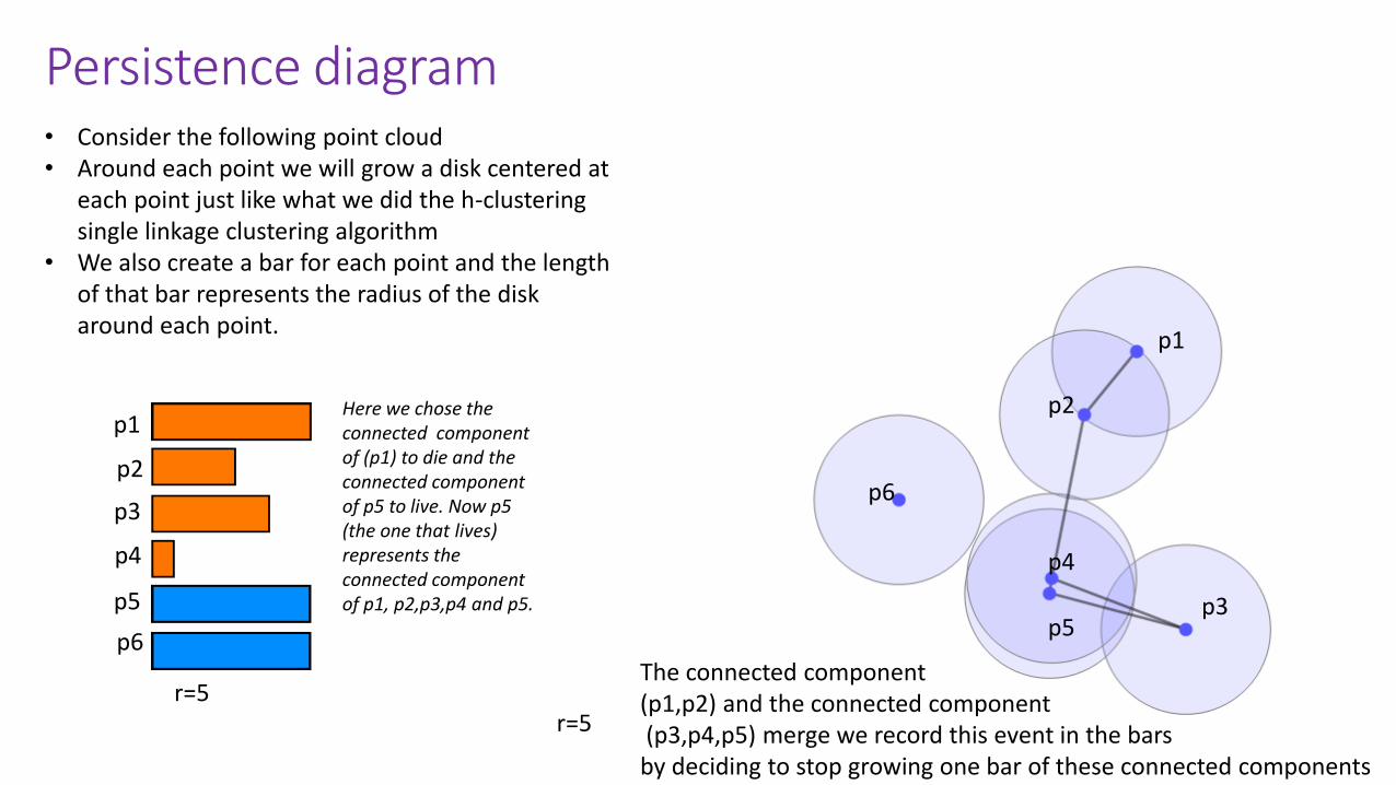
The connected component(p1,p2) and the connected component(p3,p4,p5) merge we record this event in the bars

by deciding to stop growing one bar of these connected components

r=5

Persistence diagram• Consider the following point cloud• Around each point we will grow a disk centered at

each point just like what we did the h-clustering single linkage clustering algorithm

• We also create a bar for each point and the length of that bar represents the radius of the disk around each point.

p1

p2

p3

p4

p5

p6

p1

p2

p3

p4

p5

p6

r=5

The connected component(p1,p2) and the connected component(p3,p4,p5) merge we record this event in the bars

by deciding to stop growing one bar of these connected components

r=5

Here we chose the connected component of (p1) to die and the connected component of p5 to live. Now p5 (the one that lives) represents the connected component of p1, p2,p3,p4 and p5.

Persistence diagram• Consider the following point cloud• Around each point we will grow a disk centered at

each point just like what we did the h-clustering single linkage clustering algorithm

• We also create a bar for each point and the length of that bar represents the radius of the disk around each point.

p1

p2

p3

p4

p5

p6

p1

p2

p3

p4

p5

p6

r=6

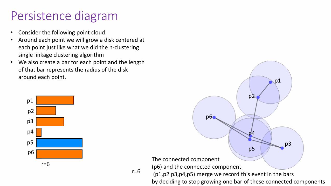
The connected component(p6) and the connected component(p1,p2 p3,p4,p5) merge we record this event in the bars

by deciding to stop growing one bar of these connected components

r=6

Persistence diagram• The resulting diagram barcode is called the 0-barcode. • The 0-barcode is a signature of the point cloud. It encodes topological and geometrical information

of the point cloud in meaningful way.• Long bars represents natural connected components.• Short bars represent points that are close to each other.• If we change the point cloud by a little bit, and recompute the barcodes again then newbarcode is very close to the old one.

p1

p2

p3

p4

p5

p6

p1

p2

p3

p4

p5

p6

Examples• 3 long bars, everything else represent noise

Computed using ripser

Examples• 4 long bars, everything else represent noise

Computed using ripser

Examples• 4 long bars, everything else represent noise

Computed using ripser

Ripserhttp://live.ripser.org/

Barcode when a distance matrix is given

A B C D E F

ABCDE

In this case, the points Coordinate are not given Explicitly. Only the distance between the points are given

The same computation can be carried out

Recall : Kruskal’s Algorithm

Let 𝐺 = (𝑉, 𝐸, 𝑤) be a connected weighted graph.

1. Set 𝑉𝑇 𝑡𝑜 𝑏𝑒 𝑉, 𝑆𝑒𝑡 𝐸𝑇 = {}. Let 𝑆 = 𝐸2. While 𝑆 is not empty and 𝑇 is not a spanning tree

1. Select an edge e from 𝑆 with the minimum weight and delete e from 𝑆.2. If 𝑒 connects two separate trees of 𝑇 then add 𝑒 to 𝐸𝑇

Informally, the algorithm can be given by the following three steps :

Algorithm for computing the 0-barcodeData: A distance matrix M

Result:1-Create the complete graph G associated with the matrix M 2-Initiate an empty UnionFind U.3- for each node vi in G :

1. U.add(vi)2. Create a bar Bi with birth = 0 and death = ∞

4-Sort the edges of G in increasing order5-for each edge ei in G do:

1. If ei connects two different sets C1 and C2 then1. Join C1 and C2 2. Set the death of B1 to w(ei)

The complete graph associated with a distance matrix M : complete graph with e(i,j)=M(i,j).

Algorithm for computing the 0-barcodeData: A distance matrix M

Result:1-Create the complete graph G associated with the matrix M 2-Initiate an empty UnionFind U.3- for each node vi in G :

1. U.add(vi)2. Create a bar Bi with birth = 0 and death = ∞

4-Sort the edges of G in increasing order5-for each edge ei in G do:

1. If ei connects two different sets C1 and C2 then1. Join C1 and C2 2. Set the death of B1 to w(ei)

This is essentially Kruskal’s algorithm

The complete graph associated with a distance matrix M : complete graph with e(i,j)=M(i,j).

Algorithm for computing the 0-barcode with a given max value

Data: A distance matrix M, maximal value ε

Result:1-Create the ε-neighborhood graph of M2-Initiate an empty UnionFind U.3- for each node vi in G :

1. U.add(vi)2. Create a bar Bi with birth = 0 and death = ∞

4-Sort the edges of G in increasing order5-for each edge ei in G do:

1. If ei connects two different sets C1 and C2 then1. Join C1 and C2 2. Set the death of B1 to w(ei)

This is essentially Kruskal’s algorithm

The relationship between 0-persistent homology and single linkage clustering

Consider the connected components of the ɛ-neighborhood graph as we continuously increase ɛ from zero to infinity.

Suppose that we are given a set of points 𝑋 = 𝑝1, 𝑝2, … , 𝑝𝑛 in 𝑅𝑑 with a distance function 𝑑 defined one them.

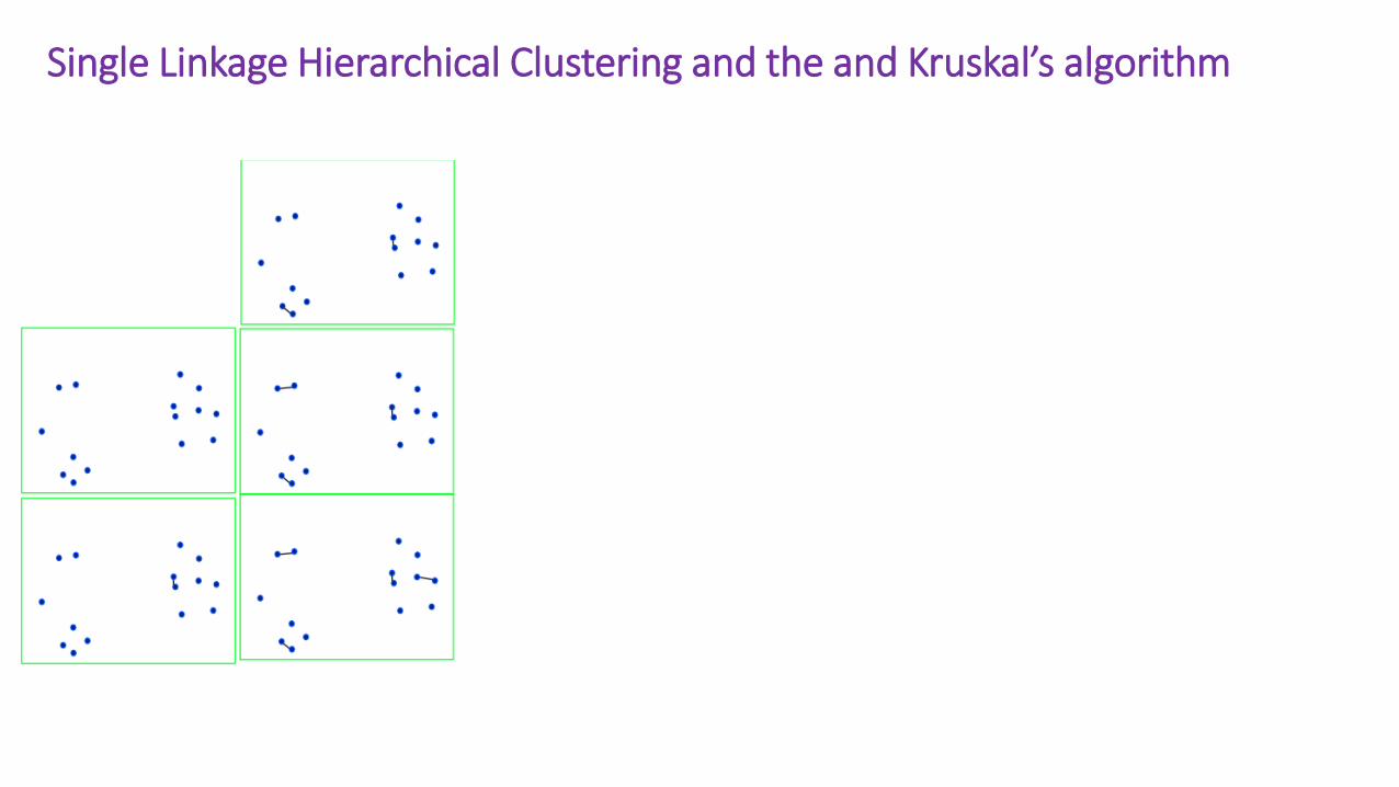
Recall: Single Linkage Hierarchical Clustering and the ɛ- Neighborhood Graph

Every point is a connected component

When ɛ is a little larger we start some clusters starts to get form

When ɛ is even larger we havefew clusters

As the clusters get larger and larger

At some point all points become a par to of a single cluster

Consider the connected components of the ɛ-neighborhood graph as we continuously increase ɛ from zero to infinity.

Suppose that we are given a set of points 𝑋 = 𝑝1, 𝑝2, … , 𝑝𝑛 in 𝑅𝑑 with a distance function 𝑑 defined one them.

Every point is a connected component

When ɛ is a little larger some clusters start to get form

When ɛ is even larger we havefew clusters

As the clusters get larger and larger

At some point all points become a par to of a single cluster

Recall: Single Linkage Hierarchical Clustering and the ɛ- Neighborhood Graph

Consider the connected components of the ɛ-neighborhood graph as we continuously increase ɛ from zero to infinity.

Suppose that we are given a set of points 𝑋 = 𝑝1, 𝑝2, … , 𝑝𝑛 in 𝑅𝑑 with a distance function 𝑑 defined one them.

Every point is a connected component

When ɛ is even larger we havefewer clusters

At some point all points become a par to of a single cluster

When ɛ is a little larger some clusters start to get form

Recall: Single Linkage Hierarchical Clustering and the ɛ- Neighborhood Graph

Consider the connected components of the ɛ-neighborhood graph as we continuously increase ɛ from zero to infinity.

Suppose that we are given a set of points 𝑋 = 𝑝1, 𝑝2, … , 𝑝𝑛 in 𝑅𝑑 with a distance function 𝑑 defined one them.

Every point is a connected component

When ɛ is large enough all points become a part of a single cluster

When ɛ is even larger we havefewer clusters

When ɛ is a little larger some clusters start to get form

Recall: Single Linkage Hierarchical Clustering and the ɛ- Neighborhood Graph

Single Linkage Hierarchical Clustering and the and Kruskal’s algorithm

Single Linkage Hierarchical Clustering and the and Kruskal’s algorithm

Single Linkage Hierarchical Clustering and the and Kruskal’s algorithm

Single Linkage Hierarchical Clustering and the and Kruskal’s algorithm

Single Linkage Hierarchical Clustering and the and Kruskal’s algorithm

Single Linkage Hierarchical Clustering and the and Kruskal’s algorithm

Single Linkage Hierarchical Clustering and the and Kruskal’s algorithm

Single Linkage Hierarchical Clustering and the and Kruskal’s algorithm

Single Linkage Hierarchical Clustering and the and Kruskal’s algorithm

Relationship between 0-persistent homology and single linkage clustering

Essentially dendrogram of a data set in the single linkage clustering at a specific distance ε and the 0-barcode of a data set at a certain max distance encode the exact same information (just represented differently).

Weighted graph -> distance matrix using Dijekstra algorithm -> 0-barcode

0-barcode of a weighted graph

Higher dimensional barcodes

1-barcodes-examples

Persistence Diagram of a scalar function

1-barcodes-examples

Persistence Diagram of a scalar function

1-barcodes-examples