an introduction to parallel programming · central processing unit ... executed. (the boss)...

The University of Adelaide, School of Computer Science 4 March 2015

Chapter 2 — Instructions: Language of the Computer 1

1Copyright © 2010, Elsevier Inc. All rights Reserved

Chapter 2

Parallel Hardware and Parallel Software

An Introduction to Parallel ProgrammingPeter Pacheco


Roadmap

Some background Modifications to the von Neumann model Parallel hardware Parallel software Input and output Performance Parallel program design Writing and running parallel programs Assumptions

# Chapter S

ubtitle



3

SOME BACKGROUND

Copyright © 2010, Elsevier Inc. All rights Reserved

4

Serial hardware and software


input

output

programs

Computer runs one

program at a time.




The von Neumann Architecture# C

hapter Subtitle

Figure 2.1

6

Main memory

This is a collection of locations, each of which is capable of storing both instructions and data.

Every location consists of an address, which is used to access the location, and the contents of the location.




7

Central processing unit (CPU)

Divided into two parts.

Control unit - responsible for deciding which instruction in a program should be executed. (the boss)

Arithmetic and logic unit (ALU) -responsible for executing the actual instructions. (the worker)


add 2+2

8

Key terms

Register – very fast storage, part of the CPU.

Program counter – stores address of the next instruction to be executed.

Bus – wires and hardware that connects the CPU and memory.





memory

CPU

fetch/read


memory

CPU

write/store



11

von Neumann bottleneck


12

An operating system “process”

An instance of a computer program that is being executed.

Components of a process: The executable machine language program.

A block of memory.

Descriptors of resources the OS has allocated to the process.

Security information.

Information about the state of the process.




13

Multitasking

Gives the illusion that a single processor system is running multiple programs simultaneously.

Each process takes turns running. (time slice)

After its time is up, it waits until it has a turn again. (blocks)


14

Threading

Threads are contained within processes.

They allow programmers to divide their programs into (more or less) independent tasks.

The hope is that when one thread blocks because it is waiting on a resource, another will have work to do and can run.




15

A process and two threads


Figure 2.2

the “master” thread

starting a thread

Is called forking

terminating a thread

Is called joining

16

MODIFICATIONS TO THE VON NEUMANN MODEL




17

Basics of caching

A collection of memory locations that can be accessed in less time than some other memory locations.

A CPU cache is typically located on the same chip, or one that can be accessed much faster than ordinary memory.


18

Principle of locality

Accessing one location is followed by an access of a nearby location.

Spatial locality – accessing a nearby location.

Temporal locality – accessing in the near future.




19

Principle of locality


float z[1000];

…

sum = 0.0;

for (i = 0; i < 1000; i++)

sum += z[i];

20

Levels of Cache


L1

L2

L3

smallest & fastest

largest & slowest



21

Cache hit


L1

L2

L3

x sum

y z total

A[ ] radius r1 center

fetch x

22

Cache miss


L1

L2

L3

y sum

r1 z total

A[ ] radius center

fetch x x

main

memory



23

Issues with cache

When a CPU writes data to cache, the value in cache may be inconsistent with the value in main memory.

Write-through caches handle this by updating the data in main memory at the time it is written to cache.

Write-back caches mark data in the cache as dirty. When the cache line is replaced by a new cache line from memory, the dirtyline is written to memory.


24

Cache mappings

Full associative – a new line can be placed at any location in the cache.

Direct mapped – each cache line has a unique location in the cache to which it will be assigned.

n-way set associative – each cache line can be place in one of n different locations in the cache.




25

n-way set associative

When more than one line in memory can be mapped to several different locations in cache we also need to be able to decide which line should be replaced or evicted.


x

26

Example


Table 2.1: Assignments of a 16-line main memory to a 4-line cache



27

Caches and programs


28

Virtual memory (1)

If we run a very large program or a program that accesses very large data sets, all of the instructions and data may not fit into main memory.

Virtual memory functions as a cache for secondary storage.




29

Virtual memory (2)

It exploits the principle of spatial and temporal locality.

It only keeps the active parts of running programs in main memory.


30

Virtual memory (3)

Swap space - those parts that are idle are kept in a block of secondary storage.

Pages – blocks of data and instructions. Usually these are relatively large.

Most systems have a fixed page size that currently ranges from 4 to 16 kilobytes.




31

Virtual memory (4)


program A

program B

program C

main memory

32

Virtual page numbers

When a program is compiled its pages are assigned virtual page numbers.

When the program is run, a table is created that maps the virtual page numbers to physical addresses.

A page table is used to translate the virtual address into a physical address.




33

Page table


Table 2.2: Virtual Address Divided into Virtual Page Number and Byte Offset

34

Translation-lookaside buffer (TLB)

Using a page table has the potential to significantly increase each program’s overall run-time.

A special address translation cache in the processor.




35

Translation-lookaside buffer (2)

It caches a small number of entries (typically 16–512) from the page table in very fast memory.

Page fault – attempting to access a valid physical address for a page in the page table but the page is only stored on disk.


36

Instruction Level Parallelism (ILP)

Attempts to improve processor performance by having multiple processor components or functional units simultaneously executing instructions.




37

Instruction Level Parallelism (2)

Pipelining - functional units are arranged in stages.

Multiple issue - multiple instructions can be simultaneously initiated.


38

Pipelining




39

Pipelining example (1)


Add the floating point numbers 9.87×104 and 6.54×103

40

Pipelining example (2)

Assume each operation takes one nanosecond (10-9 seconds).

This for loop takes about 7000 nanoseconds.




41

Pipelining (3)

Divide the floating point adder into 7 separate pieces of hardware or functional units.

First unit fetches two operands, second unit compares exponents, etc.

Output of one functional unit is input to the next.


42

Pipelining (4)


Table 2.3: Pipelined Addition.

Numbers in the table are subscripts of operands/results.



43

Pipelining (5)

One floating point addition still takes 7 nanoseconds.

But 1000 floating point additions now takes 1006 nanoseconds!


44

Multiple Issue (1)

Multiple issue processors replicate functional units and try to simultaneously execute different instructions in a program.


adder #1 adder #2

z[1]

z[3]

z[2]

z[4]

for (i = 0; i < 1000; i++)z[i] = x[i] + y[i];



45

Multiple Issue (2)

static multiple issue - functional units are scheduled at compile time.

dynamic multiple issue – functional units are scheduled at run-time.


superscalar

46

Speculation (1)

In order to make use of multiple issue, the system must find instructions that can be executed simultaneously.


In speculation, the compiler or the processor makes a guess about an instruction, and then executes the instruction on the basis of the guess.



47

Speculation (2)


z = x + y ;

i f ( z > 0)

w = x ;

e l s e

w = y ;

Z will be

positive

If the system speculates incorrectly,

it must go back and recalculate w = y.

48

Hardware multithreading (1)

There aren’t always good opportunities for simultaneous execution of different threads.

Hardware multithreading provides a means for systems to continue doing useful work when the task being currently executed has stalled. Ex., the current task has to wait for data to be

loaded from memory.




49


Fine-grained - the processor switches between threads after each instruction, skipping threads that are stalled.

Pros: potential to avoid wasted machine time due to stalls.

Cons: a thread that’s ready to execute a long sequence of instructions may have to wait to execute every instruction.


50


Coarse-grained - only switches threads that are stalled waiting for a time-consuming operation to complete.

Pros: switching threads doesn’t need to be nearly instantaneous.

Cons: the processor can be idled on shorter stalls, and thread switching will also cause delays.




51


Simultaneous multithreading (SMT) - a variation on fine-grained multithreading.

Allows multiple threads to make use of the multiple functional units.


52

PARALLEL HARDWAREA programmer can write code to exploit.




53

Flynn’s Taxonomy


SISD

Single instruction stream

Single data stream

(SIMD)

Single instruction stream

Multiple data stream

MISD

Multiple instruction stream

Single data stream

(MIMD)

Multiple instruction stream

Multiple data stream

54

SIMD

Parallelism achieved by dividing data among the processors.

Applies the same instruction to multiple data items.

Called data parallelism.




55

SIMD example


control unit

ALU1 ALU2 ALUn

…

for (i = 0; i < n; i++)x[i] += y[i];

x[1] x[2] x[n]

n data items

n ALUs

56

SIMD

What if we don’t have as many ALUs as data items?

Divide the work and process iteratively.

Ex. m = 4 ALUs and n = 15 data items.


Round3 ALU1 ALU2 ALU3 ALU4

1 X[0] X[1] X[2] X[3]

2 X[4] X[5] X[6] X[7]

3 X[8] X[9] X[10] X[11]

4 X[12] X[13] X[14]



57

SIMD drawbacks

All ALUs are required to execute the same instruction, or remain idle.

In classic design, they must also operate synchronously.

The ALUs have no instruction storage.

Efficient for large data parallel problems, but not other types of more complex parallel problems.


58

Vector processors (1)

Operate on arrays or vectors of data while conventional CPU’s operate on individual data elements or scalars.

Vector registers. Capable of storing a vector of operands and

operating simultaneously on their contents.




59


Vectorized and pipelined functional units. The same operation is applied to each

element in the vector (or pairs of elements).

Vector instructions. Operate on vectors rather than scalars.


60


Interleaved memory. Multiple “banks” of memory, which can be

accessed more or less independently.

Distribute elements of a vector across multiple banks, so reduce or eliminate delay in loading/storing successive elements.

Strided memory access and hardware scatter/gather. The program accesses elements of a vector

located at fixed intervals.




61

Vector processors - Pros

Fast.

Easy to use.

Vectorizing compilers are good at identifying code to exploit.

Compilers also can provide information about code that cannot be vectorized. Helps the programmer re-evaluate code.

High memory bandwidth.

Uses every item in a cache line.


62

Vector processors - Cons

They don’t handle irregular data structures as well as other parallel architectures.

A very finite limit to their ability to handle ever larger problems. (scalability)




63

Graphics Processing Units (GPU)

Real time graphics application programming interfaces or API’s use points, lines, and triangles to internally represent the surface of an object.


64

GPUs

A graphics processing pipeline converts the internal representation into an array of pixels that can be sent to a computer screen.

Several stages of this pipeline (called shader functions) are programmable. Typically just a few lines of C code.




65

GPUs

Shader functions are also implicitly parallel, since they can be applied to multiple elements in the graphics stream.

GPU’s can often optimize performance by using SIMD parallelism.

The current generation of GPU’s use SIMD parallelism. Although they are not pure SIMD systems.


66

MIMD

Supports multiple simultaneous instruction streams operating on multiple data streams.

Typically consist of a collection of fully independent processing units or cores, each of which has its own control unit and its own ALU.




67

Shared Memory System (1)

A collection of autonomous processors is connected to a memory system via an interconnection network.

Each processor can access each memory location.

The processors usually communicate implicitly by accessing shared data structures.


68

Shared Memory System (2)

Most widely available shared memory systems use one or more multicore processors. (multiple CPU’s or cores on a single chip)




69

Shared Memory System


Figure 2.3

70

UMA multicore system


Figure 2.5

Time to access all

the memory locations

will be the same for

all the cores.



71

NUMA multicore system


Figure 2.6A memory location a core is directly connected to can be accessed faster than a memory location that must be accessed through another chip.

72

Distributed Memory System

Clusters (most popular) A collection of commodity systems.

Connected by a commodity interconnection network.

Nodes of a cluster are individual computations units joined by a communication network.


a.k.a. hybrid systems



73

Distributed Memory System


Figure 2.4

74

Interconnection networks

Affects performance of both distributed and shared memory systems.

Two categories: Shared memory interconnects

Distributed memory interconnects




75

Shared memory interconnects

Bus interconnect A collection of parallel communication wires

together with some hardware that controls access to the bus.

Communication wires are shared by the devices that are connected to it.

As the number of devices connected to the bus increases, contention for use of the bus increases, and performance decreases.


76

Shared memory interconnects

Switched interconnect Uses switches to control the routing of data

among the connected devices.

Crossbar – Allows simultaneous communication among

different devices.

Faster than buses.

But the cost of the switches and links is relatively high.





Figure 2.7

(a)

A crossbar switch connecting 4 processors (Pi) and 4 memory modules (Mj)

(b)

Configuration of internal switches in a crossbar

(c) Simultaneous memory accesses by the processors

78

Distributed memory interconnects

Two groups Direct interconnect

Each switch is directly connected to a processor memory pair, and the switches are connected to each other.

Indirect interconnect Switches may not be directly connected to a

processor.




79

Direct interconnect


Figure 2.8

ring toroidal mesh

80

Bisection width

A measure of “number of simultaneous communications” or “connectivity”.

How many simultaneous communications can take place “across the divide” between the halves?




81

Two bisections of a ring


Figure 2.9

82

A bisection of a toroidal mesh


Figure 2.10



83

Definitions

Bandwidth The rate at which a link can transmit data.

Usually given in megabits or megabytes per second.

Bisection bandwidth A measure of network quality.

Instead of counting the number of links joining the halves, it sums the bandwidth of the links.


84

Fully connected network

Each switch is directly connected to every other switch.


Figure 2.11

bisection width = p2/4



85

Hypercube

Highly connected direct interconnect.

Built inductively: A one-dimensional hypercube is a fully-

connected system with two processors.

A two-dimensional hypercube is built from two one-dimensional hypercubes by joining “corresponding” switches.

Similarly a three-dimensional hypercube is built from two two-dimensional hypercubes.


86

Hypercubes


Figure 2.12

one- three-dimensionaltwo-



87

Indirect interconnects

Simple examples of indirect networks: Crossbar

Omega network

Often shown with unidirectional links and a collection of processors, each of which has an outgoing and an incoming link, and a switching network.


88

A generic indirect network


Figure 2.13



89

Crossbar interconnect for distributed memory


Figure 2.14

90

An omega network


Figure 2.15



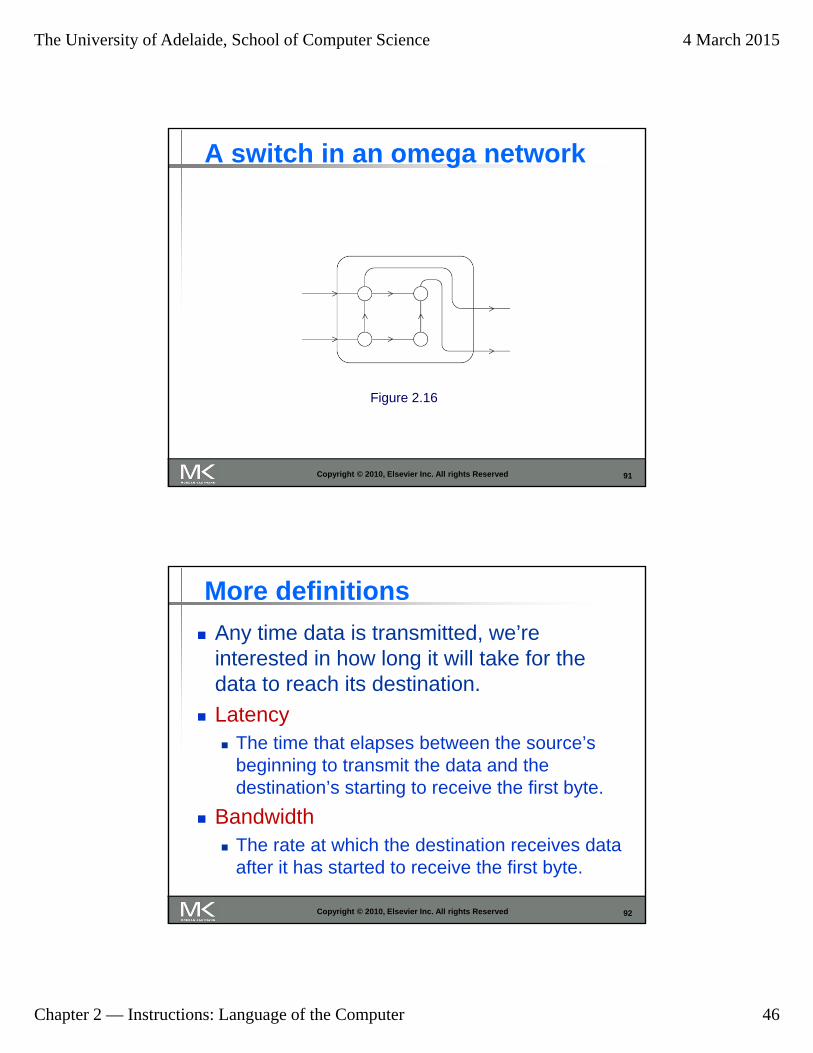
91

A switch in an omega network


Figure 2.16

92

More definitions

Any time data is transmitted, we’re interested in how long it will take for the data to reach its destination.

Latency The time that elapses between the source’s

beginning to transmit the data and the destination’s starting to receive the first byte.

Bandwidth The rate at which the destination receives data

after it has started to receive the first byte.





Message transmission time = l + n / b

latency (seconds)

bandwidth (bytes per second)

length of message (bytes)

94

Cache coherence

Programmers have no control over caches and when they get updated.


Figure 2.17

A shared memory system with two cores and two caches



95

Cache coherence


x = 2; /* shared variable */

y0 privately owned by Core 0y1 and z1 privately owned by Core 1

y0 eventually ends up = 2y1 eventually ends up = 6z1 = ???

96

Snooping Cache Coherence

The cores share a bus .

Any signal transmitted on the bus can be “seen” by all cores connected to the bus.

When core 0 updates the copy of x stored in its cache it also broadcasts this information across the bus.

If core 1 is “snooping” the bus, it will see that x has been updated and it can mark its copy of x as invalid.




97

Directory Based Cache Coherence

Uses a data structure called a directorythat stores the status of each cache line.

When a variable is updated, the directory is consulted, and the cache controllers of the cores that have that variable’s cache line in their caches are invalidated.


98

PARALLEL SOFTWARE




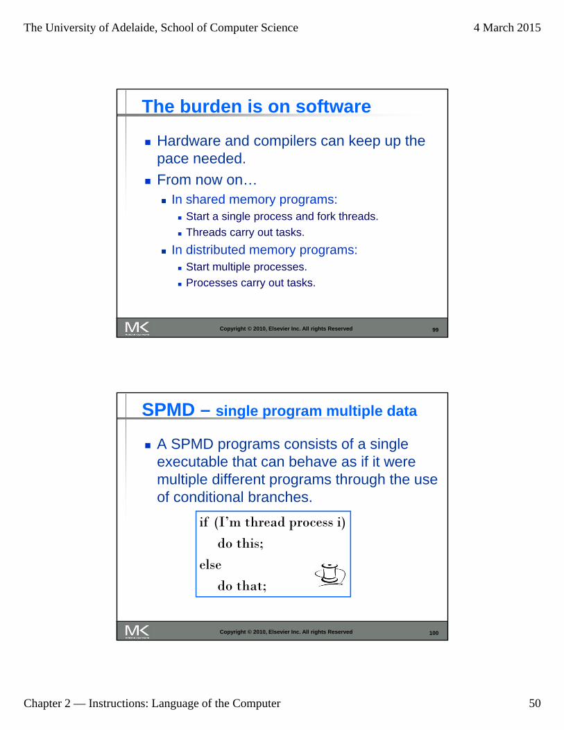
99

The burden is on software

Hardware and compilers can keep up the pace needed.

From now on… In shared memory programs:

Start a single process and fork threads.

Threads carry out tasks.

In distributed memory programs: Start multiple processes.

Processes carry out tasks.


100

SPMD – single program multiple data

A SPMD programs consists of a single executable that can behave as if it were multiple different programs through the use of conditional branches.


if (I’m thread process i)do this;

elsedo that;



101

Writing Parallel Programs


double x[n], y[n];…for (i = 0; i < n; i++)

x[i] += y[i];

1. Divide the work among theprocesses/threads

(a) so each process/threadgets roughly the same amount of work

(b) and communication isminimized.

2. Arrange for the processes/threads to synchronize.

3. Arrange for communication among processes/threads.

102

Shared Memory

Dynamic threads Master thread waits for work, forks new

threads, and when threads are done, they terminate

Efficient use of resources, but thread creation and termination is time consuming.

Static threads Pool of threads created and are allocated

work, but do not terminate until cleanup.

Better performance, but potential waste of system resources.




103

Nondeterminism


. . .printf ( "Thread %d > my_val = %d\n" ,

my_rank , my_x ) ;. . .

Thread 0 > my_val = 7

Thread 1 > my_val = 19Thread 1 > my_val = 19

Thread 0 > my_val = 7

104

Nondeterminism


my_val = Compute_val ( my_rank ) ;x += my_val ;



105

Nondeterminism

Race condition

Critical section

Mutually exclusive

Mutual exclusion lock (mutex, or simply lock)


my_val = Compute_val ( my_rank ) ;Lock(&add_my_val_lock ) ;x += my_val ;Unlock(&add_my_val_lock ) ;

106

busy-waiting


my_val = Compute_val ( my_rank ) ;i f ( my_rank == 1)

whi l e ( ! ok_for_1 ) ; /* Busy−wait loop */x += my_val ; /* Critical section */i f ( my_rank == 0)

ok_for_1 = true ; /* Let thread 1 update x */



107

message-passing


char message [ 1 0 0 ] ;. . .my_rank = Get_rank ( ) ;i f ( my_rank == 1) {

sprintf ( message , "Greetings from process 1" ) ;Send ( message , MSG_CHAR , 100 , 0 ) ;

} e l s e i f ( my_rank == 0) {Receive ( message , MSG_CHAR , 100 , 1 ) ;printf ( "Process 0 > Received: %s\n" , message ) ;

}

108

Partitioned Global Address Space Languages


shared i n t n = . . . ;shared double x [ n ] , y [ n ] ;private i n t i , my_first_element , my_last_element ;my_first_element = . . . ;my_last_element = . . . ;/ * Initialize x and y */. . .f o r ( i = my_first_element ; i <= my_last_element ; i++)

x [ i ] += y [ i ] ;



109

Input and Output

In distributed memory programs, only process 0 will access stdin. In shared memory programs, only the master thread or thread 0 will access stdin.

In both distributed memory and shared memory programs all the processes/threads can access stdout and stderr.


110

Input and Output

However, because of the indeterminacy of the order of output to stdout, in most cases only a single process/thread will be used for all output to stdout other than debugging output.

Debug output should always include the rank or id of the process/thread that’s generating the output.




111

Input and Output

Only a single process/thread will attempt to access any single file other than stdin, stdout, or stderr. So, for example, each process/thread can open its own, private file for reading or writing, but no two processes/threads will open the same file.


112

PERFORMANCE




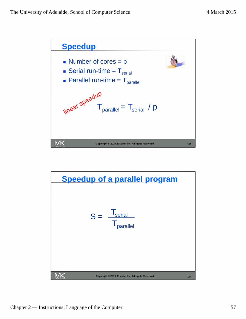
113

Speedup

Number of cores = p

Serial run-time = Tserial

Parallel run-time = Tparallel


Tparallel = Tserial / p

114

Speedup of a parallel program


Tserial

Tparallel

S =



115

Efficiency of a parallel program


E =

Tserial

TparallelS

p =

p =

Tserial

p Tparallel.

116

Speedups and efficiencies of a parallel program




117

Speedups and efficiencies of parallel program on different problem sizes


118

Speedup




119

Efficiency


120

Effect of overhead


Tparallel = Tserial / p + Toverhead



121

Amdahl’s Law

Unless virtually all of a serial program is parallelized, the possible speedup is going to be very limited — regardless of the number of cores available.


122

Example

We can parallelize 90% of a serial program.

Parallelization is “perfect” regardless of the number of cores p we use.

Tserial = 20 seconds

Runtime of parallelizable part is


0.9 x Tserial / p = 18 / p



123

Example (cont.)

Runtime of “unparallelizable” part is

Overall parallel run-time is


0.1 x Tserial = 2

Tparallel = 0.9 x Tserial / p + 0.1 x Tserial = 18 / p + 2

124

Example (cont.)

Speed up


0.9 x Tserial / p + 0.1 x Tserial

Tserial

S = =18 / p + 2

20



125

Scalability

In general, a problem is scalable if it can handle ever increasing problem sizes.

If we increase the number of processes/threads and keep the efficiency fixed without increasing problem size, the problem is strongly scalable.

If we keep the efficiency fixed by increasing the problem size at the same rate as we increase the number of processes/threads, the problem is weakly scalable.


126

Taking Timings

What is time?

Start to finish?

A program segment of interest?

CPU time?

Wall clock time?




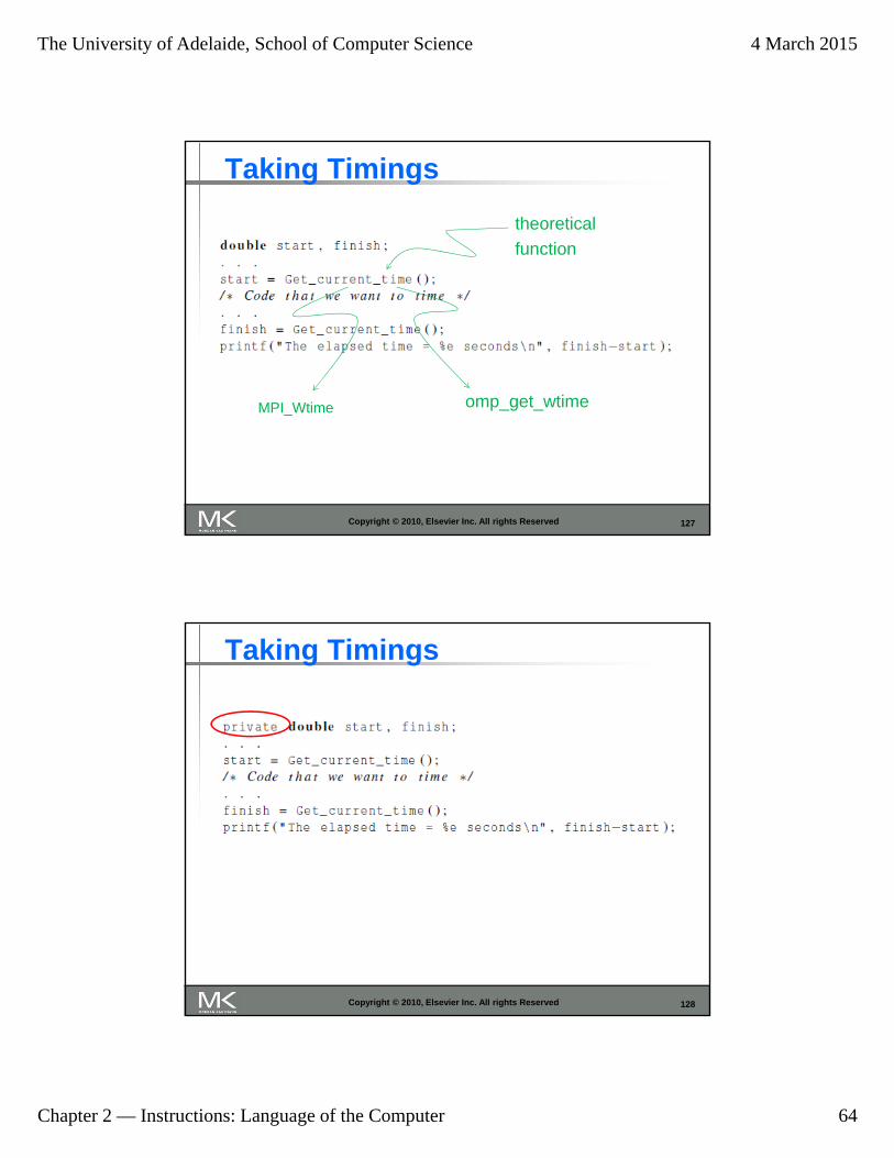
127

Taking Timings


theoretical

function

MPI_Wtime omp_get_wtime

128

Taking Timings




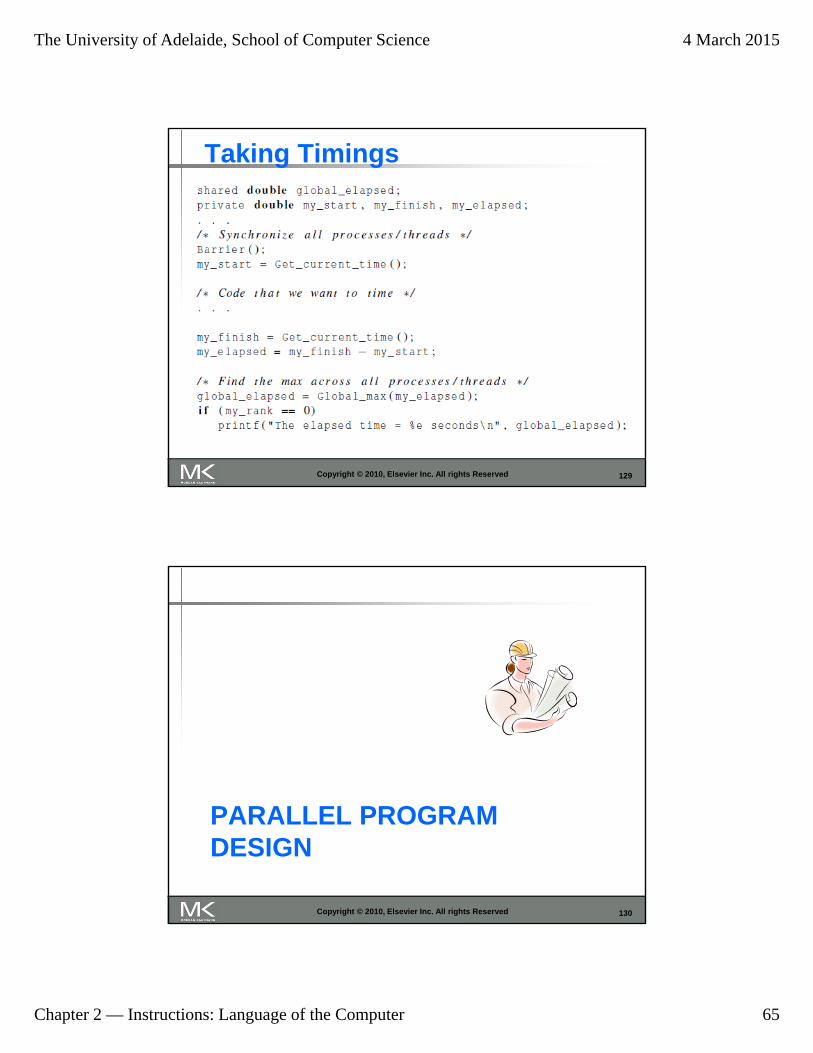
129

Taking Timings


130

PARALLEL PROGRAMDESIGN




131

Foster’s methodology

1. Partitioning: divide the computation to be performed and the data operated on by the computation into small tasks.

The focus here should be on identifying tasks that can be executed in parallel.


132


2. Communication: determine what communication needs to be carried out among the tasks identified in the previous step.




133


3. Agglomeration or aggregation: combine tasks and communications identified in the first step into larger tasks.

For example, if task A must be executed before task B can be executed, it may make sense to aggregate them into a single composite task.


134


4. Mapping: assign the composite tasks identified in the previous step to processes/threads.

This should be done so that communication is minimized, and each process/thread gets roughly the same amount of work.




135

Example - histogram

1.3,2.9,0.4,0.3,1.3,4.4,1.7,0.4,3.2,0.3,4.9,2.4,3.1,4.4,3.9,0.4,4.2,4.5,4.9,0.9


136

Serial program - input

1. The number of measurements: data_count

2. An array of data_count floats: data

3. The minimum value for the bin containing the smallest values: min_meas

4. The maximum value for the bin containing the largest values: max_meas

5. The number of bins: bin_count




137

Serial program - output

1. bin_maxes : an array of bin_count floats

2. bin_counts : an array of bin_count ints


138

First two stages of Foster’s Methodology




139

Alternative definition of tasks and communication


140

Adding the local arrays




141

Concluding Remarks (1)

Serial systems The standard model of computer hardware

has been the von Neumann architecture.

Parallel hardware Flynn’s taxonomy.

Parallel software We focus on software for homogeneous MIMD

systems, consisting of a single program that obtains parallelism by branching.

SPMD programs.


142


Input and Output We’ll write programs in which one process or

thread can access stdin, and all processes can access stdout and stderr.

However, because of nondeterminism, except for debug output we’ll usually have a single process or thread accessing stdout.




143


Performance Speedup

Efficiency

Amdahl’s law

Scalability

Parallel Program Design Foster’s methodology


an introduction to parallel programming · central processing unit ... executed. (the boss)...

Documents