An Introduction to Network

Information Theory with

Slepian-Wolf and Gaussian

Examples By J. Howell

1. What is Network Information Theory?

2. Slepian-Wolf

3. Slepian-Wolf Theorem

4. Slepian-Wolf Theorem Proof

5. Gaussian Broadcast Channels

6. Converse for Gaussian Broadcast Channel

7. Gaussian Interference Channels

8. Gaussian Two Way Channels

Bibliography

What is Network Information Theory?

Before we define Network Information Theory it would be best if we first define Information

Theory. Information Theory is the branch of probability theory that includes the application

of communication systems. This branch of mathematics and computer science was invented

in 1948 by C.E. Shannon along with other communication scientist studying statistical

structures of electrical communication equipment.

Figure: C.E. Shannon

Shannon considered communication system architecture (point to point) where a sender

wishes to communicate a symbol source sequence Uk to a receiver over a noisy channel. The

source sequence is mapped by an encoder into an n- symbol input sequence Xn (Uk) and

received channel output sequence in Yn. (Figure below borrowed from Network Information

Theory Abbas El Gamal Young-Han Kim)

So again we pose the question, what is Network Information Theory? Network Information

Theory considers the information carrying capacity of a network. We have a system with

multiple senders and receivers containing many new elements in the communication

problems such as interference, cooperation and feedback. It involves the fundamental limits

of communication and Information Theory in networks with multiple senders and receivers

and optimal coding techniques and protocols which achieve these limits.

It extends Shannon’s point-to-point information theory to networks with several sources and

destinations. (Diagram below borrowed from Elements of Network Information Theory

Abbas El Gamal and Young-Han Kim)

An important goal is to characterize the capacity region or optimal rate which is the set rate

of the ordered list of elements in which there exist codes with reliable transmissions. These

rates of tuples are known to be achievable. Although a complete theory is yet to be

developed and the characterization of the regions of capacity is generally a difficult problem

there have been positive results for multiple classes of networks.

Computer networks are examples of large communication networks. Even within a lone

computer there are various computers that talk to each other. These large networks coupled

with the advent of the internet and supported by advancements in semiconductor technology,

error correction, compression, computer science and signal processing revived an interest in

a subject which was somewhat dormant through the period from the mid 1980’s up to the

mid 1990’s. Since the mid 1990’s there has been a large scale interest in the activities of this

subject. Not only has there been progress made on past problems, there has also been work

dealing with new network models, scaling laws and capacity approximations and fresh

approaches to coding for networks and subjects intersecting information theory and

networking.

In Networking Information Theory successive refinement of information, successive

cancelation decoding, multiple description and network coding are some of the

methodologies expounded and implemented in the real world of networks. A good example

of a multi-users would consist of U stations or users, where U = 1, 2… u, wishing to

communicate with a familiar satellite over a familiar channel, known as a multiple access

channel.

(Below is a figure of a multiple access channel borrowed from Network Information Theory

Thomas M. Cover, Joy A. Thomas)

The questions posed are, what rates of communication are achievable simultaneously? How

do the users cooperate with each other when sending information to the receiver? What are

the limitations of interference among the users placed on the total rate? There are satisfying

answers for the above questions.

Reversing the network we can consider another example, one television station sending

information to U TV receivers. Below diagram is that of a broadcast channel. (Borrowed

from Network Information Theory Thomas M. Cover, Joy A. Thomas)

The questions that arise here are what rates of information are sent to the different receivers?

How does the sender encode information meant for different receivers in a signal that is

common?

The answers are only known in special cases for this contrast channel. There are also other

channels to consider as special cases of general communication network consisting of N

nodes (connection points trying to communicate with one another).

Those channels are the relay channels, two-way channels and interference channels. For

these channels there are only some answers to the questions regarding the coding strategies

and communication rates. Non-deterministic sources are associated with some of the nodes

in the network. If there are independent sources then the nodes sends independent messages.

We also must allow the source to be dependent also.

This brings to light additional questions, with the channel transition function and the

probability distribution; can we transmit these sources over the channel and recover the

sources at the destination with suitable distortion? How can we beneficially use the

dependence to diminish the sum of information transmitted?

We will consider some of these network communication special cases. We will first look at

the problem of source coding when the channels are noiseless and there is no interference. In

these cases the problem is reduced to locating a set of rates that are associated with the

sources in which the required sources are decoded at the destination with a low error

probability.

Slepian-Wolf

We now introduce the Slepian-Wolf source. Slepian and Wolf were two information theory

researchers. (Photos borrowed from https://en.wikipedia.org/wiki/Wikipedia)

David Slepian Jack K. Wolf

David Slepian (June 30, 1923 – November 29, 2007) was an American mathematician born

in Pittsburgh, Pennsylvania. Jack Kein Wolf (March 14, 1935 – May 12, 2011) was an

American researcher in information theory and coding theory and was born in Newark, New

Jersey. Slepian and Wolf worked together to discover a fundamental result in the distributed

source coding.

The Slepian-Wolf source coding problem is the simplest case for source distribution coding.

This involves having two sources that are separately encoded, but decoded at the common

node. This example is shown in the figure below. (Borrowed from

http://www.scholarpedia.org/article/Slepian-Wolf_coding)

For two correlated streams, such systems employ the Slepian-Wolf coding which is a form of

distributed source coding. Compared to an encoder that assumes that the data streams are

independent, the separated encoders can achieve better compression rates by making use of

the fact that the data systems are complementary.

A surprising result is that the Slepian-Wolf coding can achieve the same compression rate as

an optimal single encoder that has all correlated data streams as inputs. Even when the

encoder has access to multiple correlated data streams, the Slepian-Wolf theorem has

practical applications. For example, in order to diminish the complexity of image and video

compression for cell phones, the stream may be encoded separately without reducing the

compression rate.

Slepian-Wolf Theorem

The systems effectiveness is measured by the rates of encoded bits per source symbol of the

compressed data streams which are outputs by the encoders. The Slepian-Wolf Theorem

defines the set of rates that allows the decoder to reconstruct the correlated data streams with

an arbitrarily small probability of error.

Taking another look at the above figure, encoder 1, observes X1 and sends a message to the

decoder that is a number from the set {1, 2, 3, 4 ... 2 nR1}. Encoder 2, which observes X2,

sends a message to the decoder that is a number set {1, 2, 3, 4,…2nR2}. The outputs from the

two encoders are from the inputs to the single decoder. Upon receiving these two inputs, the

decoder outputs two n-vectors X*1 and X*2 which are estimates of X1 and X2.

We are interested in those systems which the probability X*1 does not equal X1 or X*2 does

not equal X2 can be made small as desired by choosing a sufficiently large n.

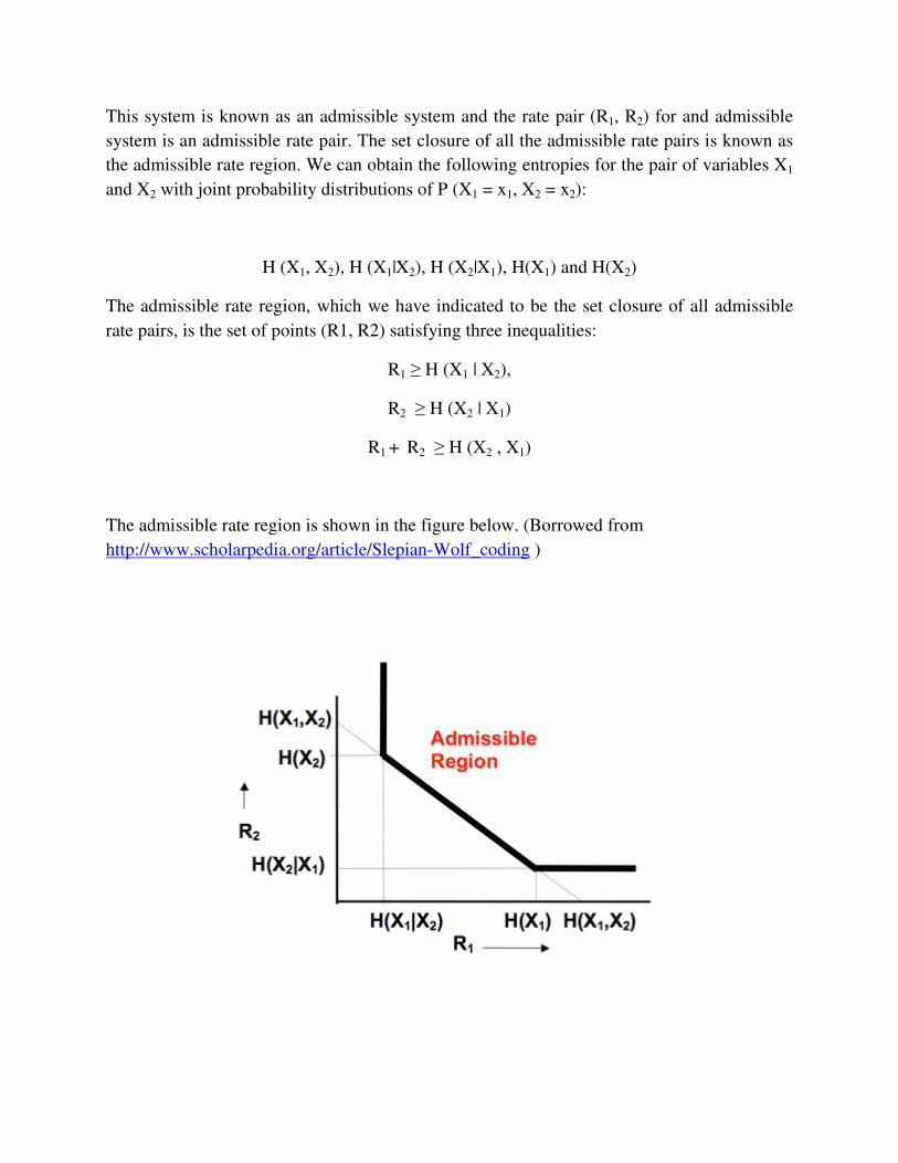
This system is known as an admissible system and the rate pair (R1, R2) for and admissible

system is an admissible rate pair. The set closure of all the admissible rate pairs is known as

the admissible rate region. We can obtain the following entropies for the pair of variables X1

and X2 with joint probability distributions of P (X1 = x1, X2 = x2):

H (X1, X2), H (X1|X2), H (X2|X1), H(X1) and H(X2)

The admissible rate region, which we have indicated to be the set closure of all admissible

rate pairs, is the set of points (R1, R2) satisfying three inequalities:

R1 ≥ H (X1 | X2),

R2 ≥ H (X2 | X1)

R1 + R2 ≥ H (X2 , X1)

The admissible rate region is shown in the figure below. (Borrowed from

http://www.scholarpedia.org/article/Slepian-Wolf_coding )

The importance of the Slepian-Wolf Theorem is realized by the comparison with the entropy

bound for single source compression. Separated encoders that ignore the source correlation

achieve rates only of R1 + R2 ≥ H (X1) + H(X2). Yet with the Slepian-Wolf coding, the

separated encoders are able to achieve their knowledge of the correlation to accomplish the

same rates as an optimal joint encoder, R1 + R2 ≥ H (X1, X2).

Slepian-Wolf Theorem Proof

The condition of the aforementioned three inequalities follows by considering a system

change where the source pair sequences, X1 and X2 are inputs to a separated encoder. The

separated encoder’s output rate must at least equal H(X1, X2), giving: R1 + R2 ≥ H (X1, X2).

If the encoder knows X1 and X2 and the decoder also knows X2, the encoder will need a code

rate at least H (X1|X2) giving R1 ≥ H (X1 | X2). The remaining inequality, R2 ≥ H (X2 | X1)

follows symmetrically.

Showing the adequacy of the three inequalities we consider the rate pair, R1 = H (X1|X2), R2

= H(X2) on the boundary region of the admissible rate region. If R2 = H(X2) then the output

of encoder 2 satisfies the reconstructed X2, so the block diagram shown in the below figure

reduces to the diagram shown in the figure below

(Figures borrowed from http://www.scholarpedia.org/article/Slepian-Wolf_coding)

The initial construction of the admissible system at the rate point R1 = H (X1|X2), R2 = H(X2)

was determined for the statistical model of the correlated source pair, called the twin binary

symmetric source. A twin binary symmetric source is a memory less source with outputs X1

and X2. These outputs are binary random variables with values 0 and 1 represented by:

P (X1 = 0) = P (X1 = 1) = 1/2,

P (X2 = 0| X1 = 1) = P (X2 = 1 | X1 = 0) = p,

P (X2 = 0| X1 = 0) = P (X2 = 1|X1 = 1) = (1 – p)

where p is the parameter satisfying 0 ≤ p ≤ 1. We see that,

P (X2 = 0) = P (X2 = 1) =1/2

Defining h2 (p) = - [p log 2 (p) + (1 – p) log2 (1- p)].

For the twin binary symmetric source we obtain:

H (X1) = 1,

H (X2) = 1,

H (X2|X1) = h2 (p),

H (X1|X2) = h2 (p),

H (X1, X2) = 1 + h2 (p).

For the twin binary symmetric source, the rate point of interest has R1 = H (X1|X2) = h2 (p)

and R2 + H(X2) = 1. To resolve the problem of compressing X1 we can think of the twin

binary symmetric source model as if X1 were passes through a (BSC) binary symmetric

channel with a bit error probability, p, to obtain X2. For large n, a parity code exists for the

BSC with approximately 2n (1-h2 (p))

code words. A decoder that sees the output channel, X2,

will be able to tell which code word was at the channel’s input.

The problem that arises when applying this idea to the source code problem is that the input

to the channel, X1 does not have to be one of the 2n(1-h2(p))

code words of the parity check

code since X1 can be any of the 2n binary n-vectors. Another idea is necessary which comes

from the fact that the co-set decomposition of the group of 2n binary n -vectors are in terms

of the subgroup of the code words. A co-set of this subgroup is formed by taking various

binary n -vector that is not in the subgroup and adding it bit by bit, mod 2 , to each vector in

the subgroup to form a new set of 2n(1-h2(p))

vectors.

Repeat the process choosing a vector to be added, a binary vector that has not been added

before, from either the original subgroup or any previous constructed co-sets. The process is

completed when all 2n binary vectors have surfaced in either the original group or in the co-

sets. The co-sets are now either identical or disjoint and every binary n -vector appears in

only one co-set when considering the subgroup as a co-set.

Given a code block of length n with 2n (1-h2 (p))

code words, we have 2nh2 (p) co-sets since,

2nh2 (p) = 2

n/2

n (1-h2 (p)).

Also the set of vectors in each co-set have similar error correction properties as the original

linear code since the vectors in any co-set are translated versions of the original code words.

These codes are called the co-set code.

After relating this to the problem, X1 must be in one of the co-sets of the code group. When

the source encoder transmits to the decoder the identity of the co-set which includes X1, the

decoder can locate X1 from this knowledge and the knowledge of X2 by using a decoder for

the code’s co-set that worked on the received X2 word. Because there are 2nh2 (p)

co-sets, the

encoder transmits nh2 (p) binary digits. The rate of transmission is h2 (p) = H (X1|X2). The

admissibility of the rate point equals:

R1 = H (X1|X2) = h2 (p) and R2 = H(X2) = 1.

Now the complete admissible rate region follows from time-sharing, wasted bits and

symmetry. We will next consider some Gaussian examples of basic channels of Network

Information Theory.

Gaussian Broadcast Channels

The concept of Gaussian processes is named after Carl Friedrich Gauss (photo borrowed

from http://en.wikipedia.org/wiki/Carl_Friedrich_Gauss) because it is based on the notion of

the normal distribution.

Carl F. Gauss

Carl Gauss (April 30, 1777 – February 23, 1855) was a German

mathematician and physical scientist who contributed to many fields,

including number theory, algebra, statistics, analysis, differential

geometry, geodesy ( a branch of applied mathematics and earth

science), geophysics, electrostatics, astronomy and optics. He was

sometimes referred to as the prince of mathematicians, or the

foremost mathematician and the greatest mathematician since

antiquity. Gauss is ranked as one of our history’s most influential mathematicians. He

referred to mathematics as the queen of science.

We will now define the broadcast channel; the broadcast channel is a communication

channel which there is one sender and two or more receivers. The figure below illustrates the

broadcast channel. (Borrowed from Network Information Theory Thomas M. Cover, Joy A.

Thomas)

The simplest example of a broadcast channel would be a radio or television station. The

station wants everyone tuned in to receive the same information. The capacity is Max p(x) and

Mini I(X; Yi). This may be less than the capacity of the worst receiver. The information can

be arranged so that better receivers will receive additional information, thereby producing a

better sound and picture. The worse receiver will continue to receive more basic information.

Since the introduction of High Definition TV it may be required to encode information so

that poor receivers will receive regular TV signals and better receivers will receive the

additional information to obtain the High Definition signal. We assume we have a sender

with a power of P and two receivers, one with Gaussian noise of power N1 and the other with

Gaussian noise of power N2. We also assume N1 < N2, so receiver Y1 is less noisy than

receiver Y2. The model for this channel is Y1 = X + Z1 and Y2 = X + Z2, where Z1 and Z2 are

correlated Gaussian random variables with a variance of N1 and N2 respectively. All

Gaussian broadcast channels belong to the degraded broadcast channel class. The capacity

region of the Gaussian broadcast channel is Yi = Xi + Zi, where i =1, 2, 3… and where Z are

Gaussian random variables with variance N and a mean equal to 0. The signal X = (X1, X2,

… Xn). The power constraint equals:

The Shannon capacity C is determined by maximizing I (x, y) over all the random variables

X such that EX2 ≤ P and is given by,

C = ½ log (1 + P/N) bits per transmission.

The Gaussian broadcast channel is illustrated in the below figure. (Borrowed from Network

Information Theory Thomas M. Cover, Joy A. Thomas)

One output is a degraded version of the other output. All Gaussian broadcast channels are

equal to this type of degraded channel,

Y1 = X + Z1,

Y2 = X+ Z2 = Y1 + Z’2,

where Z1 ~ N (0, N1) and Z’2 ~ N (0, N2 – N1). The capacity region of this channel is given

by:

R1 < C (α P / N1) and R2 < C ((1- α) P / α P + N2 )

where α equals (0 ≤ α ≤ 1).

Converse for Gaussian Broadcast Channel

Since the Gaussian Broadcast Channel’s capacity region is the same as the physically

degraded Gaussian Broadcast Channel, we can prove the converse for the physically

degraded Gaussian Broadcast Channel. Using Fano’s inequality (also known as Fano

converse and the Fano lemma, relates the average information lost in a noisy channel to the

probability of the categorized error.

Derived by Robert Fano professor emeritus of Electrical Engineering and Computer Science

at Massachusetts Institute of Technology.

(Photo borrowed from http://en.wikipedia.org/wiki/Robert_Fano)

Robert Mario Fano

nR1 ≤ I (M1; Yn1 |M2) + n ε n,

nR2 ≤ I (M2; Yn2) + n ε n,

We next need to show that there exist an α ε [0, 1] such that

I (M1: Yn1|M2) ≤ nC (α S1) = nC (α P / N1)

and I (M2; Yn

2) ≤ nC (α S2 / α S2 + 1) = nC (α P / α P + N2),

Consider

I (M2; Yn2) = h(Yn

2) – h(Yn2|M2) ≤ n/2 log (2 πe ( P + N2)) – h (Yn

2 | M2)

Since

n/2 log (2 πe N2) = h (Zn2) = h(Yn

2|M2, Xn) ≤ h (Yn

2 | M2) ≤ h (Yn2) ≤ n/2 log (2 πe ( P +

N2)),

there must exist an α Ɛ [0, 1] such that

h (Yn2|M2) = n/2 log (2 πe ( P + N2)). *

Next we consider

I (M1; Yn1|M

2) = h (Yn1|M2) – h (Yn

1|M1, M2)

= h (Yn1|M2) – h (Yn

1|M1, M2, Xn)

= h (Yn1|M2) – h (Yn

1| – h (Yn1)

= h (Yn1|M2) – n/2 log (2 πe N1).

Now using the conditional entropy we obtain

h (Yn2|M2) = h (Yn

1 + Zn2 | M2)

≥ n/2 log (22h(Yn1 | M2)/n + 22h(Zn2 | M2)/n)

= n/2 log (22h(Yn1 | M2)/n + 2 πe (N2 – N1).

Combining this inequality with the above equation marked with a * implies that

(2 πe (αP + N2) ≥ 22h(Yn1 | M2)/n + 2 πe (N2 – N1).

Thus, h (Yn1|M2) ≤ (n/2 )log (2 πe ( P + N1)) and hence

I (M1; Yn1|M2) ≤ n/2 log (2 πe (αP + N1)) – n/ log (2 πe N1 ) – nC (αP / N1))

This completes the proof. (Proof borrowed from Network Information Theory Thomas M.

Cover, Joy A. Thomas)

.

Gaussian Interference Channels

There are two senders and two receivers with the Gaussian interference channel. Sender 1

wishes to send information to receiver 1. Sender 1 does not care what receiver 2 receives.

The same holds true for sender 2 and receiver 3. Each channel interferes with one another.

The channel is illustrated in the below figure.

Since there is only one receiver for each sender it is not quite a broadcast channel, nor is it a

multiple access channel since each receiver is interested only in what is being sent by the

similar transmitter. We obtain a symmetric interference of,

Y1 = X1 + aX2 + Z1

Y2 = X2 + aX1 + Z2

where Z1 and Z2 are both independent random variables NNNN (0, N). This is one channel that has

not been generally solved even in the Gaussian case. But in the case of high interference, it

can be remarkably shown that the region of the capacity of this channel is the same as if there

were no interference at all. To achieve this, two code books are generated, each having a

power of P and a rate of C (P / N). Each sender then chooses a word from his book and sends

it. Now given interference a, which satisfies C (a 2 P / (P + N)) > C (P / N) the first

transmitter understands perfectly the index of the second transmitter. The index is found by

looking for the code word closest to his received signal.

Once the signal is found it is subtracted from the received waveform that now presents a

clean channel between the first sender and the second sender. The sender’s code book is

searched to locate the closest code word which is then declared the code word that was sent.

Gaussian Two Way Channel

The only difference between the interference channel and the two way channel is that the two

way channel’s sender1 is attached to receiver 2 and sender 2 is attached to receiver 1. This is

shown in the below figure. (Figure borrowed from Network Information Theory Thomas M.

Cover, Joy A. Thomas)

This allows sender1 to use information from receiver 2 symbols previously received to

determine what to send next. The two way channel also introduces another fundamental

condition of Network Information Theory. This condition is called feedback. Feedback

allows the sender to use limited information that each has about the other message to concur

with one another.

The two way channel’s capacity region is not known in general, although Shannon obtained

upper and lower bounds of the region. These two bounds coexist for Gaussian channels and

the region’s capacity is known. The Gaussian two-way channel separates into two

independent channels. We let the powers of transmitters1 and 2 equal P1 and P2 and the noise

variances of the two channels equal N1 and N2.

Then the rates are equal to,

R1 < C (P1 / N1)

R2 < C (P2 / N2)

this can be accomplished by the methods of the interference channel. So with this case we

would generate two code books with rates R1 and R2. Sender1 sends a code word from code

book 1. Receiver 2 receives the sum of the code words sent by two senders plus some noise.

Receiver 2 simply cuts out sender 2 code word which gives him a clean channel from

sender1 (with only the variance N1 noise). So the two way Gaussian channel separates into

two independent Gaussian channels. This is not the general case of the two way channel; in

general there will be a tradeoff between the two senders so that the both of them cannot send

optimal rates simultaneously.

INFORMATION THEORY

Bibliography

Jack K. Wolf and Brian M. Kukoski,. "Slepian-Wolf coding.” 21 October 2011, 04:16

<http://www.scholarpedia.org/article/Slepian-Wolf_coding>

Thomas M. Cover, Joy A. Thomas. Elements of Information Theory. Chapter 14 Network

Information Theory. New York: Wiley-Interscience; 26 August, 1991

“Gaussian Process”. Wikipedia: The Free Encyclopedia. Wikimedia Foundation, Inc. 4 May

2013 at 13:16. Web. 3 May.2012

Gama, E. Abbas and Kim, H. Young. Network Information Theory. New York: Cambridge

University Press ; January 16, 2012

“Robert Fano”. Wikipedia: The Free Encyclopedia. Wikimedia Foundation, Inc. 31 March

2013 at 21:09.. Web. 3 May.2013

“David Slepian”. Wikipedia: The Free Encyclopedia. Wikimedia Foundation, Inc. 07 March

2013 at 21:09. Web. 3 May.2013

“Jack K. Wolf”. Wikipedia: The Free Encyclopedia. Wikimedia Foundation, Inc. 17

February 2013 at 21:09.. Web. 3 May.2012

“Carl F. Gauss”. Wikipedia: The Free Encyclopedia. Wikimedia Foundation, Inc. 04 May

2013 at 21:09.. Web. 3 May.2012