an introduction to machine learning - alex smolaalex.smola.org/teaching/pune2007/pune_1.pdf ·...

An Introduction to Machine LearningL1: Basics and Probability Theory

Alexander J. Smola

Statistical Machine Learning ProgramCanberra, ACT 0200 Australia

[email protected]

Tata Institute, Pune, January 2007

Alexander J. Smola: An Introduction to Machine Learning 1 / 47

Overview

L1: Machine learning and probability theoryIntroduction to pattern recognition, classification, regression,novelty detection, probability theory, Bayes rule, inference

L2: Density estimation and Parzen windowsNearest Neighbor, Kernels density estimation, Silverman’srule, Watson Nadaraya estimator, crossvalidation

L3: Perceptron and KernelsHebb’s rule, perceptron algorithm, convergence, featuremaps, kernels

L4: Support Vector estimationGeometrical view, dual problem, convex optimization, kernels

L5: Support Vector estimationRegression, Quantile regression, Novelty detection, ν-trick

L6: Structured EstimationSequence annotation, web page ranking, path planning,implementation and optimization


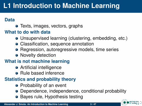
L1 Introduction to Machine Learning

DataTexts, images, vectors, graphs

What to do with dataUnsupervised learning (clustering, embedding, etc.)Classification, sequence annotationRegression, autoregressive models, time seriesNovelty detection

What is not machine learningArtificial intelligenceRule based inference

Statistics and probability theoryProbability of an eventDependence, independence, conditional probabilityBayes rule, Hypothesis testing


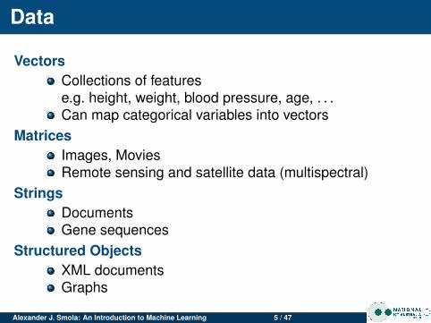
Data

VectorsCollections of featurese.g. height, weight, blood pressure, age, . . .Can map categorical variables into vectors

MatricesImages, MoviesRemote sensing and satellite data (multispectral)

StringsDocumentsGene sequences

Structured ObjectsXML documentsGraphs


Optical Character Recognition


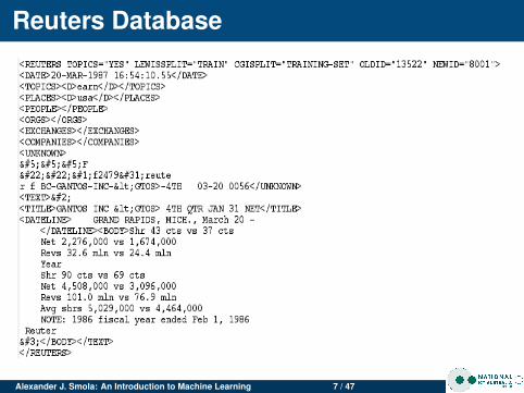
Reuters Database


Faces


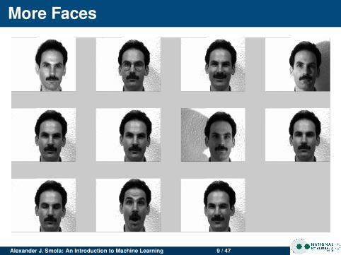
More Faces


Microarray Data


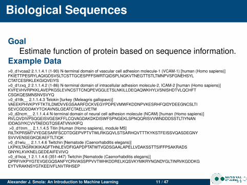
Biological Sequences

GoalEstimate function of protein based on sequence information.

Example Data>0_d1vcaa2 2.1.1.4.1 (1-90) N-terminal domain of vascular cell adhesion molecule-1 (VCAM-1) [human (Homo sapiens)]FKIETTPESRYLAQIGDSVSLTCSTTGCESPFFSWRTQIDSPLNGKVTNEGTTSTLTMNPVSFGNEHSYLCTATCESRKLEKGIQVEIYS>0_d1zxq_2 2.1.1.4.2 (1-86) N-terminal domain of intracellular adhesion molecule-2, ICAM-2 [human (Homo sapiens)]KVFEVHVRPKKLAVEPKGSLEVNCSTTCNQPEVGGLETSLNKILLDEQAQWKHYLVSNISHDTVLQCHFTCSGKQESMNSNVSVYQ>0_d1tlk__ 2.1.1.4.3 Telokin [turkey (Meleagris gallopavo)]VAEEKPHVKPYFTKTILDMDVVEGSAARFDCKVEGYPDPEVMWFKDDNPVKESRHFQIDYDEEGNCSLTISEVCGDDDAKYTCKAVNSLGEATCTAELLVETM>0_d2ncm__ 2.1.1.4.4 N-terminal domain of neural cell adhesion molecule (NCAM) [human (Homo sapiens)]RVLQVDIVPSQGEISVGESKFFLCQVAGDAKDKDISWFSPNGEKLSPNQQRISVVWNDDDSSTLTIYNANIDDAGIYKCVVTAEDGTQSEATVNVKIFQ>0_d1tnm__ 2.1.1.4.5 Titin [Human (Homo sapiens), module M5]RILTKPRSMTVYEGESARFSCDTDGEPVPTVTWLRKGQVLSTSARHQVTTTKYKSTFEISSVQASDEGNYSVVVENSEGKQEAEFTLTIQK>0_d1wiu__ 2.1.1.4.6 Twitchin [Nematode (Caenorhabditis elegans)]LKPKILTASRKIKIKAGFTHNLEVDFIGAPDPTATWTVGDSGAALAPELLVDAKSSTTSIFFPSAKRADSGNYKLKVKNELGEDEAIFEVIVQ>0_d1koa_1 2.1.1.4.6 (351-447) Twitchin [Nematode (Caenorhabditis elegans)]QPRFIVKPYGTEVGEGQSANFYCRVIASSPPVVTWHKDDRELKQSVKYMKRYNGNDYGLTINRVKGDDKGEYTVRAKNSYGTKEEIVFLNVTRHSEP


Graphs


Missing Variables

Incomplete DataMeasurement devices may failE.g. dead pixels on camera, microarray, formsincomplete, . . .Measuring things may be expensivediagnosis for patientsData may be censored

How to fix itClever algorithms (not this course . . . )Simple mean imputationSubstitute in the average from other observationsWorks amazingly well (for starters) . . .


Mini Summary

Data TypesVectors (feature sets, microarrays, HPLC)Matrices (photos, dynamical systems, controllers)Strings (texts, biological sequences)Structured documents (XML, HTML, collections)Graphs (web, gene networks, tertiary structure)

Problems and OpportunitiesData may be incomplete (use mean imputation)Data may come from different sources (adapt model)Data may be biased (e.g. it is much easier to get bloodsamples from university students for cheap).Problem may be ill defined, e.g. “find information.”(get information about what user really needs)Environment may react to intervention(butterfly portfolios in stock markets)


What to do with data

Unsupervised LearningFind clusters of the dataFind low-dimensional representation of the data(e.g. unroll a swiss roll, find structure)Find interesting directions in dataInteresting coordinates and correlationsFind novel observations / database cleaning

Supervised LearningClassification (distinguish apples from oranges)Speech recognitionRegression (tomorrow’s stock value)Predict time seriesAnnotate strings


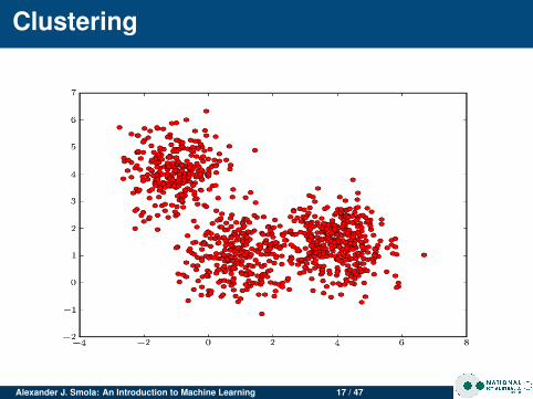
Clustering


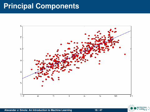
Principal Components


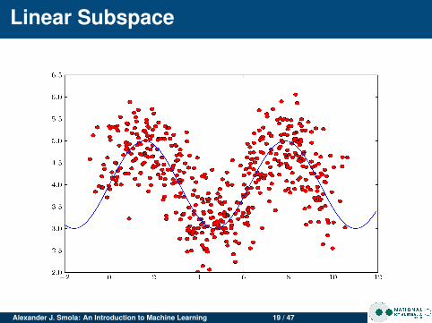
Linear Subspace


Classification

DataPairs of observations (xi , yi) drawn from distributione.g., (blood status, cancer), (credit transactions, fraud),(sound profile of jet engine, defect)

GoalEstimate y ∈ {±1} given x at a new location. Or find afunction f (x) that does the trick.


Regression


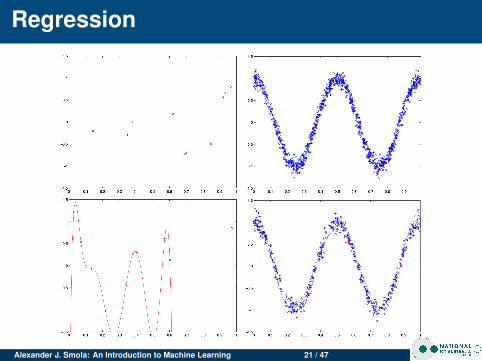
Regression

DataPairs of observations (xi , yi) generated from some jointdistribution Pr(x , y), e.g.,

market index, SP100fab parfameters, yielduser profile, price

TaskEstimate y , given x , such that some loss c(x , y , f (x)) isminimized.

ExamplesQuadratic error between y and f (x), i.e.c(x , y , f (x)) = 1

2(y − f (x))2.Absolute value, i.e., c(x , y , f (x)) = |y − f (x))|.


Annotating Strings


Annotating Audio

GoalPossible meaning of an audio sequenceGive confidence measure

Example (from Australian Prime Minister’s speech)a stray alienAustralian


Novelty Detection

DataObservations xi fromsome P(x), e.g.,

network usagepatternshandwritten digitsalarm sensorsfactory status

TaskFind unusual events,clean database,distinguish typicalexamples.


What Machine Learning is not

LogicIf A meets B and B meets C, does A know C?Rule satisfactionLogical rules from data

Artificial IntelligenceUnderstanding of the worldMeet Sunny from I, RobotGo and get me a bottle of beerRobot need not understand what it is doing.

Biology and NeuroscienceUnderstand the brain by building neural networks?!?Model brain and build good systems with thatGet inspiration from biology but no requirement to buildsystems like that (e.g. jet planes don’t flap wings)


Eliza

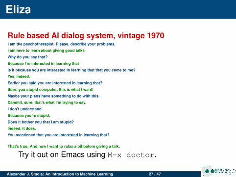
Rule based AI dialog system, vintage 1970I am the psychotherapist. Please, describe your problems.

I am here to learn about giving good talks

Why do you say that?

Because I’m interested in learning that

Is it because you are interested in learning that that you came to me?

Yes, indeed.

Earlier you said you are interested in learning that?

Sure, you stupid computer, this is what I want!

Maybe your plans have something to do with this.

Dammit, sure, that’s what i’m trying to say.

I don’t understand.

Because you’re stupid.

Does it bother you that I am stupid?

Indeed, it does.

You mentioned that you are interested in learning that?

That’s true. And now I want to relax a bit before giving a talk.

Try it out on Emacs using M-x doctor.


How the brain doesn’t work


Mini Summary

Structure ExtractionClusteringLow-dimensional subspacesLow-dimensional representation of data

Novelty DetectionFind typical observations (Joe Sixpack)Find highly unusual ones (oddball)Database cleaning

Supervised LearningRegressionClassificationPreference relationships (recommender systems)


Statistics and Probability Theory

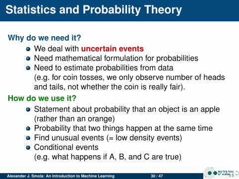
Why do we need it?We deal with uncertain eventsNeed mathematical formulation for probabilitiesNeed to estimate probabilities from data(e.g. for coin tosses, we only observe number of headsand tails, not whether the coin is really fair).

How do we use it?Statement about probability that an object is an apple(rather than an orange)Probability that two things happen at the same timeFind unusual events (= low density events)Conditional events(e.g. what happens if A, B, and C are true)


Probability

Basic IdeaWe have events in a space of possible outcomes. ThenPr(X ) tells us how likely is that an event x ∈ X will occur.

Basic AxiomsPr(X ) ∈ [0, 1] for all X ⊆ X

Pr(X) = 1Pr (∪iXi) =

∑i

Pr(Xi) if Xi ∩ Xj = ∅ for all i 6= j

Simple Corollary

Pr(X ∪ Y ) = Pr(X ) + Pr(Y )− Pr(X ∩ Y )


Example


Multiple Variables

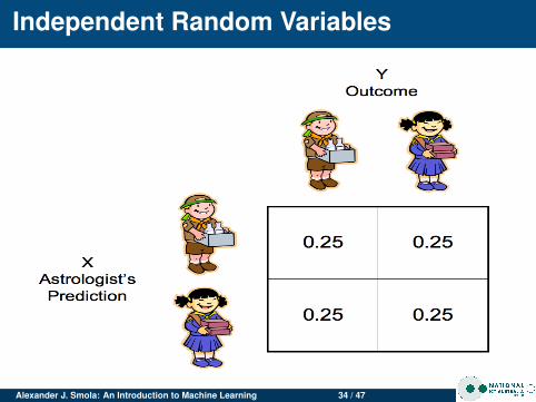
Two SetsAssume that x and y are drawn from a probability measureon the product space of X and Y. Consider the space ofevents (x , y) ∈ X× Y.

IndependenceIf x and y are independent, then for all X ⊂ X and Y ⊂ Y

Pr(X , Y ) = Pr(X ) · Pr(Y ).


Independent Random Variables


Dependent Random Variables


Bayes Rule

Dependence and Conditional ProbabilityTypically, knowing x will tell us something about y (thinkregression or classification). We have

Pr(Y |X ) Pr(X ) = Pr(Y , X ) = Pr(X |Y ) Pr(Y ).

Hence Pr(Y , X ) ≤ min(Pr(X ), Pr(Y )).Bayes Rule

Pr(X |Y ) =Pr(Y |X ) Pr(X )

Pr(Y ).

Proof using conditional probabilities

Pr(X , Y ) = Pr(X |Y ) Pr(Y ) = Pr(Y |X ) Pr(X )


Example

Pr(X ∩ X ′) = Pr(X |X ′) Pr(X ′) = Pr(X ′|X ) Pr(X )


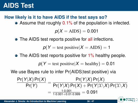
AIDS Test

How likely is it to have AIDS if the test says so?Assume that roughly 0.1% of the population is infected.

p(X = AIDS) = 0.001

The AIDS test reports positive for all infections.

p(Y = test positive|X = AIDS) = 1

The AIDS test reports positive for 1% healthy people.

p(Y = test positive|X = healthy) = 0.01

We use Bayes rule to infer Pr(AIDS|test positive) via

Pr(Y |X ) Pr(X )

Pr(Y )=

Pr(Y |X ) Pr(X )

Pr(Y |X ) Pr(X ) + Pr(Y |X\X ) Pr(X\X )

= 1·0.0011·0.001+0.01·0.999 = 0.091


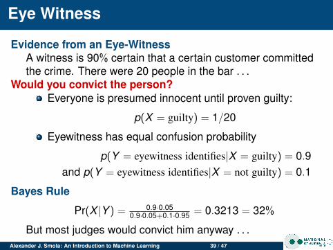
Eye Witness

Evidence from an Eye-WitnessA witness is 90% certain that a certain customer committedthe crime. There were 20 people in the bar . . .

Would you convict the person?Everyone is presumed innocent until proven guilty:

p(X = guilty) = 1/20

Eyewitness has equal confusion probability

p(Y = eyewitness identifies|X = guilty) = 0.9and p(Y = eyewitness identifies|X = not guilty) = 0.1

Bayes Rule

Pr(X |Y ) = 0.9·0.050.9·0.05+0.1·0.95 = 0.3213 = 32%

But most judges would convict him anyway . . .Alexander J. Smola: An Introduction to Machine Learning 39 / 47

Improving Inference

Follow up on the AIDS test:The doctor performs a followup via a conditionallyindependent test which has the following properties:

The second test reports positive for 90% infections.The AIDS test reports positive for 5% healthy people.

Pr(T1, T2|Health) = Pr(T1|Health) Pr(T2|Health).

A bit more algebra reveals (assuming that both tests areindependent): 0.01·0.05·0.999

0.01·0.05·0.999+1·0.9·0.001 = 0.357.Conclusion:

Adding extra observations can improve the confidence of thetest considerably.


Different Contexts

Hypothesis Testing:Is solution A or B better to solve the problem (e.g. inmanufacturing)?Is a coin tainted?Which parameter setting should we use?

Sensor Fusion:Evidence from sensors A and B (AIDS test 1 and 2).We have different types of data.

More Data:We obtain two sets of data — we get more confidentEach observation can be seen as an additional test


Mini Summary

Probability theoryBasic tools of the tradeUse it to model uncertain events

Dependence and IndependenceIndependent events don’t convey any information abouteach other.Dependence is what we exploit for estimationLeads to Bayes rule

TestingPrior probability mattersCombining tests improves outcomesCommon sense can be misleading


Estimating Probabilities from Data

Rolling a dice:Roll the dice many times and count how many times eachside comes up. Then assign empirical probability estimatesaccording to the frequency of occurrence.

P̂r(i) = #occurrences of i#trials

Maximum Likelihood Estimation:Find parameters such that the observations are most likelygiven the current set of parameters.

This does not check whether the parameters are plausible!


Practical Example


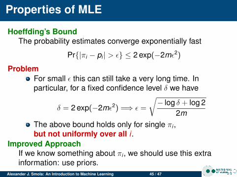
Properties of MLE

Hoeffding’s BoundThe probability estimates converge exponentially fast

Pr{|πi − pi | > ε} ≤ 2 exp(−2mε2)

ProblemFor small ε this can still take a very long time. Inparticular, for a fixed confidence level δ we have

δ = 2 exp(−2mε2) =⇒ ε =

√− log δ + log 2

2mThe above bound holds only for single πi ,but not uniformly over all i .

Improved ApproachIf we know something about πi , we should use this extrainformation: use priors.


Mini Summary

Probability EstimatesFor discrete events, just count occurrences.Results can be bad if only few data available.

Maximum LikelihoodFind parameters which maximize the joint probability ofthe data occurring.Result is not a “real” probability.Optimization gives constrained problem, solve usingLagrange function.

Big Guns: Hoeffding and friendsUse uniform convergence and tail boundsExponential convergence for fixed scaleOnly sublinear convergence, when fixed confidence.


Summary

DataVectors, matrices, strings, graphs, . . .

What to do with dataUnsupervised learning (clustering, embedding, etc.),Classification, sequence annotation, Regression, . . .

Random VariablesDependence, Bayes rule, hypothesis testing

Estimating ProbabilitiesMaximum likelihood, convergence, . . .
