An Introduction to Knot Theory

Matt Skerritt (c9903032)

June 27, 2003

1 Introduction

A knot, mathematically speaking, is a closed curve sitting in three dimensional space that does notintersect itself. Intuitively if we were to take a piece of string, cord, or the like, tie a knot in it andthen glue the loose ends together, we would have a knot. It should be impossible to untangle the knotwithout cutting the string somewhere. The use of the word ‘should’ here is quite deliberate, however.It is possible, if we have not tangled the string very well, that we will be able to untangle the mess wecreated and end up with just a circle of string. Of course, this circle of string still fits the definitionof a closed curve sitting in three dimensional space and so is still a knot, but it’s not very interesting.We call such a knot the trivial knot or the unknot.

Knots come in many shapes and sizes from small and simple like the unknot through to large andtangled and messy, and beyond (and everything in between). The biggest questions to a knot theoristare “are these two knots the same or different” or even more importantly “is there an easy way to tellif two knots are the same or different”. This is the heart of knot theory. Merely looking at two tangledmesses is almost never sufficient to tell them apart, at least not in any interesting cases. Consider thefollowing four images for example.

It might be surprising to find out that the four images only show two different knots. The questionis which ones are the same? Are three of them the same and one different, or are there two pairs ofidentical knots? A better question is how can we work out which are the same and which are different?Unless we are particularly imaginative and/or good at visualisation simply looking at the images won’thelp. Even if visualisation could give us the answer, it wouldn’t help us to impart our knowledge toanother person, we’d need something external to ourselves for that, and preferably something moreconcrete than just saying “this is the answer”. We could perhaps try using string to create the knotsshown in the images, and manipulate them to see which we could make the same. This method is veryintuitive (not to mention a not unpleasant way of spending time) although it requires time, patienceand tenacity (particularly in the case of very tangled up messes of knots).

The biggest problem however, with both these methods and others as well, is that they are subjectto circumstance. Maybe we can see the answer, or maybe we can’t. Maybe we’re clever or luckyenough with the string to get an answer, or maybe we’re not. There is no mathematical patternto this, just circumstance. Furthermore, if we have two knots and, using whatever techniques wefind appropriate, not succeed in turning one into the other (or in turning them both into somethingsomething identical) then we have no useful information. We have not shown that the two knots are

1

different, but only that we cannot make them be the same. This puts a new light on our previousquestions of telling knots apart. We at least have a chance of showing that two knots are the same,but how to we conclusively show that two tangled messes can never be manipulated to be the same?

This is what knot theory is about, and this is what we will be discussing in the following pages.We will formalise how we describe and present (ie draw) knots and how we manipulate them. We willlook briefly at joining knots together, and at knots that have multiple strings. But most importantly,we will introduce the tools that allows us to show that knots are different, the knot invariants, andwill examine and discuss several of these.

1.1 Knot Projections

Three dimensional space is difficult to model effectively on paper, so when looking at knots, we usuallyuse a two dimensional image of the knot. Since knots themselves are 1 dimensional objects, they arenot difficult to draw on a plane, so long as we take care to note, when strings cross, which string isabove and which string is below. We call this a projection of a knot. Two such projections are shownbelow in Table 1, along with a corresponding“three dimensional” representation of the same knot.The first is a projection of the unknot, the second is a projection of what is called the trefoil knot.

Figure 1: The Unknot and the Trefoil

Note the break in some of the lines in the trefoil projection. These are not, in fact, breaks in thestring making up the knot, but a way of showing that the string goes under another string. This ishow we differentiate between the string that is above and and the string that is below. Such a pointon the knot is known as a crossing. So the trefoil projection shown above has, as the name might haveimplied, three crossings.

Each entire unbroken line of a projection is known as a strand of the knot projection. See Figure2 for some examples of strands. The strands are marked in grey, but they are not the only strands ofthe projection in question.

Figure 2: Examples of a strands

If we were to trace our finger around the projection in a single direction, we would pass throughevery crossing twice, once by tracing the uppermost string (the overstrand) and once, later on, whentracing the undermost string (the understrand). When tracing the knot this way, we call a crossingan overcrossing if we are traveling on the overstrand, and an undercrossing if we are traveling onthe understrand. We can give the projection (or, indeed, the knot) an orientation by choosing thedirection in which we trace our finger (or travel) around it. There are only 2 choices. We then draw

2

the projection with arrows indicating the direction of travel. We call a knot with an orientation anoriented knot. An oriented trefoil is shown below in Figure 3.

Figure 3: An Oriented Trefoil Knot

We now have a way of describing knots on paper. The bad news is that a knot projection is notunique to it’s knot. Any knot may have many different projections. If we consider our string analogue,we could look at the knotted string from any direction (above, behind, besides, or some combination)and draw a projection of what we saw. Also, we could manipulate the string, pulling it here, andthere, twisting it around itself etc and draw a projection of the result. So long as we do not cutthe string, any manipulation of the string we do can be undone, returning us to wherever we startedfrom, so we have not changed the knot at all, only made it look different. To complicate matters evenfurther, we consider the “string” of a mathematical knot to be indefinitely shrinkable or stretchable,so our analogue of a knotted string is a little inaccurate; knotted rubber tube might be a little better.Some examples of different projections of the trefoil knot are shown in Figure 4, below, to illustratethis idea.

Figure 4: Two Projections of the Trefoil Knot

Since we are usually dealing with projections of knots, and not three dimensional objects, we needsome rules to formalise these concepts for projections.

1.2 Projection Deformations and Reidemeister Moves

If we deform our now rubber knot in such a way as to not add or remove any crossings, then it shouldbe easy to see that the knot itself has not changed significantly. Such a deformation is called a planarisotopy. It should be pointed out here that although the “rubber” making up the knot is consideredto be indefinitely shrinkable, we still cannot remove part of the knot by infinitely shrinking string, sothat the knot becomes a point. This fits our rubber or string analogy, as we could not remove part ofa knot by pulling the strings of the knot tighter and tighter. Some planar isotopies of the trefoil areshown below.

Figure 5: Planar isotopies of the Trefoil

Planar isotopy only gets us so far. We haven’t accounted for much of what we could do with aphysical knot. So far we have allowed only deformations that do not add or remove crossings. This is

3

clearly unreasonable, as we can twist the string of the knot around itself in any number of imaginableways. So we need some way of modeling this for a projection.

Enter the Reidemeister moves, a set of three transformations that add or remove links to a projec-tion by moving the strings around to produce another projection of the same knot. They are namedafter their creator, Kurt Reidemeister. The first such move, called a Type I Reidemeister move, allowsus to “twist” a single piece of string thereby adding a crossing to the projection, or to remove such atwist.

Figure 6: Type I Reidemeister Move

The second Reidemeister move, called a Type II Reidemeister move, allows us to pull part of a stringeither over or under another string. This will either add, or remove, two crossings.

Figure 7: Type II Reidemeister Move

The last Reidemeister move allows us to move a string that is either above or below another crossingto the other side of that crossing.

Figure 8: Type III Reidemeister Move

In each of these examples, it is assumed that the knot projection presented is only a small partof a larger projection, and that the rest of that projection remains unchanged. It was proven byReidemeister that if two knot projections have a sequence of Reidemeister moves and planar isotopiesthat transform one into the other, then those two projections are of the same knot.

Unfortunately, while this gives us a nice way to show that two knot projections are the same, itdoes not give us a very satisfactory method of telling when two knot projections are different. Anyattempt to show that two projections are distinct would need to show that there is no possible sequenceof Reidemeister moves1 to transform one projection into the other. Such proofs tend to be difficult.2

We will discuss more about identification of distinct knots in Section 2.

1.3 Prime and Composite Knots

If we take two knots, K1 and K2 say, we may produce a new knot by composing the two knots together.We do this by taking a projection of each knot, making sure they don’t overlap at all, and then remove

1and planar isotopies, but it’s simpler to take the planar isotopies as read and only consider the sequences of Reide-meister moves

2In much the same way that mountains tend to be tall

4

a small arc from a each projection. We then create two new arcs, each of which connect one of theendpoints of the break in K1 with one of the endpoints of the break in K2. We denote the new knotK1#K2. The arcs to be removed must be removed from the outside of the projection of the knot theyrepresent. Also the new arcs may not cross each other, nor may they cross either of the original knotprojections. See Figure 9 to see how two trefoil knots can be composed.

−→

Figure 9: Knot Composition

A knot created in such a way from nontrivial knots is called a composite knot. Indeed any knotwhich may be constructed in such a way is a composite knot. The knots that compose to make theknot are called the factor knots of the composite knot. This is very similar to the idea of compositeintegers, and their prime factors. In fact, A knot that cannot be be constructed by composition ofnontrivial knots is known as a prime knot.

We have already shown the existence of at least one composite knot in Figure 9, above. Howeverit remains to be shown whether or not prime knots actually exist; for all we know at the moment,every knot may be able to be constructed by composition of other knots. As it happens prime knotsmost certainly do exist. In fact the trefoil knot presented earlier is a prime knot and although it is byno means obvious, we will not prove this fact here.

The similarity to the integers continues, for if we compose any knot with the unknot, what we endup with is the original knot. This is similar to the integer 1, and is the reason for requiring that acomposite knot is made up of nontrivial factors (for otherwise every knot would be composite withitself and the unknot as factors). And to extend the similarity still, it was shown in 1949 by a mannamed Schubert that the factors of a composite knot are unique.

Much work has gone into tabulating prime knots, and all the prime knots having up to 10 crossingsare known3. The number of prime knots of n crossings is tabulated as follows for n = 1, . . . , 10

Number of Crossings (n) 1 2 3 4 5 6 7 8 9 10

Number of Knots of n crossings 0 0 1 1 2 3 7 21 49 165

The collection of all prime knots of up to seven crossings is presented in Figure 10.As a final note, is should be pointed out that (unlike the integers) it is possible to obtain different

knots by composing the same two knots in different ways. This does not always happen, but is possible.Of course, even if it does happen the different resultant composite knots will both have the same factorknots, even though the composite knots are different.

3The author is of the understanding that all prime knots of up to n crossings are known for some n > 10, which isprobably either 13 or 16. Unfortunately the author cannot find a source to validate exactly which n

5

Figure 10: All Prime Knots of up to 7 crossings

1.4 Links

So far we have only concerned ourselves with knots consisting of one knotted ‘string’. This is fine asfar as it goes, but there is absolutely no reason not to consider knots comprised of multiple, distinct’strings’ all tangled together. Such a thing is called a link. Each “string” of a link is called a componentof the link, and is a closed curve in three dimensional space, just as a knot is. A link with n stringsis called a link of n components. Everything previously stated for knots holds for links, in fact a knotis really nothing more than a link of one component.

The simplest link (known as the unlink or trivial link of two components) is nothing more thantwo unknots sitting next to each other, and not touching. The next simplest link is what is known asthe hopf link.

Figure 11: The unlink of two components

Figure 12: The hopf link

The unlink of two components is also an example of a particular type of link; the splittable link.A link is called splittable if each component can be separated with a plane between them (in threedimensional space) as is the case with the unlink of two components above. However, it may not beimmediately obvious, when looking at a projection of a link, whether or not that link is splittable.

2 Knot Invariants

One large concern in knot theory is to be able to tell different knots apart. Since there are a potentiallylarge number of projections for a given knot, simply looking at two knot projections is not a goodmethod for determining whether those projections are of the same knot or not. Indeed, the information

6

presented thus far does not even conclusively show the existence of any knots apart from the unknot.For all we know at the moment, any knot projection we see is just a messy, distorted, projection ofthe unknot.

A small glance at the simple projection of the trefoil knot would seem to indicate that it cannot beunknotted by applying Reidemeister moves. If we were to try a number of such moves we would notbe successful in unknotting the trefoil. However trying a number of times and failing is not a proof.What we must do is find some way to show that no sequence of Reidemeister moves exists that willunknot the trefoil knot.

In general, once we are happy that nontrivial knots DO exist, we want to have some method ofbeing able to determine the existence or not of a sequence of Reidemeister moves to transform oneknot projection into another.

To this end we have the concept of a knot invariant. A knot invariant is a property of a knot thatdoes not change (is invariant) as the knot is deformed. Such a property, therefore, is independent ofa choice of knot projection. Furthermore, if two knot projections have a different such property, thenthey must be different knots. However, this property does not necessarily help us in showing that twoknots are the same. It is not impossible for two different knots to have the same invariant property.That property will not change as either knot is deformed, but the knots remain distinct. We say thatan invariant is a complete invariant if it is an invariant that gives every distinct knot has a distinctinvariant property.

A knot invariant can be thought of as a value assigned to a knot. Be careful with this, however,as the “value” need not be numerical at all, as will be shown in the first example below. We will nowexamine several invariants.

2.1 Tricolourability

The first knot invariant we will look at is that of Tricolourability. We colour a knot by assigning acolour to each strand of a projection of the knot. We say a knot projection is tricolourable if it canbe coloured with up to three colours in such a way that the strands at each crossing have either threedistinct colours, or only one colour. This is illustrated below in Figure 13 Any colouring of a knot

Figure 13: Two possibilities for crossings in a valid tricolouring

projection that meets these criteria is called a valid tricolouring or just a tricolouring. An example ofa tricolouring of the trefoil knot is shown below.

Figure 14: A Tricolouring of the Trefoil

Some thought should lead us to the conclusion that the definition given above allows any knot atall to be tricolourable, since we can colour every strand of a given knot the same colour and have avalid tricolouring. In order to prevent this, an extra stipulation is added that at least two coloursmust be used for a knot to be called tricolourable.

7

Before we show that tricolourability is, indeed, a knot invariant, we should show that the definitionis a good one. This is not immediately obvious, since the definition gives rules for small parts of aknot (the crossings and strands) and mentions nothing about the knot as a whole. Formally, we saythe the definition only gives local rules. We need to verify that such a thing is, in fact, possible. Thisis clear, in at least one case, since we have shown a tricolouring of a trefoil knot projection in Figure14, above. We also need to know that this definition is not a trivial one (ie one that applies to allknots). This is achieved by observing that the projection of the unknot shown above in Figure 1 hasonly one strand, and so (with our extra stipulation of at least 2 colours having to be used) can neverhave a valid tricolouring.

The discussion of tricolouring has only dealt with projections so far. We have shown a projectionof the trefoil knot that is tricolourable, but this does not mean that another projection of the trefoilis necessarily tricolourable. Similarly we know that a projection of the unknot is not tricolourable,but for all we know now, a different projection might be. Remember, that we are aiming to show thattricolourability is a knot invariant. To do this we need to show that tricolourability is a property ofthe knot itself, and not just a property of some of it’s projections. We will do this by showing that ifa knot has a tricolourable projection, then every projection of that knot is tricolourable.4 If we canshow this, then we have shown that the unknot and trefoil knots are different knots.

We need to show that no deformation of the knot will change a projection with a valid tricolouringinto a projection without a valid tricolouring (or vice versa). This means showing that planar isotopiesand Reidemeister moves, when applied to a projection, do not produce a new projection that istricolourable where the original was not (and vice versa). We should notice first that given anyprojection of a knot, all planar isotopies of that projection will have the same tricolourablity (or lackthereof).

What remains for us to do is to show that the Reidemeister moves do not alter the tricolourablityof a projection. We will do this by looking at each Reidemeister move in turn. For each Reidemeistermove we will examine all the possible valid tricolourings for the particular move, and show that in allcases after the move is applied we still have a valid tricolouring. Recall from above, we only need toshow that a valid tricolouring is never invalidated, and this in turn implies that an untricolourableprojection will never produce a tricolourable projection. Also, when doing this we must be careful.As previously stated. the projections of the Reidemeister moves are merely a small part of a largerprojection. Because of this we also have to make sure that our valid tricolouring preserves the coloursof the strands that do not end at a crossing, for they are where the Reidemeister move projectionmeets the rest of the larger projection.

Let us look at the effect of a Type I Reidemeister move on a knot. Such a move allows us toeither add or remove a twist to/from a strand of a projection. If we add a twist to a strand, then wehave not effected tricolourability, since we can allow the 2 new stands to remain the same colour, andany previously tricolourable projection is still tricolourable. But what if we remove a twist instead?Observe that such a twist can be coloured with either 1 or 2 colours (as there are only 2 strands in thetwist). So a valid tricolouring of a projection with such a twist will have the twist coloured with onlyone colour. Removing that twist will yield a single strand of only one colour, and so valid tricolouringis preserved. So applying Type I Reidemeister moves does not invalidate a valid tricolouring.

Now for Type II Reidemeister moves. Such a move allows us to either add two crossings to aprojection by pulling part of a strand under (or over) another strand, or to remove two crossingsby straightening out a strand that has been pulled over or under another strand. If we are addingcrossings, then there are two possibilities; either the two strands were different colours, or they werethe same colour. In the first case we leave the newly created strand the same colour, and in thelatter case, we colour the newly created strand the remaining colour that the original strands were notcoloured. If we are removing crossings, then the same happens, only in reverse. Notice, in the case

4And in showing this, then we will have also shown that if a knot has a projection that is not tricolourable, then noprojection of that knot is tricolourable.

8

of removing crossings, that the topmost and bottommost strand of the understring must be the samecolour in order to have a valid tricolouring. Verification of this fact is left to the reader. In all cases,if the original projection was colourable with at least two colours, then so is the resulting projection,so the application of the Type II Reidemeister move will not invalidate a valid tricolouring, as Figure15 demonstrates.

Figure 15: Reidemeister II Moves do not effect Tricolourability

Finally, Type III Reidemeister moves. Such moves allow us to shift a strand from one side of acrossing, to another. The position of the strand being moved, ie whether it is above or below thecrossing, is important in this case. First we will consider the cases where the strand being moved isabove the crossing. Looking at Figure 16 we can see there are 6 strands in all with three possible

C

A

B F

E

D

Figure 16:

colours per strand, so we have 36 = 729 possible strand colouring combinations. It looks like we’rein for a big job, even when we consider that not all of these combinations are valid tricolourings.Fortunately we can very greatly reduce this number with a little cunning.

Let’s start with strand A, for no better reason than it is the topmost strand, and choose a colourfor it. We need not worry which particular colour is chosen, it is only important that A has a colour.Now we will choose a colour for B, which will either be the same colour as that of A, or it will bea different colour to A. Notice that now we have done this, there is only one possible colour for thestrand labeled E, if we are to have a valid tricolouring. If B has the same colour as A then E must alsohave that same colour, otherwise E must be the remaining colour that is A and B are not. Finally wechoose a colour for C, which will either be the same colour as A, the same colour as B, or different toboth A and B. Once this is chosen then, just as for strand E, there is only one possible colour thatstrand D can be and since the colour of D is fixed there can also only be one possible colour for strandF by the same reasoning. We need not worry about that actual colours used, only in their relationshipto each other (ie which strands have the same colour, and which have different colours). We now haveonly 5 options (2 options for strand C when strands A and B are the same colour, and 3 options forstrand C when strands A and B are different colours). In all cases, if the knot was tricolourable tostart with, then it is still tricolourable after a Type III Reidemeister move is performed, as shownbelow in Figure 17.

Now we can consider the cases where the strand being moved is below the crossing. See Figure

9

Figure 17: Reidemeister III Moves do not effect Tricolourability - Part 1

18. Fortunately, all our previous observations still hold. The labellings have been changed around

C

B

A E

D

F

Figure 18:

a little to make the previous observations a little more obviously relevant. We still have 5 optionsto consider and we still choose colours for strands A, B and C. Strand E’s colour is still uniquelydetermined from the colours of strands A and B, strand D’s colour is still uniquely determined fromthe colours of strands A and C. The only difference is that in Figure 18, strand F’s colour is nowuniquely determined from the colours of strands B and C (whereas in Figure 16, the colour of strandF was determined by the colours of the strands D and E). In every possible case, we have shown that

Figure 19: Reidemeister III Moves do not effect Tricolourability - Part 2

applying a Type III Reidemeister moves does not invalidate a valid tricolourability of a projection asshown in Figure 19

We have now shown that applying the Reidemeister moves to a projection will not invalidate anotherwise valid tricolouring. We can conclude from this (as stated before) that Reidemeister movesdo not effect the tricolourablity of a knot projection, and so tricolourability is a knot invariant.

Unfortunately this is not a very useful invariant to have. Either a knot is tricolourable or it isn’t,but two different tricolourable knots are still tricolourable, and as such are not able to be distinguishedbetween by this invariant. It has served, at least, to convince us that the unknot and the trefoil aredifferent knots. It can also be shown that the number of different tricolourings of a knot projection is

10

also a knot invariant. This is a potentially more fine grained invariant, but even so it is not a greatdeal more usable. Instead we will look at other invariants.

2.2 Crossing Number

The crossing number is a remarkably simple invariant. It is quite simply, for a knot K, the smallestpossible number of crossings that a projection of K can be drawn with. Another way to say this isthat if there is a projection of K that can be drawn with n crossings and there is no possible projectionof K that can be drawn with less than n crossings, then K has a crossing number of n. We denotethe crossing number of the knot K as c(K)

To see that this is an invariant should be quite easy, since the definition depends on the existenceof a particular projection. If a knot, K, has crossing number c(K) = n then there is a projection ofK that has n crossings and there is no projection with less than n crossings. Applying Reidemeistermoves to any projection of K will never change this fact. Neither will performing planar isotopies onany projection of K. So this property of a knot is clearly invariant.

The big problem with this invariant is calculating it for a particular knot. Given a projection of aknot, how do we know whether or not there is another projection with less crossings? We can deformthe knot until the cows come home and not succeed in producing a projection with less crossings, butthis in no way means that there is no such crossing.

Luckily there are two saving graces for this invariant. The first is that if we have a knot K with ncrossings, and we know what every knot with less than n crossings looks like, then we look at all of theknown knots and if K is not one of those knots then it must have a crossing number c(K) = n. Thisisn’t really much of a saving grace, since we still have the same potential problem of knowing whetheror not a given projection can be deformed into one with less crossings. Finding a deformation fromthe given projection to one of the knots with less crossings may be difficult. Worse still showing thatthere is no possible deformation to any of the knots with less projections is even more difficult (afterall, the problems inherit in trying to distinguish knots by their projections alone was the motivationfor introducing invariants in the first place).

The second saving grace of the crossing number is somewhat more useful, but at the expense ofonly being usable for a particular type of knot. The knot type in question is an alternating knot. Analternating knot is a knot which, when you trace the knot from a starting point all the way round thecurve of the knot back to the starting point in one direction, each crossing you pass alternates betweenbeing an overcrossing and an undercrossing. It was shown in 1986 that an alternating knot, A, whichhas a projection with n crossings and no easily removed crossings has crossing number c(A) = n. Sucha projection (one that has no easily removed crossings) is said to be reduced. This result has provento be very useful to the point that the crossing number is easily found for any alternating knot, as itis very easy to see whether a projection of an alternating knot is reduced.

2.3 Unknotting Number

Like the crossing number, above, the unknotting number is an integer value associated with a knot.For a knot K the unknotting number is denoted u(K), and is the smallest number of crossing changesrequired, for any projection of K, to turn K into the unknot. By “crossing change” we mean swappingthe over and under strands at the crossing so that the strand that was originally the understrandbecomes the overstrand. As an example the knot below, which is one of the prime knots of sevencrossings, has unknotting number 1 as shown by changing the circled crossing.

We were fortunate in this case. Since we started with a prime knot, we know it is not the unknot.As such, the smallest unknotting number we could get was 1 (as 0 would mean the knot was theunknot, which it wasn’t). Since we found a projection where removing one crossing was sufficient tounknot the knot, then it must have unknotting number 1.

11

−→ −→ −→

Before we proceed any further, we still have not shown that the unknotting number is indeed aninvariant. First we must convince ourselves that for any projection of any knot, only a finite numberof crossings need to be changed to turn that knot into the unknot. A proof of this is given in [1]pp.58-59. From this fact we know that there is an unknotting number for every projection of theknot. If we consider all projections of the knot, and look at the unknotting number of each of thoseprojections, then there will be a smallest one (since the crossing number can never be negative). Noamount of deformation of the knot will change the existence of that smallest unknotting number. Sounknotting number must be an invariant.

Unfortunately, the unknotting number tends to be as difficult to find (if not more so) than thecrossing number. Finding crossings to change that will let us turn a projection into the unknot is easy,especially when we have read the proof cited above. But how do we know that there isn’t a projectionthat allows us to change less crossings to end up with the unknot? How do we show that, for aparticular projection, no other possible projection of the same knot will allow us to obtain the unknotby with less crossing changes? This is not an easy thing. especially when we take into account thefact that the projection of a knot that has the minimum unknotting number is not always a minimalprojection of the knot (ie a projection that has a number of crossings equal to the crossing number ofthe knot). We at least have invariants to help us with the problem of telling knots apart. There doesnot appear to be any such machinery for the unknotting number.

However, there have been some interesting developments with the unknotting number over theyears. It has been shown that a knot with unknotting number 1 is prime, thus also showing that nocomposite knot can have unknotting number 1 ([1]).

3 Polynomial Invariants

So far our discussion of invariants has dealt with invariants that are either an abstract property of theknot (eg tricolourable) or a numeric property of the knot (eg unknotting or crossing number). We nowpresent the idea of a polynomial invariant. A polynomial invariant is a knot invariant that associates apolynomial with a knot (rather than a numeric value). The polynomial is computed from a projectionof the knot in question, although since the calculated polynomial is an invariant, the same polynomialwill be calculated regardless of the choice of projection.

The polynomials used in this section are Laurent polynomials. These are polynomials which canhave both positive and negative powers of the variable in the polynomial (eg x2 + 3 + x−2 + x−5).Three such invariants are presented.

3.1 The Kauffman Polynomial X

We will begin our discussion with the Kauffman Polynomial X, which is not to be confused with theKauffman Polynomial E which will not be discussed here. The Kauffman Polynomial X, denoted X(K)for a knot K, is a one variable polynomial invariant for knots and links. That is, it is a polynomialinvariant, and the polynomials calculated are in one variable (A in this case).

For the remainder of our discussion we will refer to the Kauffman Polynomial X simply as theX polynomial. We calculate the X polynomial in three steps. The first is to calculate the BracketPolynomial which we introduce in Section 3.1.1. The second is to calculate the writhe of the knotwhich we show in Section 3.1.2. The final step is to calculate the X polynomial itself by relating the

12

write and the bracket polynomial, which we deal with in Section 3.1.3.

3.1.1 The Bracket Polynomial

The first step in calculating the X polynomial is to calculate the Bracket polynomial. The Bracketpolynomial is not actually an invariant itself, although we will show that it is invariant under theType II and III Reidemeister moves only (ie applying these moves to a projection will not affect it’sBracket polynomial). Because of this, we must be careful with the projection during the calculationprocess, or we may produce an incorrect result. We denote the bracket polynomial as 〈K〉 for a knotK.

To calculate the Bracket polynomial for a knot K, we choose a crossing in the projection of theknot we have,and apply the rules below. The crossing will match one of the two crossings on the lefthand side of (2), below. We create projections of two simpler knots K ′,K ′′ by removing the crossingwe chose from the projection of K, and connecting the loose strands in the only two possible ways thatdo not result in another crossing (which correspond to the two projections on the right hand sides ofthe 2). We now have a formula that is something like 〈K〉 = A 〈K ′〉 + B 〈K ′′〉 and we have two newknots to calculate the Bracket polynomial for. We repeat this step for each new projection created.

Since a knot only has a finite number of crossings, and we are removing a crossing at each step, wewill eventually end up with a knot projection with no crossings. This will either be an unknot, or anunconnected combination of unknots and knots. In either case rule (1) or (3) is appropriate. Sooneror later we have a polynomial in 3 variables, A,B and C.

The rules for calculating the bracket polynomial are:

〈 〉 = 1 (1)

〈 〉〈 〉

==

A 〈 〉+B 〈 〉A 〈 〉+B 〈 〉 (2)

〈 ∪ L〉 = C 〈L〉 (3)

It should be mentioned here that these rules, and consequently the polynomial they calculate, arein fact not at all invariant for knots. We will show soon the conditions under which these rules areinvariant for type II and III Reidemeister moves, but for the time being the projections of K ′ andK ′′ created by this process must not be changed before we go and calculate their Bracket polynomial.They must be calculated in exactly the same projection they were created in, we may not deform themat all apart from with planar isotopies. This also means that the (1) rule applies only to a projectionthat is an unbroken circle (up to planar isotopies) and not to any projection of the unknot. Oncewe have calculated their Bracket polynomials, we substitute the resultant polynomial in for 〈K ′〉 and〈K ′′〉

We will now calculate the bracket polynomial for the trefoil, using the rules above.

⟨ ⟩= A

⟨ ⟩+B

⟨ ⟩

= A

(A

⟨ ⟩+B

⟨ ⟩)+B

(A

⟨ ⟩+B

⟨ ⟩)

= A2

⟨ ⟩+AB

⟨ ⟩+AB

⟨ ⟩+B2

⟨ ⟩

= A2

(A

⟨ ⟩+B

⟨ ⟩)+AB

(A

⟨ ⟩+B

⟨ ⟩)+

AB

(A

⟨ ⟩+B

⟨ ⟩)+B2

(A

⟨ ⟩+B

⟨ ⟩)

13

And since = = and = = =

= A2B +A2B +A2B

⟨ ⟩+A3 +AB2 +AB2 +AB2

⟨ ⟩+B3

⟨ ⟩

= 3A2B + (A3 + 3AB2)C +B3C2

We are not quite yet done, however. As stated above, the 3 variable polynomial we calculate usingthe rules above is not at all invariant yet. We need to make some substitutions so that it is invariantunder the type II and III Reidemeister moves. These substitutions are B = A−1 and C = (−A2−A−2).The rules for calculating the Bracket polynomial are now:

〈 〉 = 1

〈 〉 = A 〈 〉+A−1 〈 〉〈 〉 = A 〈 〉+A−1 〈 〉

〈 ∪ L〉 = (−A2 −A−2) 〈L〉Note that it is perfectly reasonable to calculate the Bracket polynomial directly with these rules,

and in doing so we may deform the knot projections between steps by type II and III Reidemeistermoves (since the polynomial is invariant under those moves) as well as by planar isotopies. Be carefulthough, the invariance does not extend to type I Reidemeister moves although it might be easy toforget this fact when we are merrily deforming knot projections to make our calculations easier.

Of course, before we can take any advantage of this whatsoever we must first show that polynomialscreated in this way are indeed invariant for the type II and III Reidemeister moves. We will start withthe type II moves.

⟨ ⟩= A

⟨ ⟩+A−1

⟨ ⟩

= A

(A

⟨ ⟩+A−1

⟨ ⟩)+A−1

(A

⟨ ⟩+A−1

⟨ ⟩)

= A

(A

⟨ ⟩+A−1

⟨ ⟩)+A−1

(A

((−A2 −A−2

)⟨ ⟩)+A−1

⟨ ⟩)

= A2

⟨ ⟩+

⟨ ⟩−A2

⟨ ⟩−A−2

⟨ ⟩+A−2

⟨ ⟩

=

⟨ ⟩

⟨ ⟩= A

⟨ ⟩+A−1

⟨ ⟩

= A

(A

⟨ ⟩+A−1

⟨ ⟩)+A−1

(A

⟨ ⟩+A−1

⟨ ⟩)

= A

(A

⟨ ⟩+A−1

((−A2 −A−2

)⟨ ⟩))+A−1

(A

⟨ ⟩+A−1

⟨ ⟩)

= A2

⟨ ⟩−A2

⟨ ⟩−A−2

⟨ ⟩+

⟨ ⟩+A−2

⟨ ⟩

14

=

⟨ ⟩

And so we now know that the Bracket polynomial is invariant under type II Reidemeister moves.Armed with this, the type III moves are much easier.

⟨ ⟩= A

⟨ ⟩+A−1

⟨ ⟩

= A

⟨ ⟩+A−1

⟨ ⟩=

⟨ ⟩

⟨ ⟩= A

⟨ ⟩+A−1

⟨ ⟩

= A

⟨ ⟩+A−1

⟨ ⟩=

⟨ ⟩

And this shows invariance under the type III Reidemeister moves.Since we have already stated that the bracket polynomial is not invariant under a Type I Reide-

meister move, we will not show it here. Instead it is left as an exercise to the reader to confirm this.The reader may also check [1]. Instead we will go on to show how we can achieve invariance underType I moves. But first, let’s finish calculating the the bracket polynomial for the trefoil knot. Weknow from before that the bracket polynomial of the trefoil is 3A2B + (A3 + 3AB2)C +B3C2, so wemay apply the substitutions directly.

⟨ ⟩= 3A2A−1 + (A3 + 3A(A−1)2)(−A2 −A−2) + (A−1)3(−A2 −A−2)2

= 3A+ (A3 + 3A−1)(−A2 −A−2) +A−3(−A2 −A−2)2

= 3A−A5 −A− 3A− 3A−3 +A−3 +A+ 2A−3 +A−7

= −A5 −A−3 +A−7

And there we have it. We could also have calculated directly from the second set of rules, althoughif we look at the calculation we did above, there are no places where a Type II or III Reidemeistermove would have benefited us, so there would be little benefit. In practice, calculating from the secondset of rules is probably easier, as we can use the Type II and III Reidemeister moves to simplify theprojections we create, and hopefully make our calculations quicker and simpler.

3.1.2 Writhe

Having calculated the bracket polynomial for a knot, we will now the writhe of that knot. We need togive an orientation (see Section 1.1) to the knot projection we used to calculate the bracket polynomial.Once this is done, we look at every crossing of that projection. Each crossing will look like one of thefollowing crossings, only rotated.

+1 −1

15

We mark each crossing on the knot as either a +1 crossing or a −1 crossing (as depicted above),but we think of each markings as the value of the crossing. The writhe of the knot is simply the sum ofthe value of every crossing. We denote the writhe as w(K) for a knot K. But hold on, what happensif we choose the opposite orientation for our knot? Well, first realise that if we change the orientationof the knot projection then every arrow is reversed. So let’s look at the different crossings with thearrows reversed.

+1 −1

Now, if we look closely at the two diagrams, we see that they’re the same, only rotated through180 degrees. That is a good thing to know. It means that regardless of the orientation we choose fora projection, the writhe of that projection will be unchanged.

Since we’ve been working with he trefoil so far, let’s calculate it’s writhe. As can be seen from

+1+1

+1

Figure 20: The Trefoil has Writhe of 3

Figure 20 the trefoil has three +1 crossings, giving it a writhe of 3.

3.1.3 X(K)

Once we have the write of and the bracket polynomial for the projection we are working with of ourknot (which we’ll call K), we define the X polynomial as

X(K) =(−A3

)−w(K)〈K〉

and claim that it is a knot invariant. We will now prove this claim.First we will deal with the Type II and Type III Reidemeister moves. We will show that neither

of these moves change the writhe of the polynomial.For the Type II Reidemeister move. There are but two possibilities. Either the strands have the

same orientation, or they have opposite orientation. In either case, using the move either adds twocrossings whose total writhe is 0, or it removes two such crossings, as is shown in Figure 21. So thewrithe of the projection remains unaltered.

For the Type III Reidemeister move, we also have but two possibilities. The particular crossingused is irrelevant, as it is not altered by the Reidemeister move, and so its’ writhe will not change.We only need to look at the crossings made by the strand we are moving. As such, we only havetwo options, that being the orientation of the strand to be moved (either up the page, or down thepage). In every case, the Reidemeister moves shift one −1 crossing to be a +1 crossing, and shift one+1 crossing to be a −1 crossing, as is shown in Figure 22. So the writhe of the projection remainsunaltered.

Now that we have shown this, it is easy to show that the X polynomial is invariant under theType II and Type III Reidemeister moves. We know that both the writhe and the Bracket polynomial

16

+1

−1

−1

+1

+1

−1

−1

+1

Figure 21: Type II Reidemeister moves do not change the writhe of a link

+1

+1

+1

+1

+1

+1

+1

+1−1

−1

−1

−1 −1

−1

−1

−1

Figure 22: Type III Reidemeister moves do not change the writhe of a link

is invariant under these moves, and −A3 is constant (as far as determining the particular polynomial

goes). So (A3)−w(K) 〈K〉 will never change if we only perform Type II and Type III Reidemeister

moves and so must be invariant under those moves.Now we will show that the X polynomial is invariant under Type I Reidemeister moves.

X

( )=

(−A3

)−w( )⟨ ⟩

=(−A−3

)(A

⟨ ⟩+A−1

⟨ ⟩)

=(−A−3

)(A

((−A2 −A−2

)⟨ ⟩)+A−1

⟨ ⟩)

=(−A−3

)((−A3 −A−1

)⟨ ⟩+A−1

⟨ ⟩)

=(−A−3

)(−A3

⟨ ⟩)=

⟨ ⟩

X

( )=

(−A3

)−w( )⟨ ⟩

=(−A3

)(A

⟨ ⟩+A−1

⟨ ⟩)

17

=(−A3

)(A

⟨ ⟩+A−1

((−A2 −A−2

)⟨ ⟩))

=(−A3

)(A

⟨ ⟩+(−A−A−3

)⟨ ⟩)

=(−A3

)(−A−3

⟨ ⟩)=

⟨ ⟩

So we have

X

( )= X

( )=

⟨ ⟩=(−A3

)0⟨ ⟩

=(−A3

)−w( )⟨ ⟩

= X

( )

And we have shown that the X polynomial is invariant under the Type I Reidemeister moves. In turnwe have shown that the X polynomial is a knot invariant.

We can now calculate the X polynomial for the trefoil knot.

X

( )=

(−A3

)−w( ) ⟨ ⟩

= −A−9(−A5 −A−3 +A−7)

= A−4 +A−12 −A−16

3.2 The Alexander Polynomial

The obvious connection between the name Alexander and knots is the well known historical tale ofAlexander the Great cutting the Gordian knot in 333BC or thereabouts. Apart from the inclusion of aknot, this tale has nothing to do with knot theory, and especially not the Alexander polynomial whichis named after James W. Alexander of the Princeton Institute for Advanced Study, and a contemporaryof Albert Einstein, John von Neumann, and Oswald Veblen as part of the original IAS mathematicsfaculty. James Alexander discovered this polynomial, which was the first ever knot polynomial, in1928. It saw much use over the next 56 until the Jones polynomial in 1984.

To calculate the Alexander polynomial we apply the following skein relation. This defines a re-lationship for the Alexander Polynomials of knots with similar projections. By this we mean that ifthree knot projections are identical except for one crossing where each projection has exactly one ofthe three following crossings from Figure 23

L+ L− L0

Figure 23: The three crossings of a skein relation

Then the following relationship holds

∆ ( ) = 1 (4)

∆(L+)−∆(L−) =(t

12 − t(− 1

2))

∆(L0) (5)

The skein relationship we are referring to is (5). We included the rule (4) for completeness since it isalso needed to calculate the Alexander Polynomial. It simply states that the Alexander Polynomial

18

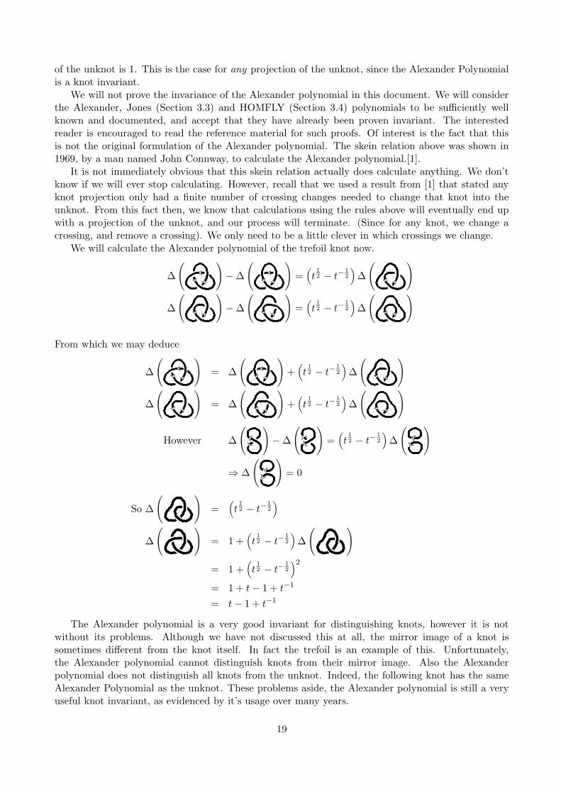
of the unknot is 1. This is the case for any projection of the unknot, since the Alexander Polynomialis a knot invariant.

We will not prove the invariance of the Alexander polynomial in this document. We will considerthe Alexander, Jones (Section 3.3) and HOMFLY (Section 3.4) polynomials to be sufficiently wellknown and documented, and accept that they have already been proven invariant. The interestedreader is encouraged to read the reference material for such proofs. Of interest is the fact that thisis not the original formulation of the Alexander polynomial. The skein relation above was shown in1969, by a man named John Connway, to calculate the Alexander polynomial.[1].

It is not immediately obvious that this skein relation actually does calculate anything. We don’tknow if we will ever stop calculating. However, recall that we used a result from [1] that stated anyknot projection only had a finite number of crossing changes needed to change that knot into theunknot. From this fact then, we know that calculations using the rules above will eventually end upwith a projection of the unknot, and our process will terminate. (Since for any knot, we change acrossing, and remove a crossing). We only need to be a little clever in which crossings we change.

We will calculate the Alexander polynomial of the trefoil knot now.

∆

( )−∆

( )=(t

12 − t− 1

2

)∆

( )

∆

( )−∆

( )=(t

12 − t− 1

2

)∆

( )

From which we may deduce

∆

( )= ∆

( )+(t

12 − t− 1

2

)∆

( )

∆

( )= ∆

( )+(t

12 − t− 1

2

)∆

( )

However ∆

( )−∆

( )=(t

12 − t− 1

2

)∆

( )

⇒ ∆

( )= 0

So ∆

( )=

(t

12 − t− 1

2

)

∆

( )= 1 +

(t

12 − t− 1

2

)∆

( )

= 1 +(t

12 − t− 1

2

)2

= 1 + t− 1 + t−1

= t− 1 + t−1

The Alexander polynomial is a very good invariant for distinguishing knots, however it is notwithout its problems. Although we have not discussed this at all, the mirror image of a knot issometimes different from the knot itself. In fact the trefoil is an example of this. Unfortunately,the Alexander polynomial cannot distinguish knots from their mirror image. Also the Alexanderpolynomial does not distinguish all knots from the unknot. Indeed, the following knot has the sameAlexander Polynomial as the unknot. These problems aside, the Alexander polynomial is still a veryuseful knot invariant, as evidenced by it’s usage over many years.

19

3.3 The Jones Polynomial

The Jones polynomial is named after it’s creator, Vaughn Jones from New Zealand. He discoveredthis invariant in 1984 whilst working on operator algebras, something completely unrelated (at leastat the time) to knot theory.

The Jones polynomial, denoted VK for a knot K, is simply the Kauffman Polynomial X with thesubstitution A = t−

14 into the X polynomial. That’s it. Really. It is clearly an invariant, since it is

the same invariant as the X polynomial which we put so much work into showing invariance for.Since we have been working with the trefoil so much in this section, we will continue doing so now

by calculating it’s Jones polynomial.

V =(t−

14

)−4+(t−

14

)−12−(t−

14

)−16= t+ t3 − t4

This is not the usual way of coming by the Jones polynomial, however. The Jones polynomial isusually arrived at by a set of rules that includes a skein relation like that of the Alexander polynomial.Those rules are:

V = 1 (6)

t−1VL+ − tVL− =(t

12 − t(− 1

2))VL0 (7)

Since we know that the Jones polynomial is an invariant, we know that (6) applies to any projectionof the unknot. The second rule (7), is a skein relation that describes a relation between the Jonespolynomial of any three almost identical projections that differ only at one crossing according toFigure 23 above.

The Jones polynomial is capable of distinguishing more knots than the Alexander polynomial. Inparticular it can distinguish all knots of nine crossings or less. The first pair of knots that it cannotdistinguish are an eight crossing prime knot and a ten crossing prime knot [6]. These knots are shownbelow in Figure 24. It is clear then that the Jones polynomial is not a complete invariant. What is

Figure 24: These two knots have the same Jones polynomial

unclear is whether or not the Jones polynomial is capable of distinguishing the unknot from everyother knot. This would be a very useful attribute to have in a knot invariant, but remains an openquestion.

3.4 The HOMFLY Polynomial

The HOMFLY Polynomial came about four months after Vaughn Jones discovered the Jones Poly-nomial. The name HOMFLY is derived from the names of those who discovered it; Hoste, Ocneau,Millett, Freyd, Lickorish and Yetter. The polynomial itself, is a Laurent polynomial in two variables(α, z). We denote the HOMFLY polynomial of a link L to be P (L)

20

To calculate the HOMFLY polynomial, another skein relation is used. The rules look very similarto those of the Alexander polynomial, and of the skein relationship we showed for the Jones polynomial.This is no accident, the creation of the HOMFLY was a direct result of attempts to generalise theAlexander and Jones polynomials. We will show later that the Alexander and Jones polynomials areboth special cases of the HOMFLY polynomial.

To calculate the HOMFLY polynomial, the following rules are used:

P ( ) = 1 (8)

αP (L+)− α−1P (L−) = zP (L0) (9)

where (8) holds for any projection of the unknot, and L+, L−, L0 are three identical links differingonly by one crossing as with the other skein relations and Figure 23.

We have already stated that the HOMFLY polynomial is a generalisation of both the Alexanderand Jones polynomials. Let us examine this a little more closely. Look at (9). If we let α = t−1 and

z = t12 − t(− 1

2) then our equation becomes

t−1P (L+)− tP (L−) =(t

12 − t(− 1

2))P (L0)

which is the skein relation for the Jones polynomial. Also if we let α = 1 and z = t12 − t(− 1

2) then the

equation becomes

P (L+)− P (L−) =(t

12 − t(− 1

2))P (L0)

which is the skein relation for the Alexander polynomial.Let us calculate the HOMFLY polynomial of the trefoil knot. The skein relation tells us that

αP

( )− α−1P

( )= zP

( )

αP

( )− α−1P

( )= zP

( )

From which we may deduce

P

( )= α−1

(α−1P

( )+ zP

( ))

= α−2 + α−1zP

( )

P

( )= α−1

(α−1P

( )+ zP

( ))

= α−2P

( )+ α−1z

However αP

( )− α−1P

( )= zP

( )

⇒ P

( )= z−1

(α− α−1

)

So P

( )= α−2P

( )+ α−1z

21

= α−2(z−1α− z−1α−1

)+ α−1z

= z−1α−1 − z−1α−3 + α−1z

P

( )= α−2 + α−1zP

( )

= α−2 + α−1z(z−1α−1 − z−1α−3 + α−1z

)

= α−2 + α−2 − α−4 + α−2z2

= 2α−2 − α−4 + α−2z2

Now if we substitute in α = t−1 and z = t12 − t(− 1

2)

V = 2(t−1)−2−(t−1)−4

+(t−1)−2 (

t12 − t(− 1

2))2

= 2t2 − t4 + t2(t− 2 + t−1

)

= 2t2 − t4 + t3 − 2t2 + t

= t+ t3 − t4

Which is exactly the polynomial we calculated for the Jones polynomial of the trefoil, above. We mayalso substitute α = 1 and z = t

12 − t(− 1

2) in order to calculate the Alexander polynomial of the trefoil.

∆

( )= 2 · 1−2 − 1−4 + 1−2

(t

12 − t(− 1

2))2

= 1 + (t− 2 + t−1)

= t− 1 + t−1

The HOMFLY polynomial is the most powerful yet of all the polynomial invariants. It is notcomplete, however, [1] shows two knots that have the same HOMFLY polynomial. The HOMFLYpolynomial also has some interesting properties. For two knots J and K, the following hold thecomposition of the two knots has HOMFLY polynomial P (J#K) = P (J)P (K) which is the productof the polynomials of the factor knots. Also the splittable link of J and K has HOMFLY polynomialP (J ∪K) = z−1

(α− α−1

)P (J)P (K). We saw a particular case of this above with the trivial link of

two components when we were calculating the HOMFLY polynomial for the trefoil knot.

4 Concluding Remarks

We have really only scratched the surface of knot theory in this document. There is much we havenot discussed such as types of knots , notations for describing knots, braids, the list goes on. We havenot dealt with the topological significance of knots, nor have we discussed knots in dimensions higherthan three. The interested reader is encouraged to persue any and all of these topics, and any otherrelated topics as well.

What we have discussed is a good introduction to the concepts and definitions involved with knottheory and, motivated by the desire to be able to distinguish different knots, we have discussed andexamined the idea of knot invariants. We have by no means exhausted the list of invariants, althoughwe have looked at most of the “big players” of the knot invariants. The following two open questions,and many others remain.

• Do the Jones or HOMFLY polynomials distinguish the unknot from all other knots?

• Find a complete knot invariant.

One can find many other open problems in [1] as well as [10].The reader is now encouraged, armed with the information discussed in these pages, to continue

their study of knots through the reference material or any other reference material at their disposal.

22

References

[1] Colin C. Adams: The Knot Book - An Elementary Introduction to the Mathematical Theory ofKnots. W. H. Freeman and Company. New York, 1994

[2] John L. Casti: Five More Golden Rules - Knots, Codes, Chaos and Other Great Theories of20th-Century Mathematics. John Wiley & Sons, Inc, 2000

[3] Arun Ram: Quantum Groups. at the Workshop on Algebra, Geometry, and Topology 22 Januaryto 9 February Australian National University Canbera, 1996

[4] V.F.R. Jones: Milnor’s Work and Knot Polynomials. From Topological Methods in ModernMathematics (Stony Brook, New York, 1992) pp195-202

[5] Vaughan F. R. Jones: Von Neumann Algebras in Mathematics and Physics. A plenary addresspresented at the International Congress of Mathematicians held in Kyoto, August 1990.

[6] Vaughan F. R. Jones: Subfactors and Knots. American Mathematical Society. Providence, RhodeIsland, 1991

[7] J. Scott Carter How Surfaces Intersect in Space - An introduction to topology. World Scientific.second edition. 1995

[8] Michael Atiyah The geometry of Physics and Knots. Cambridge University Press. 1998

[9] Eric Weisstein’s World of Mathematics. A free service for the mathematical community providedby Wolfram Research, makers of Mathematica, with additional support from the National ScienceFoundation. http://mathworld.wolfram.com/

[10] A List of Approachable Open Problems in Knot Theory.http://www.williams.edu/Mathematics/cadams/knotproblems.html

23