an introduction to drip irrigation system
TRANSCRIPT


AN INTRODUCTIONTO
DRIP IRRIGATION SYSTEMS
NEW DELHI PUBLISHERSNew Delhi
Ajai SinghAssistant Professor in Soil and Water Conservation
Uttar Banga Krishi ViswavidyalayaWest Bengal

© Publishers
First Edition 2012
ISBN: 978-93-81274 -18-7
All rights reserved. No part of this book may be reproducedstored in a retrieval system or transmitted, by any means, electronic
mechanical, photocopying, recording, or otherwisewithout written permission from the publisher
New Delhi Publishers90, Sainik Vihar, Mohan Garden, New Delhi – 110 059
Tel: 011-25372232, [email protected]/gmail.com
Website: www.ndpublisher.in
Ajai Singh, An Introduction to Drip Irrigation Systems, New Delhi Publishers,New Delhi

Dedicated toMy Mother-in-Law
LALALALALATE SMTTE SMTTE SMTTE SMTTE SMT. SHANTI DEVI. SHANTI DEVI. SHANTI DEVI. SHANTI DEVI. SHANTI DEVI

CHAPTER 1

Foreword
Water is a natural resource which can not be replenished. As the demandfor water is growing up from all the user groups, lesser water will beavailable for agriculture. Efficient water use is necessary for sustainablecrop production and drip irrigation proved to provide efficiently irrigationwater and nutrients to the roots of plants, while maintaining high yieldproduction. Since not all the soil surface is wetted under irrigation, lesswater is required for irrigation. Modern drip irrigation has become themost valued innovation in agriculture. Higher water application efficienciesare achieved with drip irrigation due to reduced soil evaporation, less surfacerunoff and minimum deep percolation.
The knowledge about drip system and its design principles is essential forthe students of Agricultural Engineering and professionals of WaterResources Engineering. I am sure that this book, which includes the basicsof drip system and recent published research work on designing of dripirrigation system, will serve the student community as well as Faculties ofAgricultural Engineering Department to a great extent by providing up todate information in a clear and concise manner.
I would like to compliment Dr. Ajai Singh for having brought out thistextbook with quite useful and valuable information for the AgriculturalEngineering Under Graduate and Post Graduate students in India.
Prof. (Dr.) Sabita Senapati Director of Research
Uttar Banga Krishi Viswavidyalaya Coochbehar, West Bengal, India


Preface
Excessive and improper use of water due to lack of information has becomea common practice to grow more water intensive crops and earn more. Thewater resources are being depleted by current practice of farming and wewill be devoid of sufficient irrigation water if the trend continues in theyears to come. Time has come now to focus on judicious and efficient useof water for agricultural purpose. Adoption of Micro Irrigation System canbe a panacea in irrigation related problems. In this technology, the croppedfield is irrigated in the close vicinity of root zone of crop. It reduces thewater loss occurring through evaporation, conveyance and distribution.Therefore high water use efficiency can be achieved. The unirrigated rainfedcropped area can be increased with this technology and potential source offood production for the benefit of country’s food security could beaugmented. The Government of India has been considering rapid promotionof use of plastics in agriculture and micro irrigation as a major step inimproving overall horticultural crop yields and water use efficiency. Themicro irrigation has gained considerable growth in the country due tofinancial assistance provided by the centrally sponsored subsidy scheme.This book is designed as a professional reference book with basic andupdated information and its aim is to meet the needs of students ofagricultural engineering under graduate and post graduate degree program.The practicing engineers, agricultural scientists working in the field ofagricultural water management and officers of Agriculture and HorticultureDepartments of State Government will find this book useful. In this book,the basics of drip irrigation, types, components, design, installation,operation and maintenance are presented. Efforts have been made toincorporate the recent published works in peer reviewed journals atappropriate place. An additional chapter on automation of micro irrigationsystem has also been included. Numerical problems and examples have

(viii)
been added to emphasize the design principles and make the understandingof the subject matter.
I owe my deepest gratitude to Dr. A. K. Das, Vice–Chancellor, UBKV, Dr.S. K. Senapati, Director of Research, UBKV, Dr. Goutam Mondal, Incharge,RRS, Majhian, and all my colleagues and other staff of Regional ResearchStation, Majhian, for their best wishes and constant encouragement. Theauthor is grateful to many individuals and organizations for the assistanceprovided at different stages of preparation of manuscript and supply of usefulliterature. I sincerely thank Dr. K. N. Tiwari, Professor, Agricultural &Food Engineering Department, IIT, Kharagpur, under whom I worked in aPlasticulture Development Centre Project, for his blessings and affection.I am heartily thankful to Prof. (Dr.) Mohd. Imtiyaz, Prof. (Dr.)R. K. Isaac, Prof. (Dr.) D. M. Denis, Dr. Arpan Shering, Associate Professor,Dr. S. K. Srivastava, Assistant Professor of Department of Soil, Land andWater Engineering and Management, Vaugh School of AgriculturalEngineering & Technology, Sam Higginbottom Institute of Agriculture,Technology & Sciences, Allahabad for continuous encouragement andsupport. I am grateful to Dr. R. P. Singh, Professor, Irrigation and DrainageEngineering Department, GBPUAT, Pantnagar for his kind blessing andencouragement. The author is indebted to many people and institution/organizations for providing the material and issuing the permission undercopyright act for inclusion in this textbook. I wish to acknowledge the supportreceived from the Food and Agricultural Organisation, Arizona CooperativeExtension, Arizona State University and Dr. Richard John Stirzaker ofCSIRO, Division of Land and Water, Australia for providing the figures andtechnical details. The author has tried to acknowledge the every source ofinformation, any omission is inadvertent. This can be pointed out and will beincluded in the book at appropriate time.
I feel profound privilege in expressing my heartfelt reverence to my parents,brothers and sister, in-laws for their blessings and moral support to achievethis goal. Last but not the least I acknowledge with heartfelt indebtness,the patience and the generous support rendered by my better half, Punamand daughter Anushka who always allowed me to work continuously withsmile on their face. I offer my regards and blessings to all of those whosupported me in any respect during the completion of this book. Authorwould welcome suggestions from readers to improve the text of book.
Dr. Ajai Singh([email protected])

Contents
Foreword vPreface vii
1. Introduction 1
2. Drip Irrigation Systems 52.1 Types of Micro Irrigation System 62.1.1 Drip irrigation 62.1.2. Sub-surface system 62.1.3. Bubbler 82.1.4. Micro-sprinkler 82.1.5. Pulse system 102.2. Advantages of Drip Irrigation 102.3. Problems and Demerits of Drip Irrigation 112.4 Suitability of Drip Irrigation 112.4.1. Crops 112.4.2. Slopes 112.4.3. Soils 112.4.4. Irrigation Water 122.5. Quantitative Approach of Wetting Patterns 12
3. Components of Drip Irrigation Systems 253.1. Control Head 253.1.1. Pump/Overhead Tank 253.1.2. Fertigation 283.1.2.1. Advantages 293.1.2.2. Limitations and Precautions 293.1.2.3. Fertigation methods 303.1.2.4. Fertigation Recommendations 333.1.2.5. Plant Nutrients 373.1.2.6. Sources of Fertilizers 413.1.2.7. Nutrient Monitoring 423.1.3. Filtration System 43

(x)
3.1.3.1. Selection of Filters 443.1.3.2. Types of Filters 443.1.3.3. Filter Characteristics and Evaluation 503.2. Distribution Network 503.2.1. Main and Sub-main Line 513.2.2. Laterals 513.2.3. Drippers/Emitters 513.2.3.1. Types of Drippers/Emitters 533.2.3.2. Emitter Discharge Exponent 553.2.3.3. Selection of an Emission Device 553.2.3.4. Emitter Spacing 57
4. Estimation of Crop Water Requirement 594.1. Methods of Evapotranspiration Estimation 604.1.1. Direct Methods of Measurement of Evapotranspiration 604.1.1.1. Pan Evaporation Method 604.1.1.2. Soil Moisture Depletion Method 674.1.2. Empirical Methods 684.1.2.1. Thornthwaite Method 684.1.2.2. Blaney – Criddle Method 694.1.2.3. Hargreaves Method 704.1.3. Micrometeorological Method 704.1.3.1. Mass Transport Approach 704.1.3.2. Aerodynamic Approach 734.1.4. Energy Balance Approach - Bowen ratio Method 744.1.5. Combination Methods 764.1.5.1. Penman Method 764.1.5.2. Modified Penman Approach 804.1.5.3. Van Bavel Method 834.1.5.4. Slatyer and Mcllroy Method 834.1.5.5. Priestley and Taylor Method 854.1.6. Methods in Remote Sensing Technology 864.2. Crop Water Requirement in Greenhouse Environments 874.3. Computer Models to Estimate Evapotranspiration 894.3.1. ETo Calculator 894.3.2. Cropwat 894.4. Computation of Crop Water Requirement with Limited Wetting 90
5. Irrigation Scheduling 935.1. Advantages of Lrrigation Scheduling 945.2. Methods of Irrigation Scheduling 94

(xi)
5.2.1. Water Balance Approach 945.2.2. Soil Moisture Measurement 975.2.2.1. Neutron Probe 995.2.2.2. Electrical Resistance 1015.2.2.3. Soil Tension 1035.2.2.4. Time-Domain Reflectometry (TDR) 1035.2.2.5. Frequency-Domain Reflectometers (FDR) 1055.2.2.6. Infrared/Canopy Temperature 1065.2.3. Wetting Front Detector 107
6. Hydraulics of Water Flow in Pipes 1116.1. Flow in a Pipe 1116.2. Water Pressure 1136.3. Estimation of Total Head 1146.4. Head loss due to Friction in Plain Pipes 1156.4.1. Hazen-William’s Formula 1156.4.2. Darcy- Weisbach’s Formula 1166.4.3. Watters and KellerFormula 1176.5. Head loss Fue to Friction in Multi-outlet Pipes 118
7. Planning and Design of Drip Irrigation Systems 1237.1. Collection of General Information 1247.2. Layout of the Drip Irrigation System 1247.3. Crop Water Requirement 1247.4. Hydraulic Design of Drip Irrigation System 1257.4.1. Development in Design of Lateral pipe 1267.4.1.1. Hydraulic Analysis of Laterals 1287.4.2. Design of Sub-main 1447.4.3. Design of Main 1447.5. Pump Horse Power Requirement 1457.6. Design Tips for Drip Irrigation 1597.7. Economic Analysis 1607.7.1. Depreciation 1617.7.2. Escalation Cost 1627.7.3. Capital Recovery Factor 1627.7.4. Discounting Methodology 1637.7.4.1. Net Present Value (NPV) 1637.7.4.2. Benefit Cost Ratio (BCR) 1647.7.4.3. Internal Rate of Return (IRR) 164

(xii)
8. Performance Evaluation of Emission Devices 1738.1. Manufacturing Characteristics 1738.1.2. Mean Flow Rate Variation 1748.2. Hydraulic Characteristics 1758.3. Operational Characteristics 1768.3.1. Emission Uniformity 1768.3.2. Absolute Emission Uniformity 1768.3.3. Emission Uniformity 1778.3.4. Uniformity Coefficient 1778.4. Water Application Uniformity - Statistical Uniformity 178
9. Installation, Management and Maintenance of Drip IrrigationSystems 181
9.1. Installation 1819.1.1. Installation of Filter Unit 1819.1.2. Installation of Mains and Sub-mains 1829.1.3. Laying of Laterals 1829.2. Testing of the System 1829.3. Maintenance of Drip Irrigation System 1839.3.1 Flushing the Mainline, Sub-main and Laterals 1849.3.2. Filter Cleaning 1849.3.2.1. Media Filter 1859.3.2.2. Screen Filter 1859.3.3. Chemical Treatment 1859.3.3.1. Acid Treatment 1869.3.3.2. Chlorine Treatment 186
10. Salt Movement Under Drip Irrigation Systems 18910.1. Salinity Measurement 19210.2. Leaching Requirements 19310.3. Salt tolerance of the Crop and Yield 19510.4. SALTMED Model 19710.4.1. Equations of the Model 198
11. Automation of Drip Irrigation Systems 20311.1 Types of Automation 20411.1.1. Hydraulically Operated Sequential System 20411.1.2. Volume Based Sequential Hydraulically Automated
Irrigation System 20611.1.3. Time Based Electrically Operated Sequential System 207

(xiii)
11.1.4. Non-sequential Systems 20711.1.4.1. Feedback Control System 20811.1.4.2. Inferential Control System 20911.2. Components of Automated Irrigation System 20911.2.1. Irrigation Controllers 20911.2.2. Soil Moisture Sensors 209References 212Appendix 219Index 227


1Introduction
India is predominantly an agricultural country and 15 percent of totalexport and 65% of total population’s livelihood are supported byagriculture. Agriculture contributes 30% of total gross domestic productof the country. After independence, we have made remarkable progressin achieving food security in a sustainable manner. Land and Waterare two most important resources for any activity in the field ofagriculture. Water is such a natural resource which can not bereplenished and its demand is increasing alarmingly. The country isendowed with many perennial and seasonal rivers. The river systemwhich constitutes 71 per cent of water resources is concentrated in 36% of geographic area. Most of agricultural fields are irrigated by useof underground water for assured irrigation. Rainfall is a source forwater for rainfed agriculture. In present times, the water resourcesplay a very significant role in development and constitute a criticalinput for economic planning in developing countries. Large investmentsand phenomenal growth in the irrigation sector, the returns fromirrigated systems in terms of crop yield, farm income and cost recoveryare disappointing. Apart from that, there are additional problems ofincrease in soil salinity, water logging and social inequity. There is alarge gap between the development and utilization of irrigation potentialcreated. If we go back to the past of development of drip irrigationsystem, we find that Davis (1974) used subsurface clay pipes withirrigation and drainage systems in an experiment. Irrigation of plantsthrough narrow openings in pipes can also be traced back to green

2 AN INTRODUCTION TO DRIP IRRIGATION SYSTEM
house operations in the United Kingdom in the late 1940s (Davis,1974). Blass (1964) observed that a tree near a leaking faucet exhibiteda more vigorous growth than other trees in the area. He worked on itand developed the current form of drip irrigation technology and gotpatented. The availability of low cost plastic pipe for water deliverylines was one of the reasons which helped to spread the application ofdrip irrigation systems. Gradually the area under drip irrigationincreased throughout the world especially in countries where waterwas a scarce resource. INCID (2009) reported that area covered underdrip system was 0.41 Mha in 1981 which increased to 8.0 Mha in2009. Although drip irrigation systems are considered the leading watersaving technologies in irrigated agriculture, their adoption is still low.At present, of the total world irrigated area, about 2.9% (8 million ha)is equipped with drip irrigation. Most of the drip irrigated area isconcentrated in Europe and the America. Asia has the highest areaunder irrigation (193 million ha, which is 69% of the total irrigatedarea), but has very low area of 1.8 million ha (<1.0%) under dripirrigation. In some countries such as Israel & Jordan, where wateravailability limits crop production, drip irrigation systems irrigate about75% of the total irrigated area. In India it accounts for 2.3% of thetotal irrigated area (62.3 million ha). While the ultimate potential fordrip irrigation in India is estimated at 27 million ha. Drip irrigation,like other irrigation methods, will not fit every agricultural crop, specificsite or objective. Presently, drip irrigation has the greatest potentialwhere (i) water and labor are expensive or scarce; (ii) water is ofmarginal quality viz., saline; (iii) soils are sandy, rocky or difficult tolevel, (iv) steep slopes and undulated topography; and (v) high valuecrops are produced. The principal crops under drip irrigation arecommercial field crops (sugarcane, cotton, tobacco etc), horticulturalcrops – fruit & orchard crops, vegetables, flowers, spices & condiments,bulb & tuber crops, plantation crops and silviculture/forestryplantations. This method of irrigation continues to be important in theprotected agriculture viz., greenhouses, shade nets, shallow & walkingtunnels etc., for production of vegetables & flowers. Drip irrigation isalso used for landscapes, parks, highways, commercial developmentsand residences. Undoubtedly, the area under drip irrigation will continue
INTRODUCTIN 3
to increase rapidly as the amount of water available to agriculturedeclines and the demands for urban and industrial use increase. Dripirrigation is also one of the techniques that enable growers to overcomesalinity problems that currently affect 8.0 million ha area in India. Asthis area increases, so too will the use of Drip irrigation to maintaincrop production. In addition, because growers are looking to reducecost of production but at the same time improve crop quality, theimproved efficiency provided from drip irrigation technology willbecome increasingly important.
Apart from drip irrigation systems or we can say micro-irrigationsystems; there are several indigenous low pressure low volumeirrigation systems. For example, there are Pitcher methods, low costdrip irrigation systems and bamboo based drip irrigation systems. Underpitcher methods, earthen pots with a hole on the bottom are placed in aring basin made around the plants. Pots can be of 10-20 liter capacityand need to be refilled when gets empty. Pitcher method is used forirrigation of small area and where energy availability is irregular. Asimple low-cost drip irrigation system uses plastic pipes laid on thesurface to irrigate vegetables, field crops and orchards. Water isdelivered through the small holes made in the hose. It can consist of a20 liter bucket with 30m of hose or drip tape connected to the bottomof the tank. The bucket is placed at 1-2m above the ground so thatgravitation head can create sufficient water pressure to ensure wateringof the crops. Maintenance usually involves repairing the leakages inthe pipes and joints and clearing blockages. Bamboo drip irrigationmethod is used to divert the part of the flow of hillside stream by usinga hallow bamboo in place of earthen channel. Govt. of India is alsoproviding subsidy to farmers in order to boost up the adoption of thisdrip irrigation technology among the farmers. Drip irrigation techniqueshas always been considered to be adopted only in water scarce areabut I strongly believe that time has come to adopt and propagate thissystem in areas endowed with abundant supply of water just to makesure the sustainable development of agriculture.


2Drip Irrigation Systems
Micro irrigation is defined as slow application of water above or belowthe soil surface near the vicinity of plant roots. Water is applied in theform of drops, sprayed over the land surface or in small continuousstream through fixed applicator near the plants. The basic conceptunderlying the micro irrigation method is to supply the amount of waterneeded by the plant within a limited volume of the soil rather thanwetting the whole area. Micro-irrigation refers to low-pressureirrigation systems that spray, mist, sprinkle or drip. Water is appliedclose to plants so that only part of the soil in which the roots grown iswetted, unlike surface and sprinkler irrigation, which involves wettingthe whole soil profile. In this method of irrigation, a dense root systemis developed in the zone adjacent to the dripper, resulting in direct andtherefore more efficient water use by the plant. A network of pipes anda large number of drippers are required in the field because the dischargeof a dripper is small (2 to 8 lph). With micro irrigation, waterapplications are more frequent than with other methods and thisprovides a very favorable moisture level in the soil in which plantscan flourish. This system is best suited to the area having scanty rainfallor poor quality irrigation water is being used. The low volume irrigationsystems are also suitable for almost all orchards crops, plantation cropsand most of the vegetable crops. Micro-irrigation has gained attentionduring recent years because of its potential to increase yields anddecrease water, fertilizer, and labor requirements if managed properly.

6 AN INTRODUCTION TO DRIP IRRIGATION SYSTEM
2.1 Types of Micro Irrigation System
The micro irrigation system is classified based on the installation method,emitter flow rate, wetted soil surface area or the mode of operation.Types of the micro irrigation systems are briefly described below.
2.1.1 Drip Irrigation
Drip irrigation applies water directly to the soil surface and allows thewater to dissipate under low pressure in a form of drops. A wettedprofile develops in the plant’s root zone beneath each dripper. Theshape depends on soil characteristics, but often it is onion-shaped.Ideally, the area between rows or individual plants remains dry andreceives moisture only from incidental rainfall. In this system, theemitters and laterals are laid on the land surface. It has been primarilyused on widely spaced plants, but can also be used for row crops.Generally, discharge rates are less than 12 lph for single outlet point-source emitter and less than 12 lph per meter of lateral for line-sourceemitters. Advantages of this system include the ease of installation,changing and cleaning the emitters and measuring individual emitterdischarge. Often the terms drip and trickle irrigation are consideredsynonymous. It is suitable for establishing the forestry plantations underwasteland development program. Still we are applying drip irrigationto water scarce area to grow the crops.
2.1.2. Sub-surface System
It is a system in which water is applied slowly below the surface throughthe line-source emitters. The water is applied through emitters withdischarge rate generally in the range of 0.6 to 4 lph. A thin walled dripline has internal emitters glued together at pre-defined spacings withina thin plastic distribution line. The drip line is available in a widerange of diameters, wall thickness, emitter spacing, and flow rates.The emitter spacing is selected to closely fit plant spacing for mostrow crops. Drip lines are buried below the ground and therefore calledsub-surface drip irrigation systems. Burial of the drip line is preferableto avoid degradation from heat, ultraviolet rays and displacement fromstrong winds. These systems are used on small fruits and vegetablecrops. Advantages of subsurface system include freedom from

DRIP IRRIGATION SYSTEMS 7
Fig. 2.1: Emitter connected with the lateral (Jain Irrigation Systems)
Fig. 2.2.: Sub-surface drip irrigation systems (source: Peter Thorburn,www.askgillevy.com)

8 AN INTRODUCTION TO DRIP IRRIGATION SYSTEM
anchoring of the lateral lines at the beginning and removing them atthe end of the growing season, little interference with cultivation andpossibly a longer operational life.
2.1.3. Bubbler
Bubblers are very similar to the point source on-line emitters in shapebut differ in performance. In this system, the water is applied to thesoil surface in a small stream or fountain from an opening with a point-source. The discharge rate is usually greater than surface or subsurfacedrip irrigation but usually less than 225 lph. A small basin is requiredto control the distribution of water. Advantages of bubbler system arereduced filtration, maintenance or repair and energy requirements ascompared with other micro irrigation systems. Larger size lateral isused with this system to reduce the pressure loss associated with ahigh discharge rate. The bubbler heads are used in planter boxes, treewells, or specialized landscape applications where deep localizedwatering is preferable. High irrigation application efficiency up to 75%can be achieved with total control of the irrigation water. Anotheradvantage is that the entire piping network is buried, so there are noproblems in field operations. Associated disadvantages are notsupplying the small water flows as in other micro-irrigation systems.It is not possible to achieve a uniform water distribution over the treebasins in sandy soils with high infiltration rates.
2.1.4. Micro-sprinkler
This is a combination of sprinkler and drip irrigation. Water is sprinkledaround the root zone of plants with a small sprinkler working underlow pressure. Water is given only to the root zone area as is in the caseof drip irrigation but not to the entire ground surface as done in thecase of sprinkler irrigation method. Depending on the water throwpatterns, the micro-sprinklers are referred to as mini-sprays, micro-sprays, jets, or spinners. The sprinkler heads are external emittersindividually connected to the lateral pipe typically using spaghettitubing, which is very small (1/8 inch to 1/4 inch) diameter tubing. Thesprinkler heads can be mounted on a support stake or connected to thesupply pipe. Micro-sprinklers are desirable because fewer sprinkler

DRIP IRRIGATION SYSTEMS 9
Fig. 2.3: Bubbler placed near the tree and fitted with underground pipelines
Fig. 2.4.: Micro-sprinkler spraying the water(source:www.agricultureinformation.com)

10 AN INTRODUCTION TO DRIP IRRIGATION SYSTEM
heads are necessary to cover larger areas. Micro sprinklers require 35kPa to 300 kPa of pressure for operation. Discharge rates usually varyfrom 15 lph to 200 lph. Micro sprinkler system is less likely to clogthan a drip irrigation system, but water losses due to wind drift andevaporation are greater.
2.1.5. Pulse System
Pulse system uses high flow rate emitters and consequently has a shorterwater application time. Pulse systems have application cycles of 5,10, or 15 minutes in an hour, and flow rates for pulse emitters are 4 to10 times larger than the conventional surface drip irrigation system.The primary advantage of this system is a possible reduction in theclogging problems.
2.2. Advantages of Drip Irrigation
The main advantages of drip irrigation system are:
• Water saving
• Enhanced plant growth and yield
• Uniform and better quality of produce
• Efficient and economic use of fertilizers
• Less weed growth
• Possibility of using saline water
• Energy saving
• Can be automated
• Improved production on undulating land conditions
• No soil erosion
• Flexibility in operation
• Labor saving
• No land preparation
• Minimum disease and pest infestation

DRIP IRRIGATION SYSTEMS 11
2.3 Problems and Demerits of Drip Irrigation
The demerits and problems of drip irrigation system are given below:
••••• Clogging of drip emitters by particulate, chemicals and biologicalmaterials.
••••• Shallow root development is limited to the wetted portion ofroot zone, resulting reduced ability of trees to withstand againsthigh winds.
••••• Persistent maintenance requirement
••••• Salinity hazards
••••• Technical skill is required for design and installation
2.4 Suitability of Drip Irrigation
Drip irrigation systems can be adopted under the following conditions:
2.4.1. Crops
Drip irrigation is most suitable for vegetables, fruits, sugarcane, andcereal crops except paddy. The high value crops such as fruit cropsgive early recovery of capital investment on installation of a microirrigation system. These systems are also suitable for plantation cropssuch as coconut, coffee, cardamom, cumin, citrus, grapes and mango.Close growing crops will require more investment, otherwise for widelyspaced crops, these systems can be easily installed.
2.4.2. Slopes
Drip irrigation is adaptable to any cultivable slope. Normally the cropsand laterals are planted along contour lines. This practice minimizesthe change in emitter discharge due to change in land elevations.
2.4.3. Soils
Drip irrigation is suitable for most of the soils. For example, on claysoils, irrigation water should be applied slowly to avoid ponding andrunoff. On sandy soils, higher emitter discharge will be appropriate toensure lateral movement of the water into the soil. It can be applied to

12 AN INTRODUCTION TO DRIP IRRIGATION SYSTEM
irrigate crops grown on undulating land topography and slopes wherethe depth of soil is limited.
2.4.4. Irrigation Water
One of the major problems with drip irrigation is emitters clogging.All emitters have very small openings ranging from 0.2-2.0 mm indiameter and these can be clogged with the use of dirty water. Thus, itis essential to install filters for irrigation water to be free fromsediments. Micro sprinklers can eliminate problem of clogging to acertain extent. Clogging may also occur if the water contains algae,fertilizer deposits and dissolved chemicals which precipitate such ascalcium and iron. Filtration may remove some of the materials. Dripirrigation is also suitable for poor quality water (saline water).Supplying water to individual plants also means that the method canbe efficient to increase the water use efficiency and thus most suitablewhere water is scarce resources.
2.5. Quantitative Approach of Wetting Patterns
Due to the manner in which water is applied by a drip irrigation system,only a portion of the soil surface and root zone of the total field iswetted unlike surface and sprinkler irrigation systems. Water flowingfrom the emitter is distributed in the soil by gravity and capillary forcescreating the contour lines similar to onion shape. The exact shape ofthe wetted volume and moisture distribution will depend on the soiltexture, initial soil moisture, and to some degree, on the rate of waterapplication. Figs. 2.5 & 2.6 show the effects of changes in dischargeon two different soil types, namely sand and clay. The water savingsthat can be made using drip irrigation are the reductions in deeppercolation, surface runoff and evaporation from the soil. It is evidentfrom the Fig.2.7 that soil moisture content in the soil always remainsat or around the field capacity in drip irrigation, where as in sprinklerand surface irrigation methods, crops face over irrigation and waterstress during certain period. In the line source type of drip irrigationsystem where the emitters are spaced very closely, individual onionpatterns creates a continuous moisture zone. The knowledge about thewetting patterns under emitters is essential in selecting the appropriate

DRIP IRRIGATION SYSTEMS 13
Fig. 2.5: Wetting patterns for sandy soils with high and low discharge rates emitters
Fig. 2.6: Wetting patterns for clay soils with high and low discharge rates emitters

14A
N IN
TR
OD
UC
TIO
N T
O D
RIP IR
RIG
AT
ION
SYST
EM
Fig. 2.7: Moisture availability for crops in different irrigation methods

DRIP IRRIGATION SYSTEMS 15
spacing of the emitters. Distance between emitters and emitter flowrates must match to the wetting characteristics of the soil and the amountand timing of water to be supplied to meet the crop needs.
Under drip irrigation, the ponding zone that develops around the emitteris strongly related to both the application rate and the soil properties.The water application rate is one of the factors which determine thesoil moisture regime around the emitter and the related root distributionand plant water uptake patterns. Drip irrigation systems generallyconsist of emitters that have discharge varying from 2.0 to 8.0 lph. Insemi-arid climates, crop water use during the summer can be 6 to 8mm/d with water supplied two or three times a week. When the waterapplication exactly equal to the plant water need, then also, part of thewater may not be used by the plant and it would most likely leachbelow the root zone. Therefore, lowering the emitter discharge to asclose as possible to the plant water uptake rate can improve irrigationefficiency. Recently, microdrip irrigation systems have been developedthat provide emitter discharges of 0.5 lph. These systems have beenstudied most intensively in greenhouses (Koenig, 1997), andpreliminary results showed that they reduced water consumption oftomato plant by 38%, increased yield by 14 to 26%, and reducedleaching fraction by 10 to 40%. In a recent application on sweet cornunder field conditions, Assouline et al. (2002) have shown thatmicrodrip irrigation may improve yield, reduce drainage flux, and affectthe water content distribution within the root zone, especially throughan increased drying of the 0.60 to 0.90m soil layer compared withconventional drip irrigation.
The microdrip technology still raises some problems concerning theuniformity of application and the steadiness of the discharges. However,soil moisture regimes similar to those resulting from continual lowwater application rates can be achieved by means of pulsed dripirrigation. Infiltration experiments on a sandy loam soil showed thatthe water content distribution and the rate of wetting front advanceunder a pulsed water application were similar to water applied in acontinuous manner, and those temporal fluctuations in flux and in soilwater content exponentially damped with depth for periodic pulses

16 AN INTRODUCTION TO DRIP IRRIGATION SYSTEM
applied at the soil surface. Consequently, pulsed irrigation usingconventional drip emitters could be one way of creating the waterregime observed with continual low application rates while bypassingtechnical problems associated to microdrip emitters. The relationshipsbetween water application rates, soil properties, and the resulting waterdistribution for conventional emitters (2.0 lph) are well documented.The wetting patterns during application generally consist of two zones:(i) a saturated zone close to the emitter, and (ii) a zone where thewater content decreases toward the wetting front. Increasing theemission rate generally results in an increase in the wetted soil diameterand a decrease in the wetted depth (Schwartzman and Zur, 1986; AhKoon et al., 1990). In microdrip irrigation, field observations seem toindicate that there is no saturated zone and that the wetted soil volumeis greater compared with that for conventional emitter discharges(Koenig, 1997). The relationship between the water application rateand the resulting water content distribution is complex because it is athree-dimensional outcome related to soil properties and crop uptakecharacteristics. Therefore, a quantitative representation of the flowprocesses by means of a simulation model could be beneficial instudying the effects of emitter discharge on the water regime of dripirrigated crops.
Many attempts have been made to determine water movement andwetting pattern under drip emitters using mathematical and numericalmodels. The Richards equation, formulated by Lorenzo A. Richards in1931, describes the movement of water in unsaturated soils. It is anon-linear partial differential equation, which is often difficult toapproximate. Partial differential equations are a type of differentialequation which formulates a relation involving unknown functions ofseveral independent variables and their partial derivatives with respectto those variables. Ordinary differential equations usually modeldynamical systems whereas partial differential equations are used tomodel multi-dimensional systems. Darcy’s law was developed forsaturated flow in porous media; to this Richards applied a continuityrequirement and obtained a general partial differential equationdescribing water movement in unsaturated soils. The Richards’ equation

DRIP IRRIGATION SYSTEMS 17
is based solely on Darcy’s law and the continuity equation. Thereforeit is strongly physically based, generally applicable, and can be usedfor fundamental research and scenario analysis. The Richards equationcan be stated in the following form:
( )
+
∂∂
∂∂=
∂∂
1z
Kzt
ψθθ.....................................................(2.1)
where
K = hydraulic conductivity,
ψ = pressure head,
Z = elevation above a vertical datum,
θ = water content, and
t = time.
Under drip irrigation, we have already discussed that only a portion ofthe horizontal and cross sectional area of the soil is wetted. Thepercentage wetted area as compared with the entire field covered withcrops, depends on the volume and rate of discharge at each emitter,spacing of emitter and the type of soil being irrigated. For widely spacedcrops, the percentage wetted area should be less than 67% in order tokeep the area between the rows relatively dry for cultural practices.Low value of percentage wetted area also reduces the loss of waterdue to evaporation and involves less cost. For closely spaced cropssuch as vegetables with rows and laterals spaced less than 1.8 m,percentage wetted area often approaches 100% (Keller and Bliesner,1990). Several efforts have been made to estimate the dimensions ofthe wetted volume of soil under an emitter. Schwartzmass and Zurr(1985) assumed that wetted soil volume depends upon the hydraulicconductivity of the soil, discharge of the emitter and amount of wateravailable in the soil. They developed the following empirical equationsto estimate the wetted depth and width. The equations were derivedusing three-dimensional cylindrical flow geometry and results wereverified from plane flow model.
18 AN INTRODUCTION TO DRIP IRRIGATION SYSTEM
.................................................(2.3)
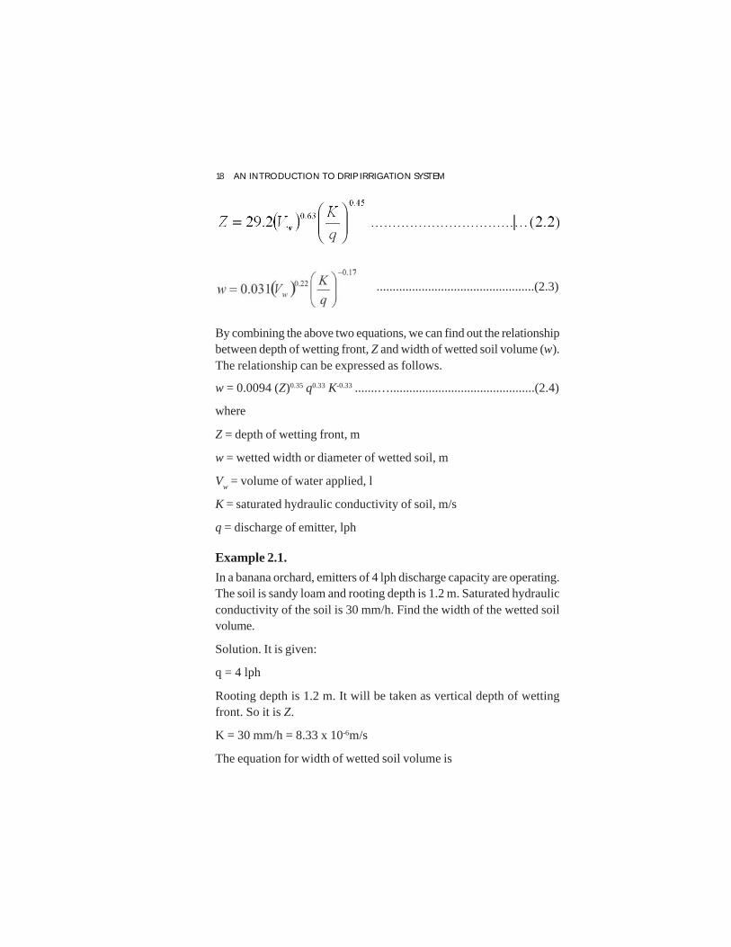
By combining the above two equations, we can find out the relationshipbetween depth of wetting front, Z and width of wetted soil volume (w).The relationship can be expressed as follows.
w = 0.0094 (Z)0.35 q0.33 K-0.33 .......….............................................(2.4)
where
Z = depth of wetting front, m
w = wetted width or diameter of wetted soil, m
Vw = volume of water applied, l
K = saturated hydraulic conductivity of soil, m/s
q = discharge of emitter, lph
Example 2.1.
In a banana orchard, emitters of 4 lph discharge capacity are operating.The soil is sandy loam and rooting depth is 1.2 m. Saturated hydraulicconductivity of the soil is 30 mm/h. Find the width of the wetted soilvolume.
Solution. It is given:
q = 4 lph
Rooting depth is 1.2 m. It will be taken as vertical depth of wettingfront. So it is Z.
K = 30 mm/h = 8.33 x 10⁻⁶m/s
The equation for width of wetted soil volume is


20 AN INTRODUCTION TO DRIP IRRIGATION SYSTEM
=1 0.60 0.754
0.60 0.60
× ×
× = 31.25% or 32%
Mohammed (2010) developed a simple empirical model to determinethe wetting pattern geometry from surface point source drip irrigationsystem. The wetted soil volume was assumed to depend on the saturatedhydraulic conductivity, volume of water applied, average change ofmoisture content and the emitter application rate. The followingassumptions were made.
• A single surface point source irrigated a bare soil with a constantdischarge rate.
• The soil is homogeneous and isotropic.
• No water table present in the vicinity of root zone.
• The evaporation losses are negligible.
• The effect of soil properties is represented by its porosity andsaturated hydraulic conductivity.
• The value of porosity equals the value of saturated moisturecontent. It could be obtained using an equation given by Hillel,(1982) which states:
−==
p
bSn
ρρθ 1 …..........................................................(2.6)
where,
n = porosity of the soil
θs = Moisture content at 0 bars
ρb = bulk density of the soil (measured)
ρp = particle density of the soil
It was considered that wetted radius and wetted depth of soil volumedepends upon certain variables. The functional relationship among allthe variables can be defined as follows:

DRIP IRRIGATION SYSTEMS 21
r ∝ f1 (K, n, qw, V
w).......…...........................................................(2.7)
z ∝ f2 (K, n, qw
, Vw).......…..........................................................(2.8)
where,
r = wetted radius
K = soil hydraulic conductivity
n = soil porosity
qw
= application rate
Vw
= volume of water applied
z = depth of wetted zone.
If we consider the equation given by Hillel (1982), the above twoequations can be written as
r ∝ f1 (K, θS , q
w , V
w)........…....................................................... (2.9)
z ∝ f2 (K, θ
S , q
w , V
w).......…..................................................... (2.10)
Ben-Asher et al. (1986) investigated the infiltration from a point dripsource in the presence of water extraction using an approximatehemispherical model. For infiltration from a point source without waterextraction, they established the following:
2Sθθ ≈∆ ….......................................................................... (2.11)
The new variable θ∆ is called the average change of soil moisturecontent. This leads to:
r ∝ f1 (K, ∆θ , qw
, Vw)......…..................................................... (2.12)
z ∝ f2 (K, ∆θ , q
w , V
w).......….................................................... (2.13)
According to the approaches introduced by Shwartzman and Zur (1986)and Ben Asher et al. (1986), the nonlinear expressions describingwetting pattern may take the general forms as:
r = ∆θα Vw
β qw
γ Kλ ...............…........................................................ (2.14)
z = ∆θρ Vw
σ qw
δ Kς…................................................................. (2.15)

22 AN INTRODUCTION TO DRIP IRRIGATION SYSTEM
Once they identified the model structure and order, the coefficientswere estimated in some manner. To determine the coefficients of Eq.2.14 and 2.15, four available published experimental data of Taghaviet al. (1984), Anglelakis et al. (1993), Hammami et al. (2002), and Liet al. (2003) were adopted. The choice of these experiments wasessentially based on availability of their convenient data. A nonlinearregression approach was used to find the best-fit parameters for theEq. 2.14 and 2.15. The following equations are obtained:
r = ∆θ -0.5626Vw
0.2686 qw
-0.0028 K-0.0344…............................................ (2.16)
z = ∆θ-0.383 Vw
0.365 qw
-0.101 K 0.1954 …............................................. (2.17)
where, r and z (cm) are consistent units used in this approximations,V
w (ml), q
w (ml/h), and K in (cm/h).
Cook et al. (2006) developed a model and implemented in the WetUpsoftware which uses data on the approximate radial and vertical wettingdistances for different soils and discharge rates estimated by usinganalytical methods. WetUp is an easy to use and freely availablesoftware tool (http://www.clw.csiro.au/products/wetup), which willdefinitely help to graduate students to fine tune their research work oncrop water management under drip irrigation systems. The program isa results of collaborative efforts among the Commonwealth Scientificand Industrial Research Organization (CSIRO), Cooperative ResearchCentre (CRC) for Sustainable Sugar Production and the NationalProgram for Irrigation Research and Development (NPIRD) inAustralia and the methods described by Thorburn et al. (2002). Youcan not provide the manual inputs but can always select all the requiredinputs from pre-defined selection boxes and drop down menus. Everysimulation window opens with predefined values and the user can easilyadjust or select the soil type, emitter flow rate, the maximum time andwhether a surface or buried emitter should be simulated starting underdry, moist or wet soil condition. Different soils can be chosen by doubleclicking on the ‘Select Soil Type’ section on the simulation windows,or by choosing an appropriate button in the button bar. There arecurrently 29 soils which are based on average soil properties publishedby Clapp and Hornberger (1978) and measured field soils from

DRIP IRRIGATION SYSTEMS 23
Queensland in Australia published by Verburg et al. (2001). Flow ratesmay be selected in the range of 0.5 to 2.7 l/hr for an irrigation time of1 to 24 hours. The depth of buried drip lines may be changed in therange of 0.1 to 1.5 m. In Indian conditions, we normally use 4 to 8 lphemitters. Since only 29 soils have been included, you may not findyour soils and hence this is a limitation. However, suppose you wantto simulate wetting patter of 4 lph emitter after 12 hrs, then you canthink of using emitter of 2 lph and simulate it for 24 hrs. This softwareis meant as an educational tool and you can at least see the effect ofchanging the variables on wetting patterns.


3Components of Drip Irrigation
Systems
A drip irrigation system consists of the components such as pump unit,fertigation equipment, filters, main, sub-main, laterals, and distributoryoutlets (emitters, micro-sprinklers, bubblers, etc.). Here we areconcerned about drip system so we will talk about emitters in thefollowing discussion. Besides, gate valves, check valves, pressuregauges and flow control valves are also used to regulate the flow ofwater and serve as additional components. Several major componentsof drip irrigation system are shown in Fig. 3.1. The components ofdrip irrigation system can be grouped into two major heads as
i) Control head and
ii) Distribution network
3.1. Control Head
The control head of drip irrigation system includes the pump or overheadtank, fertigation equipment, filters, and pressure regulator.
3.1.1. Pump/Overhead Tank
It is required to provide sufficient pressure in the drip irrigation system.Centrifugal pumps are generally used for low pressure drip irrigationsystems. Overhead tank is generally used for small areas of orchardcrops with a comparatively less water requirement.

26A
N IN
TR
OD
UC
TIO
N T
O D
RIP IR
RIG
AT
ION
SYST
EM
Fig. 3.1: Typical layout and the components of drip irrigation system(Source. Jain irrigation systems.)

COMPONENTS OF DRIP IRRIGATION SYSTEMS 27
The drip irrigation system requires energy to move water through thedistribution pipe network and discharge it through emitters. In mostirrigation systems, energy is imparted to water by a pump that in turnreceives its energy from either an electric motor or an internalcombustion engine. Therefore, it is important that both the pump andthe engine be well suited to satisfy the requirements of the irrigationsystem. Usually, centrifugal pumps are used for this purpose. Thecharacteristic curves of the pump are considered in selection of pumps.The characteristic curves show the relationship between capacity, head,power and efficiency of the pump. The head–capacity curve will givedischarge of a pump at a given head. As the discharge increases, thehead decreases. The pump efficiency increases with an increase indischarge but after a certain discharge, efficiency decreases. The BHPcurve for a centrifugal pump increases over most of the range as thedischarge increases. The pump horsepower at a maximum efficiencywould be determined from the characteristic curves based on theirrigation system design discharge and the total dynamic head againstwhich the pump is to operate. The total discharge and total dynamichead will be discussed later in this book. The following points shouldbe considered for installation of a centrifugal pump.
• The pump should be installed as close to the water source aspossible.
• Foundations should be rigid enough to absorb all vibrations.
• The pump and driver must be aligned carefully.
• On the belt drive units, the pump and driver shaft must beparallel.
• The site selected should permit the use of minimum possibleconnections on suction and delivery pipes.
• Suction and delivery pipes should be supported independentlyof the pump.
• The suction pipe should be direct and short.
• The size of the suction pipe should be such that the velocity ofwater does not exceed 3 m/s.

28 AN INTRODUCTION TO DRIP IRRIGATION SYSTEM
3.1.2. Fertigation
Fertigation means to apply fertilizers with the irrigation water.Chemical fertilizers are applied whenever needed by the crop in theappropriate form and quantity. The promotion of efficient, and effectivewater and fertilizer use is identified as an important contribution tothe strategy needed to address problems of water scarcity and practicingintensive agriculture. Improving the water and consequently fertilizeruse efficiency at farmers level, is the major contributor to increasefood production and reverse the degradation of the environment oravoid irreversible environmental damage and allow for sustainableirrigated agriculture. Fertigation was proposed as a means to increaseefficient use of water and fertilizers, increase yield, protect environmentand sustain irrigated agriculture. Achieving maximum fertigationefficiency requires knowledge of crop nutrient requirements, soilnutrient supply, fertilizer injection technology, irrigation scheduling,and crop and soil monitoring techniques.
Fertigation is directly related with improved irrigation systems andwater management. Drip and other micro-irrigation systems, highlyefficient for water application, are ideally suited for fertigation. Water-soluble fertilizers at concentrations required by crops are conveyedthrough the irrigation systems to the wetted volume of soil. Thus thedistribution of chemicals in the irrigation water will likely place thesechemicals in the root zone which helps the plants to uptake of N, P andK effectively. Many studies have been undertaken nationally andinternationally to determine the effect of fertigation method on growthand yield of several fruits and vegetable crops. Shedeed et al. (2009)evaluated the effect of method and rate of fertilizer application underdrip irrigation system on growth, yield and nutrient uptake by tomatogrown on sandy soil. The experiment was laid out in a randomizedcomplete block design having five treatments replicated three times in4.5m × 12m plot and included: control, normal fertilizers applied tosoil with furrow irrigation, normal fertilizers applied to soil with dripirrigation, ½ soil - ½ fertigation, ¼ soil - ¾ fertigation and 100%NPK fertigation as water soluble fertilizers applied through dripfertigation. They concluded that the fertigation at 100% NPK recorded

COMPONENTS OF DRIP IRRIGATION SYSTEMS 29
significantly higher total dry matter (4.85 t/ha) and leaf area index of3.65, respectively, over normal fertilizer applied to soil with dripirrigation. It was also observed that the drip fertigation had the potentialto minimize leaching loss and to improve the available K status in theroot zone for efficient use by the crop. Drip fertigation helped inalleviating the problem of K deficiency in the sandy soil. Frequentsupplementation of nutrients with irrigation water increased theavailability of N, P and K in the root zone and which in turn influencedthe yield and quality of tomato.
3.1.2.1. Advantages
The salient advantages of fertigation are given below:
• Uniform distribution of the nutrients in the soil by the irrigationwater.
• Deep penetration of the nutrients into the soil.
• Lower fertilizer losses from the soil surface.
• Better coordination of nutrient supply with the changing cropnutrient requirements during the growing cycle.
• Higher application efficiency.
• Full control and precise dosing of fertilizers in automatic andsemi-automatic irrigation systems avoids the leaching ofnutrients beneath the root zone.
• Avoiding of mechanized fertilizer broadcast eliminates soilcompaction and damage to the plants and the produce.
• Fertigation contributes to labor saving and convenience infertilizer application.
• Improves soil solution conditions
• Flexibility in timing of fertilizer application
3.1.2.2. Limitations and precautions
The limitations and precautions of using chemicals/fertilizers with dripirrigation are given below:

30 AN INTRODUCTION TO DRIP IRRIGATION SYSTEM
• Only completely soluble fertilizers are suitable to be appliedthrough the irrigation system.
• Acid fertilizers can corrode metallic components of the irrigationsystem.
• The immersed fertilizers can raise the water pH and trigger theprecipitation of insoluble salts that will clog the emitters andthe filtration system.
• Operation and maintenance requires skilled manpower.
• Health hazard exists if the irrigation water system is connectedto the drinking water supply network. Failure in the water supplymay cause the back flow of water containing fertilizers into thedrinking water system.
• The operator is exposed to burn injury by acid fertilizer solutions.
• To avoid the corrosion of metal parts, the pure water should beused in the last minutes of each irrigation cycle to wash theirrigation system from residual chemicals.
3.1.2.3. Fertigation Methods
The drip irrigation system employs injection devices for injecting thefertilizer into irrigation water. The injection device must ensure supplyof constant concentration of fertilizer solution during the entireirrigation period. The common methods of applying chemicals/fertilizers through the drip irrigation system are pressure differential,injection pump, and venturi appliance as shown in Fig. 3.2-3.4. Inpressure differential systems as shown in Fig. 3.2., a pressure drop iscreated by pressure reducing valves provided between the inlet andthe outlet of the supply tank. The pressure difference causes waterflow through the tank and then chemicals/fertilizers from the tank arecarried to the drip system. The tank contains solid soluble or liquidfertilizer that is dissolved gradually in the flowing water. Thedisadvantage of this type of injection system is that the concentrationof fertilizer is diluted as injection continues. There are no moving partsand hence prolong its working life. The system is simple in operationand involves no extra cost.
COMPONENTS OF DRIP IRRIGATION SYSTEMS 31
In injection pump method, the fertilizer solution is injected by means ofan injection pump (Fig. 3.3.). A pump can be driven by electric motor,diesel engine, or hydraulically operated by the water pressure of theirrigation system. The hydraulic pump is versatile, reliable and has lowoperation and maintenance expenses. A pump must develop a pressuregreater than that of in irrigation pipeline. Centrifugal pumps are usedwhen high capacity injection is needed. Fertigation pumps can becontrolled by the automatic irrigation system. The discharge of the pumpis monitored by means of a pulse transmitter that is mounted on thepump and converts its piston or diaphragm oscillation into electricalsignals. This system is flexible and can provide higher discharge rateand also does not create any further head loss in the irrigation system. Itmaintains a constant concentration of fertilizer solution throughout theapplication time. High cost of pump and its accessories, and operationand maintenance cost are its major disadvantages.
In venturi appliance, the fertilizer is injected through a constrictedwater flow path. A venturi injector is a tapered constriction whichoperates on the principle that a pressure drop results from the changein velocity of the water as it passes through the constriction. The velocityof water flow in the constricted section is increased. The pressure dropthrough a venturi must be sufficient to create a vacuum relative toatmospheric pressure in order to suck the solution from a tank into theinjector. A tube mounted in the constricted section sucks fertilizersolution from an open fertilizer tank. A venturi injector does not requireexternal power to operate. There are no moving parts, which increasesits life and decreases probability of failure. The injector is usuallyconstructed of plastic, which makes it resistant to most chemicals. Itrequires minimal operator attention and maintenance, and its cost islow as compared to other equipment of similar function and capability.It is easy to adapt to most irrigation systems, provided a sufficientpressure differential can be created to suck the fertilizers. It is possibleto inject nutrients in non-continuous (bulk) or continuous (concentration)fashion. For bulk injection, drip irrigation systems should be brought upto operating pressure before injecting any fertilizer or chemical. Fertilizershould be injected in a period such that enough time remains to permitcomplete flushing of the system without over-irrigation.

32 AN INTRODUCTION TO DRIP IRRIGATION SYSTEM
Fig. 3.2: Pressure differential system in closed fertilizer tank
Fig. 3.3: Fertilizer injection methods by pump injection (Lamm et al., 2001)

COMPONENTS OF DRIP IRRIGATION SYSTEMS 33
3.1.2.4. Fertigation Recommendations
For optimum plant growth and yield performance under fertigation,all fertilization-irrigation-input factors must be kept in mind so thatnone impose a significant limit. Implementing a fertigation program,the actual water and nutrient requirements of the crops, together witha uniform distribution of both water and nutrients, are very importantparameters. Crop water requirements are the most critical link betweenirrigation and a good fertigation. The amount of irrigation water forentire growing season must be precisely estimated under the prevailingclimatic conditions of the region under consideration. The mainelements for formulating and evaluating the fertigation program arecrop nutrient requirement, nutrients availability in the soil, the volumeof soil occupied by the crop rooting system and the irrigation method.Fertigation with drip irrigation, if properly managed, can reduce overallfertilizer and water application rates and minimize adverseenvironmental impact (Papadopoulos, 1993).
Fig. 3.4: Fertilizer injection methods by venturi (Metwally, 2001).

34 AN INTRODUCTION TO DRIP IRRIGATION SYSTEM
In general, empirical fertilization is based on farmer’s experience andon broad recommendations. The rate of nutrient application isdetermined by the nutrient requirement of the crop, the nutrientsupplying power of the soil, the efficiency of nutrient uptake and theexpected yield. These factors should be taken into consideration andfor the same crop, for each field, different fertigation programs arerecommended. The information on quantities of nutrients removed bycrop can be used to optimize soil fertility level. Part of the nutrientsremoved by crop is used for vegetative growth and the rest for fruitproduction. It is important to have enough nutrients in the rightproportions in the soil to supply crop needs during the entire growingseason. Vegetable crops differ widely in their macronutrientrequirements and in the pattern of uptake over the growing season. Ingeneral, N, P, and K uptake follow the same course as the rate of cropbiomass accumulation. Fruiting crops such as tomato, capsicum, andmelon etc. require relatively little nutrition until flowering and nutrientuptake accelerates and reaches to peak during fruit set and early fruitbulking. Fertilization recommendations, based on research conductedregionally, vary among areas of the country. It is important to recognizethese regional differences. Most of the Agricultural Universities inIndia have their own Regional Research Station or Krishi VigyanKendra. The relevant research findings of these research stations mustbe utilized while formulating fertigation programs
Further, using a standard drip fertigation program without soil testingwill often lead to wasteful fertilizer application or may results in anutrient deficiency. A soil test helps to estimate the nutrient supplyingpower of a soil and reduce guesswork in fertilizer practices. Soil testinglaboratories normally suggest ways to collect the soil samples. We areconcerned here with drip irrigation systems so the sampling must bedone accordingly. The place and depth of soil sampling relative to thedrippers is a sensitive issue of particular importance. Usually it isrecommended to get samples beneath the dripper, between the drippersand between the lateral pipes. In order to estimate the nutrient supplyingcapacity of a soil, apart from soil analysis, the parameters such asdepth of the crop rooting system, percentage of soil occupied by the

COMPONENTS OF DRIP IRRIGATION SYSTEMS 35
root system under different irrigation systems, and soil bulk densityare needed. These parameters are used to calculate the weight of soilof a certain area to a depth where the active rooting zone of the crop isdeveloped and estimate the reserves available nutrients for the crop.The appearance, growth and depth to which roots penetrate in soilsare in part species properties. For drip irrigated greenhouse vegetableslike tomato, cucumber, and capsicum, the wetted soil volume is usually30-50% of total soil volume. The fraction of soil occupied by rootsmust be taken into account whenever the amount of available nutrientsis calculated; otherwise the available amounts could be overestimated.In calculating the nutrient supplying capacity of a soil, the whole amountof the available nutrient to full depletion of soil can be taken intoconsideration. However, it is preferable that a certain amount of anutrient be reserved in soil. For intensive irrigated agriculture as safetyamounts of P and K in soil could be considered the 30 and 100 ppm,respectively. Moreover, in case that a nutrient is below the safety value,the fertilization program may include an amount of nutrient needed tobuild up soil fertility up to the safety margin. Theses margins are at thesame time the pool for increased demand in nutrients at eventual cropcritical nutrient stages. It should be emphasized that the amount offertilizer nutrients needed by the crop and the amount of nutrients,which should be applied, are not equivalent. The crop does not use allthe nutrients supplied by fertilizers, therefore, the actual amount appliedis higher than the amount required by the crop. In general, the higherthe water use efficiency of an irrigation system, the higher is the nutrientuptake efficiency. For a well designed drip irrigation system and withgood scheduling of irrigation, depending on soil type, the potential N,P and K uptake efficiency ranges between 0.75-0.85, 0.25-0.35 and0.80-0.90, respectively.
The capacity of the injection system depends upon the concentration,rate and frequency of application of fertilizer solution. The amount offertilizer to be applied per application (P) can be calculated by
................................................................. (3.1)


COMPONENTS OF DRIP IRRIGATION SYSTEMS 37
3.1.2.5. Plant Nutrients
The nutritional elements of plant are divided into two groups
i) Macro elements: This group includes elements that are consumedby plants in relatively high amounts. The common macroelements are nitrogen, phosphorous, potassium, calcium,magnesium and sulfur.
ii) Micro elements: This group includes elements that are alsoessential for good development of plants, but they are absorbedand used by plants relatively in small quantity. Common microelements are iron, manganese, zinc, copper, molybdenum andboron.
The functions of plant nutrients which support the plant system arebriefly discussed below:
Nitrogen (N): The nitrate form of nitrogen is not held in soils. Nitratesmove with other soluble salts to the wetted front. This is of particularinterest since NO
3-N should always be applied with irrigation and at
desired concentration needed by the crop to satisfy its nitrogenrequirement from one irrigation event to the other. Under irregularNO
3-N application, the fertigated crops might be under the over-
fertilization stage at the day of fertilizer application and under deficientstage due to leaching following the irrigation without fertilizer. Theammonium form of N derived from ammonium or urea fertilizers doesnot leach immediately because it is temporarily fixed on exchangesites in the soil. Ammonium and urea, however, may induceacidification, which may create higher solubility and movement ofPhosphrous in the soil. Urea is a highly soluble, chargeless molecule,which easily moves with the irrigation water and is distributed in thesoil similarly to NO
3. At 250C, it is hydrolyzed by soil microbial
enzymes into NH4 within a few days.
Phosphorous (P): Phosphorous is essential for cell division and plantroot development. It enhances flowering at the reproductive stage andis essential for development of seeds and fruits and necessary formeristematic division. Contrary to N and K, phosphorus is readily

38 AN INTRODUCTION TO DRIP IRRIGATION SYSTEM
fixed in most of the soils. Movement of P differs with the form offertilizer, soil texture, soil pH and the pH of the fertilizer. Phosphorusmobility in soil is very restricted due to its strong retention by soiloxides and clay minerals. Soil application of commonly available Pfertilizers generally results in poor utilization efficiency mainly becausephosphate ions rapidly undergo precipitation and adsorption reactionsin the soil, which remove them from the soil solution. Consequently,there is little or no movement of phosphate from point of contact withthe soil. Therefore, there is inefficient utilization of applied P fertilizers.Rauschkolb et al. (1976) found that P movement increases 5 to 10folds when applied through drip system, indicating that fertigation ofP is particularly important.
Potassium (K): The ionic form of this element is K+. Potassium takespart in activating enzymes involved in photosynthesis and in themetabolism for creating proteins and carbohydrates. The carbohydratesare transported from leaves to the roots and anions from roots to theleaves. It also assists in utilizing the water use by regulating the stomataand decreasing evaporation from the stomata. It improves the qualityof fruits and vegetables. It is less mobile than nitrate, and distributionin the wetted volume may be more uniform due to interaction with soilbinding sites. Drip irrigation systems apply K in both laterally anddownward direction, allowing more uniform spreading of the K in thewetted volume of soil. Application of K with the irrigation water isadvised since its effectiveness increases substantially and boost highercrop yield. Potassium can be applied as potassium sulphate, potassiumchloride and potassium nitrate. These potassium sources are solublewith little precipitation problems.
Calcium (Ca): The ionic form of calcium element is Ca++. This elementis involved in cell structure by creating calcium pectate and the celldivision. Calcium takes part in activating the reactions of some enzymessuch as phospholipase. It reacts as a detoxifying agent.
Magnesium (Mg): The ionic form of magnesium element absorbedby the plants is Mg++. Magnesium is the major element in chlorophyllstructure, which is responsible for photosynthesis process. It takes part

COMPONENTS OF DRIP IRRIGATION SYSTEMS 39
in activating some enzymes that are involved in carbohydratessynthesis. It enhances the uptake and translocation of phosphate.
Sulfur (S): The ionic form of this element absorbed by the plant isSO
4—. Sulfur is a components in the structure of some amino acids
such as cystine, cysteine and is active in protein structure. It is involvedin some enzyme oxidation and reduction reactions.
Iron (Fe): The ionic forms of this element absorbed by the plants areFe++ and Fe+++. This element is an important component in thechlorophyll synthesis in the plant. It is involved in enzymatic oxidationreduction reaction.
Manganese (Mn): It is activator in some enzymatic oxidation reductionreaction. It takes part in activating the enzymes that are responsiblefor reduction of nitrate-NO3
- to nitrite NO2-. It is involved in chlorophyll
synthesis and photosynthesis reactions.
Zinc (Zn): Zinc is involved in bio-synthesis of indole acetic acid (IAA).It is involved in enzymatic reactions.
Copper (Cu): Copper is involved in some enzymatic reductionreactions like ascorbic acid oxidase, phenolase, lactase etc.
Molybdenum (Mo): The ionic form of this nutritional element isMoO
4—. This activates enzymes that are responsible for the reduction
of nitrate NO3
- to nitrite NO2
-, therefore in molybdenum deficiencynitrate is accumulated in plant tissues. It is required by the rhizobiumbacteria for nitrogen fixation in legume.
Boron (B): The ionic form of this nutritional element is B4O
7—. Boron
activates certain enzymes and participates with sugars in producingcomplex compounds (lignine) that are responsible for the thickeningand hardening of cell walls. It participates in the process of producingthe rhizobium nodules that are responsible for the nitrogen fixation oflegume roots.
The fertilizer to be used for fertigation must be water-soluble (Table3.1). However, most of the common P and K fertilizers are notconvenient for fertigation due to their low solubility. This is particularlythe case with the P fertilizers.

40 AN INTRODUCTION TO DRIP IRRIGATION SYSTEM
Table 3.1: Solubility of fertilizers in water (kg/100 litters).
Type of fertilizer Solubility
Ammonium sulphate 71Ammonium nitrate 119Urea 110Monoammonium phosphate (MAP) 23Urea phosphate 96Potassium sulphate 7Potassium nitrate 32
Example 3.1. The nitrogen concentration of solid urea fertilizer is 46%. Prepare a solution of 80 ppm nitrogen.
Solution
The amount of urea to be dissolved in 1 m3 of water can be calculated by
fertilizerin element of
100elementofppm
%×
Example 3.2. The liquid ammonium nitrate has nitrogen concentrationof 18 % with specific weight of 1.23 g/cm3. Prepare a solution of 100ppm nitrogen.
Solution
The amount of liquid ammonium nitrate to be dissolved in 1 m3 ofwater can be calculated by
Example 3.3. A drip irrigation system is installed in 1 ha area undercitrus crop. The plants are spaced at 5 m ´ 5.5 m apart. Urea –ammonium nitrate, a liquid fertilizer with 32% nitrogen and weighing

COMPONENTS OF DRIP IRRIGATION SYSTEMS 41
1.32 kg/l is available for fertigation. Find the fertilizer injection rateto apply 40 kg/ha of elemental nitrogen. The irrigation and fertilizingtime are 8 hrs and 4 hrs respectively.
Solution
Irrigation application time (T) = 8 h,
Fertilizing time = 4 h,
The ratio of fertilizing time and irrigation application time (tr) = 4/8 =0.5
The concentration of elemental nitrogen, N, in the liquid fertilizer
C = 1.32 X 32/100 = 0.42 kg/l
Using Eq. 3.2, the injection rate
3.1.2.6. Sources of fertilizers
Commercial P-fertilizers may also precipitate in the irrigation pipenetworks and reacts with ions present in the irrigation water such asCa or Mg. Therefore, when choosing the P fertilizer for fertigation,besides solubility, we must take care to avoid P-Ca and P-Mgprecipitation in the irrigation lines and emitters. Keeping this in view,acid P fertilizers like phosphoric acid, urea phosphate ormonoammonium phosphate are recommended. Different sources offertilizers, including P fertilizers, have different effects on irrigationwater and soil pH. High pH values greater than 7.5 in the irrigationwater are undesirable. Calcium and Mg carbonate and orthophosphateprecipitations may occur in the lines and the drippers. In addition,high pH may reduce Zn, Fe and P availability to plants. The desiredpH is below 7 and most cultivated crops are grown in the range of 5.5-6.5. The pH of the irrigation water could be reduced or controlled byusing P acid or acid based fertilizers like urea phosphate andmonoammonium phosphate. The use of acid fertilizers in drip systemsmay be beneficial in many ways other than the direct benefit from theadded P, such as increased solubility of soil native P minerals, increased

42 AN INTRODUCTION TO DRIP IRRIGATION SYSTEM
availability of other nutrients and micronutrients and prevention ofclogging of the fertigation system.
The choice of fertilizer suitable for a specific application should be basedon several factors: nutrient form, purity, solubility, and cost. A variety offertilizers can be injected into drip irrigation systems. Soluble NPKfertilizers are available in the market which is appropriate for fertigationbut the price might be in certain cases the main constraint. Common Nsources include ammonium sulphate, urea, ammonium nitrate, urea-ammonium nitrate, calcium nitrate, magnesium nitrate and potassiumnitrate. Potassium can be supplied from potassium chloride, potassiumsulfate, potassium thiosulfate, or potassium nitrate. In case that salinityis a problem potassium chloride and potassium sulphate should beavoided. For phosphorus application, phosphoric acid, urea phosphateor ammonium phosphate solutions are used commonly. Monoammoniumor mono potassium phosphate is also available.
3.1.2.7. Nutrient Monitoring
It is essential to monitor the soil and plant nutrient status to ensuremaximum crop productivity. In conventional production, soil NO
3-N
testing is usually carried out before we plant. Since drip irrigationsystem provides the ability to add N as and when required, moreextensive NO
3-N monitoring is justified. Traditional soil laboratory
test offer the most complete and accurate information. There are severalalternative techniques to aid on-farm nitrogen measurement. Oneapproach is the use of soil solution access tubes, also called suctionlysimeters. The details are not being discussed here. The use of suctionlysimetry has serious limitations. There can be large spatial variability;one portion of a field may vary from another and, since NO
3-N moves
with the wetting front, there can be stratification of NO3-N within thebed. This problem can be minimized by using multiple lysimeters perfield, but that also increases the effort and the cost. Interpretation ofresults is also problematic.
In general, when NO3-N concentration in a root zone soil solution isfound greater than 75 mg/l, it indicates that sufficient N is available tomeet immediate plant needs. A lower NO
3-N concentration cannot be

COMPONENTS OF DRIP IRRIGATION SYSTEMS 43
interpreted directly as N deficiency, given the difficulty to obtain asample representative of the whole root zone. Reliance on soil NO3-Ntesting is appropriate early in the crop cycle, when crop N uptake rateis low and the detection of substantial residual NO
3-N can lead to
reduced additional N fertigation. By mid-season, crop uptake ratesincrease and soil NO3-N concentration correspondingly will changemore rapidly. Also, once an extensive root system is developed, manycrops can take up N in excess of crop needs. From mid-season untilharvest, plant tissue analysis should be the primary indicator of Nstatus, although soil testing still may be used to identify fields whereNO
3-N levels remain high enough to delay additional N application.
Conventional plant tissue analysis, in which tissue is dried, groundedand analyzed chemically in a laboratory, is the most accurate way todetermine crop nutrient status. Unfortunately, laboratory analysis ofdry tissue is relatively costly, and the time lag between sampling andobtaining results can be significant. In recent years there has beenincreasing interest in on-farm tissue testing, particularly for monitoringdrip-irrigated fields. On-farm monitoring usually involves the analysisof NO
3-N and K content of petiole sap; sap analysis for PO
4-P is
uncommon. Measurement techniques include colorimetric methods,NO
3-N or K test strips (Hochmuth, 1994), or ion-specific electrode
(Hartz et al., 1993; Vitosh and Silva, 1994). Although all methods canbe used successfully, the ion-specific electrode is the most commonlyused approach. The appropriate protocol for tissue collection, handling,and analysis is discussed by Hochmuth (1994).
3.1.3. Filtration System
The clogging of emitters is the main problem encountered in theoperation of drip irrigation systems. Filtering and keeping contaminantsout of the system are the main defense against the clogging caused bymineral and organic particles. Impurities in water can be classifiedinto three categories:
• Inorganic solid particles: sand, silt and clay and insolubleprecipitation.
• Living organisms such as algae, protozoa, bacteria, and fungi.

44 AN INTRODUCTION TO DRIP IRRIGATION SYSTEM
• Organic debris
Removal of above mentioned impurities is essential for efficient andtrouble-free operation of a drip irrigation system which necessitatesthe use of proper filters.
3.1.3.1. Selection of Filters
While selecting filters for the drip irrigation system, the followingfactors are considered.
• The physical quality of water such as the concentration andpattern of the impurities, suspended solids and organic matter.
• The chemical nature of water such as pH level, and presence ofsediments forming chemical elements and possible reaction withthe injected fertilizers when fertigation is applied.
• Discharge and allowable head losses in the system.
• Reliability and durability of the filters.
• Cost of the filter.
• The total surface area of the filtration element is very important.The filtration area needed for moderately dirt water is in therange of 60-150 cm2 for drip irrigation.
3.1.3.2. Types of filters
Settling Basins: Settling basins can remove suspended materialranging from sand (2000 mm) to silt (200 mm) in stream water beingused for irrigation. It removes large volumes of sand and silt. Basinsare constructed so that it could limit turbulence and permit a minimumof 15 minutes of retention time for water to travel from the basin inletto the pumping system intake. Longer retention time is required toallow the settling of smaller particles. A basin of 1.2 m deep, 3.3 mwide and 13.7 m long is required to provide a one quarter hour retentiontime for a 57 lps stream. Settling basin should be relatively long andnarrow to eliminate short circuit current that reduces effective retentiontime. If the source of water is ground water, settling basins should not

COMPONENTS OF DRIP IRRIGATION SYSTEMS 45
Fig. 3.5: Arrangements of gravels in media filter
be used but if canal water is being used for irrigation through dripirrigation systems, it may be of a great use.
Media Filter: Media filters are used when irrigating with watercontaining high organic load such as water pumped from open waterbodies or reclaimed water. It consists of fine gravel and sand of selectedsizes placed in a pressurized tank. Arrangement of laying gravels/sandis shown in Fig. 3.5. Media filters are not easily plugged by algae andcan remove relatively large amounts of suspended solids before cleaningis needed. It can retain particle sizes in the range of 25 to 200 mm. Ingeneral water flow rates through the filters should be in between 10 to18 lps per square meter of filtration surface area. Media filter shouldbe followed by a secondary screen filter to prevent carry over ofcontaminants following the backwashing process. Numbers designatethe sand media filter used in most drip irrigation filters: number 8 and11 are crushed granite, and numbers 16, 20, and 30 are silica sands.The mean granule size in microns for each media number is

46 AN INTRODUCTION TO DRIP IRRIGATION SYSTEM
approximately 1900, 1000, 825, 550 and 340 for number 8, 11, 16,20, and 30, respectively.
When the water flows from top of the filter, it goes down throughlayered bed and flows out at the bottom of the filter. The organicimpurities adhere to the surface of the media particles and accumulatein the filter tank. When too much dirt has been accumulated in thelayered bed, the pressure head loss across the filter is increased andthe accumulated dirt has to be backwashed in time in order to avoidthe excess head losses. Backwashing is a process of reversing thedirection of water flow through the filter and bypassing the effluentand its need can be detected by the pressure drop across the filter. TheAmerican Society of Agricultural Engineers recommends that thepressure drop in the media filter should not exceed 70 kPa. They donot remove very fine silt and clay particles as well as bacteria.
Centrifugal Filter: The best treatment of the water containing soilparticles is sedimentation of the particles by means of sand separators.Sand separators, hydrocyclones or centrifugal filters are synaminouswhich remove suspended particles that have specific gravity greaterthan 1.2. The centrifugal sand separator separates the sand and otherheavy particles from the water by means of centrifugal force of thetangentially entering water into a conic tank (Fig. 3.6). The sand isthrown by the centrifugal force against the conic wall, settled downand accumulated in a collector at the bottom. The collector is washedout manually when full. The clean water is emitted in a spiral motionthrough an outlet at the top of the separator. The diameters of the topand bottom of the conical shape in centrifugal filter are designed inaccordance with the flow of water. The centrifugal filters effectivelyremove large quantity of sand particles. They are placed often at theupstream of media or screen filters.
Screen Filter: Screen filters are fitted just after the pumping unit andno other filter is required if source of water is ground water. The casingis built of metal or plastic material. It has four apertures: water inlet,outlet, draining valve and cover. It consists of a screen made of metal,plastic, or synthetic cloth enclosed in a special house used to limit

COMPONENTS OF DRIP IRRIGATION SYSTEMS 47
Fig. 3.6: Centrifugal filter (Phocaides, 2000)

48 AN INTRODUCTION TO DRIP IRRIGATION SYSTEM
maximum particle size. Screens are classified according to the numberof openings per inch with standard wire size for each screen size (Table3.2). Most manufacturers recommend 100 to 200 mesh screens fordrip irrigation system. Normally, the discharge through the screens isless than 135 lps per square meter of screen openings. A standard 200mesh stainless steel screen has only 58% open area and equivalentnylon mesh with same size opening has only 24% open area. In screenfilter, the mesh size and the total open area determine the efficiencyand operational limits.
Table 3.2: Specifications of filter screens.
Mesh No. Hole size, micron Wire thickness, micron
40 420 25050 300 18880 177 119100 149 102120 125 86155 100 66
200 74 53
Therefore, it is important to consider the percentage of open area whensizing a filter for a given system discharge. It may be fitted in a serieswith the gravel filter in order to remove the solid impurities like finesand, dust, etc. from water. Screen filters are suitable to water withinorganic impurities. High load of organic and biological impuritiesmay clog the screen promptly. Like media filters, the screen filters canbe cleaned manually or automatically (Fig. 3.7).
Disk Filters: This is more suitable for water with mixed impurities ofinorganic solid particles and organic debris. The casing is made ofmetal or plastic material. The filtration element is made of stackedgrooved ring shaped disks, tightened together by a threaded cap. Wateris filtered as it flows through the grooves. Coarse particles are trappedon the external surface of the stack while finer particles and organicdebris adheres to the inner grooves. The discs are pressed togetherduring filtration and direction of flow is reversed during back flushingmode. The discs start a spinning motion and complete retained
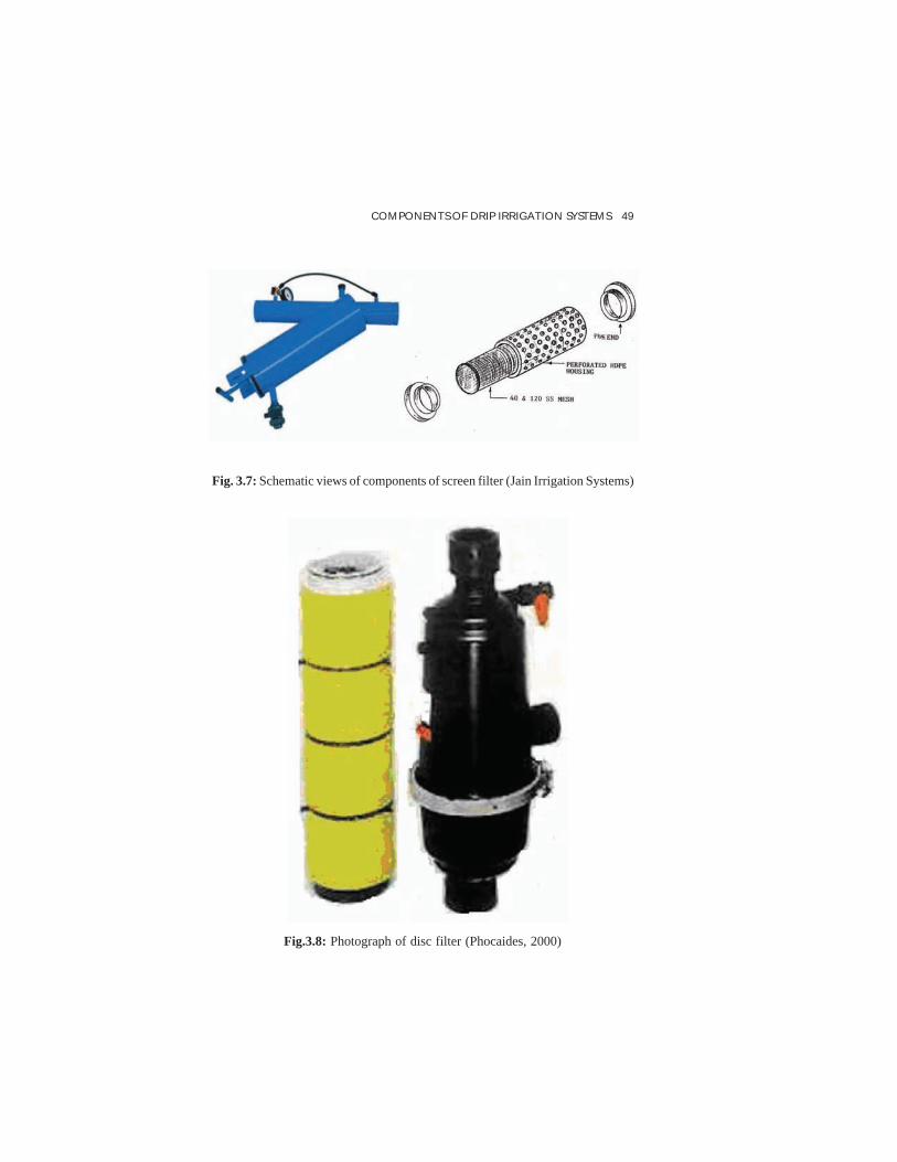
COMPONENTS OF DRIP IRRIGATION SYSTEMS 49
Fig. 3.7: Schematic views of components of screen filter (Jain Irrigation Systems)
Fig.3.8: Photograph of disc filter (Phocaides, 2000)

50 AN INTRODUCTION TO DRIP IRRIGATION SYSTEM
impurities are removed. The discs are assembled in a cylinder and arepressed together. To handle large flow rate, they can be installed inbatteries. The disk filters have much more higher dirt retention capacitythan screen filters with the same specifications. Such filters are oftenused as final filtering component before the water enters the system(Fig.3.8).
3.1.3.3. Filter characteristics and evaluation
The field evaluation of drip irrigation system includes a determinationof filtration efficiency and pressure differential across the filter. Theeffectiveness of the filtration system can also be indirectly assessedby evaluating the degree of emitter plugging. The filtration efficiency(F
r) of a filtration system is estimated by the following formula
where,
Sout
= the concentration of suspended solids (mg/l) in filter outlet, and
Sin = the concentration of suspended solids (mg/l) in filter inlet.
The water sample should be taken at least 30 minutes after the systemis turned on. The second aspect of field evaluation of filters in a dripsystem is differential pressure before and after filter backwashing takesplace. If the differential pressure is very high, a loss of flow can occurwhich affects the downstream pressure. Another approach fordetermining the effectiveness of the system is the extent of emitterplugging. A small percentage of emitter plugging can affect theuniformity of water application. Pressure regulators are generally usedto decrease the higher system pressure to the required system pressure.It controls the pressure in one way only i.e. high to low.
3.2. Distribution Network
The distribution network constitutes main line, sub-main line andlaterals with drippers and other accessories.

COMPONENTS OF DRIP IRRIGATION SYSTEMS 51
3.2.1. Main and Sub-main Line
A typical drip mainline is generally made of rigid Poly Vinyl Chloride(PVC) and High Density Polyethylene (HDPE). Pipes of 63 mm diameterand above with a pressure rating 4 to 6 kg/cm2 are generally used formainline pipes. The sub-main pipeline is made of rigid PVC, HDPE orLDPE (Low Density Polyethylene) of outside diameter ranging from 50to 75mm with a pressure rating of 2.5 kg/cm2. The diameters of mainand sub-main pipelines are chosen based on estimated water to be carriedout which ultimately needs the careful determination of peak crop waterrequirement. The sub-main line is connected to main line to deliver thewater to laterals. Gate valve is provided on the sub-main line to controlthe flow and practiced when irrigating large area divided in many sub-plots. Each sub-plot will be irrigated with one sub-main. Sub-main lineis fitted with a flushing valve to remove the contaminants. The main andsub-main lines are usually placed underground.
3.2.2. Laterals
Laterals are the pipes normally manufactured from LDPE or LinearLow Density Polyethylene (LLDPE). Generally, pipes having 12, 16and 20 mm internal diameter with a wall thickness varying from 1 to3mm are used as laterals. Nowadays even 32 mm lateral pipe is alsobeing used. Since laterals are always laid over the surface, it must beflexible and non-corrosive. Pressure variation within the laterals linesmust be within acceptable limits and therefore, selection of length anddiameter of lateral line is a matter of accurate design.
3.2.3. Drippers/Emitters
The emitters are connected to the laterals and control the flow of watercoming out of laterals. The design of single outlet emitter is based onthe principle of energy losses by sudden change in velocity of fluidflow in the emitter path. The successive change in velocity occurs dueto sudden enlargement and contraction in the designed flow path of thedisc element. The necessary arrangement for expansion of flow is doneby making larger cross sectional area in the shape of circle andcontraction of flow by smaller cross-sectional area in the shape of

52 AN INTRODUCTION TO DRIP IRRIGATION SYSTEM
rectangular channel. The bottom of the path is made flat to increasethe wetted perimeter of the flow passage, which leads to decrease thehydraulic radius and velocity of flow in the flow passage (Fig. 3.9).The energy losses occur when the flow channel suddenly expands to alarger diameter circular path. The energy loss is accomplished by twoways – first due to the impulse momentum which takes place as thewater flows from narrower rectangular passage to the wider circularpassage and secondly when the water flows from wider circular sectionto the narrower channel section. In this process, a lot of eddies areformed which causes a considerable dissipation of energy. The highpressure from the lateral line transmitted into the emitter is greatlyreduced and controlled flow of water emits in discrete drops almost atatmospheric pressure. Emitters are made from poly-propylene orpolyethylene and available in the market in different types and designs.
Fig. 3.9: Components of a point-source online pressure compensating dripper.

COMPONENTS OF DRIP IRRIGATION SYSTEMS 53
Point-source and line-source emitters operate either above or belowthe ground surface. Most of the point source emitters are either on-lineor in-line emitters. The primary difference between on-line and in-lineemitters is that the entire flow required downstream of the emitterpasses through an in line emitter. There is more head loss along alateral with on-line emitters than one with in-line emitters because ofobstruction created by the barbs of on-line emitters. The percentagearea wetted, and the reliability of the emitters against the clogging andmalfunctioning are two important aspects of quality and safety of dripirrigation systems. An ideal set of emitters should have the attributessuch as durability, low cost, reliable performance with a relativelylow rate of uniform discharge and relatively large and/or self-flushingpassageway to reduce or prevent clogging.
3.2.3.1. Types of Drippers/Emitters
(a) In-line Emitters: In-line emitters are fixed along with the lateralline. The pipe is cut and dripper is fixed in between the cutends, such that it makes a continuous row after fixing the dripper.They have generally a simple thread type or labyrinth type flowpath (Fig. 3.10).
(b) On-line Emitters: These are fixed on the lateral by punchingsuitable size holes in the pipe. These are of the following types:
i) Simple Type/Laminar Flow: In this type of dripper, thedischarge is directly proportional to the pressure. They havesimple thread type, labyrinth type, zig-zag path, vortex typeflow path or have float type arrangement to dissipate energy.
ii) Turbo Key Drippers: These are made of virgin and stabilizedpolymers and are available in 2, 4 and 8 lph discharge. Theyprovide resistance to blockage and are pressure compensating.
iii) Pressure Compensating Drippers: This type of dripper givesa fairly uniform discharge within the pressure range of 0.3atmospheres to 3.5 atmospheres. They are provided with a highquality rubber diaphragm to control pressure and are mostsuitable on slopes and difficult terrain.

54A
N IN
TR
OD
UC
TIO
N T
O D
RIP IR
RIG
AT
ION
SYST
EM
Fig. 3.10: In-line dripper

COMPONENTS OF DRIP IRRIGATION SYSTEMS 55
iv) Built-in Dripper Tube: In this system, polyethylene drippersare inseparably welded to the inside of the tube during extrusionof polyethylene pipes. They are provided with independentpressure compensating water discharge mechanism andextremely wide water passage to prevent clogging. Otheraccessories include take out/ starter, rubber grommet, end plug,joints, tees and manifolds.
3.2.3.2. Emitter discharge exponent
The flow from the emitter used in drip irrigation system is expressedby the following relationship:
q = Kd Hx .....….......................................................................... (3.5)
where, q is discharge rate of emitter in lph, Kd is discharge coefficient
which is a constant of proportionality, H is the pressure head at emitterin meter, and x is emitter discharge exponent. The value of x governsthe flow regime, and discharge and pressure relationship of an emitter.The pressure variation will less affect the discharge with lower valueof x. Normally x is taken as 0.5 for non compensating simple orificeand nozzle emitters. For fully compensating emitter, x = 0.0. Theexponent of long path emitter is normally varies from 0.7 to 0.8. Thevalues of x usually lie between 0.5 and 0.7 for tortuous path emitters.
3.2.3.3. Selection of an emission device
The selection of an emission device such as line-source and point-source emitters, micro- sprinklers and bubblers depends upon crop tobe irrigated, filtration requirement and soil type. The required emitterflow rate can be computed as follows:
where,
Qr = required emitter flow rate, l/h
di = water requirement of per plant, l/d
Ii = irrigation interval, day

56 AN INTRODUCTION TO DRIP IRRIGATION SYSTEM
It = irrigation time per set, h
Ea = application efficiency, fraction
N = number of emitters per plant
The crop water requirement under drip irrigation is different from thecrop water requirement under surface and sprinkler irrigation primarilybecause land area wetted is reduced resulting in less evaporation fromsoil surface. The capacity of emission device can be computed by usingequation
….................................................... (3.7)
where,
Q = capacity of emission device, l/h
A = area irrigated by the emission device, m2
d = depth of applied water, mm
H = hours of application of irrigation water
Tm = off time for maintenance, h
Ea = application efficiency, %
The area irrigated by an emission device is computed by the equation
…...... ..................................................... (3.8)
where,
A = area irrigated, m2,
L = spacing between adjacent plant rows, m
S = spacing between emission point, m
Wp = percent of cropped area being irrigated
Ne = number of emission devices at each emission point.
The value of Wpvaries from 30 to 100%, depending upon the type of

COMPONENTS OF DRIP IRRIGATION SYSTEMS 57
crop and its age. For widely spaced horticultural fruit tress (vine, bush,mango etc.), Wp varies between 30 to 60 % of area of each tree and forclose growing crops such as vegetables, the value of W
p is considered
as 100%. The number of emission devices per emission point,requiredfor desired wetting pattern is determined on the basis of horizontaland vertical movement of water through the soil. The soil moisturemovement studies are required to be conducted at several representativesites around the field to obtain horizontal and vertical spread data.
3.2.3.4. Emitter spacing
As we have discussed in Chapter-2 that wetting pattern of the emitterdetermines the spacing and number of emitter required per plant. Todetermine the wetted width and depth of water front, Mohammed(2010), Schwartzmass and Zurr (1985) and Wetup model can be used.United States Soil Conservation Services (1984) has provided anestimate of maximum horizontal wetted width from a single point sourceemitter and this can be used where field data are not available (Table3.3). For line-source emitter, this value must be multiplied by 0.8.
Table 3.3: Wetted width or diameter of wetted circle of a point source emitterof 4 lph capacity (United States Soil Conservation Services, 1984)
Depth of root zone and Homogeneous Soil profiles of varyingsoil texture soil layer, m textural group
Low density, m Moderatedensity, m
Root zone depth, 0.75 mCoarse soil 0.45 0.75 1.05Medium soil 0.90 1.20 1.50Fine soil 1.05 1.50 1.80Root zone depth, 1.5 mCoarse soil 0.75 1.40 1.80Medium soil 1.20 2.10 2.70Fine soil 1.50 2.00 2.40


4Estimation of Crop Water
Requirement
The quantity of water use by the crops is directly proportional to itsgrowth. Crops use water in transpiration. The root hairs extract waterfrom the soil and the water travels through the stem towards the leaves.The water transpires into the air through pores in the surface of theleaves. Water is also lost when it evaporates from the soil and othersurfaces. The combined loss of water through transpiration andevaporation is termed as evapotranspiration. Measurement of theevapotranspiration will tell you how much water you are required tosupply to the crop. The amount of water used by the crop will dependupon the type of crop and its stage of growth, soil types, andenvironmental factors such as sunlight, humidity, wind speed andtemperature. The crops grown in areas which are hot, dry, windy andsunny will require more water than crops grown in cool, humid andcloudy environment. The influence of the climate on crop waterrequirement is accommodated by the reference evapotranspiration(ETo
). It can be defined as the rate of evapotranspiration from a largearea, covered by green grass, 8 to 15 cm tall, which grows actively,completely shades the ground and which is not short of water. It isexpressed in mm per unit of time, e.g. mm/day or mm/month. Grasshas been taken as the reference crop.

60 AN INTRODUCTION TO DRIP IRRIGATION SYSTEM
4.1. Methods of Evapotranspiration Estimation
4.1.1. Direct Methods of Measurement of Evapotranspiration
4.1.1.1. Pan Evaporation Method
Evaporation pans provide a measurement of the combined effect oftemperature, humidity, wind speed and sunshine on the reference cropevapotranspiration. Many different types of evaporation pans are beingused. The best known pans are the Class A evaporation pan (circularpan) as shown in Fig. 4.1 and the Sunken Colorado pan (square pan).The evaporation pan is installed in the field or at the experimental siteand filled with a known quantity of water. The water depth in the panis to be recorded and the water is allowed to evaporate during 24 hours.After 24 hours, the remaining quantity of water or say water depthwill be measured. If the area receives any rainfall, that may be recorded.If the water depth in the pan drops too much, water is added and thewater depth is measured before and after the water is added. If thewater level rises too much water is taken out of the pan and the waterdepths before and after is measured. The amount of evaporation (E
PAN)
per time unit is calculated. This alone can not be considered as thewater requirement of the crops grown nearby areas. The E
PAN is
multiplied by a pan coefficient, KPAN
, to obtain the referenceevapotranspiration (ET
o).
ETo = K
PAN × E
PAN …............................................................... (4.1)
Fig 4.1: Class A evaporation pan

ESTIMATION OF CROP WATER REQUIREMENT 61
Determination of KPAN
It is obvious that the water in the evaporation pan and from the grassfield does not evaporate in a similar fashion under the same climate.Therefore a special coefficient is used (K
PAN) to relate one to the other.
The pan coefficient, KPAN
, depends on the type of pan used, the panenvironment, and the climate (humidity and wind speed). For a panplaced in a fallow area with high humidity and low wind speed, theK
PAN will be high. But if the pan is placed in a cropped area with low
humidity and higher wind speed, the KPAN
will be low. Normally forthe Class A evaporation pan, the K
PAN varies between 0.35 and 0.85.
Average KPAN
may be taken as 0.70. For the Sunken Colorado pan, theK
PAN ranges between 0.45 and 1.10, and average K
PAN is normally taken
as 0.80.
Example 4.1.
Class A evaporation pan is installed in a field and first day the waterdepth was recorded as 60mm and after 24 hours water depth becomes45mm. The day received no rainfall. If K
PAN is 0.70, find out the
reference evapotranspiration.
Solution. We know the formula to estimate reference evapotranspirationwhich is given hereunder.
ETo = K
PAN × E
PAN
Pan evaporation = 60-45 = 15mm
ETo = 0.70 × 15
=10.5 mm/day
Crop Coefficient
We are more interested in the estimation of crop water requirement sothat we can plan our irrigation scheduling and design of irrigation systems.Reference evapotranspiration gives the value for a short grass under agiven conditions. Here a coefficient is introduced which will considerthe specific crop and its different growth stages. This coefficient is calledcrop coefficient (K
c). If we know ET
o and K
c, then we can determine the
crop water requirement i.e. ETCROP
, as given below.

62 AN INTRODUCTION TO DRIP IRRIGATION SYSTEM
ETCROP
= Kc × ET
o …................................................................. (4.2)
The crop coefficient, Kc, depends on the type of crop, growing stages
and weather. A well developed tomato crop with full canopy coverwill transpire more water than the reference grass crop. The same cropduring initial stages may require less water than the reference grasscrop. I mean to say that the value of the crop coefficient ranges fromthe initial to final harvesting stages. Also in order to determine thevalue for any crop, knowledge about the length of the crop growingseason and the lengths of the various growth stages is essential. Foodand Agriculture Organization (FAO) has given all these informationbut it is better to collect the total length of growing season and theduration of the various growth stages of the crops from nearbyAgricultural University or Agricultural Research Station. The totalgrowing season has been divided into 4 growth stages: initial stage,crop development stage, mid-season stage, and the late season stage.Table 4.1 shows the total length of growing periods and duration ofthe various growth stages for some of the major field crops (FAO).Table 4.2 shows the average values for some crops according to itsfour different growth stages. Actually, the value also depends uponthe weather especially on the relative humidity and the wind speed.The values indicated in Table 4.2 should be reduced by 0.05 if therelative humidity is high (RH > 80%) and the wind speed is low (u <2 m/sec). The values may be increased by 0.05 for relative humiditylesser than 50% and the wind speed more than 5 m/sec.
Now, the values of crop coefficient can be taken from the table givenby FAO but growth stages are not confined on monthly basis. Forexample, crop development stage may range from January 15 toFebruary 20. How will you calculate the monthly crop coefficient?This we are going to explain with an example problem. Methods ofestimation of reference evapotranspiration will be discussed later inthis chapter.
Example 4.2.
Tomatoes are transplanted on 1st November and normally these areharvested up to March. The monthly evapotranspiration are given and

ESTIMATION OF CROP WATER REQUIREMENT 63
average relative humidity is around 80%. The prevalent wind speed is4m/s. Calculate the total crop water requirement of tomatoes.
Months November December January February MarchETo (mm/day) 5.0 4.5 4.0 6.0 6.5
Solution. Let us first determine the duration of various growth stages as follows.
Crops Total Initial Crop Mid-season Lategrowing growth development stage seasonseason stage stage stage
Tomatoes 145 30 40 50 25
We know that the total duration of crop is 145 days and date oftransplanting of tomatoes is 1st November, now total duration ofgrowing period can be written date wise in the following manner.
cK
values have been taken from Table 4.1 keeping in view that humidityand wind speed are normal.
Growth stages Date Kc values
Initial stage, 30 days 1 Nov – 30 Nov 0.45Crop development stage, 40 days 1 Dec – 9 Jan 0.75
Mid-season stage, 50 days 10 Jan – 29 Feb 1.15Late season stage, 25 days 1 Mar – 25 Mar 0.80
Last date of harvest 25 Mar —-
Table 4.1: Approximate duration of growth stages for various field crops.
Total Initial Crop Mid Latestage Development season season
stage stage stage
Barley/Oats/Wheat 120 15 25 50 30150 15 30 65 40
Bean/green 75 15 25 25 1090 20 30 30 10
Bean/dry 95 15 25 35 20
Contd.

64 AN INTRODUCTION TO DRIP IRRIGATION SYSTEM
110 20 30 40 20Cabbage 120 20 25 60 15
140 25 30 65 20Carrot 100 20 30 30 20
150 25 35 70 20Cotton/Flax 180 30 50 55 45
195 30 50 65 50Cucumber 105 20 30 40 15
130 25 35 50 20Eggplant 130 30 40 40 20
140 30 40 45 25Grain/small 150 20 30 60 40
165 25 35 65 40Lentil 150 20 30 60 40
170 25 35 70 40Lettuce 75 20 30 15 10
140 35 50 45 10Maize, sweet 80 20 25 25 10
110 20 30 50 10Maize, grain 125 20 35 40 30
180 30 50 60 40Melon 120 25 35 40 20
160 30 45 65 20Millet 105 15 25 40 25
140 20 30 55 35Onion/green 70 25 30 10 5
95 25 40 20 10Onion/dry 150 15 25 70 40
210 20 35 110 45Peanut/Groundnut 130 25 35 45 25
140 30 40 45 25Pea 90 15 25 35 15
100 20 30 35 15Pepper 120 25 35 40 20
210 30 40 110 30Potato 105 25 30 30 20
145 30 35 50 30Radish 35 5 10 15 5
Total Initial Crop Mid Latestage Development season season
stage stage stage
Contd.

ESTIMATION OF CROP WATER REQUIREMENT 65
40 10 10 15 5Sorghum 120 20 30 40 30
130 20 35 45 30Soybean 135 20 30 60 25
150 20 30 70 30Spinach 60 20 20 15 5
100 20 30 40 10Squash 95 20 30 30 15
120 25 35 35 25Sugarbeet 160 25 35 60 40
230 45 65 80 40Sunflower 125 20 35 45 25
130 25 35 45 25Tomato 135 30 40 40 25
180 35 45 70 30
Table 4.2: Values of the crop factor ( cK ) for various crops and growth stages.
Crop Initial stage Crop dev. Mid-season Late seasonstage stage stage
Barley/Oats/Wheat 0.35 0.75 1.15 0.45Bean, green 0.35 0.70 1.10 0.90
Bean, dry 0.35 0.70 1.10 0.30Cabbage/Carrot 0.45 0.75 1.05 0.90
Cotton/Flax 0.45 0.75 1.15 0.75Cucumber/Squash 0.45 0.70 0.90 0.75
Eggplant/Tomato 0.45 0.75 1.15 0.80Grain/small 0.35 0.75 1.10 0.65
Lentil/Pulses 0.45 0.75 1.10 0.50Lettuce/Spinach 0.45 0.60 1.00 0.90
Maize, sweet 0.40 0.80 1.15 1.00Maize, grain 0.40 0.80 1.15 0.70
Melon 0.45 0.75 1.00 0.75Millet 0.35 0.70 1.10 0.65
Total Initial Crop Mid Latestage Development season season
stage stage stage
Contd.

66 AN INTRODUCTION TO DRIP IRRIGATION SYSTEM
Onion, green 0.50 0.70 1.00 1.00
Onion, dry 0.50 0.75 1.05 0.85Peanut/Groundnut 0.45 0.75 1.05 0.70
Pea, fresh 0.45 0.80 1.15 1.05Pepper, fresh 0.35 0.70 1.05 0.90
Potato 0.45 0.75 1.15 0.85Radish 0.45 0.60 0.90 0.90
Sorghum 0.35 0.75 1.10 0.65Soybean 0.35 0.75 1.10 0.60
Sugarbeet 0.45 0.80 1.15 0.80Sunflower 0.35 0.75 1.15 0.55
Tobacco 0.35 0.75 1.10 0.90
Now you see that months and growing stages are not matching i.e.crop development stage is covering December and 9 days in Januaryand we have K
c values according to the crop development stages. This
has to be corrected in the following manner.
November: Kc = 0.45
December: Kc = 0.75
January: Kc = 15.1
30
2275.0
30
9 ×+×
= 1.07
February: Kc= 1.15
March: Kc= 0.80
Now we have monthly evapotranspiration and Kc values, we can
determine crop water requirement on monthly basis. All months areassumed to have 30 days as suggested by FAO.
ETCROP
= Kc × ET
o
November: ETCROP
= 5 x 0.45 x 30 = 67.5 mm/month
Crop Initial stage Crop dev. Mid-season Late seasonstage stage stage

ESTIMATION OF CROP WATER REQUIREMENT 67
December: ETCROP
= 4.5 x 0.75 x 30 = 101.1 mm/month
January: ETCROP
= 4 x 1.07 x 30 = 128.4 mm/month
February: ETCROP
= 6 x 1.15 x 30 = 207.0 mm/month
March: ETCROP
= 6.5 x 0.80 x 30 = 130.0 mm/month
After adding the monthly crop water requirement, total waterrequirement for tomato is obtained as 634 mm.
4.1.1.2. Soil Moisture Depletion Method
The soil moisture depletion technique is usually employed to determinethe consumptive use of irrigated field crops grown on fairly uniformsoil, where the depth of ground water is such that it will not influencethe soil moisture fluctuations within root zone. This technique involvesthe measurement of soil moisture of various depths in effective rootzone at a number of times throughout the crop growth period. Thegreater the number of measurements the more will be accuracy. Bysumming moisture depletion of each of the soil layer and for eachinterval for the growth period, ET can be determined as:
ERDBMM
U ii
n
i
+
−=∑
=
..1001
21 ….............................................. (4.3)
where,
U = moisture depleted from the soil profile at a certain interval, cm
M1 = moisture content (%) in ith layer at the time of first sampling
M2 = moisture content (%) in ith layer at the time of next sampling
Bi = bulk density of ith the layer, g/cm3
Dt = depth of the soil layer, cm
ER = effective rainfall, cm
For periods between irrigation day and sampling day, soil moisturedepletion is assumed to be equal to pan evaporation. Then water usedfor crop growth period is determined by adding moisture depleted ( iU )during all intervals:

68 AN INTRODUCTION TO DRIP IRRIGATION SYSTEM
PANC
n
iiCROP EUET +=∑
=1…........................................ (4.4)
here, EPANC
is cumulative pan evaporation between irrigation andsampling day.
Evaporation can be measured by using a lysimeter which givesadditional information on soil water balance. A lysimeter is a measuringdevice used to measure the amount of actual evapotranspiration. Byrecording the amount of precipitation and the amount lost through thesoil, the amount of water lost to evapotranspiration can be calculated.Lysimeters are of two types: Weighing and non-weighing. We havenot included the detail discussion on lysimeter.
4.1.2. Empirical Methods
4.1.2.1. Thornthwaite Method
This is a widely used method for estimating potential evapotranspiration,developed by Thornthwaite (1948) who correlated mean monthlytemperature with evapotranspiration as determined from water balancefor valleys where sufficient moisture water was available to maintainactive transpiration. This formula is based mainly on temperature andestimates of the unadjusted potential evapotranspiration (mm), calculatedon a monthly basis taking a standard month of 30 days and 12 hours ofsunlight/day and is given by
a
m
I
TET
=
_
0
1016 …................................................... (4.5)
where, m is the months 1, 2, 3…12, −
mT is the mean monthly air
temperature (0C), I is the heat index for the year, given by:
5.1_
5
∑=∑= m
m
TiI for m = 1, 2, 3….…12 …............... (4.6)
a is an empirical exponent which can be computed by the followingexpression

ESTIMATION OF CROP WATER REQUIREMENT 69
a = 6.7 × 10⁻⁷ × Ι3 − 7.7 × 10⁻⁵ × Ι2 + 1.8 × 10⁻² × Ι + 0.4 9 ........ (4.7)
Thornthwaite’s equation was widely criticized for its empirical naturebut also widely used. Because Thornthwaite’s method of estimatingET
O can be computed using only temperature, it has been one of the
most misused empirical equations in arid and semi-arid irrigated areaswhere the requirement has not been maintained (Thornthwaite andMather, 1955).The application of this method to computeevapotranspiration for short time periods usually leads to error becauseincoming radiations may not be reflected by short term temperatures.Compared to the Penman formula, Thornthwaite values tend toexaggerate the potential evaporation. This is particularly marked inthe summer months with the high temperatures having a dominant effectin the Thornthwaite computation, whereas the Penman estimate takesinto consideration other meteorological factors.
4.1.2.2. Blaney – Criddle Method
Blaney and Criddle (1950) proposed an empirical method, atemperature based approach for calculating potentialevapotranspiration. The method uses temperature as well as day lengthduration, minimum daily relative humidity, and daytime wind speed at2m height. The model is quite sensitive to the wind speed variable andsomewhat insensitive to the estimate of relative humidity. The preferredform of the equation reveals its strong empiricism and is given by:
ET0 = α + bf ….......................................................................... (4.8)
where,
f = p (0.46T + 8.13)….............................................................. (4.9)
α = 0.0043RHMIN - (n/N) - 1.41................................................. (4.10)
b = 0.82 - 0.0041RHMIN
+ 1.07 (n/N) + 0.066(Ud)- 0.006 (RH
MIN)
(n/N)- 0.0006 (RHMIN
) (Ud) …..................................................(4.11)
The variable p in Eq. 4.9 is the rario of actual daily daytime hours toannual mean daily daytime hours expresses as a percent, T is the meanair temperature in 0C, (n/N) is the ratio of actual to possible sunshinehours, RH
MIN is the minimum daily relative humidity in percent, and

70 AN INTRODUCTION TO DRIP IRRIGATION SYSTEM
Ud is the daytime wind at 2m in m/s.
4.1.2.3. HargreavesMethod
The Hargreaves equation is a temperature based method and gives anexpression for the reference crop evapotranspiration (Hargreaves andSamani, 1982,1985). It gives reasonable estimates of reference cropevapotranspiration because it takes into account the incoming solarradiation and the impact of radiation warming the surface. TheHargreaves equation takes the form;
ET0 = 0.0022 × R
A × δ
T0.5 × (Τ + 17.8) ….................................. (4.12)
where,
RA = mean extra-terrestrial radiation (mm/day)
δT = temperature difference of mean monthly maximum temperature
and minimum temperature for the month (0C).
T = mean air temperature (0C).
4.1.3. Micrometeorological Method
4.1.3.1. Mass Transport Approach
As we know that the evaporation depends on the incoming heat energyand vapor pressure gradient, which, in turn, depend on several weathervariables such as temperature, wind speed, atmospheric pressure, solarradiation, and quality of water. The whole process of evaporation iscomplicated. A complete physical model can not accommodate all thefactors which are not controllable and measurable. The mass-transferapproach is one of the oldest methods (Dalton, 1802; Meyer, 1915;Penman, 1948) and is still an attractive method for estimating freewater surface evaporation because of its simplicity and reasonableaccuracy. The mass-transfer methods are based on the Dalton equation,which, for free water surface, can be written as:
Eo = C (e
s - e
a)…...................................................................... (4.13)
where, Eo is free water surface evaporation, e
s is the saturation vapor
pressure at the temperature of the water surface, ea is the vapor pressure
ESTIMATION OF CROP WATER REQUIREMENT 71
in the air and C is aerodynamic conductance. The term ea is also equal
to the saturation vapor pressure at the dew point temperature. Theparameter C depends on the horizontal wind speed, surface roughnessand thermally induced turbulence. It is normally assumed to be largelydependent on wind speed, u . Therefore, Eq. 4.13 can be expressedas:
Eo = f(u) (e
s - e
a) …................................................................ (4.14)
where, f(u) is the wind function. This function depends on theobservational heights of the wind speed and vapor pressuremeasurements. Penman (1948) proposed the following variation ofthe Dalton equation.
Eo = 0.40 (e
s - e
a) (1+0.17 u
d) ….............................................. (4.15)
where,
Eo= potential evaporation, mm
es = saturation vapor pressure at the temperature of the water surface,
mm of Hg
ea = actual vapor pressure in the air, mm of Hg
ud = wind speed at 2m height, miles/day
Example 4.3.
Determine the potential evaporation with Penman equation. Thefollowing data set is given:
ea =11.50 mm of Hg
es =13.20 mm of Hg
ud= 45 miles/day
Solution. The potential evaporation can be calculated by the followingequation.
Eo = 0.40 (e
s - e
a) (1+0.17 u
d)
= 0.40 (13.20-11.50) (1+0.17×45)

72 AN INTRODUCTION TO DRIP IRRIGATION SYSTEM
= 0.68 ×8.65
= 5.88 mm/day
Example 4.4.
In a cropped field, five set of the micro-meteorological data wererecorded and given in the table. Compute the potential evaporation byusing the Penman Mass Transport Method.
Data Set Saturation vapor Actual vapor pressure, Wind speed at 2pressure, mm of Hg mm of Hg m height, miles/day
1. 12.0 10.8 40.52. 10.2 8.2 12.83. 8.6 7.6 30.84. 7.2 7.0 45.65. 10.4 9.2 42.0
Solution. Penman (1948) equation based on Mass Transport Approachis given hereunder. All the required inputs are given.
Eo = 0.40 (e
s - e
a) (1+ 0.17 u
d)
For data set 1.
Saturation vapor pressure at the temperature of the water surface,es= 12.0
mm of Hg
Actual vapor pressure in the air, ea = 10.8 mm of Hg
Wind speed at 2m height, ud = 40.5 miles/day
Now, applying the formula, we get
Eo = 0.40 (e
s - e
a) (1+0.17u
d)
= 0.40(12.0-10.8)(1+0.17*40.5)
= 3.78 mm/day

ESTIMATION OF CROP WATER REQUIREMENT 73
Similarly for other data set, the information is given in the table.
Data Set saturation Actual vapor Wind speed at Potentialvapor pressure, e
spressure, e
a2m height, u
devaporation, E
o
(mm of Hg) (mm of Hg) (miles/day) (mm/day)
1. 12.0 10.8 40.5 3.782. 10.2 8.2 12.8 2.543. 8.6 7.6 30.8 2.494. 7.2 6.5 45.6 2.45
5. 10.4 9.2 42.0 3.91
4.1.3.2. Aerodynamic approach
Evaporation from an open surface is a dynamic process, whose ratedepends on ability of wind and the humidity gradient in the air abovethe evaporating surface to remove water vapor away from theevaporating surface via aerodynamic processes. Thornthwaite andHolzman (1939) proposed the following equation which includedspecific humidity gradient and logarithmic wind profile.
where,
EO
= evaporation, mm/hr
Pa = density of air, kg/m3
κ = von Karman’s constant, 0.41
q2 and q1 = specific humidity in g/kg at heights z2 and z
2
u2 and u
1 = wind speed in m/s at heights z
2 and z
2
Example 4.5. Estimate the evaporation from field data collected inWest Bengal by using aerodynamic approach. The data are given below.
ρa = density of air = 1.3 kg/m3
κ = von Karman’s constant, 0.41
q2 and q1 = specific humidity in g/kg at heights z2 and z1
=6.90 and 8.75g/kg


ESTIMATION OF CROP WATER REQUIREMENT 77
and outgoing energy fluxes can be expressed as follows.
Rn = H + λE + G…................................................................. (4.20)
where,
Rn = energy flux density of net incoming radiation (W/m2)
H = flux density of sensible heat into the air (W/m2)
λE = flux density of latent heat into the air (W/m2)
G = heat flux density into the water body (W/m2)
To convert the above lE in W/m2 into an equivalent evapotranspirationin units of mm/d, λE should be multiplied by a factor 0.0353. Thisfactor equals the number of seconds in a day (86 400), divided by thevalue of l (2.45 x 10⁶ J/kg at 20°C). Density of water is assumed as1000 kg/m3. Penman (1948) combined energy balance approaches andturbulent transport of water vapor away from an evaporating surfacecan be given as
.
( )1
0+
+−
=γ
γs
EGRs
Ean
…..................................................... (4.21)
where,
Eo = evaporation from open water surface, mm/day
Rn = net radiation in water equivalent, mm/day
G = soil heat flux in water equivalent, mm/day
( )( ) ( )( )NnedTN
nRR aAn 90.010.092.055.046.032.01 4 +−−×+−= σα ..(4.22)
where,
α =Albedo
RA = mean monthly radiation outside the atmosphere in water equivalent,
mm/day

78 AN INTRODUCTION TO DRIP IRRIGATION SYSTEM
Ta = mean air temperature, 0K
s = slope of the saturation vapor pressure vs. temperature curve, mmof Hg/0C.
γ = psychometric constant (0.49 mm of Hg/0C)
n/N
= ratio of actual to maximum possible sunshine hours
σ = Stefan-Boltzman constant = 5.56 x 10⁻⁸ w/m2/K4 = 2.06 x 10⁻⁹
mm/day
ed= saturation vapor pressure of the atmosphere in mm of Hg at dewpoint temperature or actual vapor pressure.
Again
( )wd TTesweaMeanRH
ed −−=×= 49.0100
….............................. (4.23)
where,
ea= saturation vapor pressure at mean air temperature, mm of Hg
esw= saturation vapor pressure at wet bulb temperature (Tw) and dry
bulb temperature(Td), mm of Hg.
An aerodynamic component is explained by the following expression.
Ea = 0.35 (ea - ed) × (1+ 0.0098u2) ….................................... (4.24)
Here u2 is wind speed in miles/day at 2m height and u2 can be determinedas given below.
u2 = log 6.6 × u
h /log h ….......................................................... (4.25)
where,
uh = wind speed at miles/day at height ‘h’ in feet
Example 4.7. Estimate the net radiation in water equivalent with thehelp of following given collected data in the field by using Penmancombination method. This example is taken from Ram Nivaset al. (2002).
Mean air temperature, Ta = 16.10C
Mean relative humidity = 68.5%


80 AN INTRODUCTION TO DRIP IRRIGATION SYSTEM
Finally, determine Ea with the given equation.
( ) ( )20098.0135.0 uedeaEa +×−= ( ) ( )47.2190098.0164.67.935.0 ×+×−= = 1.07 x 3.15
= 3.37 mm/day
By using Eq. 4.21, evaporation from open water surface in mm/daycan be determined.
( )[ ]1769.1
37.30.062.1769.10 +
+−=E
= (1.769×1.62+3.37) /2.769
= 3.85 mm/day
4.1.5.2. Modified Penman Approach
Monteith (1963, 1964) introduced resistance terms into the Penman methodand proposed the following equation to estimate latent heat of evaporation.
( ){ } ( ){ }
++
−+−
=
a
c
apan
rrs
reaesCGRs
LE1
./
γ
γργ …........................................... (4.26)
where,
aρ = density of air, 1.3 kg/m3
Cp = specific heat of air at constant pressure, 1008 J/kg/0C
ra = aerodynamic resistance, s/m
rc = canopy resistance, s/m
= rs + 15
rs = stomatal resistance, s/m
( ) ( )[ ]LAI
rrrrr abadabad
s
+×= ................................................. (4.27)
where,

ESTIMATION OF CROP WATER REQUIREMENT 81
adr = adaxial resistance
rab
= abaxial resistance
LAI = leaf area index
ea = actual vapor pressure, mm of Hg
es = saturation vapor pressure, mm of Hg
Aerodynamics resistance (ra) is determined as follows.
( ){ }[ ]2
2ln
uk
zodzra
−= ......................................................... (4.28)
where,
z = height
d = zero plane displacement = 0.63z
zo = roughness parameter = 0.13z
u = wind speed at height, z
κ = von Karman’s constant (0.41)
Example 4.8. Determine the latent heat of evaporation by usingModified Penman Approach with the following data collected in thefield.
Net radiation, Rn = 282.0 W/m2
Soil heat flux, G = 10.1 W/m2
S/γ = 1.860 at 17.50C
Density of air, ρa= 1.3 kg/m3
Specific heat of air at constant pressure, Cp = 1008 J/kg/0C
Psychometric constant, γ = 0.49 mm of Hg/0C
Dry bulb temperature = 17.00C
Wet bulb temperature = 9.80C
Saturation vapor pressure, es = 5.0mm of Hg


ESTIMATION OF CROP WATER REQUIREMENT 83
= 505.734 + 567.013) / (2.86+2.95)= 186.06 W/m2
= 0.27 mm/hr
4.1.5.3. Van Bavel method
Van Bavel (1966) modified the Penman method and introduced a newterm ‘ VB ’, and proposed the following formula.
( )[ ]γ
γ+
×××+−=
s
daBLGRsLE Vn
….............................. (4.29)
( )
−
×
=2
0
2
ln zdz
u
P
kB a
V
ερ…........................................ (4.30)
where,
da = vapor pressure deficit, mm of Hg and is equal to difference of esand ea
P = air pressure, 0.75 mm of Hg
u = wind velocity, m/s
z = crop height, m
d = zero plane displacement
L = latent heat, J/kg, 2.346
zo = roughness parameter
ε = 0.622 (it is a ratio of molecular weight of water to molecular weightof dry air
4.1.5.4. Slatyer and Mcllroy Method
The Slatyer-McIlroy equations are based on evapotranspiration froma wet surface with minimum advection. This happens when the airabove a surface is saturated due to vapor exchange with the wet surface.They used wet bulb depression instead of vapor pressure deficit and

84 AN INTRODUCTION TO DRIP IRRIGATION SYSTEM
proposed the following modified equation.
( )0
a p zn
a
C DR GET s
s r
ργ
− = + +
….................................. (4.31)
where,
Dz= wet bulb depression at height ‘z’. It is a difference of dry and wet
bulb temperature.
Example 4.9. Determine the potential evapotranspiration by using theSlatyer and Mcllroy method with the flowing data.
Net radiation (Rn) = 310.0 W/m2
Soil heat flux (G) = 12.6 W/m2
Slope of the saturation vapor pressure vs. temperature curve, s = 0.91mmof Hg/0C
Psychometric constant, γ = 0.49 mm of Hg/0C
Density of air, aρ = 1.3 kg/m3
Specific heat of air at constant pressure, Cp= 1008 J/kg/0C
Aerodynamic resistance, ra = 14.30 s/m
Wet bulb depression (Dz) = 1.40C
Solution. Putting all the given values in Eq. 4.31
( )0
a p zn
a
C DR GET s
s r
ργ
− = + +
( )310 12.6 1.3 1008 1.4
0.910.91 0.49 14.30
− × × = × + +
= 0.91 (212.42) + 128.29
= 193.30 + 128.29
= 321.59 W/m2 = 0.48 mm/hr

ESTIMATION OF CROP WATER REQUIREMENT 85
4.1.5.5. Priestley and Taylor Method
The Priestley-Taylor model (Priestley and Taylor, 1972) is amodification of Penman’s theoretical equation. An empiricalapproximation of the Penman combination equation is made by thePriestley-Taylor to eliminate the need for input data other than radiation.The adequacy of the assumptions made in the Priestley-Taylor equationhas been validated by a review of 30 water balance studies in which itwas commonly found that, in vegetated areas with no water deficit orvery small deficits, approximately 95% of the annual evaporativedemand was supplied by radiation (Stagnitti et al., 1989). Priestleyand Taylor (1972) found that the actual evapotranspiration from wellwatered vegetation was generally higher than the equilibrium potentialrate and could be estimated by multiplying the ET
o by a factor (α)
equal to 1.26. They demonstrated that potential evapotranspiration isdirectly related to the equilibrium evaporation in the absence ofadvection and proposed the following equation.
( )γ
α+
−××=
s
GRsET n
0 ….................................................. (4.32)
where,α is the empirical constant and is taken as 1.26 for temperatureranging between 15-300C. Although the value vary throughout the day,there is general agreement that a daily average value of 1.26 isapplicable in humid climates (Shuttleworth and Calder, 1979). Morton(1983) observed that the value of 1.26, estimated by Priestley andTaylor, was developed using data from both moist vegetated and watersurfaces. Morton recommended as 1.32 for estimation from vegetatedareas as a result of the increase in surface roughness. Generally, thecoefficient for an expansive saturated surface is usually greater than1.0. This means that true equilibrium potential evapotranspiration rarelyoccurs; there is always some component of advection energy thatincreases the actual evapotranspiration. Higher values of ranging upto 1.74, have been recommended for estimating potentialevapotranspiration in more arid regions (ASCE, 1990).
Example 4.10. Estimate the potential evapotranspiration by using the

86 AN INTRODUCTION TO DRIP IRRIGATION SYSTEM
Priestley and Taylor method. The following data were collected andgiven below.
Net radiation (Rn) = 310.0 W/m2
Soil heat flux (G) = 12.6 W/m2
Slope of the saturation vapor pressure vs. temperature curve, = 0.91mmof Hg/0C
Psychometric constant, γ = 0.49 mm of Hg/oC
An empirical constant, α = 1.26
Solution. All the data required by the Priestley and Taylor method ofcomputing potential evapotranspiration are given, so it easier to putall the values in Eq.4.32
=
1.26×0.91×(310-12.6) 0.91+0.49
= 243.57 W/m2
= 0.36 mm/hr
4.1.6. Methods in Remote Sensing Technology
Canopy temperature can be determined with remote sensing and thisis used in energy balance models which provide reliable estimates ofevapotranspiration estimation. Thermal infrared radiation data recordedfrom radiometers or scanners provide an input to methods of estimationof ET
o. There are several methods such as Bartholic, Namken and
Wiegand model, Brown and Rosenberg Resistance model, Stabilitycorrected aerodynamic resistance model, Energy balance–Regressionmodel, and Soer model, which are being used to estimate ETo. We arenot discussing these models in details but all the methods usuallyemployed in remote sensing technology are basically based on energybalance equation which is expressed below.

ESTIMATION OF CROP WATER REQUIREMENT 87
Rn = H + LE + G
where,
Rn = net radiation, W/m2
H = sensible heat flux, W/m2
LE =latent heat flux, W/m2
G = soil heat flux, W/m2
4.2. Crop Water Requirement in Greenhouse Environments
Inadequate irrigation tends to waste water, nutrients and energy, andmay cause soil degradation by water-logging and salinisation. Underclosed spaces such as greenhouses, the predominant role of croptranspiration in decreasing the heat load during warmer periods is animportant reason to develop irrigation scheduling that allow themaximization of the transpirational fluxes. The main process involvingthe fate of water in the greenhouse is evapotranspiration, a processthat is driven by a constant inflow of energy. As the ultra violetstabilized plastic films, used in greenhouse construction, changeslocally the radiation balance inside the greenhouse by entrapping thelong wave radiation and creates a barrier to moisture losses, the cropwater requirement is reduced due to less evapotranspiration. Cropcultivation under greenhouse reduces evapotranspiration to about 70%of open field. It, thus, improves the water use efficiency relative tounprotected cropping (Stanghellini, 1993). It has also been reportedthat farming under greenhouse can save about 20-25% of watercompared to the open drip irrigated farming systems.
For representing the conditions inside the greenhouse, Stanghellini(1987) revised the Penman-Monteith model. Normally wind speedsare typically less than 1.0m/s. The Stanghellini model includes thecrop canopy and aerodynamic resistance terms as well as more complexcalculations of the solar radiation heat flux derived from the empiricalcharacteristics of short wave and long wave radiation absorption in amulti-layer canopy. A leaf area index is used to account for energyexchange from multiple layers of leaves on crops grown inside the

88 AN INTRODUCTION TO DRIP IRRIGATION SYSTEM
greenhouse. The equation to estimate potential evapotranspiration(ET0) takes the forms as given hereunder.
( )
++∆
+−∆×=
a
c
a
ptn
r
r
r
CVPDKGR
LAIET
1
..
1.20
γ
ρ
λ ….............................. (4.33)
( )R
pnsn r
TTCRR 0..252
07.0−
−=ρ
…................................ (4.34)
where,
….......................................................... (4.36)
LAI = leaf area index in m2/m2
Kt = time unit conversion (86400s/day for ET
o in mm/day)
rc = canopy resistance, s/m
Rns
= net short wave radiation (MJ/m2/day)
To = leaf temperature (0C)
ra = aerodynamic resistance, s/m
Cp = specific heat of air which equals to 0.001013 (MJ/kg/0C)
ρ = mean air density (kg/m3)
ε = water to dry molecular weight ration
γ = latent heat of vaporization (MJ/kg)
σ = Stefan-Boltzmann constant (MJ/m2/K-4/day)
rR = radiative resistance (s/m)

ESTIMATION OF CROP WATER REQUIREMENT 89
P = atmospheric pressure (kPa)
VPD = vapor pressure deficit (kPa)
4.3. Computer Models to Estimate Evapotranspiration
4.3.1. ETo Calculator
Reference evapotranspiration (ETo) is a climatic parameter and canbe estimated from available weather data. It explains the evaporatingpower of the atmosphere at a specific site and does not consider thecrop characteristics and soil factors. The ETo calculator softwareestimates reference evapotranspiration by using the FAO Penman-Monteith equation. This method closely approximates grass ETo andis a physically based model which incorporates both physiological andaerodynamic parameters. The input data is classified in 4 groups suchas air temperature, humidity, wind speed, and sunshine and radiation.You will need to create a file wherein you will be required to fill upthe temperature and humidity data. If you do not have the wind speeddata, you need to choose the options available such as light wind tostrong wind. The output data can be plotted and imported to someother crop growth simulation model such as AquaCrop model, alsodeveloped by FAO, directly as the input file. The ET
o calculator was
developed by Dr. Dirk Raes of Katholieke Universiteit Leuven, Belgiumin cooperation with Land and Water Division of FAO. Students mustdownload it from FAO website and practice it to observed how humiditytemperatures and wind speed are changing the plot of ET
o.
4.3.2. Cropwat
CROPWAT 8.0 has been developed by Joss Swennenhuis for the WaterResources Development and Management Service of FAO. CROPWAT8.0 is based on the DOS versions CROPWAT 5.7 of 1992 andCROPWAT 7.0 of 1999. CROPWAT 8.0 is a computer program forthe estimation of crop water requirements from climatic and crop data.The program also allows the development of irrigation schedules fordifferent management conditions and the calculation of water supplyscheme for varying crop patterns. All calculation procedures as usedin CROPWAT 8.0 are based on the FAO guidelines as laid down in the

90 AN INTRODUCTION TO DRIP IRRIGATION SYSTEM
publication No. 56 of the Irrigation and Drainage Series of FAO “CropEvapotranspiration - Guidelines for computing crop waterrequirements”. It can be easily downloaded from FAO website andtakes directly the input of reference evapotranspiration calculated fromETo calculator.
4.4. Computation of Crop water Requirement with Limited Wetting
In drip irrigation systems, only part of the soil surface is wetted andfor widely spaced crops, crop canopy coverage is also limited. It is notappropriate to consider the soil evaporation from the entire soil surfaceunder drip irrigation systems. Vermeiren and Jobling (1984) suggestedusing a correction factor (K
r) to take into the account of percentage of
crop canopy coverage of cultivated land. The relationship can beexpressed hereunder:
ETCROPCor
= Kr × ETCROP
.........….............................................. (4.37)
where, ETCROP
is corrected crop water requirement, Kr is correction
factor and ETCROP
is crop water requirement without considering limitedarea wetting. Keller and Bliesner (1990) developed the followingformula to estimate crop evapotranspiration or crop water requirementfor limited wetted areas.
where, Pd is percentage of crop canopy coverage.
Example 4.11. A drip irrigated tomato crop is at development stage andthe relative humidity is 70% with wind velocity of 2m/c. Crop canopycoverage is 60% and K
c value for development stage is 0.75. Take ET
o
as 5.2 mm/day and correction factor as 0.92. Compare theevapotranspiration estimation without area wetting, Vermeirn and Jobling(1984), and Keller and Bliesner (1990) method for limited area wetting.
Solution. Let us estimate the crop evapotranspiration when limitedarea concept is not being applied.

ESTIMATION OF CROP WATER REQUIREMENT 91
ETCROP
= Kc × ΕΤο
= 0.75 x 5.2
= 3.9 mm/day
When limited area concept is being applied, according to Vermeirnand Jobling (1984)
ETCROPCOr
= Kr × ET
CROP
= 0.92 x 3.9
= 3.59 mm/day
Finally, according to Keller and Bliesner (1990),
[ ]dCROPCROPCr PETET ×= 1.0
= 3.9 (0.1 x 60 )
= 3.02 mm/day


5Irrigation Scheduling
The increasing shortages of water and cost of irrigation are leading todevelop methods of irrigation that maximize the water use efficiency.The advent of precision irrigation methods such as drip irrigation hasplayed a major role in reducing the water required in agricultural andhorticultural crops, but also has highlighted the need to develop newmethods of irrigation scheduling. Irrigation scheduling aims to achievean optimum supply of water to the crops for productivity with soilwater content maintained at field capacity. Irrigation scheduling is thedecision of when and how much water should be applied to the cropsin a field. The purpose is to find out the exact amount of water to beapplied to the field and the irrigation interval. It saves water and energyand thereby increases irrigation efficiency. There are certain irrigationcriteria which are used to determine when and how much water to besupplied. The most common criteria are soil moisture content and soilmoisture tension. For example, suppose a farmer whose main objectiveis to maximize crop yield consider soil moisture content as the irrigationcriterion. He decides that when soil water content drops below 80percent of the total available soil moisture, irrigation should start. Soilmoisture content to trigger irrigation depends on the farmer’s goal,strategy, and water availability. The farmer will try to keep the soilmoisture content above the critical level. Thus, irrigation is appliedwhenever the soil water content level reaches the critical level. Thischapter deals with the question that when to irrigate the crop, howmuch of water will be needed that has been explained in the chapter onwater requirement of crops.

94 AN INTRODUCTION TO DRIP IRRIGATION SYSTEM
5.1. Advantages of Irrigation Scheduling
• Can supply water to the various fields to minimize crop waterstress and maximize yields.
• It can make maximum use of soil moisture storage.
• Increasing water use efficiency means reducing fertilizer cost.
• Increases net returns by increasing crop yield and quality.
• Minimizes waterlogging and reduces drainage requirements.
• Controls root zone salinity problems.
5.2. Methods of Irrigation Scheduling
5.2.1. Water Balance Approach
The water balance approach to irrigation scheduling keeps the accountof all water additions and subtractions from the soil root zone. As thecrop grows and extracts water from the soil to satisfy itsevapotranspiration requirement, the soil water storage is graduallydepleted. The water requirement of the crop can be met by stored soilwater, rainfall, and irrigation. Irrigation is required when crop waterrequirement exceeds the supply of water from soil water and rainfall.The water balance method of irrigation scheduling is a method whichestimates the required amount and timing of irrigation for crops. Thismethod needs the prior information on initial soil water content in theroot zone, crop evapotranspiration, rainfall, and the available watercapacity of the soil. The available water capacity or total availablewater of the soil is the amount of water available for plants to use inbetween the field capacity and permanent wilting point. The netirrigation requirement is the amount of water required to refill the soilwater content of root zone to field capacity. This amount is the differencebetween field capacity and present soil water content and called thesoil water deficit (D
C). On a daily basis, D
C can be determined by
using the following equation:

IRRIGATION SCHEDULING 95
DC = D
P + ET
CROP - R - I
RR _ U + S
RUNOFF + DP ….................... (5.1)
where,
DP= soil water deficit on the previous day,
ETCROP
= crop evapotranspiration rate for the current day,
R = total rainfall for the current day,
IRR
= net irrigation amount infiltrated into the soil for the current day,
U = upflux of shallow ground water into the root zone,
SRUNOFF
= surface runoff,
DP = deep percolation or drainage.
The last three variables in Eq. 5.1 (U , RUNOFFS , DP ) are difficult to
estimate in the field. In many situations, the water table is significantlydeeper than the root zone and is assumed to be zero. Also, and can beaccounted for in a simple way by setting to zero whenever wateradditions (and) to the root zone are greater than +. Using theseassumptions, Eq. 5.1 can be simplified to:
DC= DP + ET
CROP - R - I
RR …..................................................... (5.2)
If value of DC is negative, then it can be set to zero. The amounts of
water used in the equations are typically expressed in depths of waterper unit area (e.g., inches of water per acre or mm of depth per hectare).Eq.5.2 is a simplified version of the soil water balance with severalunderlying assumptions. First, any water additions (R and I
RR) are
assumed to readily infiltrate into the soil surface and the rates of orare assumed to be less than the long term steady state infiltration rateof the soil. Actually, some water is lost to surface runoff if precipitationor irrigation rates exceed the soil infiltration rate. Thus, Eq. 5.2 willunder-estimate the soil water deficit or the net irrigation requirementif R or I
RR rates are higher than the soil infiltration rate. Knowledge of
effective precipitation (R-SRUNOFF
- DP), irrigation, and soil infiltrationrates (e.g. mm per hour) are required to obtain more accurate estimatesof D
C . Secondly, water added to the root zone from a shallow water
table (U) is not considered. Groundwater contributions to soil water

96 AN INTRODUCTION TO DRIP IRRIGATION SYSTEM
in the root zone must be subtracted from the right hand side of theequation in case of a shallow water table. Eq.5.2 will over-estimateD
C if any actual soil water additions from groundwater are neglected.
In irrigation practice, only a percentage of available water content(AWC) is allowed to be depleted because plants start to experiencewater stress even before soil water is depleted down to permanentwilting point (PWP). Therefore, a management allowed depletion(MAD) of the AWC must be specified. The rooting depth and MAD fora crop will change with developmental stage. The MAD can beexpressed in terms of depth of water ( d
MAD in mm of water) using the
following equation.
zAWCMAD
dMAD ..100
= …...................................................... (5.3)
where, MAD is management allowed depletion (%), AWC is availablewater capacity of the root zone (mm of water per mm of soil), and z isdepth of root zone (mm). The value of d
MAD can be used as a guide for
deciding when to irrigate. Typically, irrigation water should be appliedwhen the soil water deficit (D
C) approaches d
MAD, or when D
C ≥ d
MAD
when To minimize water stress on the crop, DC should be kept less
than dMAD.
If the irrigation system has enough capacity, then the irrigatorcan wait until D
C approaches d
MAD before starting to irrigate. The net
irrigation amount equals to DC can be applied to bring the soil water
deficit to zero. Otherwise, if the irrigation system has limited capacity(maximum irrigation amount is less than d
MAD), then the irrigator should
not wait for DC
to approach dMAD
, but should irrigate more frequentlyto ensure that D
C does not exceed d
MAD. Rational method is the simplest
and oldest method for estimation of runoff which can be written as:
Q = C.I.A…........................................................................... (5.4)
where,
Q = Peak runoff rate, m3/s
C
= Runoff coefficient
I = Rain intensity, mm/hr

IRRIGATION SCHEDULING 97
A = Area of the field contributing runoff, ha
The upward movement of water through the soil from a water table tothe root zone is commonly known as “capillary rise” and for steadystate flow, the rate of upward capillary rise, U (cm/s) is given by:
( )b
dzdaU
n +−=
ψψ 1
. …................................................................ (5.5)
where,ψ = Water potential, cmz = Height above water table, cm
nba &, = constants. For saturated soil, when ψ = 0, hydraulicconductivity = a/b. For typical coarse and fine textured soils,
n
can betaken as 4 and 1.5, respectively (Gardner, 1958).
5.2.2. Soil Moisture Measurement
This is one of the most commonly used methods to determine timing ofirrigation keeping in view the soil moisture depletion. As the crop grows,it uses the water available within the soil profile of its root zone. Asthe water is being extracted by the crops, the soil moisture reaches athreshold level at which irrigation is required. If water is not applied,the plant will continue further to use the available water in the soil andfinally dies. When the soil profile is full of water, it means that soilprofile is at 100% moisture content or at about 0.1 bars of tension. Atthis time we say that soil moisture is at field capacity (FC). Soil moisturetension is a measurement of how tightly the soil particles hold onto thewater molecules in the soil: the tighter the hold, the higher the tension.At FC, with a tension of only 0.1 bars, the water is not being heldtightly and it is easy for plants to extract water from the soil. As thewater deplete due to the use by the plant, the tension in the soil increases.
Fig.5.1 shows the relationship between the water availability and soilwater potential or tension for sand, clay and loam soils. The plantswill continue to use the available water of the soil until the soil moisturelevel goes to the PWP. When the soil moisture goes beyond the PWP,plants will not be able to extract the water any more and finally theplants die. Although there is still some moisture in the soil below the
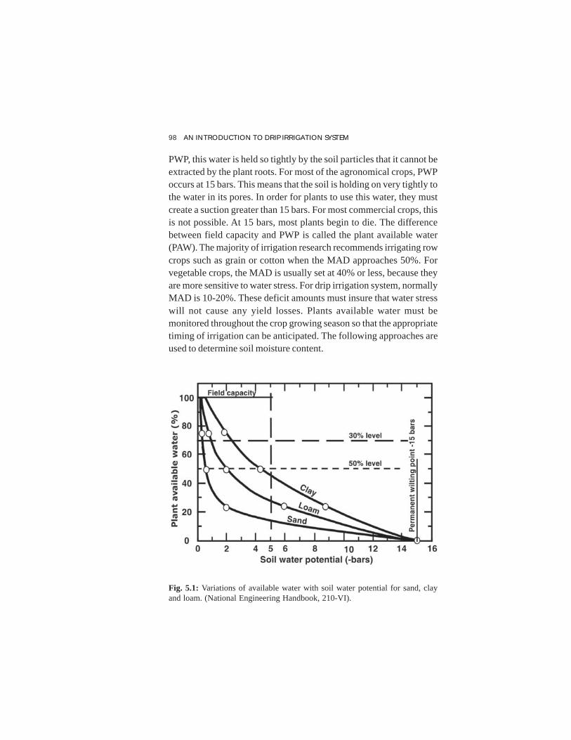
98 AN INTRODUCTION TO DRIP IRRIGATION SYSTEM
PWP, this water is held so tightly by the soil particles that it cannot beextracted by the plant roots. For most of the agronomical crops, PWPoccurs at 15 bars. This means that the soil is holding on very tightly tothe water in its pores. In order for plants to use this water, they mustcreate a suction greater than 15 bars. For most commercial crops, thisis not possible. At 15 bars, most plants begin to die. The differencebetween field capacity and PWP is called the plant available water(PAW). The majority of irrigation research recommends irrigating rowcrops such as grain or cotton when the MAD approaches 50%. Forvegetable crops, the MAD is usually set at 40% or less, because theyare more sensitive to water stress. For drip irrigation system, normallyMAD is 10-20%. These deficit amounts must insure that water stresswill not cause any yield losses. Plants available water must bemonitored throughout the crop growing season so that the appropriatetiming of irrigation can be anticipated. The following approaches areused to determine soil moisture content.
Fig. 5.1: Variations of available water with soil water potential for sand, clayand loam. (National Engineering Handbook, 210-VI).

IRRIGATION SCHEDULING 99
5.2.2.1. Neutron probe
This is a device used to measure the amount of moisture present in thesoil. A neutron probe contains Americium-241 and Beryllium-9. Thealpha particles are emitted by the decay of the americium and collidewith the light beryllium nuclei, thereby, producing fast neutrons witha spectrum of energies ranging up to 11 mega electron volt. Whenthese fast neutrons hit the hydrogen atom present in the soil, they losetheir energy and slow down. Hydrogen atoms have the property ofslowing down the speed of fast moving neutrons. A detector within theprobe measures the rate of fast neutrons leaving and slow neutronsreturning. The detection of slow neutrons returning to the probe allowsan estimate of the amount of hydrogen present. Since water containstwo atoms of hydrogen per molecule, this therefore gives a measure ofsoil moisture.
The major components of neutron probe are a probe, probe carrier,rate scaler and connecting cables (Fig.5.2). When the probe is lowereddown through the access tube at pre-determined depth, fast neutronsemit in the soil which collides with the hydrogen atoms present in thesoil moisture and it gets scattered. The density of scatter cloud of fastmoving neutrons is a function of soil moisture content. This cloud issensed by the sensor in the probe and electrical pulse is transmitted tothe rate scaler connected through the cable. The rate scaler displaysthe pulses in terms of counts per second. These counts per second areconverted into volumetric soil water content. As we know that some ofthe elements available in the soil have the scattering properties forfast moving neutrons, their impact can not be ignored. Therefore, beforeusing neutron probe, it is essential to calibrate the neutron probe. Itaccurately determines the soil moisture and is not affected by thetemperature, soil types and pH. As neutron probe is very costlyinstruments and need to have a licensed operator, this is usually boughtby large organizations or research institutions. Soil moisture contentusing neutron probe is calculated as:
........................................................... (5.6)

100
AN
INT
RO
DU
CT
ION
TO
DR
IP IRR
IGA
TIO
N SY
STEM
Fig. 5.2: Diagram of a neutron probe inserted in the ground (Martin, 2009)

IRRIGATION SCHEDULING 101
where,
MV = Volumetric moisture content, cm
RS = Observed counts/minute in soil
RSTD
= Standard counts/minute in the field
b & j are calibration factors which are calibrated by plotting a graphbetween count ratio and moisture content in soil determined bygravimetric method in the field.
Example 5.1. Determine the soil moisture content using the neutronprobe data as given below:
RS = 4500 counts/min
Rstd
= 6000 counts/min
b = 0.35
j = 0.0
Applying the Eq. 5.6 we get
5.2.2.2. Electrical Resistance
Another method that has been used for several years to determine soilmoisture content is electrical resistance. Devices such as gypsum blocksand Watermark sensors use electrical resistance to measure soilmoisture. The principle behind these devices is that moisture contentcan be determined by the resistance between two electrodes embeddedin the soil. The electrical resistances increase with decrease in soilmoisture content. To measure soil moisture, the porous blockscontaining electrodes are buried in the ground at the desired depth,with wire leads to the soil surface. Wheatstone electrical bridge isused to measure the high values of electrical resistance. The instrumentcan work for a wide range of soil moisture. A meter is connected to thewire leads and a reading is taken (Fig. 5.3). As the soil moisture

102A
N IN
TR
OD
UC
TIO
N T
O D
RIP IR
RIG
AT
ION
SYST
EM
Fig. 5.3: Three resistance blocks anchored by a stake in the field (Martin, 2009).

IRRIGATION SCHEDULING 103
changes, the water content of the porous block also increases ordecrease and this change influences the electrical conductivity. Higherwater content leads to higher conductivity or lower electrical resistance.The relationship between electrical resistance and soil moisture isquantified by a calibration process. This method is not suitable forsoils with freezing temperatures and high salinity.
5.2.2.3. Soil Tension
When the soil dries out, the soil particles retain the water with greaterforce. Tensiometers measure how tightly the soil water is being held.Most tensiometers have a porous or ceramic tip connected to a watercolumn. The tensiometers are installed to the desired depth (Fig. 5.4).As the soil dries, it begins to pull the water out of the water columnthrough the ceramic cup, causing suction on the water column. Thisforce is then measured with a suction gauge connected through a tubeto porous cup. When the tensiometers are installed in the soil, the waterin the porous cup reaches equilibrium with the moisture content in thesurrounding soil. As the soil moisture decreases, the soil dries and thewater begins to flow out of the cup. The vacuum created in the cup bythis suction of water is recorded on the pressure or suction gauge. Inshort, the changes in the soil tension reflect the changes in the soilmoisture surrounding the cup. Some newer models have replaced thesuction gauge with an electronic transducer. These electronic devicesare usually more sensitive than the gauges. Tensiometers work well insoils with high soil-water content, but tend to lose good soil contactwhen the soil becomes too dry. The instruments also suffer from time-lag in response to changes in soil moisture.
5.2.2.4. Time-Domain Reflectometry (TDR)
The TDR instruments work on the principle that the presence of waterin the soil affects the speed of an electromagnetic wave. It slows thespeed of electromagnetic wave. The TDR sends an electromagneticwave through a guide placed into the ground at the desired depth. Itthen measures the time it takes the wave to travel down the guide andreflect back to the guide. The time is recorded and converted to soilmoisture reading. The wetter the soil, the longer it takes for the

104 AN INTRODUCTION TO DRIP IRRIGATION SYSTEM
Fig.5.4: A tensiometer in the field (Martin, 2009).

106 AN INTRODUCTION TO DRIP IRRIGATION SYSTEM
and involvement of high cost. The time domain reflectometry (TDR)method involves measuring the propagation of an electromagnetic pulsealong the wave guides. By measuring the travel time and the velocity,the apparent dielectric constant of the soil can be estimated. Usually,the TDR method is not soil-specific and therefore no soil calibration isrequired and TDR measurements may be affected by soil salinity, soiltemperature, clay type and clay content. The TDR technique mayoverestimate soil-water content in saline soils because the apparentdielectric constant also depends on the electrical conductivity of thesoil. The frequency-domain reflectometer (FDR) method makes useof radio frequencies and the electrical capacitance of a capacitor, formedby using the soil and embedded rods as a dielectric, for determiningthe dielectric constant and thus the soil water content. The signalreflected by soil combines with the generated signal to form a standingwave with amplitude that is a measure of the soil-water content. In thecase of capacitance-type sensors, such as that used by Grooves andRose (2004), the charge time of a capacitor is used to determine thesoil-water content. Profile-probe versions using FDR and capacitancemethods are now commercially available. The FDRs use an ACoscillator to form a tuned circuit with the soil. After inserting probesthat are either parallel spikes or metal rings into the soil, a tuned circuitfrequency is established. This frequency changes depending on thesoil moisture content. Most models use an access tube installed in theground. They read only a small volume of soil surrounding the probes.FDR is also sensitive to air gaps between the access tube and the soil.Many of these newer instruments require installation by professionalsto operate properly.
5.2.2.6. Infrared/Canopy Temperature
Plant indicators are also useful in determining the timing of irrigation.Observing few plants characteristic can give you a good idea of thestatus of the field’s moisture content. An infrared (IR) thermometermeasures the thermal temperature of the plant leaves or a crop canopy.As we know that plants transpire through openings called stomata,once the plants go into water stress, they begin to close their stomataand cease to transpire, causing the plant to heat up and the canopy

IRRIGATION SCHEDULING 107
temperature to rise. Infrared readings can detect this increase in planttemperature. In this method, baseline temperatures need to be takenprior to measurements. The baseline temperature should be taken in awell-watered field, free of water stress. On days when the airtemperature is very high, some plants will stop transpiring for a briefperiod. If infrared readings are being taken at that time, they may readthat there is a water stress when, in fact, it is just a normal shutdownperiod. Compare field readings with your well-watered readings tomake your decision. IR also requires taking temperature readings onclear days at solar noon. This normally occurs between noon and 2:00p.m. This is to assure that the measurement you are taking is atmaximum solar intensity. During the monsoon season, this may bedifficult to achieve due to cloud cover. Early in the season, IR readingswill often measure soil temperature when canopy cover is sparse. Thesereadings usually result in higher temperature readings since the soiltends to heat up quickly. Fig. 5.5 is a diagram of a hand-held IR gun.
5.2.3. Wetting Front Detector
At present numerous methods and devices are available for schedulingof irrigation. These include either physical measurement of the soilwater content by means of e.g. tensiometers and neutron probes, orsimulation models using data from automatic weather stations and cropgrowth parameters. However, in practice it is found that irrigationscheduling is not widely applied mainly because methods are not alwaysuser-friendly and farmers have insufficient knowledge of schedulingtools. Dr. Richard John Stirzaker, a Scientist at CSIRO, Division ofLand and Water, Australia developed a wetting front detector whichalso received the prestigious WatSave Technology Award in 2003 givenby the International Commission on Irrigation and Drainage (Fig. 5.6).
The Wetting Front Detector is made of a funnel, a filter and a float,buried in the root zone. The detector works on the principle of flowline convergence. Irrigation water or rain moving downwards throughthe soil is concentrated when the water molecules enter the wide endof the funnel. The soil in the funnel becomes wetter as the funnelnarrows and the funnel shape has been designed so that the soil at itsbase reaches saturation. Once saturation has occurred, free water flows

108 AN INTRODUCTION TO DRIP IRRIGATION SYSTEM
Fig. 5.6: Dr. Richard John Stirzaker holding the wetting front detector
Fig. 5.5: Hand-held infrared sensor (Martin, 2009)

IRR
IGA
TIO
N SC
HED
ULIN
G109Fig. 5.7: Wetting front detector installed at different depth.

110 AN INTRODUCTION TO DRIP IRRIGATION SYSTEM
through a filter into a small reservoir and activates a float (Fig. 5.7). Itgives a visual signal when the wetting front reaches the required soildepth. The wetting front detector can be used to schedule irrigationbecause the time it takes for water to reach a certain depth depends onthe initial water content of the particular soil. If the soil is dry beforeirrigation the wetting front moves slowly because the water must fillthe soil pores on its way down. Therefore a lot of water is neededbefore the detector will respond. Free water produced at the base ofthe funnel by convergence activates the float in the detector. Water iswithdrawn from the funnel by capillary action after the wetting frontdissipates.

6Hydraulics of Water Flow in Pipes
The designing of any irrigation systems involves the determination ofpipe sizes and uniformity of application of water in the field. Thechannel width of conventional irrigation systems is ensured to carrythe necessary water required for irrigation. It includes all the lossese.g. percolation losses, evaporation losses and leaching of water beyondroot zone. Drip irrigation system also involves determination of pipesizes to carry the desired amount of water. The amount of water to becarried depends upon the type of crop and climatic conditions of theregion. Drip irrigation system is a network of pipes of various sizes;therefore, water flowing through pipe and its basic hydraulic isnecessary to understand first.
6.1. Flow in a Pipe
The cross sectional area of pipe is determined by
….............................................................. (6.1)
where, A is the internal cross sectional area of the pipe, R is internalradius of pipe and D is internal diameter of the pipe line. The rate ofwater flow in a pipe can be given as
Q = A × V…............................................................................... (6.2)

112 AN INTRODUCTION TO DRIP IRRIGATION SYSTEM
where, Q is rate of flow of water (m3/s or cm3/s),
A
is cross sectionalarea of pipe (m2 or cm2) and V is velocity of flow of water (m/s or cm/s).
The velocity of flow of water in a pipe is given as below:
tLV = ….............................................................................. (6.3)
Where, L is the length of the pipe in which water flows and t is time.
Example 6.1. A drip irrigation system was installed in a bananaorchard. A mainline of 63 mm was installed from A to C and sub-mainline of diameter 50mm was taken out from point B. If the velocity offlowing water between A to B is 1.2 m/s and from B to C is 0.7 m/s,determine rate and velocity of flowing water coming out of B.
Solution.
The cross sectional area of main line A1 = 4
2Dπ = 4
3.6 2
×π = 31.15 cm2

HYDRAULICS OF WATER FLOW IN PIPES 113
The cross sectional area of sub-main line A2 =4
2Dπ =4
52
×π = 19.62 cm2
Since the flowing velocity of water is different for A to B and B to C,we will determine the discharge flowing though it.
For A to B:
Q1 = A
1 × V
1 = 31.15 × 120 = 3738 cm3/s
For B to C:
Q2 = A2 × V2 = 19.62 × 70 = 1373.40 cm3/s
The difference between the discharges Q1 and Q
2 will pass through the
sub-main line, so suppose discharge passing out of sub-main line is Q3
Q3 = Q1 - Q2 = 3738 – 1373.40 = 2364.60 cm3/s
Cross sectional area of sub-main line is already known, therefore,velocity of flowing water through sub-main line is
2
3A
QV = = 60.1960.2364 = 120.64 cm/s = 1.20 m/s
6.2. Water Pressure
Water pressure describes the flow strength of water flowing through apipe or other type of channel. It depends on water flow and more waterflow will create more pressure. Water pressure can be expressed in metersrather than atmosphere or psi. The relationship can be shown as follows.
γPH =
where, H is pressure head (m), P is in atmosphere and γ is specificweight (kg/cm3). This can be clearer with this example.
Example 6.2. What will be the pressure of two atmospheres?
Solution.
It is given that P = 2 atmosphere (atm) and γ for water is 0.001 kg/cm3

114 AN INTRODUCTION TO DRIP IRRIGATION SYSTEM
Therefore, γPH = = 2
0.001= 2000cm = 20m
So 2 atmosphere is 20 m of pressure head.
6.3. Estimation of Total Head
Bernoulli’s principle states that for an inviscid flow, an increase in thefluid speed occurs simultaneously with a decrease in pressure or adecrease in the potential energy of fluid. Bernoulli’s principle is basedon the principle of conservation of energy. This means that, in a steadyflow, the sum of all forms of mechanical energy in a flowing fluid isthe same at all points. This requires that the sum of kinetic energy andpotential energy remain constant. Total head or energy head H can beshown as follows.
g
vh
g
v
g
pzH
22
22
+=++=ρ …............................................ (6.5)
Bernoulli’s equation is based on certain assumptions which are statedbelow.
• Flow is steady
• Density is constant i.e. the fluid is incompressible
• Friction losses are negligible
Bernoulli’s equation ceases to be valid before zero pressure is reached.The above equation uses a linear relationship between flow speedsquared and pressure. The total head of water along the pipeline dependson the difference of elevation, pressure and velocity of water and itremains constant throughout the water body. For any two points alongthe flow, the equation takes the following form.
.................................................(6.6)
where,

HYDRAULICS OF WATER FLOW IN PIPES 115
z = the relative elevation of water, m
= the pressure head of water, m
g
v
2
2
= velocity head of flowing water, m
6.4. Head loss Due to Friction in Plain Pipes
6.4.1. Hazen-William’s formula
This is the most commonly used formula for estimating frictional headloss in a steady pipe flow of various pipe materials. The Hazen-Williams formula gives accurate head loss due to friction for fluidswith kinematic viscosity of approximately 1.1 cSt (1 cSt (centiStokes)= 10-6 m2/s). It can be applied for pipes of 50 mm or larger and velocitiesless than 3 m/s. As the roughness coefficient used in this formula doesnot involve Reynolds number, and hence this gives the direct solutions.Due to its simplicity, Hazen-Williams formula has been extended toinclude plastic drip irrigation pipes even though they are smaller indiameter with lower flow rates than those normally encountered inother irrigation situations. The equation is acceptable for cold waterat 15.6 0C. Formula is given below:
( )100
..10212.187.4
852.112 L
D
CQhf ×= ….................................................. (6.7)
where,
hf= frictional head loss in the pipe line, m
Q = discharge in the pipeline, lps
C = friction coefficient to consider pipe material
L = length of the pipeline, m
D = inside diameter of the pipe line, mm.
Manufacturers of pipes for drip irrigation recommended a C value of150 for the plastic pipe and tubing. However, Watters and Keller (1978)

116 AN INTRODUCTION TO DRIP IRRIGATION SYSTEM
showed that C =150 underestimates the pipe friction losses for theflow normally encountered in drip irrigation systems. Howell and Hiler(1974) suggested that C =130 be used for plastic pipes having diameterless than 16mm. Howell et al. (1982) suggested that the best valuesfor drip irrigation systems are C =130 for 14-15mm pipe diameter,C =140 for 19-20 mm, and C =150 for 25-27 mm.
6.4.2. Darcy- Weisbach’s Formula
This is a dimensionally homogeneous formula, which is used forestimating head or pressure loss due to friction along a given length ofpipe. The Darcy–Weisbach equation contains a dimensionless frictionfactor, known as the Darcy friction factor. This is also called the Darcy–Weisbach friction factor or Moody friction factor. The Moody diagramshows the relationship between the relative roughness of the pipe andthe Darcy-Weisbach friction factor (f) for different values of Reynoldsnumber (R
n). The Darcy-Weisbach formula which relates the frication
factor (f) to the head loss in pipes due to friction is given as below.
g
V
D
Lfh f 2
..2
= …................................................................... (6.8)
where,
hf = head loss due to friction, m
L = length of the pipe, m
D = internal diameter of the pipe, mm
V = average velocity of the fluid flow, m/s
g = acceleration due to gravity, 9.81 m/s2
f = a dimensionless coefficient called the Darcy friction factor
Blasius equation for smooth pipes has been recognized as an accuratepredictor of friction factor for plain small diameter plastic pipe.However, in drip irrigation laterals with inserted emitters, the flowregime becomes semi-smooth due to the presence of emitter protrusions(Amin, 1990). Depending upon the flow conditions, the Darcy-Weisbach friction factor (f) can be calculated as fallows;

HYDRAULICS OF WATER FLOW IN PIPES 117
(a) For laminar flow (Rn< 2000) where pipe roughness is not a factor
nRf 64= ….......................................................................... (6.9)
(b) For turbulent flow (4000 < Rn < 105) in hydraulically smooth pipe
such as glass, copper and plastic tubing, the Blasius equation can beused
25.03164.0
nRf = …............................................................... (6.10)
where, Rn is the Reynolds number. Howell and Barinas (1980)
expressed Hazen-Williams formula in a form of Darcy-Weisbachequation to identify friction factor (f) as a function of roughnesscoefficient (C). A reference temperature of 15.60C was used and thefollowing expression was obtained:
148.018.0852.1
1862
nRDCf = ................................................................ (6.11)
where, D is in mm.
6.4.3. Watters and Keller Formula
In an experiment conducted by Watters and Keller (1978), it wasdemonstrated that the Darcy- Weisbach formula can be used forestimating frictional head losses in smooth plastic pipes and tubes.They proposed a simplified form of Darcy-Weisbach formula whichincorporates a friction factor estimated from the Blasius equation forsmooth pipes with a water temperature of 200C and kinematic viscosityof 1.0×10⁻⁶ m2/sec.
75.175.4
465.0 QD
Lhf = ….............................................................. (6.12)
where,
hf = pipe friction loss, m
L = pipe length, m

118 AN INTRODUCTION TO DRIP IRRIGATION SYSTEM
D = inside pipe diameter, mm
Q = pipe flow rate, liters/hr
6.5. Head Loss Due to Friction in Multi-Outlet Pipes
The drip irrigation lateral lines and sub-mains are the pipes withmultiple outlets discharging laterally. The flow conditions in such pipesare generally considered as steady, spatially varied with decreasingdischarge. Flow of water through the length of a single outlet (plain)pipe of a given diameter causes more friction loss than does flowthrough a pipe with a number of outlets. This introduces complicationsin estimation of frictional losses in multi-outlet pipes. The estimationof head loss caused by friction in pipelines with multiple outlets requiresa stepwise analysis starting from most downstream outlet, workingupstream and computing head loss caused by friction in each segment.Christiansen (1942) developed a friction factor known as ‘F’ factor,to avoid the cumbersome stepwise analysis. Computing the head lossin a pipe considering the entire discharge to flow through the entirelength and multiplying by factor F allows the head loss through a singlediameter pipeline, with multiple outlets to be estimated. The derivationof factor was based on the following assumptions:
• No outflow at the downstream end of the pipeline.
• All outlets are equally spaced and have equal discharges.
• The distance between the pipe inlet and the first outlet is equalto one full outlet spacing.
• Hydraulic characteristics remain constant along the length ofthe pipeline.
Factor F is a dimensionless factor and a function of the friction formulaused, and the number of outlets along the pipeline. The head loss in apipeline without outlets can be calculated using any of the well-knownfriction formulas such as Darcy-Weisbach, Hazen-Williams, andothers. This is then multiplied by the factor F to calculate the head losscaused by friction in a pipeline with multiple outlets. Christiansen’sequation for computing reduction coefficient ‘F’ for multiple outlet

HYDRAULICS OF WATER FLOW IN PIPES 119
pipelines, where the first outlet is at full spacing from the main line,can be written as.
( )2
5.0
6
1
2
1
1
1
N
b
NbF
−+++
= …............................................ (6.13)
where,
b = velocity or flow exponent in the head loss equation used, and
N = number of outlets in the pipeline.
In many field layouts, the first outlet on a pipeline can not be locatedat a full spacing from the inlet of the pipe. Jensen and Fratini (1957)developed an adjusted factor F which permitted the calculation of thehead loss caused by friction in pipelines with multiple outlets, with thefirst outlet at one-half of outlet spacing from the pipeline inlet. Scaloppi(1988) derived an expression for the adjusted factor F
a. This expression
allows the adjusted factor to be calculated for a pipeline with multipleoutlets and the first outlet at any fraction of spacing (α) from the pipelineinlet. If the first outlet is one-half of outlet spacing from the pipelineinlet, the adjusted factor by Scaloppi (1988) is identical to that byJensen and Fratini (1957). Scaloppi (1988) derived adjusted factor F(α) can be expressed as:
( ) ( )( )α
αα−−−−=
1
1
N
NFF …............................................................. (6.14)
and in the special case where the first outlet is at half of outlet spacingfrom the mainline (α =1/2)
…....................................... (6.15)
For a single diameter pipeline with multiple outlet, factor
F
or theadjusted factor, F (α), allows rapid calculation of head loss caused byfriction. If multi-diameter pipelines are used, the F factors can not beapplied directly to the entire length of the pipeline. For analyticalpurposes, the pipeline is divided into reaches based on pipeline

120 AN INTRODUCTION TO DRIP IRRIGATION SYSTEM
diameter; then again factor cannot be applied directly to any exceptthe most downstream pipe reaches because other reaches of the pipelinewould have outflow at their downstream ends. To resolve this problem,Anwar (1999) proposed a factor G
a to estimate the friction head losses
in multi-outlet pipes or pipelines with outflow at the downstream ends.Factor G
a can be applied to each reach within a multi-diameter pipeline
to estimate the head loss. An adjusted factor Ga allowed for the first
outlet to be at any fraction of outlet spacing from the pipeline inlet.The following assumptions were made in the theoretical developmentof adjusted factor, G
a.
• The outlets are equally spaced and have equal discharge.
• The pipe friction factor remains constant along the length of thepipeline.
• The velocity head can be neglected.
• The increase in pressure past each outlet caused by a decreasein the flow is equal to the head loss caused by turbulenceassociated with each outlet.
• Head loss at the change in pipe diameter is ignored.
Anwar (1999) proposed the following formula to calculate the G(friction correction factor):
( )( )∑
=+
++
=N
k
m
mmNrk
rNG
11 1
1 ...................................................... (6.16)
where,
N = number of outlets along the pipeline
r = ratio of the outflow discharge to the total discharge through theoutlets (r ≥ 0)
k = integer representing the successive segments of the pipeline.
m and n = exponents of the average flow velocity in the pipeline andinternal pipeline diameter respectively
Further, another equation was proposed for aG (adjusted friction

HYDRAULICS OF WATER FLOW IN PIPES 121
correction factor for pipelines with multiple diameter equally spacedoutlets and outflow).
1
1.
−+−+=
xN
xGNGa
……......................................................... (6.17)
In this equation, if the first outlet is located at a full outlet spacingfrom the pipeline inlet i.e. x = 1, then ( ) GG forxa ==1
Example 6.3. In a mango orchard, a 150m long sub-main line of 50mm diameter is serving 30 numbers of laterals. The sub-main line iscarrying a discharge of 1.4 lps. Take C = 140, m = 1.852 and K = 1.22x 10¹². Determine the frictional head loss in the sub-main pipe line byusing Hazen-William’s formula and Watters and Keller formula.
Solution. Hazen-William’s formula can be given as below.
( )100
..10212.187.4
852.112 L
D
CQh f ×=
where,
hf = frictional head loss in the pipe line, m
Q = discharge in the pipeline, lps
C = friction coefficient to consider pipe material
L = length of the pipeline, m
D = inside diameter of the pipe line, mm.
( )1.852
124.87
1.4 140 1501.212 10 . .
50 100fh = ×
= 1.91m
Now, since there are 30 numbers of outlets are being served with thissub-main pipe, hences a correction fator, F, will also be determined asfollows.
122 AN INTRODUCTION TO DRIP IRRIGATION SYSTEM
( )0.5
2
11 1
1 2 6
bF
b N N
−= + +
+
( )( )
0.5
2
1.852 11 1
1.852 1 2 30 6 30F
−= + +
+ ×
= 0.36
Finally, the friction head loss will be hf x F = 1.91 x 0.36 = 0.68m
According to Watters and Keller formula, frictional head loss can becalculated as.
75.175.4
465.0 QD
Lh f =
where,
hf = pipe friction loss, m
L = pipe length, m
D = inside pipe diameter, mm
Q = pipe flow rate, liters/hr
75.175.4
465.0 QD
Lh f =
1.754.75
1500.465 5040
50=
= 1.11 m
After including factor F, it will be 0.40m.

7Planning and Design of Drip
Irrigation Systems
The planning and design of a drip irrigation system is essential to supplythe required amount of irrigation water. The daily water requirementof the plant depends on the water that is taken by the plant from thesoil and the amount of water evaporates from the soil in the immediatevicinity of the root zone in a day. The plant water intake is affected bythe leaf area, stage of growth, climate, soil conditions etc. The waterrequirement and irrigation schedule can be determined from the soilor plant indicators based methods or soil–water budget method, but.The details of methods of potential evapotranspiration and severaltechniques of irrigation scheduling have been eleborated in Chapter4&5. To apply the required amount of water uniformly to all the plantsin the field, it is required to maintain desired hydraulic pressure in thepipe network. The hydraulic design of drip irrigation system includesdetermining the size of laterals, manifolds, sub-main, main pipeline,selection of appropriate emitter discharge and size of pumping unit.Major steps for the design of a drip irrigation system are
i) Collection of general information
ii) Layout of the drip irrigation system
iii) Crop water requirement
iv) Hydraulic design of the system

124 AN INTRODUCTION TO DRIP IRRIGATION SYSTEM
7.1. Collection of General Information
General information on water source, crops to be grown, topographiccondition, type and texture of the soil and climatic data are essentialfor designing a drip irrigation system. The information on type of soilwill help in selection of emitter and its rated discharge rate. Climaticdata are required to estimate the potential evapotransiration if panevaporation data is not available.
7.2. Layout of the Drip Irrigation System
The layout of the drip irrigation system depends upon the length andbreadth of the field and location of source of water. The decision as tonumber and spacing of the laterals is governed by the nature of thecrop. Each row, two rows or more than two rows can be served by onelateral. Normally the sub-main line runs along the slope and lateralsare laid across the slope or along the contour lines of the field.
7.3. Crop Water Requirement
The daily crop water requirement is estimated by using the equation
V = EPAN
× Kp × K
C × A × W
p …................................................... (7.1)
Net volume of water to be applied, Vn = V - R
e × A × W
p …....... (7.2)
where,
V = volume of water required, litres
EPAN
= mean pan evaporation for the month, mm/day
Kc
= crop coefficient
Kp
= pan factor
A = area to be irrigated, m2
Re
= effective rainfall, mm
Wp
= Percentage wetting
The crop coefficient (Kc) varies with the crop growth stage and season.
It is considered for crop productive stage for the design of a dripirrigation system. . The details have been discussed in preceedingchapter.

PLANNING AND DESIGN OF DRIP IRRIGATION SYSTEMS 125
7.4. Hydraulic Design of Drip Irrigation System
Flow in drip irrigation line is hydraulically steady, spatially variedpipe flow with decreasing discharge. The total discharge in lateral,sub-main or main is decreasing with respect to the length of the line.The lateral and the sub-main lines are having similar hydraulicscharacteristics while the main line is designed based on input pressure,the required pressure and slope of the energy gradient line which willgive a total energy higher than that of required at any sub-main forirrigation. The ideal drip irrigation system is one in which all emittersdeliver the same volume of water in a given time. Under field conditions,it is difficult to achieve this goal; however, the emitter flow variationin the lateral line can be controlled by the hydraulic design. The pipesused in drip irrigation system are made of plastics and are consideredsmooth. The pressure drop due to friction or frictional head loss can beevaluated with the help of the Darcy-Weisbach equation or Hazen-Williams empirical equation. The details of these equations are givenin Chapter 6.
Flow carried by each lateral line (Q1) = Discharge of one emitter ×
No. of emitters per lateral
Flow carried by each sub-main line (Qs) = Q
1 × No. of lateral lines per
sub-main
Flow carried by main line (Q) = Qs × No. of sub-main lines
The diameter of the main, sub-mains and laterals are chosen based onthe hydraulics of pipe flow. The sizes of main, sub-mains, laterals andsize of pumps are estimated using the procedure stated below:
Total head loss due to friction (Hf)
= friction head loss in mains + friction head loss in sub-mains + frictionhead loss in laterals + friction head loss in accessories and fittings
Operating pressure head required at the dripper =He
Total static head = Hs
Total pumping head (H) = Hf + H
e + H
s

126 AN INTRODUCTION TO DRIP IRRIGATION SYSTEM
7.4.1. Development in Design of lateral pipe
Proper design of drip irrigation system consists in assuring a highuniformity of water application. The lateral lines are the pipes on whichthe emitters are inserted. They receive the water from sub-main lineand are usually made of LLDPE ranging in diameter from 12 to 20mm.The emitter discharge is a function of the lateral pressure. Lowdischarges and low pressure heads in the distribution network allowusing of smaller pipes of lower pressure rating which reduces the costs.Since application of water is slow and spreads over a long time, peakdischarges are reduced, thus requiring smaller size pipes and pumpswhich causes less wear and longer life of network. The irregularity ofemitter discharge is essentially due to the pressure variation in laterals,the land slope, and emitter’s characteristics. The discharge of an emitteris also influenced by the water temperature and partial or completeplugging of emitters. When the pipe network is installed, it is difficultto change its design and layout of the system. So, it is essential toassure precision of calculations of frictional losses and pipe sizes.
The design of drip irrigation lateral has been the subject of severalstudies which has been published in peer reviewed journals. We havetried to incorporate the various methods used in designing of laterals.If we go back, it was the graphical methods or polyplot, used byChristiansen (1942). This method got obsolete due to availability ofcomputers and Wu and Gitlin (1974) developed a computer modelbased on the average discharge. Keller and Karmeli (1974) formulateda computational model to calculate the pressure at any point alonglateral by testing many values of emitter’s exponent. Computationsare considerably simplified by assuming that the emitter discharge isconstant along the lateral. Mathematical models have been establishedusing the law of continuity and conservation of energy. Perolt (1977)used an iterative process based on the back step method to convergethe solution. Solomon and Keller (1978) tried the calculation based onthe piezometric curve. In order to increase the efficiency of design,researchers became interested in the hydraulic analysis of drip irrigationlateral. The finite element method (FEM) is a systematic numericalprocedure that has been used to analyze the hydraulics of the lateralpipe network. A finite element computer model was developed by Bralts

PLANNING AND DESIGN OF DRIP IRRIGATION SYSTEMS 127
and Segerlind (1985) to analyze micro-irrigation sub-main units. Theadvantage of their technique included minimal computer storage andapplication to a large micro irrigation network. Bralts and Edwards(1986) used a graphical technique for field evaluation of micro-irrigation sub-main units and compared the results with calculated data.Yitayew and Warrick (1988) presented an alternative treatmentincluding a spatially variable discharge function as part of the basicsolution to drip irrigation lateral design. They expounded twoevaluations: an analytical solution, and a Runge-Kutta numericalsolution of non-linear differential equations.
Drip irrigation system design was further analyzed using themicrocomputer program by Bralts et al. (1991). This program providedthe pressure head and flows at each emitter in the system. The programalso gave several useful statistics and provided an evaluation ofhydraulic design based upon simple statistics and economics criteria.Since the number of laterals in such a system is large, Bralts et al.(1993) proposed a technique for incorporating a virtual node structure,combining multiple emitters and lateral lines into virtual nodes. Afterdeveloping these nodal equations, the FEM technique was used tonumerically solve nodal pressure heads at all emitters. Thissimplification of the node number reduced the number of equationsand was easy to calculate with a personal computer. Most numericalmethods for analyzing drip irrigation systems utilize the back stepprocedure, an iterative technique to solve for flow rates and pressureheads in a lateral line based on an assumed pressure at the end of theline. A drip irrigation network program needs large computer memory,and a long computer calculation time due to the large matrix equations.A mathematical model was also developed for a microcomputer byHills and Povoa (1993) analyzing hydraulic characteristics of flow ina drip irrigation system. Bralts et al. (1993) used the finite elementmethod for numerical solution of non-linear second order differentialequations. Their articles provide a detailed description of other methods.Kang and Nishiyama (1994, 1996) also used the finite element methodto analyse the pressure head and discharge distribution along lateraland sub-main pipe. The golden section search was applied to find the

128 AN INTRODUCTION TO DRIP IRRIGATION SYSTEM
operating pressure heads of lateral corresponding to the requireduniformity of water application. Valiantzas (1998) introduced a simpleequation for direct calculation of lateral hydraulics. Computations arebased on the assumption of a no uniform emitter outflow profile.Lakhdar and Dalila (2006) presented a computer model based uponthe back step procedure and the control volume method tosimultaneously solve non-linear algebraic equations. An alternativeiteration process was developed which simplified the model to designlateral of drip irrigation system.
7.4.1.1. Hydraulic Analysis of Laterals
Hydraulic analysis of drip irrigation laterals is based on the hydraulicsof pipelines with multiple outlets. The successful design is a compromisebetween the choice of high uniformity and low installation cost. It isimportant to calculate the pressure distribution and emitter dischargecorrectly along the lateral. Using equations of energy and massconservation, the closing between two sections of an elementary controlvolume ends up in a two non-linear partial differential equations system,associating pressure and velocity. These equations describe the flowin the lateral; their solution is tedious because of interdependence ofthe discharge and the pressure in a linear relation. The solution ofthese equations cannot be completely analytic due to the empiric relationof discharge emitters and the energy loss relations. Numericalapproaches solve the problem either backward or forward and cantake into consideration the variability in discharge, pressure, diameter,and spacing. Numerical approaches became popular with thedevelopment of personal computers. These approaches to solve thehydraulics of drip systems included the use of finite element methods.Solving the hydraulics of drip irrigation lateral pipelines requiressolving sets of non-linear equations which are common in the hydraulicsof pipe networks.
There are two main approaches in solving these systems of equations.The first approach is a successive linear approximation method in whichthese equations are linearised using an initial solution. This results inconverting the system of non-linear equations into a set of linear

PLANNING AND DESIGN OF DRIP IRRIGATION SYSTEMS 129
equations. Solving such set of linear equations is quite common in thefinite element method where symmetric banded matrices are solvedefficiently. The results are used as an improved estimate of an initialsolution; then a new system of linear equations is formed and solvedagain. The procedure is continued until convergence. The successivelinear approximation approach was implemented to solve the hydraulicsof drip irrigation systems (Hathoot et al., 1993; Bralts and Segerlind,1985; Kang and Nishiyama, 1996a, 1996b). The second approach isto use the Newton-Raphson method to solve the system of non-linearequations. This method showed a speed of convergence much fasterthan successive linear approximation where the two methods startedfrom the same initial solution in analyzing a set of small hypotheticaldrip irrigation systems (Mizyed, 1997). However, the biggestdisadvantage of applying both successive linear approximation andNewton-Raphson methods to drip irrigation systems is requirementsof memory. This resulted when all the laterals and outlets in a real sizedrip irrigation systems were considered.
Besides Finite Element Method and the Newton-Raphson method tosolve the sets of linear equations, control volume method and methodof Runge-Kutta of order four have also been applied in drip irrigationlateral design. The numeric control volume method (CVM) is oftenused to determine pressure and discharge in drip irrigation lateral. It isapplied to an elementary control volume on the lateral and permits aniterative development, volume after volume, from a lateral extremityto the other. Howell and Hiler (1974) and Helmi et al. (1993) appliedthis technique to an example of drip irrigation lateral, starting iterativeprocedure of calculation from the lateral entrance. Thus knowing theoutput discharge to the lateral entrance, represented by the sum ofaverage emitters discharge, the trial and error method is successivelyused till the lateral end, in order to lead to the convergence. However,the risk of obtaining a negative velocity still exists. This approachseems to provide some precise results but could become slow fornumerous reasons of the possible iteration, without excluding thedivergence risk. Another method to solve the set of non-linear equationsis the numeric method of Runge-Kutta of order four. The Runge-Kuttamethod allows the integration of the differential equations system of
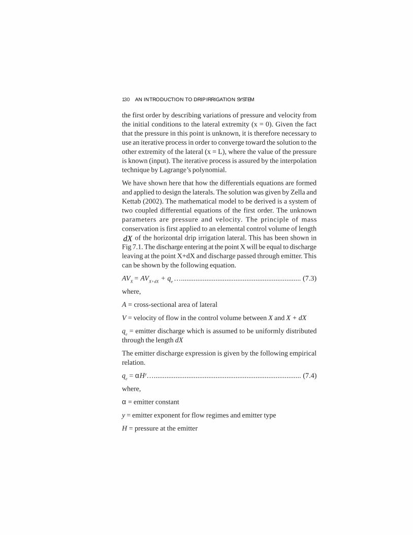
130 AN INTRODUCTION TO DRIP IRRIGATION SYSTEM
the first order by describing variations of pressure and velocity fromthe initial conditions to the lateral extremity (x = 0). Given the factthat the pressure in this point is unknown, it is therefore necessary touse an iterative process in order to converge toward the solution to theother extremity of the lateral (x = L), where the value of the pressureis known (input). The iterative process is assured by the interpolationtechnique by Lagrange’s polynomial.
We have shown here that how the differentials equations are formedand applied to design the laterals. The solution was given by Zella andKettab (2002). The mathematical model to be derived is a system oftwo coupled differential equations of the first order. The unknownparameters are pressure and velocity. The principle of massconservation is first applied to an elemental control volume of length
dX of the horizontal drip irrigation lateral. This has been shown inFig 7.1. The discharge entering at the point X will be equal to dischargeleaving at the point X+dX and discharge passed through emitter. Thiscan be shown by the following equation.
AVX
= AVX+dX
+ qe ….................................................................. (7.3)
where,
A = cross-sectional area of lateral
V = velocity of flow in the control volume between X and X + dX
qe = emitter discharge which is assumed to be uniformly distributed
through the length dX
The emitter discharge expression is given by the following empiricalrelation.
qe = αHy…................................................................................. (7.4)
where,
α = emitter constant
y = emitter exponent for flow regimes and emitter type
H = pressure at the emitter

PLANNING AND DESIGN OF DRIP IRRIGATION SYSTEMS 131
The Bernoulli’s equation can be applied to the flowing fluids. Theprinciple of energy conservation is applied to the elemental controlvolume to give the Bernoulli’s equation in the following form:
hfVg
HVg
H dXXdXXXX ++=+ ++22
2
1
2
1…................................. (7.5)
where,
hf = head loss due to friction between X and X + dX. Its expression canbe given in the following form:
hf = aVm dX…........................................................................... (7.6)
The Reynold’s number is a dimensionless number that gives a measureof the ratio of inertial forces to viscous forces and quantifies the relativeimportance of these two types of forces for given flow conditions.Regime flow is determined by Reynold’s number which can beexpressed by the following equation:
Fig. 7.1: Elemental control volume under consideration

132 AN INTRODUCTION TO DRIP IRRIGATION SYSTEM
µVD
Re = …................................................................................. (7.7)
where,
D = lateral diameter
µ = kinematic viscosity
When Re >2300, m = 1.852 and the value of a in Eq.7.6 is given by the
following equation using the Hazen-Williams formulation.
5835.0AC
Ka
m= …............................................................................. (7.8)
where,
C = Hazen-Williams coefficient
K = coefficient
m = exponent describing flow regime. When Re < 2300; m = 1 and the
value of a is
2
32
gDa
µ= ….............................................................................. (7.9)
where,
g = gravitational acceleration. After expansion of the terms
dXXH + and dXXV + , Eq.7.5 is written as
hfdXx
VdX
x
VVV
gdX
x
HHV
gH XX
XXX
XXX +
∂∂+
∂∂++
∂∂+=+
222 2
2
1
2
1….(7.10)
If the term 2
∂∂
dXx
VX is supposed to be negligible and rearranging the
Eq.7.10, we get
0=+∂∂+
∂∂
hfdXx
V
g
VdX
x
H ….................................................. (7.11)
By using the expansion of VX+dX
in Eq. 7.3, we get

PLANNING AND DESIGN OF DRIP IRRIGATION SYSTEMS 133
0=+∂∂
eqdXx
VA ….................................................................. (7.12)
Finally, by combining Eqs. 7.4, 7.6, 7.9 and 7.10, the final system ofequations are found as
y
X
HAdx
V α−=∂∂
…..................................................................…(7.13)
and
…...................................................... (7.14)
In order to solve the solution of Eqs. 7.13 and 7.14, the velocity at theend of the lateral (V(x=L) =0) and the pressure head (H(x=0) = H
max) are
given. These can be integrated by using the method of Runge-Kutta oforder 4 by constructing an iteration process. Let us assume that H
(L) =
Hmin
is known. A new space variable X is defined such as X = L - X.The system of Eqs. 7.13 and 7.14 becomes
….................................................................... (7.15)
…................................................ (7.16)
The initial conditions to this problem are V(x=L)
=0 and (H(x=0)
= Hmax
).
Iteration Process
To integrate simultaneously Eqs. 7.15 and 7.16, we have to provideonly two estimates of the pressure head at the downstream end of thelateral (X = 0); this can be written as H0
min and H1
min. Now, two solutions
of the initial value problem (7.15) and (7.16) are carried out, yieldingH0
max and H1 max. A new estimate of Hmin can then be obtained by making
use of the interpolating Lagrange polynomial of degree one. This newestimate H
min is written as follows in order to get the next solutionH2
max.


PLANNING AND DESIGN OF DRIP IRRIGATION SYSTEMS 135
iteration process for all the sub-main units. Figure 7.2 shows the totalaverage flow rate of network ( avgQ ) in m3/s, which is an input for thecomputation, the total flow rate TQ in m3/s given after computation,the total pressure head H
T max in m and the velocity V
max in m/s at the
inlet of the network.
Fig. 7.2: An example of drip irrigation network
Fig. 7.3: Lateral pipe of drip irrigation showing elementry control volume
The total network is formed by the identical laterals presented in Fig.7.3. In Fig. 7.3, H
L max represents the pressure at the lateral entrance,
Qmax
represents the total flow rate at inlet of lateral pipe, Vmax
the velocityat lateral pipe entrance, H
L min the pressure at the end of lateral pipe, V
L
minthe velocity at the end of lateral pipe, iqQ = , the discharge of last
emitter and LL
the length of lateral pipe. For the elementary controlvolume (Fig.7.4), the principles of mass and energy conservation areapplied. The ith emitter discharge q
i in m3/s was assumed to be uniformly
distributed along the length between emitters, ∆xL, and is given by:

136 AN INTRODUCTION TO DRIP IRRIGATION SYSTEM
−
= yi Hq α …............................................................................... (7.20)
ory
iii
HHq
+
= +
21α ….................................................................... (7.21)
where,
α = empirical constant
y = emitter exponent
Hi, H
i+1 = pressure at ith and (i+1)th point
H = average pressure along ∆xL. The mass conservation equation for
the control volume gives:
iii qt
Mt
M += +1 …............................................................... (7.22)
where,
Mi= water mass at the entrance of the control volume, kg
Mi+1
= water mass at the exit control volume, kg
t = time in s.
Fig. 7.4: Elementry control volume

PLANNING AND DESIGN OF DRIP IRRIGATION SYSTEMS 137
The energy conservation between i and i+1 is as follows:
Ei = E
i+1 + ∆H …...................................................................... (7.23)
where,
Ei= flow energy or pressure in at the input
Ei+1= flow energy at the exit
∆Η = local head loss hf due to the emitter in meter to friction along∆xL.
The head losses ∆Η are given by the following formula:
Lm
L xVaH ∆=∆−
….................................................................... (7.24)
L
m
ii xVV
aH ∆
+=∆ +
21 ….............................................................. (7.25)
VL in m/s, is the average velocity between i and (i+1), V
i and V
i+1 are
velocity respectively at thi and (i+1)th cross-section lateral, the valueof parameter α is given by Hazen-William equations:
for turbulent flow, Re is Reynold’s number, R
e > 2300,
5835.0L
m AC
Ka = …...................................................................... (7.26)
for laminar flow, Re < 2300,
2
32
LgDa
ν= …............................................................................... (7.27)
where,
C = Hazen-William coefficient
K = proportional coefficient
m= exponent (m = 1 for laminar flow, m = 1.852 for turbulent flow)
AL = cross-sectional area of lateral pipe, m2
DL = interior lateral pipe diameter in m
v = kinematic viscosity, m2/s
g = gravitational acceleration, m/s2.HL and V
L are respectively the

138 AN INTRODUCTION TO DRIP IRRIGATION SYSTEM
average pressure and the average velocity between ith and (i+1)th emitteron the lateral. The calculation model for lateral pipe solvessimultaneously the system of two coupled and non-linear algebraicequations, having two unknown values: V
i+1 and H
i+1.
Equations (7.22) and (7.23) become:
ALV
i = A
L V
i+1 + q
i …................................................................. (7.28)
xVV
ag
VH
g
VH
m
iii
ii
i ∆
+
++=+ +++ 222
112
1
2
….......................................... (7.29)
and equations (7.28) and (7.29) become:
y
ii
Lii
HH
AVV
+−= +
+ 21
1
α …......................................... (7.30)
( ) xVV
aVVg
HHm
iiiiii ∆
+−−+= +
++ 22
1 11
221 ….................................. (7.31)
For the lateral, equations (7.30) and (7.31) become:
LL
yL
L xA
H
dx
dV
∆−=
−
α ............................................................ …(7.32)
−
−=
m
LL
Vadx
dH…....................................................................... (7.33)
For sub-main pipe, equations system is
SS
S
S xA
Q
dx
dV
∆=
….................................................................... (7.34)
−
−=
m
SS
Vadx
dH …..................................................................... (7.35)
where,
QS= flow rate in sub-main pipe
AS= a cross sectional area of sub-main pipe
VS and H
S, respectively, are velocity and pressure in sub-main pipe. At

PLANNING AND DESIGN OF DRIP IRRIGATION SYSTEMS 139
the end of the lateral Vi = 0, H
L max is given at entrance of lateral pipe,
inlet head pressure. The slop of lateral and sub-main pipe is assumednull. When H
L max is fixed, the computation program of lateral can give
the distribution velocity or emitter’s discharge and pressure alonglateral. Theoretical development giving equations (7.30), (7.31) and(7.32), (7.33) can be solved without the use of matrix algebra throughCVM.
As we know the economics of drip irrigation largely depends uponsize and length of drip irrigation lateral and drip irrigation systemrequires large amount of pipe per unit of land, the pipe cost must beeconomically feasible.Appropriate design saves the cost and ensurereliability of the drip system. Besides, modifying the conventional cropgeometry can also considerably reduce drip irrigation system cost. Theplant to plant and row to row spacing can be changed without changingthe plant population per unit area. The design of drip irrigation lateralis mainly concerned with the selection of the pipe size for a givenlength which can supply the estimated amount of water to the plantskeeping the desired range of uniformity. Drip irrigation lateral designcan be classified into mainly two types of design problems:
1. Lateral length is unknown and pipe size is given;
2. Pipe size is unknown but lateral length is constrained;
Usually pipe sizes are limited to pipe diameter less than 20 mm byeconomics. The information required for designing laterals are fieldslope, emitter flow rate, number of emitters per plants, emitter flowfunction, plant spacing and desired uniformity. In first type of problemthe maximum lateral length is determined while maintaining therequired uniformity value. The allowable energy loss can be determinedusing Fig. 7.5 and the following relationships:
x
n
o
n
o
q
q
P
P/1
= ….......................................................................... (7.36)
x
n
o
e
r
n
oo
q
q
K
q
P
PP
/1
)2()(
−××
= γ ….................................................. (7.37)

140 AN INTRODUCTION TO DRIP IRRIGATION SYSTEM
γn
n
PH = ; γ
oo
PH = …............................................................. (7.38)
LSHHH oon +−=∆ ................................................................. (7.39)
0.65
0.35 1.711.70100
e
r
C SL H D
q
= ∆
…............................................................ (7.40)
where,
Pn = pressure at the head of the lateral, kPa
Po = pressure at the end of the lateral, kPa
qn = q
o emitter flow rate at the head and end of the lateral respectively,
lph
γ = specific weight of water, 9.81 kN/m3
Hn = H
o pressure head at the inlet and outlet of the lateral respectively, m
∆Η = pipe friction energy loss, m
D = inside pipe diameter, mm
Se = emitter spacing, m
C = Hazen-Williams roughness coefficient
So = field slope (positive for down and negative for up)
L = lateral length, m
Ke = proportionality factor that characterizes the emitter dimensions
For the second type of problem the following formula can be used forcalculating pipe diameter.
1.852
0.20 0.58 1000.73 ( ) ( ) r
e
qD H L
C S−
= ∆
….......................................... (7.41)
When water is removed through drippers along the laterals, the frictionloss for the given diameter and length of lateral will be less than if theflow was constant for the entire length. A reduction factor (F) is multipliedwith the estimated frictional loss which can be estimated by

PLANNING AND DESIGN OF DRIP IRRIGATION SYSTEMS 141
26
1
2
1
1
1
N
m
NmF
−+++
= …............................................................. (7.42)
where,
m = 1.852 for the Hazen-Williams equation and 2 for the Darcy-Weisbach equation, and
N= number of outlets on the lateral.
The values of F for different ‘m’ are given in Table 7.1.The emitterdischarge decreases with respect to the lateral length when the laterallength is laid on zero slope or uphill. When the lateral pipe is laid onmild downhill slopes, the emitter discharge decreases with respect tothe lateral length and reaches a minimum emitter discharge and thenincreases with respect to the length of the lateral line. This is becausethe gain of energy due to the land slope at a downstream section islarger than the energy drop by friction. There is yet another situationwhere the emitter discharge increases with respect to the length of
Fig. 7.5: Relationship between emitter flow variation and uniformity coefficient

142 AN INTRODUCTION TO DRIP IRRIGATION SYSTEM
lateral line. This is caused by steep slopes where the energy gained bythe slopes is larger than friction drop for all section along the lateralline. Use of series of pipe sizes in laterals or submain design will helpto reduce the maximum pressure variation. By changing the pipe sizeit is possible to make the friction drop approach more closely to theenergy gain at all points along the line. The line slope of each sectioncan be used as the energy slope to design the size of the lateral and submains. This can be used for both uniform and non-uniform slopes.
Example 7.1. Determine the length for a 16 mm inside diameter dripirrigation lateral laid out in a row of mango young plants, spaced 6 mapart with 4 emitters supplying water to each plant. The rated dischargecapacity of emitter is 4 lph with emitter flow function q = 2.52 (P/g)0.8. The slope of the field is 1.0 percent and uniformity coefficient of95 % is desired to be achieved.
Solution: As the emitter flow function of is given as q = 0.63 (P / g) 0.8.Therefore, equating it with Eq. 3.5., We get K
e = 2.52 and x = 0.8
Since 4 emitters are being used for one plant, the required emitter flowdischarge is
qr = 4 × 4 = 16 lph
For uniformity coefficient of 95 %, qn/q
o is estimated as 1.2 from Fig.7.5
= 0.86
Table 7.1: Values of F for different numbers of outlets
Number of outlets F
m = 1.85 m = 1.9 F = 2.0
1 1.000 1.000 1.0002 0.639 0.634 0.6253 0.535 0.528 0.5184 0.486 0.480 0.4695 0.457 0.451 0.4406 0.435 0.433 0.421
Contd.

25.1
)2.1
12(
52.2
16)81.9()86.0(
−××=oP
γn
n
PH =
81.9
120

144 AN INTRODUCTION TO DRIP IRRIGATION SYSTEM
γo
o
PH = =
81.9
96 = 9.7 m
Now, it is given that D = 16 mm; Se = 6 m; q = 16 lph; C = 130
Pipe friction energy loss will be determined by using Eq.7.39
∆H = Hn - H
o + S
o L
= 12.2 – 9.7 + (0.01) (L)
= 2.5 + 0.01 L
Now, putting the value of ∆Η in the Eq. 7.40, we get the followingequation to determine the length of the lateral as follows
65.0
71.135.0
16100
6130)16()01.05.2(70.1
××
+= LL
The length of the lateral can be determined by trial and error approachin MS Excel. Calculate all the terms separately and then multiply eachterm and change the value of L. After few trials, L = 208m for a givenpipe size of 16 mm at the desired uniformity coefficient of 95% wasobtained, however this pipe length is too long. By reducing the diameter,pipe length can be reduced.
7.4.2. Design of Sub-main
The sub-main line hydraulics is similar to the principles applied in thedesign of lateral hydraulics. The sub-main hydraulics characteristicscan be computed by assuming the laterals are analogous to emitters onlateral line. Hydraulics characteristics of sub-main and mainline pipeare usually taken hydraulically smooth since PVC and HDPE pipe arenormally used. The Hazen-Williams roughness coefficients (C) rangefrom 130 to 150. The energy loss in the sub-main can be computedwith the methods similar to those used for lateral computations.
7.4.3. Design of Main
Usually the pressure controls or adjustments are provided at the sub-main inlet. Therefore energy losses in the mainline should not affect

PLANNING AND DESIGN OF DRIP IRRIGATION SYSTEMS 145
system uniformity. There is no outlet in case of main line; thereforereduction factor is not multiplied. The frictional head loss in mainpipeline is calculated in the same way using Hazen-Williams, Darcy-Weibach or Watters and Keller’s formula.
7.5. Pump Horse Power Requirement
Total dynamic head (H) is determined by adding all the frictional headlosses through lateral, sub-main and main line, total static head andoperating pressure required at the emitters. The horse power of pumpis estimated by using the estimated dynamic head and pump discharge.
Pump Horse power ( =)hp mp
QH
ηη ×××
75 …...................... (7.43)
where,
H = total dynamic head , m
Q = total discharge through main line, lps
np and n
m = efficiency of pump and motor, respectively
Example 7.2. Design a drip irrigation system for a mango orchard of1 ha area with length and breadth of 100 m each. Mango plants havebeen planted at a spacing of 5 × 5.5 m and the age of crop is 3 years.The maximum pan evaporation during summer is 12 mm/day. The otherrelevant data are given below:
Land slope = 0.40 % upward
Water source = A well located at the S–W corner of the field
Soil texture = Sandy loam
Field capacity(FC) = 16 %
Wilting point (WP) = 8 %
Apparent specific gravity (AS) = 1.4 g/cc
Effective root zone depth (Zr) = 120 cm
Maximum allowable deficit (MAD) = 20%

146 AN INTRODUCTION TO DRIP IRRIGATION SYSTEM
Wetting area percentage (WA) = 30 %
Pan coefficient = 0.7
Crop coefficient = 0.8
Solution
Step 1.
Estimation of Water Requirement
Evapotranspiration of the crop = pan evaporation Pan coefficient Cropcoefficient
= 12 × 0.7 × 0.8
= 6.72 mm/day
Net depth of water application = (FC – WP) x AS x Zr x 10 x PWD xWA
= (16-8) x 1.4 x 1.20 x 10 x 0.20 x 0.30
= 8.06 mm
If the efficiency of the system is 95%, Es = 0.95
Gross depth of water application 8.06
= = 8.48 mm0.95
Step 2.
Emitter Selection and Irrigation Time
Emitters are selected based on the soil moisture movement and croptype. Assuming three emitters of 4 lph, placed on each plant in atriangular pattern are sufficient so as to wet the effective root zone ofthe crop.
Total discharge delivered in one hour = 4 × 3 = 12 lph
Maximum crop evapotranspiration is already known as 6.72 mm/day
Irrigation interval 8.48
= = 1.26 days 30 hrs6.72
≈

PLANNING AND DESIGN OF DRIP IRRIGATION SYSTEMS 147
Application rate of the system = ( )e l
q
S S WA×
= 125.0 5.5 0.30× ×
= 1.45 mm/hr
Duration of water application = Gross depth of water application
Application rate of the system
= 8.48
1.45
= 5.8 hrs
Step 3.
Discharge Through Each Lateral
A well is located at one corner of the field. Sub-main will be laid fromthe centre of field (Fig. 7.6). Therefore, the length of main, sub-main,and lateral will be 50m, 97.25m, 47.5m each respectively. The lateralswill extend on both sides of the sub-main. Each lateral will supplywater to 10 mango plants.
Total number of laterals = (100/5.5) × 2 = 36.36 (Considering only 36)
Discharge carried by each lateral, Qlateral = 10 × 3 × 4 = 120 lph
Total discharge carried by 36 laterals = 120 × 36 = 4320 lph
Each plant is provided with three emitters, therefore total number ofemitters will be 36 × 10 × 3 =1080
Step 4.
Determination of Manifolds
Assuming the pump discharge = 2.5 lps = 9000 lph
Number of laterals that can be operated by each manifold = 9000/120 = 75
So only one manifold or sub-main can supply water to all the lateralsat a time.


PLANNING AND DESIGN OF DRIP IRRIGATION SYSTEMS 149
head loss due to friction is 10% of head of 10 m (head required tooperate 4 lph emitters) is 1m, therefore 12 mm diameter lateral pipesize is selected. You can select 16mm pipe also but the cost will bemore.
Step 6.
Size of Sub-Main
Total discharge through the sub-main = Qlateral × Number of laterals
= 120 × 36
= 4320 lph = 1.2 lps
Assuming the diameter of the sub-main as 50 mm. The values ofparameter of the Hazen- Williams equation are
C = 150, Q = 1.2 lps, D = 50 mm, K = 1.22 × 10¹², F = 0.364
364.050
)150/2.1(1022.1)100(
87.4
852.112 ×××=fh
= 0.31 m
hf for 97.25 m of sub-main pipe length = 0.31 × (97.25/100) = 0.30 m
Therefore, frictional head loss in the sub-main = 0.30 m
Head at the inlet of the sub-main = Hemitter + Hf lateral + Hf submain + Hslope
= 10 + 0.26 + 0.30 + 0.40 = 10.96 m
Pressure head variation = 10096.10
26.1096.10 ×−
= 6.38 %Estimated head loss due to friction in the sub-main is much less thanthe recommended 20% variation, hence reducing the pipe size from50 to 35 mm will probably be a good option.
= 1.75 m
hf for 97.25 m pipe = 1.75 × (97.25/100) = 1.70 m


PLANNING AND DESIGN OF DRIP IRRIGATION SYSTEMS 151
Pump Horse power ( =)hp p
QH
η××
75
where,
H = total dynamic head, m
Q = total discharge through main line, lps
np = efficiency of pump
hp = 60.075
06.242.1
××
= 0.64 ≅ 1.0
Hence 1 hp pump is adequate for operating the drip irrigation systemto irrigate for 1 ha area of citrus crop.
The design details are given as
Operating time of the system = 5.8 hrs
Inrrigation interval = 30 hrs
Length of laterals = 47.5m
Number of laterals = 36
Diameter of lateral = 12mm
Length of sub-main = 97.25m
Number of sub-main = 1
Diameter of sub-main = 35mm
Length of main = 50m
Number of main = 1
Diameter of main = 50mm
Total power required = 1 hp

152 AN INTRODUCTION TO DRIP IRRIGATION SYSTEM
Example 7.3. The field is located in Old Alluvial Zone andcharacterized by moderate cold. The average annual rainfall is 1500mm. Winter season i.e. November to February receives scanty rainfall.The area of the field is 21.45 ha with majority of sandy loam soil. Thefield capacity of the soil is 16% and permanent wilting point is 6%.The infiltration rate of the soil is 14 mm/hr. The planting distance is1.8 m x 0.4 m
Solution
Since planting spacing is 1.8 x 0.4 m
Plant population per ha = 10000 1.8×0.4
= 13889
Effective crop root depth is assumed as 0.60 m. We have crop coefficient(Kc
) values for different growth stage of tomato. The Kc value for highly
evaporative demand period i.e. mid season (70-115 day) will be
Fig. 7.6: Layout of drip irrigation system for 1 ha of Mango orchard


154 AN INTRODUCTION TO DRIP IRRIGATION SYSTEM
( )0.176
0.22 5 100.031 5.92
4
−− ×=
= 0.46 m = 46cm
Therefore, the radius of wetted circle will be 23 cm
We can also estimate the maximum radius of wetted circle with thefollowing expression.
k
qRMAX ×
=π
where, q is cm3/hr and saturated hydraulic conducivity, K, is in cm/hr.
MAXR = 4000
3.14 1.8×
= 26.60 cm
Therefore wetted width = 53.20 cm
Wetted area of one emitter = πRMAX
2
3.14 × (26.60)2
= 2221.73 cm2
= 0.22 m2
Length of the field = 715 m
Width of the field = 300 m
Total number of lateral at a distance of 1.8 m
width of field=
spacing of laterals
300= = 166.66 168 even number
1.80≈
No. of emitters per lateral Length of field
= spacing of emitter
715=
0.4= 1787.5 1788≈

PLANNING AND DESIGN OF DRIP IRRIGATION SYSTEMS 155
Here it is assumed that length of a single lateral is length of field
Total no. of emitters in the field = No. of laterals x no. of emitters/lateral
= 168 x 1788
= 300384
Total wetted area by emitters
= 0.22 x 300384
= 66084.48 m2
= 6.61 ha
Total area of field = 21.45 ha
Percentage wetted area 6.61
= x 100 = 30.81%21.45
Considering a flat percentage wetted area as 35%
Net depth of water application
= (FC – WP) x AS x Zr x 10 x PWD x WA
= (16-6) x 1.4 x 0.80 x 10 x 0.20 x 0.35
= 7.84 mm
If the efficiency of the system is 95%, Es = 0.95
Gross depth of water application 7.84
= = 8.25 mm0.95
Maximum crop evapotranspiration is already known as 6.72 mm/day
Irrigation interval 8.25
= = 1.23 days 30 hrs6.72
≈
Application rate of the system = le SS
q
×
= 8.14.0
4
×
= 5.55 mm/hr

156 AN INTRODUCTION TO DRIP IRRIGATION SYSTEM
Duration of water application = Gross depth of water application/Application rate
= 8.25/5.55
= 1.48 hr
For deciding the number of sub-plots, consider 80% of irrigationinterval it comes 24 hrs.
No. of sub-plots
80% of irrigation interval=
Duration of water application
24= = 16.21 16 sub-plots
1.48≈
Design of Lateral Pipe
Choose lateral pipe of 20 mm diameter
Working pressure = 30 m
Length of one lateral pipe in one sub-plot
715= = 89.37 89.5 m
8≈
No. of drippers on each lateral 89.50
= = 2240.4
Maximum allowable head loss in the main line = 20% of workingpressure
20= 30 x = 6 m
100Discharge flowing through each lateral Q = 4lph x 224
= 0.004 m3/h x 224 = 0.90 m3/h
= 0.25lps
Head loss due to friction along the 89.5m of the lateral line

PLANNING AND DESIGN OF DRIP IRRIGATION SYSTEMS 157
If we consider local heal loss as 10% of loss along the lateral (hf)
ht × 1.10 × F
hf = x 1.10 x F
= 4.76 x 1.10 x 0.366
= 1.92 m
This head loss of lesser than 6 m, so 20 mm will be selected.
Therefore, total pressure required at the inlet of the lateral
= hs + 0.75 x hf
= 30 + 0.75 x 1.92
hfemitter
= 31.43 m
Design of the Manifold
Only one side of the manifold is connected with laterals.
No. of lateral pipes in manifold towards slope
300 / 2= = 83.33 84
1.8≈
Main line is in between the field
Length of manifold 300
= = 150 m2
Elevation difference = 0.50 m
Discharge carried out by one manifold
Q = No. of laterals x Discharge passing throuh one lateral
= 84 x 0.90 = 75.6 m3/h
Select the size of manifold as 140 mm PVC pipe (C=140)

158 AN INTRODUCTION TO DRIP IRRIGATION SYSTEM
Head loss due to fixation
Considering 10% of head loss along the sub-main
Total head loss along the manifold = 0.708 x 1.10 = 0.77 m
Now pressure required at the inter of the manifold
= hfe + 0.75 hf - (Z/2)
= 31.43 + 0.75 x 0.77 - (0.5/2)
hfmanifold
= 31.43 + 0.58 - 0.25 = 31.76 m
Design of Main Line
Total number of manifold = 16
Number of manifold working at a time = 1
Length of main line = 7 x 89.85 = 626.5 m
Here we can go for telescopic design of main line.
First 400 m length is of 225 mm dia and remaining 226.5 m is of 140mm dia.
For 400 m length with 225 mm pipe dia, discharge carried out by thepipe is = 75.6 m3/h
(Since one manifold is operating at a time, main line will carry onlydischarge of one manifold anytime)
Pressure head loss in main line
1.8512
4.87
(21/140) 400hf = 1.22 x 10 x x x 0.366 = 0.18 m
(225) 100
For remaining 226.5 m length of pipe with 140 mm dia

PLANNING AND DESIGN OF DRIP IRRIGATION SYSTEMS 159
1.8512
4.87
(21/140) 226.5hf = 1.22 x 10 x x x 0.366 = 1.07 m
(140) 100
Total head loss along the main line = 0.18 + 1.07 = 1.25 m
Considering 10% loss in the main line
Total frictional head loss hf = 1.25 x 1.10 = 1.38 m
Again considering the elevation difference as 1 m
Total head loss at the inlet of main line
= hfmanifold
+ 0.75 x 1.38 + ½
= 31.76 + 1.04 + 0.5
= 33.32 m
Pump Selection
Considering the head loss in control head is 10% of total head loss
= 33.3 x 1.10 = 36.63 m
Required discharge capacity of the pump = 89.5 m3/h
Required horse power = ofpumpEfficiency
HQ
××
273
= 75.0273
63.365.89
××
= 16 hp
7.6. Design Tips for Drip Irrigation
Though the design methodology has been explained previously, thereare some points which should be considered while planning a dripirrigation system for crop production. As drip systems is also used forfertigation and chemical injection, application uniformity of fertilizersand chemicals will be affected with water application efficiency of thedrip irrigation systems. Here are some points.
• Length of lateral lines should not exceed the recommendedlength. Excessive length of laterals will result in poor uniformity

160 AN INTRODUCTION TO DRIP IRRIGATION SYSTEM
and uneven water application. For better precaution, check theamount of water supplied by the emitters in the last section ofthe lateral.
• The sizes of main and sub-main lines should be properly selectedto avoid excessive pressure losses and velocities. Excessivevelocities of water in the lines, due to too small a diameter, cancreate a water hammer which can damage the main and sub-main lines.
• Use pressure compensating emitters where necessary.
• Choose the irrigation area zone in conformity with the existingwater pump.
• The drip irrigation systems experience clogging of emitters whichreduce water application uniformity. The degree of cloggingdepends on water quality, type of emitters, and quality of waterfiltration. An irrigation system should include an injection portto allow for injection of chlorine for flushing out the systems atregular interval.
• The irrigation system injecting fertilizers or chemicals is requiredto be provided with proper backflow mechanism to prevent thecontamination of the water source.
• Pressure changes in the irrigation line should be monitored. Anincrease in pressure can be caused by emitter clogging or someother blockage such as the failure of a valve or pressure regulator.A pressure drop may indicate a broken line, leaking valves, thefailure of flush valves to close properly.
7.7. Economic Analysis
Investment on installation of drip irrigation system must beeconomically viable and justified. If the project gives economic surplus,we can say the project is economically viable. As drip irrigation involvesconsiderable cost, the economic appraisal of the installation of dripsystem must take full account of all the cost and benefit likely to beaccrued from the crops to be grown and its byproduct. Economic


() ()()1
1
n
n
ePW e PW
i
+ =× +

()()11
1
−++=
n
n
i
iiCRF
()n
t=0
NPV = 1
t tt
B C
i
−+
∑

164 AN INTRODUCTION TO DRIP IRRIGATION SYSTEM
i = discount rate,
n = number of years.
7.7.4.2. Benefit Cost Ratio (BCR)
The discounted measure of the project worth can be expressed bybenefit-cost ratio. This is the ratio implies the return per rupeeinvestment. The benefits and costs of any year are converted into theequivalent basis (i.e. present year) to find out the benefit cost ratio. IfBCR value is bigger than 1, benefit has more than the cost, then theproject is feasible. The B/C ratio can be worked out by using thefollowing formula:
( )
( )∑
∑
=
=
+
+=n
tt
t
n
tt
t
i
Ci
B
BCR
0
0
1
1 ….................................................................. (7.50)
7.7.4.3. Internal Rate of Return (IRR)
The average annual percentage return is expected from a project, wherethe sum of the discounted cash inflows over the life of the project isequal to the sum of the discounted cash outflows. Therefore, the IRRrepresents the discount rate that results in a zero NPV of cash flows.In this method also, we convert all the costs as well as benefits of anyyear into equivalent basis (i.e. present year). IRR can be comparedwith the existing bank interest rate to judge the economic feasibility ofthe project. IRR is calculated from the following principle,
0 0(1 ) (1 )
n nt t
t tt t
B C
i i= =
=+ +∑ ∑ ……....................................................... (7.51)
The cost of the drip irrigation system include all of the fixed costs,operation costs, maintenance costs and all the costs incurred to theproject. The benefit of the investment will include, income fromproduction, any form of by-product, salvage value etc.
Example 7.4. Tomato crop is to be cultivated in 1 ha area under dripirrigation system. Determine the net present value (NPV) and benefit

PLAN
NIN
G A
ND
DESIG
N O
F DR
IP IRR
IGA
TION
SYSTEMS
165
Year Fixed cost Operation and Cash inflow Year Fixed cost Operation and Cash inflowmaintenance maintenance
1. 180000 40000 120000 6 — 50000 1200002. — 40000 120000 7 — 50000 1200003. — 40000 120000 8 — 60000 1200004. — 45000 120000 9 — 60000 1200005. — 45000 120000 10 — 60000 120000

166 AN INTRODUCTION TO DRIP IRRIGATION SYSTEM
cost ratio (BCR). The cash flow pattern is given hereunder and takeinterest rate as 12% and life of the drip system as 10 years. Theoperation cost include the maintenance cost of drip systems and costof cultivation which may increase over the period of time, however thereturn i.e. cash inflow has been assumed constant with a yield of tomatoas 30t/ha.
Solution
First we will calculate the discount rate which is also called the discountfactor with the following formula
Discount factor = ( )
+ ni1
1
here, n is 1, 2, 3, ….10.
Cash outflow = Fixed cost + Operation and maintenance
Cash flow = Cash inflow - Cash outflow
Discounted cash flow = Cash flow x Discount factor
Discounted cash outflow = Cash outflow x Discount factor
Discounted cash inflow = Cash inflow x Discount factor
The result is presented in a tabular form.
Net Present Value (NPV) = Sum of discounted cash flow for the periodsof 10 years
= ` 2,53,960
Since NPV is greater than zero, investment on drip irrigation iseconomically feasible. Now calculate benefit cost ratio (BCR)
outflowcashDiscounted
lowcashDiscountedratiotbenefitDiscounted
infcos =
Discounted benefit cost ratio outflowcashDiscounted
lowcashDiscounted inf=

PLAN
NIN
G A
ND
DESIG
N O
F DR
IP IRR
IGA
TION
SYSTEMS
167
Year Fixed cost Operation and Cash Cash Cash Discount Discounted Discounted Discountedmaintenance outflow inflow flow factor cash flow cash outflow cash inflow
1. 180000 40000 220000 120000 -100000 0.8929 -89290 196438 1071482. 40000 40000 120000 80000 0.7972 63776 31888 956643. 40000 40000 120000 80000 0.7118 56944 28472 854164. 45000 45000 120000 75000 0.6355 47662 28597 762605. 45000 45000 120000 75000 0.5674 42555 25533 680886. 50000 50000 120000 70000 0.5066 35462 25330 607927. 50000 50000 120000 70000 0.4523 31661 22615 542768. 60000 60000 120000 60000 0.4039 24234 24234 484689. 60000 60000 120000 60000 0.3606 21636 21636 43272
10. 60000 60000 120000 60000 0.322 19320 19320 38640
Total 670000 1200000 253960 424063 678024

168 AN INTRODUCTION TO DRIP IRRIGATION SYSTEM
= 424063
678024
= 1.60
Now what will happen to BCR if discounted cash flow technique isnot followed in economic analysis?
Undiscounted cash flow technique = outflowCash
lowCash inf
=670000
1200000
= 1.80
BCR is higher in case of undiscounted cash flow technique which maynot be appropriate techniques of project appraisal and feasibility study.
Example7.5. Determine the internal rate of return of the investmentmade in covering 1 ha Mango (Amprapali) orchard under dripirrigation. The cash flow patterns are given hereunder and take interestrate as 12% and life of the drip system as 10 years. The operation costinclude the maintenance cost of drip systems and cost of cultivationwhich may increase over the period of time, however the return i.e.cash inflow has been assumed constant.
Solution. As in the previous example, we will calculate the discountrate which is also called the discount factor with the following formulafor 12, 14, 18 % of interest rate.
Discount factor = ( )
+ ni1
1 here, n is 1, 2, 3, ….10.
Cash inflow has not been considered for first three years and fromfourth years onwards, we have included cash inflows. Again it hasbeen assumed that cash inflows through out the life cycle as constant,of course it is not true. The result is presented in a tabular form.
As NPV of ` 29189.4 is greater than zero, the investment iseconomically good.

PLAN
NIN
G A
ND
DESIG
N O
F DR
IP IRR
IGA
TION
SYSTEMS
169
Year Fixed cost Operation and Cash inflow Year Fixed cost Operation and Cash inflowmaintenance maintenance
1. 75000 10000 — 6 — 12000 500002. — 10000 — 7 — 12000 500003. — 10000 — 8 — 15000 500004. — 12000 50000 9 — 15000 500005. — 12000 50000 10 — 15000 50000

170A
N IN
TR
OD
UC
TIO
N T
O D
RIP IR
RIG
AT
ION
SYST
EM
Year Fixed cost Operation and Cash outflow Cash inflow Cash flow Discounted cash flowmaintenance
12% 14% 18%1. 75000 10000 85000 0 -85000 -75896.5 -74561.4 -72033.92. 10000 10000 0 -10000 -7972 -7694.68 -7181.843. 10000 10000 0 -10000 -7118 -6749.72 -6086.314. 12000 12000 50000 38000 24149 22499.05 19599.985. 12000 12000 50000 38000 21561.2 19736.01 16610.156. 12000 12000 50000 38000 19250.8 17312.29 14076.47. 12000 12000 50000 38000 17187.4 15186.22 11929.158. 15000 15000 50000 35000 14136.5 12269.57 9311.3369. 15000 15000 50000 35000 12621 10762.78 7890.962
10. 15000 15000 50000 35000 11270 9441.033 6687.256
Total 198000 350000 198000 29189.4 18201.1 803.1

PLANNING AND DESIGN OF DRIP IRRIGATION SYSTEMS 171
×+=
ratesdiscounttwoatNPVbetweenDiffAbs
ratelowerNPVratediscounttwothebetweendifferenceratediscountLowerIRR
..
×+=
17398
18201414
= 18.18 = 18%


8Performance Evaluation of
Emission Devices
The performance of emission devices has a vital role for the success ofa drip irrigation system. It is therefore necessary to test the emitters sothat the designers can select the best suitable emitters for a specificrequirement and design the system accordingly. The differentcharacteristics used for performance evaluation of drip emitters aredescribed below.
8.1. Manufacturing Characteristics
The manufacturing characteristics of emitters are described bymanufacturing coefficient of variation and mean flow rate variation.
8.1.1. Manufacturing Coefficient of Variation
This is a parameter which is used to measure the emitter flow variationcaused by manufacturing defects. Common causes of this variationare the inability to hold dimensional tolerances due to molding pressuresand temperature and variation in the materials used. This statisticalparameter was given by Keller and Karmeli (1974) and expressed as
avrq
sdvC = …....................................................................... (8.1)


PERFORMANCE EVALUATION OF EMISSION DEVICES 175
8.2. Hydraulic Characteristics
Keller and Karmeli (1974) have shown that the emitter flow can becharacterized by
q = K dHx….............................................................................. (8.3)
where,
q = emitter flow rate, lph
Kd = coefficient of discharge
H = pressure head at the emitter, kg/cm2
x = emitter discharge exponent
The value of x characterizes the flow regime and relationship betweendischarge versus pressure of the emitter. The lower the value of x, theless discharge will be affected by the pressure variation. The flow insimple orifice and nozzle emitters is turbulent where = 0.5. For fullycompensating emitters, x = 0.0. The exponent for long path emittervaries from 0.7 to 0.8. For vortex emitters, x is about 0.4. The exponentfor tortuous path emitters usually falls between 0.5 and 0.7. Therelationship between the emitter flow variation and the pressurevariation is given by
qvar
= 1- (1-Hvar
)x ….................................................................... (8.4)
and
max
minmaxvar H
HHH
−= ….......................................................... (8.5)
where,
qvar = emitter flow variation
Hvar = pressure variation
Hmax
and Hmir
= maximum and minimum pressure in the line
When the value of x is 0.5 , true for most of the orifice type of emitters,a pressure variation of 20% is equivalent to a 10% emitter flowvariation, and a pressure variation of 10% is equivalent to a 5% emitter

176 AN INTRODUCTION TO DRIP IRRIGATION SYSTEM
flow variation. The emission uniformity is a quantitative expressionof the emitter flow variation. Another way of calculating the emitterflow variation is by comparing the maximum with minimum emitterflow. The emitter flow variation is calculated by
max
minmaxvar q
qqq
−= ......…....................................................... (8.6)
where, qmax
& qmin
= maximum and minimum emitter flowvariation along the line, respectively.
8.3. Operational Characteristics
The operational characteristic of emitters includes the uniformity ofwater emission from emitters. Various formulae for estimating emissionuniformity are given below.
8.3.1. Emission Uniformity
Emission uniformity is a measure of the uniformity of emissions fromall the emission points within an entire drip irrigation system. As perKeller and Karmeli (1974), the emission uniformity is given by
100×=avrqnq
EU …................................................................. (8.7)
where,
EU = emission uniformity
qn = average of lowest ¼ of emitter flow rate, lph
qavr
= average emitter flow rate, lph
8.3.2. Absolute Emission Uniformity
Keller and Karmeli (1974) proposed the following formula forestimating absolute emission uniformity as given hereunder.
100)(2/1 ×+=xq
avrq
avrqnq
aEU …............................................. (8.8)

PERFORMANCE EVALUATION OF EMISSION DEVICES 177
where,
qn = average of lowest ¼ of emitter flow rate, lph
qavr
= average emitter flow rate, lph
qx = average of highest 1/8 of emitter flow rate, lph
8.3.3. Emission Uniformity
Karmeli and Keller (1975) modified the above proposed emissionuniformity formula for testing the drip irrigation system in the field as
avrq
q
n
vCEU min27.11100
−×= …........................................................ (8.9)
where,
EU = design emission uniformity, %
Cv = manufacturing coefficient of variation for point or line-source
emitters
n = number of emitter per plant or value of is 1 for line source emitters
qmin
= minimum emitter discharge rate at minimum pressure in thesection, lph
qavr
= average or design emitter discharge rate, lph
8.3.4. Uniformity Coefficient
The degree of emitter flow variation can be represented by a termcalled uniformity coefficient as defined by Christiansen (1942). Theuniformity coefficient for emitter flow variation can be expressed as
100nm
x1CU ×)
×∑
−(= ….......................................................... (8.10)
where,
CU = uniformity coefficient, %
x = absolute deviation of the individual observation from the meandischarge, lph


100nm
x1CU ×)
×∑
−(=
100)103.78
41.21( ×
×−
100×=avr
qn
qEU
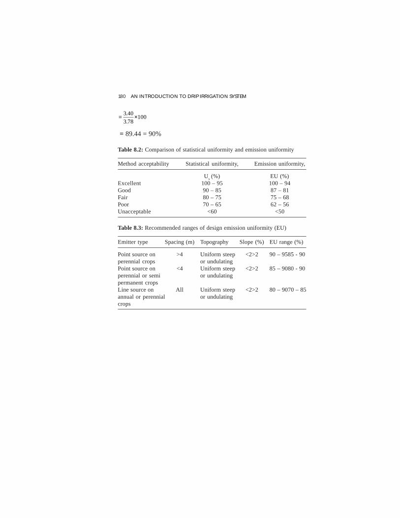
180 AN INTRODUCTION TO DRIP IRRIGATION SYSTEM
10078.3
40.3 ×=
= 89.44 = 90%
Table 8.2: Comparison of statistical uniformity and emission uniformity
Method acceptability Statistical uniformity, Emission uniformity,
Us (%) EU (%)Excellent 100 – 95 100 – 94Good 90 – 85 87 – 81Fair 80 – 75 75 – 68Poor 70 – 65 62 – 56Unacceptable <60 <50
Table 8.3: Recommended ranges of design emission uniformity (EU)
Emitter type Spacing (m) Topography Slope (%) EU range (%)
Point source on >4 Uniform steep <2>2 90 – 9585 - 90perennial crops or undulatingPoint source on <4 Uniform steep <2>2 85 – 9080 - 90perennial or semi or undulatingpermanent cropsLine source on All Uniform steep <2>2 80 – 9070 – 85annual or perennial or undulatingcrops

9Installation, Management and
Maintenance of Drip IrrigationSystems
Improper maintenance of the drip irrigation system can cause failureof the properly designed systems. The sensitivity of emitter to clogging,network of lateral pipes, filtration units and fertigation systems addthe complexities in the systems and need careful maintenance. Youcan maintain a system if it is appropriately installed. Proper installationcan ease your maintenance job. Let us first discuss about installationof drip irrigation system.
9.1. Installation
We assumed that a source of water already exists. Installation of thedrip irrigation system can be divided into three stages: (i) Fitting offilter units, (ii) Laying of mains and sub-mains, and (iii) Laying oflaterals with emitters.
9.1.1. Installation of Filter Unit
The following points should be considered for deciding the position offilter unit.
• There should be minimum use of fittings such as elbows andbends.
• The filter unit should be located on the delivery side of the pump.

182 AN INTRODUCTION TO DRIP IRRIGATION SYSTEM
• The filter size should be in accordance with the capacity of thesystem.
9.1.2. Installation of Mains and Sub-mains
Except for a fully portable system, both mains and sub mains areinstalled underground at a minimum depth of about 50–60cm suchthat they are unaffected by cultivation or by heavy agriculturalmachinery. Before laying PVC pipes in a trench, it may be paddedwith sand to avoid the expansion and contraction of compacted soils.Even for systems which have portable laterals that are removed at theend of each season, it is common practice to install permanentunderground sub-mains. Generally, sub-mains run across the directionof the rows.
9.1.3. Laying of Laterals
Generally, laterals are laid on the ground surface and placed alongcontours on sloping field. Laterals laid from the reels should be left onthe ground for 5-6 hours so that it can release the twisting formed inthe reel. The downstream end of the lateral can be closed by simplyfolding back the pipe and closing it with an end plug. This can beeasily slipped for flushing. The simplest connection for low-pressuresystem is for the lateral to be inserted directly into the sub-main. Cuttinga slightly undersized hole in the sub-main with either a wood auger bitor a metal twist drill is desirable. The hole is expanded with the taperedtool, and then the lateral is inserted quickly after withdrawing the taper.The lateral is cut at angle of about 450 at the end. When deciding thelateral length for installation, take into account that the lateral shrinks1 meter per 100 meters. Holes are made using punch on the lateral asper the required spacing. The on-line point source emitters should befixed such that outlets facing upward after laterals are spread on theground.
9.2. Testing of the System
Inspection at regular interval will ensure the proper functioning of thedrip systems. This can be done weekly, monthly or on seasonal basis,keeping in view the water quality and attributes of the system

INSTALLATION, MGNT. AND MAINTENANCE OF DRIP IRRIGATION SYSTEMS 183
components. Pump efficiency need to be tested at least once in 3 years.Higher pump efficiency, more than 80%, is desirable as it will alsosave the ever increasing energy cost. All the gate valves and flushvalves should be opened before testing. The filter should be backwashedtill clean water comes out through its flush valve. The flush valveshould be closed after flushing of sub-main. The working of air releasevalve is checked at the sub-main. The pressure at inlet and outlet ofthe filter should be obtained by regulating the bye-pass valve.Discharges from emitters are measured at normal operating pressureand their discharge variation and emission uniformities are determined.
9.3. Maintenance of Drip Irrigation System
The first step in maintaining a drip irrigation system is to take thesample of the water from the source which is going to be used. Thiswill help in determining the flushing requirement of the drip system.There are three types of clogging problems that need to be taken careof while preparing the maintenance program. These are physical,chemical and biological. Sand and silt may cause the physical hazardsto the system. Appropriate filtration technique is required to removeparticles above the maximum allowable particle size for the emittersbeing used. Chemical clogging hazards include the precipitation ofexcessive salt concentration. Irrigation water containing more than0.1 ppm sulphides can encourage the growth of sulphur bacteria withinthe irrigation system. Biological clogging hazards result from thegrowth of bacterial slimes and algae within drip lines and emitters.They combine with clay particles to block the emitters. Periodicpreventive maintenance is required for successful operation of a dripirrigation system. The general maintenance consists of following steps.
(a) The emitter functioning, wetting pattern and leakage of pipes,valves, and fittings should be checked regularly.
(b) The placement of emitters should be ascertained. If the placementis disturbed, put the emitters in proper location.
(c) Leakages through filter gaskets in the lids, flushing valves andfittings, etc. should be monitored regularly.

184 AN INTRODUCTION TO DRIP IRRIGATION SYSTEM
9.3.1 Flushing the Mainline, Sub-main and Laterals
During the installation process and before connecting the drip laterals,flush the main and sub-main lines. In case of failure or burst in themain or sub-main pipe, it is recommended to flush the dirt from linesby releasing the ends of the main and sub-main lines and flushingthem for at least 10 minutes. Filters usually do not prevent the entry ofsuspended particles and water soluble matter. Gradually over the time,a layer of sediment or organic matter settles in the main line and driplaterals. The end of the lateral line experiences the more accumulationof sediment and therefore it is recommended to flush the lines after 2-4 weeks of initial operation. Normally flushing 3-4 times per seasonwhen irrigating with good quality water (shallow/deep tube well), andat least once every fourth operation when irrigating with dirty water(ponds/canal) is suggested. During the crop growing period, daily checkup of screen/media filter performance and pressure and flow rate ofthe system should be carried out to meet the designed performance.Weekly observations on emitters clogging, cleaning of screens andstrainers can be made. Care must be taken on monthly basis regardingthe maintenance requirement of screen/media filter, comparison oflateral pressure to designed pressure and measuring of emitter dischargerate at selected locations.
9.3.2. Filter Cleaning
Filter is the core of a drip irrigation system and its failure will lead toclogging of the entire system. Keeping it serviceable and clean willprolong the life of the irrigation system. Pressure differential acrossthe filter is the correct indication of the timing of cleaning of the filter.Some of the steps are outlined here to maintain the filters.
1. Examine screens and seams to ensure that they are undamaged.
2. Ensure proper tightness between the screen, cover and body ofthe filter, in order to prevent lateral water leaks. If using a disctype filter, ensure the disc assembly is properly tightened.
3. Working with a partially clogged filter is detrimental to boththe filter and the quality of filtration. When the pressure

INSTALLATION, MGNT. AND MAINTENANCE OF DRIP IRRIGATION SYSTEMS 185
differential reaches approximately 5 meters, the system shouldbe flushed and cleaned.
4. Avoid entry of dirt into the pipe when the filter is opened forcleaning.
5. Flush the filter before irrigation operation starts. If the filter isvery dirty, clean more frequently. Automatic back-flushing maybe appropriate.
The cleaning procedures for various filters are given below.
9.3.2.1. Media Filter
The filter should be backwashed everyday for five minutes to removethe silt and other dirt accumulated during the previous day’s irrigation.Once in a week, while backwashing, the backwash water should beallowed to pass through the lid instead of the backwash valves. Thesand in the filter bed is stirred up to the filter candles without damagingthem. Whatever dirt is accumulated deep inside the sand bed will getfree and goes out with the water through the lid. For removal ofaggregates and algae, fill the container with chlorine and allowed tosoak for 24 hrs. After rinsing, pour off the water and leave the filter ina dry and ventilated place. Greasing and repair is done to avoid rustingas regular maintenance.
9.3.2.2. Screen Filter
The screens and sieves are needed to be examined to ensure that theyare undamaged. In order to prevent lateral water leakage, ensure propertightening of screens, cover and body of the filter. Before the start of adrip irrigation system, the flushing valve on the filter link is opened toflush out the dirt and silt. The filter element is taken out from the filterand it is cleaned in flowing water. The rubber seals are taken out fromboth the sides and precaution should be taken while replacing the rubberseals, otherwise they may get damaged.
9.3.3. Chemical Treatment
When normal flushing is not sufficient to clean the system and bring

186 AN INTRODUCTION TO DRIP IRRIGATION SYSTEM
uniform emission, chemical treatment is recommended. Clogging orplugging of emitters and orifices of bi-wall is due to precipitation andaccumulation of certain dissolved salts like carbonates, bi-carbonates,iron, calcium and manganese salts. The clogging is also due to thepresence of microorganisms and the related iron and sulphur slimesdue to algae and bacteria. The clogging of emitters is usually removedby chemical treatment. Chemical treatment commonly used in dripirrigation systems includes addition of chlorine and/or acid to the watersupply. The frequency of chemical treatment is decided on the degreeof clogging and quality of water. As a general rule, acid treatment isperformed once in ten days and chlorine treatment once in fifteen days.
9.3.3.1. Acid Treatment
Flushing with acid solution can dissolve the precipitation caused bydissolved salts. Hydrochloric acid (30%) is injected into the drip systemat the rate suggested in the water quality analysis report. All the sub-mains and laterals are flushed before the acid treatment and check thedischarge of the system before treatment. A solution equal to one tenth(1/10) of the maximum discharge of the injector pump is prepared andtreatment is performed till a pH of 4 is observed at the furthest lateral.After that irrigation is continued for 30 to 60 minutes.
9.3.3.2. Chlorine Treatment
Oxidation treatment is applied to decompose the organic matter andpreventing the building up of algae and bacteria. Chlorine is anoxidizing agent, which kills bacteria and other organic matter andprevents build up. The most common chlorine compounds are sodiumhypochlorite (liquid) and calcium hypochlorite (solid). There are threemain chlorine application methods:
1. Continuous Treatment
2. Superchlorination
3. Intermittent Treatment
1. Continuous Treatment: It is the simplest method of removingblockage problems in drip irrigation system. The water is treated

INSTALLATION, MGNT. AND MAINTENANCE OF DRIP IRRIGATION SYSTEMS 187
continuously to keep the system clean from organic material. Therequired concentration varies according to water quality. Usuallythe injection rate is adjusted such that 1 ppm of chlorine isdetectable at the end of the furthest lateral from the pump. Thecommon concentration to begin with is usually 5-10 ppm (mg/l).
2. Superchlorination: When the irrigation system has operatedfor some time and there is an accumulation of organic matterinside the pipeline, superchlorination is needed to dissolve theorganic slime. Chlorine is normally injected at a concentrationof 500 ppm. The system is shut down and left for 24 hrs. Thesystem is then flushed step-by-step, first main line, then sub-main, and finally through the end of the laterals.
3. Intermittent Treatment: Although the filter system operatesproperly, microorganisms such as algae, fungi and bacteria maypass through it into the irrigation system. To prevent a build-up ofthis organic matter in the laterals, periodic sterilization bychlorination is needed. During the last hour of irrigation, chlorineconcentration of 10-20 ppm is applied for 30 minutes in the irrigationwater. The chlorine is left in the pipe until the next irrigation.
The rate of injection of liquid chlorine or acid depends on the systemflow rate and can be determined by
'cs
uQK
cq = ….................................................................... (9.1)
where,
qc = rate of injection of the chemical into the system, lph
K = conversion constant, 3.6 × 10⁻³ for metric units
u = desired dosage in irrigation water, ppm
Qs = irrigation system discharge capacity, lps
C = concentration of the desired component in liquid chemicalconcentrate, kg/l
Chlorination should be used regularly to kill algae and loosen bonded

188 AN INTRODUCTION TO DRIP IRRIGATION SYSTEM
organic matter within the system for flushing out. It has no effect onscale (lime or calcium carbonate) deposits in the system. Liquid sodiumhydrochloride is the recommended chlorine source. It is injected intothe system during regular operation usually using the fertigationequipment. Rates of 5 to 20 ppm chlorine may be required, dependingon the severity of the problem. It is essential to measure the activechlorine in the irrigation water at the start and end of the system duringchlorination to ensure that the required concentrations are reached.Chlorine is more effective in acid waters. High pH or alkaline watersshould be acidified to a pH of 6.5 for effective chlorine treatment. TheEq. 9.1 may be given in a different form with easier units as follows.
100
1
××
=C
QCq …........................................................................ (9.2)
where
q = discharge of injected chlorine solution, lph
Co
= percentage of active chlorine in injected solution
C1 = desirable concentration of active chlorine in irrigation water, mg/l
Q = discharge of the treated system, m3/h
Example 9.1. In drip irrigated vegetable plot, the system flow rate is125m3/h. Active chlorine percentages in the solution was 10% and thedesired concentration is 15mg/l. Estimate the discharge of injectedchlorine solution.
Solution. We can apply Eq. 9.2 and find the result. Applying theequation, we get
1010
12515
××=q
= 18.75 lph

10Salt Movement Under Drip
Irrigation Systems
Irrigation requires relatively large quantities of water. Appropriateselection of crops, irrigation methods and management practices canenable us to utilize wide range of irrigation water quality. Non-conventional water resources such as saline drainage water, brackishgroundwater and treated wastewater are alternatives to fresh waterresources. However, careful management is required to safeguard theenvironment and promotes sustainable agricultural production withoutdegrading our land and water resources. In conventional surfaceirrigation systems, the whole field is flooded with irrigation water andusually the water flow through the soil is one dimensional. Excesswater drains out of the root zone and helps in leaching of salts out ofthe root zone. In case of drip irrigation systems, when emitters areplaced above the soil surface, two dimensional water flows occurswithin the soil where only portion of the soil surface is wetted. Similarly,three dimensional water and salt movement occurs within the root zonewhere the emitters are placed beneath the soil surface as in case ofsub-surface drip irrigation. Under these conditions, excess water doesnot flow into deep drainage and also does not allow leaching the saltbelow the root zone. For example, some of the water moving from aburied drip irrigation emitter will move laterally or up towards the soilsurface. When water arrives at the soil surface, it is evaporated, andthe residual salt accumulates on the surface which may be leachedback into the root zone by subsequent rainfall (Fig.10.1). It has been

190 AN INTRODUCTION TO DRIP IRRIGATION SYSTEM
Fig.10.1: Salt rings formed on soil surface around drip irrigation of grapes dueto evaporation of irrigation water (Courtesy- G. Schrale).

SALT MOVEMENT UNDER DRIP IRRIGATION SYSTEMs 191
observed that in arid and semi-arid regions, the salt accumulation inthe root is always a concern for farmers irrigating crops with dripirrigation systems.
Surface evaporation and net flux of water across the soil surface underdrip irrigation is spatially variable. At and near the dripper, the netwater flux will likely be downwards, but further away evaporativefluxes will exceed infiltration, especially during dry periods, leadingto an upward flux of water. The use of surface mulches which reduceevaporative fluxes can have a large impact of the direction andmagnitude of vertical water and salt flux. It has been reported thatirrigation during the day time, produces different soil-waterdistributions to irrigations conducted at night time due to differencesin upward flux. Thus at the end of a dry summer, during which a crophas been drip irrigated, salt patterns are likely to be highly variable.Winter rain could leach salt, but may be insufficient to leach salt fromareas of high concentration. In some cases, rainfall may mobilize saltpreviously accumulated on the soil surface back into the root zonecreating an adverse impact on root zone osmotic potentials (Raineet al., 2005). Cote et al. (2003) simulated the flow of a pulse of solutesfrom drip irrigation and showed that solute applied at the end of theirrigation ends up deeper in the soil compared to when it was appliedat the start of the irrigation, owing to an increase in the ratio ofdownward to lateral water flux over time. This is completely differentto what would happen for one dimensional flow. Such studies suggestthat much more research is required to understand solute transport indrip systems especially over an irrigation cycle and the interactionwith rainfall events. Plant roots also play a major role in soil-waterand solute dynamics by modifying the water and solute uptake patternsin the rooting zone. Also the implementation of drip irrigation systemsraises the vital issues in relation to soil-water and salt management.The adoption of drip irrigation technologies and practices can result inroot zone salinisation problems. The leaching calculated using onedimensional equation may not adequately describe leaching under somefield conditions.
Normally the reclamation of salt affected soil is done by leaching the

192 AN INTRODUCTION TO DRIP IRRIGATION SYSTEM
salts beyond root zone. Idea is to pond the water over the entire fieldand allows it to leach. To do this, sprinklers or furrows can be usedvery well. However, with drip irrigation, salt accumulation takes placemainly along the tree rows as visible in Fig.10.1. Therefore, leachingwater need not to be applied to the whole field. In this case, water isapplied to 1/3 of the field area which only one third of the amount ofleaching water is needed as compared to the conventional leachingtechniques. This approach significantly saves the water. Four to sixlateral lines are placed at a spacing of 40-50cm along one row of plantsmainly fruits crop to apply leaching water to the salt accumulated soilarea. Efforts must be made to achieve high leaching efficiency i.e.removal of the maximum salt per unit of leaching water. Leachingwater is normally applied for 24 hours and the stopped for 3-4 daysand started for another 24 hours. Soil samples may be collected after4-5 days of application of last leaching water to check the salinitylevel in crop root zone.
10.1. Salinity Measurement
Salts in saline soils originate from the natural weathering of mineralsor from fossil salt deposits left from ancient sea beds. On arid or semi-arid regions, salts accumulate when the irrigation water or groundwaterseepage evaporates. Examples of common salt compounds are SodiumChloride (NaCl), Sodium Sulfate (Na
2SO
4), Magnesium Sulfate
(MgSO4), Calcium Sulfate (CaSO
4), and Calcium Carbonate (CaCO
3).
An electrical current is passed through a soil solution extract to measuresalinity of the soil The ability of the soil solution extract to carry acurrent is called electrical conductivity (EC). EC is measured indeciSiemens per meter (dS/m), which is the numerical equivalent tothe millimhos per centimeter. The lower the salt content of the soil, thelower the dS/m rating and the less the effect on plant growth. Yields ofmost crops are not significantly affected where salt levels are 0 to 2dS/m. Generally, a level of 2 to 4 dS/m affects some crops. EC isrelated with total cations and osmotic pressure of soil water extract,the following expressions can be used to evaluate the saltconcentrations.

SALT MOVEMENT UNDER DRIP IRRIGATION SYSTEMs 193
Salt concentration (ppm) = 640 x EC (millimhos/cm) ............. (10.1)
Total cation concentration (meq/l) = 10 x EC (millimhos/cm) ..(10.2)
Osmotic pressure (atm.) = 0.36 x EC (millimhos/cm) …......... (10.3)
We know that 1 ppm is equal to 1 mg/l and if ppm is divided by theequivalent weight, we get meq/l.
Example10.1. It is given that electrical conductivity of the soil waterextract is 8 millimhos/cm. Convert it into ppm, micromhos, and mhos/cm.
Solution. Electrical conductivity (EC) of the soil water extract = 8millimhos/cm
= 8/100 = 0.08 mhos/cm
=8x1000=8000 micromhos/cm
As we know that
Salt concentration (ppm) = 640 x EC (millimhos/cm)
= 640 x 8
= 5120 ppm
10.2. Leaching Requirements
Ragab (2002) reported that soil salinity does not reduce crop yieldsignificantly until a threshold level is exceeded. To avoid yield losswhen salt concentrations exceed their tolerance limits, excess saltsmust be leached below the root zone. Thus, when the net depth ofapplied water is calculated for scheduling, an additional depth of waterbased on the salinity level should be added for leaching. The leachingrequirement (LR) is usually calculated as:
d
i
i
d
C
C
D
DLR == ….................................................................. (10.4)
where,
Dd = depth of water passing below the root zone as drainage water

194 AN INTRODUCTION TO DRIP IRRIGATION SYSTEM
Di = depth of applied irrigation and rainfall water
Cd = salt concentration of the drainage water above which yield
reduction occurs
Ci = salt concentration of the irrigation water.
The initial equation developed by (Reeve et al., 1967) is given as
NN
N
d
i
D
W
LD
L
C
C
EC
ECLR
+=== …...................................... (10.5)
where
ECW = electrical conductivity of irrigation water
ECD = electrical conductivity for water draining under the root zone;
LN
= net annual leaching requirement, mm
DN = net annual depth of irrigation to meet consumptive use of water, mm
Bernstein (1973) reported the following equations to determine theleaching requirement.
( )WE
W
ECEC
ECLR
−=
5…............................................................... (10.6)
but to measure leaching requirement under drip irrigated crops, thefollowing equation was suggested.
E
W
EC
ECLR
max2×= …................................................................. (10.7)
where, ECE is electrical conductivity corresponding to 100% yield loss.
Example10.2. Under a drip irrigated plot, the EC of the saturated soilpaste was recorded as 9 millimhos/cm and EC corresponding to 100%yield loss was 13 millimhos/cm. Find out the leaching requirement.
Solution. We will apply Eq.10.7
E
W
EC
ECLR
max2×=

SALT MOVEMENT UNDER DRIP IRRIGATION SYSTEMs 195
100132
9 ××
=
= 34.62 = 35%
10.3. Salt Tolerance of the Crop and Yield
Under drip irrigation system, frequent application of water is providedwhich keeps the salt concentration in the soil to a minimum. Frequentirrigation usually keeps the salt concentration in the soil water almostequal to the salt concentration in irrigation water. But if irrigationinterval is increased, the salt accumulation can take place as the rootzone soil dries. It has been observed that with poor quality irrigationwater, crop yield under drip irrigation systems is usually higher thanthat of other methods of irrigation with the same quality of irrigationwater. This is mainly attributed to the fact that salts remain diluted bythe continuous supply of irrigation water. Information of electricalconductivity of irrigation water and saturated soil extract are essentialfor salinity management. To determine the relative yield, maximumelectrical conductivity of saturated soil extract is necessary. This issomething at which yield of the crop will be zero. The maximumelectrical conductivity of saturated soil extract (EC
E)
for several crops is give in Table 10.1 (Keller and Blisener, 1990). Ifthe electrical conductivity of irrigation water (EC
W) is lying between
the minimum ECE and (EC
E max + EC
E min)/2, then relative crop yield
(YR) can be obtained from the following expression.
EE
WER ECEC
ECECY
minmax
max
−−
= …....................................................... (10.8)
where,
min ECE = electrical conductivity of saturated soil extract that will not
decrease crop yield, dS/m
max ECE
= electrical conductivity of saturated soil extract that willdecrease crop yield to zero, dS/m
Example 10.3. A well developed lemon orchard under drip irrigation


SALT MOVEMENT UNDER DRIP IRRIGATION SYSTEMs 197
This means that if full potential of yield is 100 t, then with this salinitylevel of irrigation water, 76 t of produce will be obtained.
10.4. Saltmed Model
There are many single-process oriented model such as (i) models forinfiltration (ii) models for root water uptake (iii) models for leachingor water and solute transport or (iv) models for specific applications,i.e. certain irrigation system, soils, region or a crop. The need forcomprehensive generic models that account for different crops, waterand field management practices was addressed by developing theSALTMED model (Ragab, 2002). The model employs well establishedwater and solute transport, evapotranspiration and crop water uptakeequations and successfully illustrated the effect of the irrigation system,the soil type and irrigation salinity level on soil moisture and salinitydistribution, leaching requirements, and crop yield in all cases. Themodel successfully predicted the impact of salinity on yield, wateruptake, soil moisture and salinity distribution. The model providesacademics with a research tool and field managers with a powerfultool to manage their water, crop and soil in an effective way in order tosave water and protect the environment.
Table 10.2: Minimum and maximum values of electrical conductivity ofsaturated soil extract (EC
E)
Crops ECE
Crops ECE
Min Max Min Max
Field cropsCotton 7.7 27 Corn 1.7 10Sugarbeet 7.0 24 Flax 1.7 10Sorghum 6.8 13 Broadbeans 1.5 12Soybean 5.0 10 Cowpeas 1.3 8.5Sugarcane 1.7 19 Beans 1.0 6.5Fruits and nut cropsDate palm 4.0 32 Apricot 1.6 6Fig. olive 2.7 14 Grape 1.5 12Pomegranate 2.7 14 Almond 1.5 7Grapefruit 1.8 8 Plum 1.5 7
Contd.

198 AN INTRODUCTION TO DRIP IRRIGATION SYSTEM
Orange 1.7 8 Blackberry 1.5 6Lemon 1.7 8 Boysenberry 1.5 6Apple, pear 1.7 8 Avocado 1.3 6Walnut 1.7 8 Raspberry 1.0 5.5Peach 1.7 6.5 Strawberry 1.0 4.0Vegetable cropsBeets 4.0 15 Pepper 1.5 8.5Broccoli 2.8 13.5 Lettuce 1.3 8.0Tomato 2.5 12.5 Radish 1.2 9.0Cucumber 2.5 10 Onion 1.2 7.5Spinach 2.0 15 Carrot 1.0 8.0Cabbage 1.8 12 Beans 1.0 6.5Potato 1.7 10 Turnip 0.9 12.0
10.4.1. Equations of the Model
The SALTMED model addresses the important processes such asevapotranspiration, plant water uptake, water and solute transport underdifferent irrigation systems including drip irrigation, drainage and theinterrelationship of crop yield and water use. The evapotranspirationhas been estimated by using the Modified Penman–Monteith equation.In case the weather data such as temperature, radiation and wind speed,etc. are not available, the model can use pan evaporation data tocalculate the evapotranspiration. The effective rainfall is defined asthe part of the rainfall that is available for infiltration through the soilsurface. The model estimates it in three ways: (i) as a percentage oftotal rainfall (ii) calculate according to the FAO-56 (1998) procedure,and (iii) taken to be equal to total rainfall. The water uptake rate formulasuggested by Cardon and Letey (1992a), which determines the wateruptake S per day as given below:
λ
ππ
.3.
150
++=
ha
SS MAX
….......................................................... (10.9)
Crops ECE
Crops ECE
Min Max Min Max

()Z
HhKq
δδ−=

200 AN INTRODUCTION TO DRIP IRRIGATION SYSTEM
( ) ( )wS
z
zK
zt−
∂+∂
∂∂−=
∂∂ ψθθ
….................................... (10.16)
where, θ is volume wetness; t is the time; z is the depth; K(θ) is thehydraulic conductivity; ψ is the matrix suction head; and S
W is the
extraction by plant roots. The movement of solute in the soil systemdepends greatly on the path of water movement. For detail information,please refer to Ragab (2002). The leaching requirement is calculatedin the SALTMED model as a ratio of the salt concentration of theirrigation water to that of the drainage water or the mean salinity levelof the root zone as given in Eq. 10.4.
The input data requirement of the model are plant characteristics foreach growth stage, soil characteristics, weather data, and watermanagement data include the date and amount of irrigation waterapplied and the salinity level of each applied irrigation (Fig. 10.2). Agood number of data are available in the databases of the model suchas crop database, soils database which contains the hydrauliccharacteristics and solute transport parameters of more than 40 differenttypes of soils and irrigation system database. The model is able toanalysis the effect of the different irrigation systems, soil type, theirrigation salinity level on soil moisture and salinity distribution,leaching requirements, and crop yield. Figure 10.3 indicate that nearthe emitter, the soil salinity is less.

SALT MOVEMENT UNDER DRIP IRRIGATION SYSTEMs 201
Fig. 10.2: Input parameter of SALTMOD model (Ragab, 2002)
Fig.10.3: Soil salinity profile under emitter (Ragab, 2002)


11Automation of Drip Irrigation
Systems
Automation of drip irrigation system refers to operation of the systemwith no or minimum interventions of operators. Automation is mostsuitable to drip irrigation systems because it supplies controlled andpre-determined amount of irrigation water to irrigate large area fromthe same source of water. It is always inconvenient to precisely irrigatethe farm field without automation. Let us take an example, you maynot get labor to operate drip systems frequently and that too for shortdurations of time, which in many cases is required to maximize yieldsand avoid wasting of water and other valuable inputs. The problemworsens if it is required to turn valves on for a few seconds after every30-40 minutes. It has been realized that controllers and valves arecost effective and reliable, leaving labor to perform other and moreimportant tasks to grow a better crop. Nowadays relatively inexpensivecontrollers and valves are available in the market which can be installedin any application with little effort. Controllers are available forapplications with or without power, and for situations where simplicityand low cost are the key factors. Solenoid activated valves are availablein a multitude of sizes and configurations, and are equally simple andcost effective. Besides above, automation of irrigation systems providesthe following advantages.
• It saves our precious water.
• It starts and stops irrigating at the pre-determined or programmedtime.

204 AN INTRODUCTION TO DRIP IRRIGATION SYSTEM
• It can take into account the effective rainfall for schedulingirrigation.
• No need to visit farm at odd times.
• Adequate quantity of water and nutrients supply result in qualityproduce and high yield.
• No leaching of minerals and nitrogen vital for plants healthygrowth.
• Avoid the ill effects of over irrigation which causes developmentof salinity.
• System can be operated at night, thus the day time can be utilizedfor other agricultural activities
11.1 Types of Automation
Automation systems are classified on the basis of type and scope ofcontrol or even time can be the basis of operation. The basic objectiveis to prepare a schedule based on crop water requirements. First let usdiscuss the classification of automation on the basis of type of control.On the basis of type of control, the automated irrigation systems canbe classified in to two categories i.e. sequential and non- sequentialtype. In sequential systems, the field is divided in to different smallerunits, which is irrigated one at a time in a well laid out sequence,whereas in the non-sequential systems, the smaller units are irrigatedrandomly based on the crop water needs. Sequential system can beclassified as (i) Hydraulically operated, (ii) Electrically operated, and(iii) Combination of above two methods.
11.1.1. Hydraulically Operated Sequential System
The sequential system is particularly suited for irrigation at lowdischarges through small-diameter tubing. The water metering deviceand a hydraulic valve are located at each connection to the main line(Fig.11.1). The metering valves are pre-set for the required amount ofwater to be applied to the field or sub-plots in the beginning of theirrigation cycle. The amount of water is determined according to crop

AUTOMATION OF DRIP IRRIGATION SYSTEMS 205
water requirement. Water under pressure passes through the firstmetering valve to the hydraulic valve on the main line and stops theflow of water. The metering valve closes after the pre-determinedquantity of water has passed through the first head. The pressure at thehead of the hydraulic valve is released, and the water pressure of themain line opens the next valve. Thus the irrigation is completed in allthe group of drip laterals. Such types of systems are suitable forgreenhouses, gardens, and nurseries.
Fig. 11.1: Sequential hydraulic operated automated irrigation system.

206 AN INTRODUCTION TO DRIP IRRIGATION SYSTEM
11.1.2. Volume Based Sequential Hydraulically AutomatedIrrigation System
This type of system is suitable for irrigating orchards and field cropsand any pipe diameter ranging from 50 to 254 mm and handle relativelylarge flow of water. The system can operate on a main line andautomatically open the valves on the laterals. The system consists ofhydraulic automatic metering valves, with or without an arrangementfor cumulative readings of the quantity of water discharged (Fig. 11.2).Each metering valve can operate as an independent unit or can also beused to activate a number of supplementary hydraulic valves. Thedischarge of such units depends on the maximum quantity of water, whichmay pass through the line without any excessive friction losses. At thestart of irrigation cycle all the metering valves are pre-set to the requiredquantities of water. The water flow reaches the first metering valve after
Fig. 11.2: Volume based sequential hydraulic system.

AUTOMATION OF DRIP IRRIGATION SYSTEMS 207
opening of the main valve. The water pressure is transmitted from thefirst metering valve through the hydraulic tubing and keeps the secondmetering valve closed. When the desired quantity of water has beendelivered to the first sub-plot, the first metering valve closes.The pressureon the second metering valve is released and the water pressure on themain supply line opens the next valve. This cycle is repeated until thelast lateral is opened and the entire irrigation cycle is completed.
11.1.3. Time Based Electrically Operated Sequential System
Sequential electrically operated systems operate in sequence to controlirrigation. The remotely placed solenoid valves with electric currentthrough cables control water application. In this system, the waterquantity delivered to the different plots is regulated by timer clock.The time clock is programmed to start and stop at desired time by theuser. These types of controllers are usually designed with calendarprograms so that the watering cycle can be automatically started onthe desired day of the week. This system was developed mainly for theirrigation of domestic gardens and sprinkler irrigation but in principleit can be used for any kind of permanent irrigation. Regular solenoidvalves are used for handling the low-pressure discharge. Sequentialhydraulically–electrically operated system uses solenoid valves toactivate hydraulic valves and the over all operation is hydraulic-electric.Rest of its operation is similar to sequential electrically operated system.Such types of systems are used for large diameter pipes.
11.1.4. Non-sequential Systems
Electrically controlled non-sequential systems are automatic to a greaterextent as compared to that of sequential systems. These systems controlelectric or hydraulic valves, which operate independently in terms ofthe quantity of water to be applied or frequency of irrigation. Water ineach unit is supplied in different quantity and valve opens at a differenttime in response to a pre-determined program or to soil water content.The control panel contains electrical circuits to operate the pump ormain valve, to add fertilizer according to a pre-set schedule, and tomeasure soil moisture so that irrigation can be supplied to meet cropneed. Such systems are usually remote-controlled, and are designed

208 AN INTRODUCTION TO DRIP IRRIGATION SYSTEM
for feedback of the data received from the field so that automaticregulation can be taken up and adjustments for changes in the pressureand discharge rate of the supply line can be accommodated. Non-sequential systems are further classified into three categories i.e. (i)Feedback control, (ii) Inferential control.
11.1.4.1. Feedback Control System
The main components of the feedback control system are soil moisturesensors, electronic control unit such as comparators, microprocessor,computer, and solenoid valves. A farm is divided in to different sub-plots.Each sub-plot has one soil moisture sensor. The sensors are connectedthrough proper interfacing circuit to the central control unit. The centralcontrol unit is a microprocessor or a computer which can be instructed totake up a program to make irrigation scheduling decisions or comparatorcircuit (Fig. 11.3). Based on the soil moisture status of a sub-plot, controllerdecides when to start and stop the irrigation. The electronic controlleractuates and de-actuates solenoid valves to start and stop the irrigationthrough proper interfacing circuit and relay switches.
Fig. 11.3: Components of computer controlled irrigation system and their layout

AUTOMATION OF DRIP IRRIGATION SYSTEMS 209
11.1.4.2. Inferential Control System
This system is basically based on available evapotranspiration modelsto determine evapotranspiration of crop using weather parameters. Theestimated evapotranspiration is used to schedule irrigation. The mainparts of inferential control system are sensors for measuring variousweather, evapotranspiration model, and solenoid valves. The solenoidvalves are operated using interfacing circuit and relay switches to puton or to put off the irrigation system.
11.2. Components of Automated Irrigation System
An automated irrigation comprises of components such as sensors,communication lines, controllers and actuators. Sometime fertigationunits, filters and back flush device for filters have also automatedoperation with drip irrigation system. The description of different typesof soil moisture sensors, communication cables, controllers andactuators are briefly presented in the following section.
11.2.1. Irrigation Controllers
This is one of the most important components of an automated irrigationsystem. It turns the irrigation system on and off at the pre determinedtimes. In other words, the controller controls the irrigation system andthe operator controls the controller. The right controller may cause theconsiderable water savings and lower energy bills. There may be oneseparate valve that controls the flow of water to a specific crop. Thecontroller can be programmed to determine when, how frequent, andhow long each valve is open. The controller should have programmingflexibility so that water can be applied more efficiently.
11.2.2. Soil Moisture Sensors
Soil moisture sensors measure the water content in the soil. Soilmoisture sensors commonly used for automation purpose aretensiometer and resistance block type.
Tensiometer
The tensiometer is a device, which provides direct measure of tenacity

210 AN INTRODUCTION TO DRIP IRRIGATION SYSTEM
with which water is held by the soil. Tensiometers are commerciallyavailable in numerous configurations. The main disadvantage of thetensiometer is that it functions only from 0.0 to about -0.8 bar, whichrepresents a small part of the entire range of available water. The lowermoisture limit for the good crop growth is beyond the tensiometer range.Any change in soil water causes corresponding change in soil moisturetension. In automated irrigation systems, the tensiometer is modifiedto read change in soil moisture tension in terms of change in voltage orresistance.
Resistance Blocks
In this type of sensor, the electrical resistance between the twoelectrodes varies with moisture of resistance block, which is inequilibrium with the soil moisture in the crop root zone. The presenceof salt or salinity in irrigation water or soil affects the observations.The gypsum block and granular matrix type sensors are commonlyused for soil moisture sensing.
Gypsum Block
One of the most common methods of estimating matric potential iswith gypsum or porous blocks. The device consists of a porous blockcontaining two electrodes connected to a wire lead. The porous blockis made of gypsum. When the device is buried in the soil, water willmove in or out of the block until the matric potential of the block andthe soil are the same. The electrical conductivity of the block is thenobserved. A calibration curve is made to relate electrical conductivityto the matric potential for any particular soil. The disadvantage of theporous block system is that each block has different characteristicsand must be individually calibrated. Gypsum blocks are easy to useand economical but the inherent disadvantage with this sensor is thatgypsum dissolves with water, calibration curve changes with the timein the same location.
Granular Matrix
These sensors reduce the problems inherent in gypsum blocks by use
AUTOMATION OF DRIP IRRIGATION SYSTEMS 211
of a granular matrix which is supported in a metal or plastic screen.The electrodes inside the sensors are embedded in the granular fillmaterial above the gypsum wafer. The gypsum wafer slowly neutralizesthe salinity of the soil solution hence electrical resistance between theelectrodes is unaffected. Particle size of the granular fill material andits compression determines the pore size distribution in sensor. Suchsensors require little maintenance during the growing season and suitedfor sensing soil water potential and automatic control of irrigationsystems. They have advantages of low unit cost and simple installationprocedures similar to those used for tensiometers.
Sensors for Climatological Parameters
Sensors for measuring various climatological parameters such as solarradiation, maximum and minimum temperature, wind speed, relativehumidity, pan evaporation etc. are interfaced to the computer to estimateevapotranspiration of crop and irrigation is commissioned based onevapotranspiration demand. Sensor to measure evaporation from a panis interfaced with irrigation controller to actuate and deactuates theirrigation system.

212 AN INTRODUCTION TO DRIP IRRIGATION SYSTEM
ReferencesAh Koon, P.D., P.J. Gregory, and J.P. Bell. 1990. Influence of drip irrigation
emission rate on distribution and drainage of water beneath a sugarcane and a fallow plot. Agric. Water Manage. 17:267–282
American Society of Agricultural Engineers. 1985. ASAE Engineering Practice,ASAE EP405.
American Society of Civil Engineers, Committee on Irrigation WaterRequirements of the Irrigation and Drainage Division of the ASCE.1990. Evapotranspiration and Irrigation Water Requirements: a Manual.332 p.
Amin, M.S.M. 1990. Hydraulic analysis of trickle lateral. Ph.D. thesis,Southampton University.
Anonymous. 1984. Code for Design and Installation of Trickle Irrigation System,Indian Standard Code IS:10799 (Part 1), 1-15.
Anwar, A.A. 1999. Factor G for pipelines with equally spaced multiple outletsand outflow. J. Irrig. and Drain. Engrg., ASCE, 125(1):34-38.
Assouline, S., Cohen, S. Meerbach, D. Harodi, T. and Rosner, M. 2002.Microdrip irrigation of field crops: Effect on yield, water uptake, anddrainage in sweet corn. Soil Sci. Soc. Am. J. 66:228-235.
Badr, A.E., Ebabi, F.G., ELtomy, E.O. 2006. Fertigation methods effects onwater and fertilizer uniformity in drip irrigation. Misr J. Ag. Eng.,23(1):122-136.
Bernstein, L. and L.E. Francois, 1973. Leaching requirement studies: Sensitivityof alfalfa to salinity of irrigation and drainage water. Soil Sci.Soc. Amer.Proc., 37:931-943.
Blaney, H.F., Criddle, W.D. 1950. Determining Water Requirements in IrrigatedAreas from Climatological Irrigation Data. Technical Paper No. 96, USDepartment of Agriculture, Soil Conservation Service, Washington, D.C.,48 pp.
Bralts, V.F., Segerlind, L.J. 1985. Finite elements analysis of drip irrigationsubmains units. ASAE, 28(3):809-814.
Bralts, V.F., Kelly, S.F., Shayya, W.H., Segerlind, L.J. 1993. Finite elementsanalysis of micro-irrigation hydraulics using virtual emitter systems.ASAE, 36(3):717-725.
Bowen, I.S. 1926. The ratio of heat losses by conduction and by evaporationfrom any water surface. Phys. Rev. 27:779-787.
Cardon, E.G., Letey, J., 1992b. Soil-based irrigation and salinity managementmodels: II, water and solute movement calculations. Soil Sci. Soc. Am.J. 56:1887-1892.
Christiansen, J.E. 1942. Hydraulics of sprinkling systems for irrigation. ASCE,107:221-239.
Clapp, R.B. and G.M. Hornberger, 1978. Empirical equations for soil hydraulicproperties.- Water Resources Research, 14:601-604.
Coelho, E.F., and D. Or. 1996. A parametric model for two-dimen-sional water

AUTOMATION OF DRIP IRRIGATION SYSTEMS 213
uptake by corn roots under drip irrigation. Soil Sci. Soc. Am. J. 60:1039-1049
Coelho, E.F., and D. Or. 1999. Root distribution and water uptake patterns of cornunder surface and subsurface drip irrigation. Plant Soil 206, pp.123-136.
Cote, C.M., Bristow, K.L., Charlesworth, P.B., Cook, F.J. and Thorburn, P.J.2003. Analysis of soil wetting and solute transport in subsurface trickleirrigation. Irr. Sci., 22:143-156.
Dalton, J. 1802. ‘Experimental essays on the constitution of mixed gases: onthe force of steam or vapour from water or other liquids in differenttemperatures, both in a Torricelli vacuum and in air; on evaporation;and on expansion of gases by heat. Manchester Lit. Phil. Soc. Mem.Proc., 5:536-602.
Drnevich, V.P., Ashmawy, A.K., Yu, X., Sallam, A.M. 2005. Time domainreflectometry for water content and density of soils: study of soil-dependent calibration constants. Can. Geotech. J. 42:1053-1065.
Evett, S.R., Howell, T.A., Tolk, J.A. 2005. Time domain reflec-tometrylaboratory calibration in travel time, bulk electrical conduc-tivity, andeffective frequency. Vadose Zone J. 4:1020-1029.
Hahn, R.H., Rosentreter, E.E. 1995. American Society of Agricultural Engineers(ASAE) Standards. St. Joseph, Michigan.
Hargraves, G.H., Samani, Z.A. 1982. Estimating PET, Tech Note, J. Irrig. DrainEng., 108(3):225-230.
Hargraves, G.H., Samani, Z.A. 1985. Reference Crop Evapotranspiration fromTemperature, Appl. Eng. Agric., 1(2):96-99.
Hartz, T.K., Smith, R.F. LeStrange, M. and Schulbach, K.F. 1993. On-farmmonitoring of soil and crop nitrogen status by nitrate-selective electrode.Commun. Soil Sci. Plant Anal., 24:2607-2615.
Hartz, T.K. and Hochmuth, G.J. 1996. Fertility management of drip-irrigatedvegetables. Hort Technology, pp.168-172.
Hathoot, H.M., Al-Amoud, A.I., Mohammad, F.S. 1993. Analysis and designof trickleirrigation laterals. American Society of Civil Engineers. Journalof Irrigation and Drainage Division, 119(5):756-767.
Hawkins, A.J. 1985. Electrical Sensor for Sensing Moisture in Soil. US Patent5179347, Date issued 12th January.
Helmi, M.H., Ahmed, I.A.A., Fawzi, S.M. 1993. Analysis and design of trickleirrigation laterals. ASCE, 119(5):756-767.
Hochmuth, G.J. 1994. Sufficiency ranges for nitrate-nitrogen and potassiumfor vegetable petiole sap quick tests. Hort Technology, 4:218-222.
Howell, T.A., Hiler, E.A. 1974. Trickle irrigation lateral design. ASAE, 17(5):902-908.
Howell, T.A., Barinas, F.A. 1980. Pressure losses across trickle irrigation fittingsand emitters. Trans ASAE, 23(4):928-933.
Howell, T.A., Holer, E.A. 1974. Designing trickle irrigation laterals foruniformity. Journal of Irrigation and Drainage Div. ASCE, 100(IR4):443-445.

214 AN INTRODUCTION TO DRIP IRRIGATION SYSTEM
Howell, T.A., Stevenson, D.S. Aljibury, F.K. Gitlin, H.M. Wu, J.P. Warrick,A.W. and PAC. Raats. 1982. Design and operation of trickle (drip)system. In Design and Operation of Farm Irrigation System, ed. M.E.Jensen, Chpt. 16.ASAE Monograph No.3.
James, G.L. 1988. Principles of Farm Irrigation System Design. John Wiley &Sons, Inc. USA.
Jensen, M.C., and Fratini, A.M. 1957. Adjusted ‘F’ factors for sprinkler lateraldesign. Agric. Engrg., 38(4):247.
Jensen, M.E. 1980. Design and Operation of Farm Irrigation Systems. ASAEMonograph 3, American Society of Agricultural Engineers. St. Joseph,Michigan.
Jeppson, R.W. 1977. Analysis of Flow in Pipe Networks. Ann Arbor Science,Michigan.
Kang, Y., Nishiyama, S. 1994. Finite element method analysis of micro-irrigationsystem pressure distribution. Trans., Japanese soc. of irrig., drain., andreclamation eng., Tokyo, Japan, 169:19-26
Kang, Y., Nishiyama, S. 1996a. Analysis and design of microirrigation laterals.American Society of Civil Engineers. Journal of Irrigation and DrainageDivision. 122(2):75-81.
Kang, Y. Nishiyama, S. 1996b. Design of microirrigation submain units.American Society of Civil Engineers. Journal of Irrigation and DrainageDivision, 122(2):83-89.
Karmeli, D., Keller, J. 1975. Trickle Irrigation Design. Glendora, California:Rain Bird Sprinkler Manufacturing Corp.
Keller, J., Karmeli, D. 1974. Trickle irrigation design parameters. ASAE, 17(4):678-684.
Keller, J., Ron, D. Bliesner (Editors). 1990. Sprinkler and Trickle Irrigation.Van Nostrand Reinhold, New York.
Koenig, E. 1997. Methods of micro-irrigation with very small discharges andparticularly low application rates. (In Hebrew.) Water Irrig. 365:32-38.
Lakhdar, Z., Dalila, S. 2006. Analysis and design of a microirrigation lateral.Journal Central European Agriculture. 7(1):57-62.
Martin, E.C. 2009. Methods of Measuring for Irrigation Scheduling - WHEN.AZ1220, Arizona Water Series No.30.
Meyer, A.F. 1915. Computing runoff from rainfall and other physical data,Trans. Am. Soc. Civ. Eng., 79:1055-1155.
Mizyed, N. 1997. Comparative analysis of techniques for solving the hydraulicsof pressurized irrigation pipe networks. An-Najah University. Journalfor Research (Natural Sciences) Nablus, Palestine Authority.
Mohammed, A.I. 2010. TIWFC- Trickle Irrigation Wetting Front PatternCalculator. Fourteenth International Water Technology Conference,IWTC 14 2010, Cairo, Egypt.
Morton, F.I. 1983. Operational estimates of areal evapotranspiration and theirsignificance to the science and practice of hydrology. Journal ofHydrology, 66:1-76.

AUTOMATION OF DRIP IRRIGATION SYSTEMS 215
Mwale, S.S., Azam Ali, S.N., Sparkes, D.L. 2005. Can the PR1 capacitanceprobe replace the neutron probe for routine soil-water measurement?Soil Use Mgt. 21:340-347.
Nakayama, F.S., Bucks, D.A. (Editors). 1986. Trickle Irrigation for CropProduction. Amsterdam: Elsevier. National Engineering Handbook, Part652, Irrigation. 1997. USDA/NRSC.
Papadopoulos, I. 1993. Agricultural and environmental aspects of fertigation-chemigation in protected agriculture under Mediterranean and aridclimates. pp. 103-133. In Proc. on “Environmentally Sound WaterManagement of Protected Agriculture under Mediterranean and AridClimates” Bari, Italy.
Papadopoulos, I. 1997a. Irrigation/fertigation modeling. p. 79-90. In Proc. ofthe Intern. Conf. on “Water Management, Salinity and Pollution Controltowards Sustainable Irrigation in the Mediterranean Region”. CIHEAM,Bari, Italy, 22-26 Sept.
Penman, H.L. 1948. Natural evaporation from open water, bare soil and grass,Proc. R. Soc. Lond., 193:120-145.
Perolt, P.R. 1977. Design of irrigation pipe laterals with multiples outlets.ASCE, 103:179-193.
Phene, C., Hoffman, G.J. Rawlins, S.L. 1971. Measuring Soil Matric Potentialin situ by Sensing Heat Dissipation within a Porous Body I, Theory andSensor Construction, Soil Sci. Soc., Amer. Proc., 35:27-33.
Phocaides, 2000. Technical handbook on pressurized irrigation techniques. Foodand Agriculture Organization of the United Nations.
Priestley, C.H.B., and Taylor, R.J. 1972. On the assessment of surface heatflux and evaporation using large-scale parameters. Monthly WeatherReview, 100(2):81-92.
Prueger, J.H., Hatfield, J.L., Aase, J.K., Pikul, Jr. J.L. 1997. Bowen-RatioComparisons with Lysimeter Evapotranspiration. Agronomy Journal,89(5)730-736.
Ragab, R., 2002. A holistic generic integrated approach for irrigation, crop andfield management: the SALTMED model. Environ. Modell. Software17:345-361.
Raine, S.R., Meyer, W.S., Rassam, D.W., Hutson, J.L. and Cook, F.J. 2005.Soil-water and salt movement associated with precision irrigationsystems - Research Investment Opportunities. Final report to the NationalProgram for Sustainable Irrigation. CRCIF Report number 3.13/1.Cooperative Research Centre for Irrigation Futures, Toowoomba.
Ram Nivas, Singh, D., Rao, V.U.M. 2002. Practical manual onevapotranspiration estimation,CCS Haryana Agricultural University,Hisar, India.
Rauschkolb, R.S., Rolston, D.E. Miller, R.J. Carlton, A.B. and Burau, R.G.1976. Phosphorus fertilization with drip irrigation. Soil Sci. Soc. Am. J.40:68-72.
Scaloppi, E.J. 1988. Adjusted F factor for multiple outlet pipes. American

216 AN INTRODUCTION TO DRIP IRRIGATION SYSTEM
Society of Civil Engineers. Journal of Irrigation and Drainage Division,114(1):169-174.
Schartzman, M., and Zur, B. 1986. Emitter spacing and geometry of the wettedsoil volume. J. Irrig. Drain. Eng., 112:242-253.
Reeve, R.C. and Fireman, M. 1967. Salt problems in relation to irrigation. InHagan, R.M., Haise H.R. and Edminster T.W.. Madison Wisc. USA:Am. Soc. Ag. Pub., Irrigation of Agricultural lands, pp. 998-999.
Shedeed, S.I., Zaghloul, S.M., Yassen, A.A. 2009. Effect of method and rate offertilizer application under drip irrigation on yield and nutrient uptakeby tomato. Ozean Journal of Applied Sciences, 2(2).
Singh, V.P., Xu, C.Y. 1997a. Evaluation and generalization of 13 equations fordetermining free water evaporation. Hydrological Processes 11:311-323.
Shuttleworth, W.J., and Calder, I.R. 1979. Has the Priestley-Taylor equationany relevance to the forest evaporation? Journal of Applied Meteorology,18:639-646.
Shuttelworth, 1993. Evaporation, In: Maidment, D.R. (Ed.) Handbook ofHydrology McGraw-Hill Book Company, New York, 4(1):4-53.
Solomon, K., Keller, J. 1978. Trickle irrigation uniformity and efficiency. ASCE,104(3):293-306.
Stagnitti, F., Parlange, J.Y. and Rose, C.W. 1989. Hydrology of a small wetcatchment. Hydrological Processes, 3:137-150.
Thorburn, P.J., Cook, F.J. and Bristow K.L. 2002. New water-saving productiontechnologies: Advances in trickle irrigation. In Water for SustainableAgriculture in Developing Regions – More Crop from Every ScarceDrop (Eds M. Yajima, K. Okada and N. Matsumoto) Proceedings 8thJIRCAS International Symposium, Tsukuba, Japan, 27-28 November,2001:53-62.
Thornthwaite, C.W., Holzman, B. 1939. The determination of land and watersurfaces, Month. Weather Rev., 67:4-11.
Thornthwaite, C.W., 1948. An approach toward a rational classification ofClimate. Geograph. Rev. 38(1):55-94.
Thornthwaite, C.W. and J.R. Mather, 1955. The Water Balance. Publicationsin Climatology, Drexel Institute of Technology, Centerton, New Jersey,VIII(1).
Tiwari, K.N, Ajai Singh, P.K. Mal, A. Pandey, 2001. Effect of crop geometryon yield and economics of okra (Abelmoschus exculentus (L.) Moench.)under drip irrigation. Jl. of The Institution of Engineers, Division ofAgricultural Engineering, India.
Valiantzas, J.D. 1998. Analytical approach for direct drip lateral hydrauliccalculation. ASCE, 124(6):300-305.
Verburg, K., Bridge, B.J., Bristow, K.L. and Keating, B.A. 2001. Properties ofselected soils in the Gooburrum – Moore Park area of Bundaberg. -Technical Report 09/01, CSIRO Land and Water, Canberra, Australia.
Vermeiren, L., Jobling, G.A. 1984. Localized irrigation. FAO Irrigation andDrainage Paper No. 36.

AUTOMATION OF DRIP IRRIGATION SYSTEMS 217
Vitosh, M.L. and Silva, G.H. 1994. A rapid petiole sap nitrate-nitrogen test forpotatoes. Commun. Soil Sci. Plant Anal. 25:183190.
Watters, G.Z. and Keller, J. 1978. Trickle irrigation tubing hydraulics. ASAEPaper No. 78-2015. St. Joseph MI: ASAE.
Wu, I.P., Gitlin, H.M. 1974. Drip irrigation based on uniformity. ASAE. 3:429-432.
Yitayew, M., Warrick, A.W. 1988. Trickle lateral hydraulics II: Design andexamples. ASCE, 114(2):289-300.
Zella, L., Kettab, A. 2002. Numerical methods of microirrigation lateral design.Biotechnol. Agron. Soc Environ. 6(4):231-235.
Zella, L., Kettab, A., Chasseriaux, G. 2006. Design of a micro-irrigation systembased on the control volume method. Biotechnol. Agron. Soc. Environ.10(3):163-171.


Appendix – A
Pan coefficient for Class A pan for different grounds and level of mean relativehumidity (RH) and 24 hour wind run (adopted from Ram Niwas et al., 2002)
Wind Windward Pan placed in short Pan placed inDistance, m green cropped area dry fallow area
RH Mean RH Mean
Low Medium High Low Medium High
Light 1 0.55 0.65 0.75 0.70 0.80 0.8510 0.65 0.75 0.85 0.60 0.70 0.80
100 0.70 0.80 0.85 0.55 0.65 0.751000 0.75 0.85 0.85 0.50 0.60 0.70
Moderate 1 0.50 0.60 0.65 0.65 0.75 0.8010 0.60 0.70 0.75 0.55 0.65 0.70
100 0.65 0.75 0.80 0.50 0.60 0.651000 0.70 0.80 0.80 0.45 0.55 0.60
Strong 1 0.45 0.50 0.60 0.60 0.65 0.7010 0.55 0.60 0.65 0.50 0.55 0.65
100 0.60 0.65 0.70 0.45 0.50 0.601000 0.65 0.70 0.75 0.40 0.45 0.55
V. Strong 1 0.40 0.45 0.50 0.50 0.60 0.6510 0.45 0.55 0.60 0.45 0.50 0.55
100 0.50 0.60 0.65 0.40 0.45 0.501000 0.55 0.60 0.65 0.35 0.40 0.45
RH Mean - Low < 40%, Medium 40–70%, High > 70%Wind - Light < 175 m/day, Moderate 175–425 m/day, Strong 425 – 700 m/day,
Very strong >700 m/day

220 AN INTRODUCTION TO DRIP IRRIGATION SYSTEM
Appendix – B
Crop coefficients (Kc) of some field crops
Crops Stages Whole Cropseason
Initial Vegetative Mid Late HarvestSeason Season stage
Cotton 0.45 0.75 1.15 0.85 0.68 0.85
Groundnut 0.45 0.75 1.03 0.80 0.58 0.78
Maize 0.40 0.78 1.13 0.88 0.75 0.88
Rice 1.13 1.30 1.12 1.00 1.00 1.13
Sorghum 0.35 0.73 1.13 0.78 0.58 0.80
Soybean 0.35 0.75 1.13 0.75 0.45 0.83
Sugarcane 0.45 0.85 1.15 0.78 0.55 0.95
Sunflower 0.35 0.75 1.13 0.75 0.40 0.80
Wheat 0.35 0.75 1.13 0.70 0.23 0.85
Tomato 0.45 0.75 1.13 0.88 0.63 0.83
Cabbage 0.45 0.75 1.03 0.95 0.88 0.75

Appendics 221
Appendix – C
Monthly values of ‘i’ corresponding to mean monthly temp in 0C for use in theThortnhwaite formula
Temp 0.0 0.3 0.6 0.9 Temp 0.0 0.6 0.9
5 1.00 1.09 1.19 1.29 23 10.08 10.48 10.68
6 1.32 1.42 1.52 1.63 24 10.75 11.16 11.37
7 1.66 1.77 1.89 2.00 25 11.44 11.85 12.06
8 2.04 2.15 2.27 2.39 26 12.13 12.56 12.78
9 2.44 2.56 2.69 2.81 27 12.85 13.28 13.50
10 2.86 2.99 3.12 3.25 28 13.58 14.02 14.24
11 3.30 3.44 3.58 3.72 29 14.32 14.77 14.99
12 3.76 3.91 4.05 4.20 30 15.07 15.33 15.76
13 4.25 4.40 4.55 4.70 31 15.84 16.30 16.54
14 4.75 4.91 5.07 5.22 32 16.62 17.09 17.33
15 5.28 5.44 5.60 5.76 33 17.41 17.89 18.13
16 5.80 5.98 6.15 6.32
17 6.37 6.55 6.72 6.89
18 6.95 7.13 7.30 7.48
19 7.54 7.72 7.91 8.09
20 8.15 8.34 8.53 8.72
21 8.78 8.97 9.16 9.30
22 9.42 9.47 9.81 10

222A
N IN
TR
OD
UC
TIO
N T
O D
RIP IR
RIG
AT
ION
SYST
EM
Appendix – D
Ratio of slope of the saturation vapour pressure to the psychrometric constant (s/y) in terms of air temperature (0C) in tenths
Temp 0.0 0.10 0.20 0.30 0.40 0.50 0.60 0.70 0.80 0.90
10. 1.258 1.265 1.272 1.279 1.286 1.293 1.300 1.307 1.314 1.32211. 1.329 1.336 1.343 1.350 1.358 1.365 1.373 1.381 1.389 1.397
12. 1.405 1.413 1.421 1.429 1.437 1.445 1.453 1.461 1.469 1.47713. 1.486 1.494 1.502 1.510 1.519 1.528 1.536 1.545 1.554 1.563
14. 1.572 1.581 1.590 1.599 1.608 1.617 1.626 1.635 1.644 1.65315. 1.663 1.672 1.681 1.690 1.700 1.710 1.719 1.729 1.739 1.749
16. 1.759 1.769 1.779 1.789 1.799 1.810 1.820 1.830 1.840 1.85017. 1.860 1.871 1.881 1.891 1.902 1.913 1.924 1.934 1.945 1.955
18. 1.966 1.977 1.988 1.999 2.010 2.022 2.033 2.044 2.055 2.06619. 2.077 2.089 2.100 2.112 2.124 2.136 2.174 2.159 2.171 2.182
20. 2.194 2.206 2.218 2.230 2.242 2.255 2.267 2.279 2.291 2.30321. 2.315 2.328 2.340 2.353 2.36 2.379 2.391 2.404 2.417 2.429
22. 2.442 2.455 2.469 2.482 2.496 2.509 2.522 2.536 2.549 2.56323. 2.576 2.590 2.607 2.618 2.632 2.646 2.659 2.673 2.687 2.701
24. 2.715 2.730 2.744 2.759 2.733 2.788 2.802 2.817 2.831 2.84625. 2.860 2.875 2.890 2.906 2.921 2.936 2.951 2.966 2.982 2.997
Contd.

Appendics
223
26. 3.012 3.028 3.044 3.060 3.076 3.092 3.107 3.123 3.139 3.15527. 3.171 3.188 3.204 3.221 3.237 3.254 3.270 3.287 3.303 3.320
28. 3.336 3.353 3.371 3.338 3.405 3.423 3.440 3.457 3.473 3.45229. 3.509 3.527 3.545 3.563 3.581 3.599 3.617 3.635 3.653 3.671
30. 3.689 3.708 3.727 3.746 3.765 3.784 3.802 3.821 3.840 3.85931. 3.878 3.898 3.917 3.937 3.956 3.976 3.996 4.015 4.035 4.054
32. 4.074 4.094 4.115 4.135 4.156 4.176 4.196 4.217 4.237 4.25833. 4.278 4.299 4.320 4.342 4.363 4.384 4.405 4.426 4.448 4.469
34. 4.490 4.512 4.534 4.556 4.578 4.660 4.622 4.644 4.666 4.66835. 4.712 4.735 4.758 7.781 4.804 4.827 4.850 4.873 4.896 4.919
36. 4.943 4.967 4.991 5.015 5.039 5.063 5.087 5.111 5.135 5.15937. 5.184 5.209 5.234 5.259 5.284 5.309 5.334 5.352 5.384 5.409
38. 5.435 5.461 5.487 5.513 5.539 5.564 5.591 5.614 5.640 5.678
Temp 0.0 0.10 0.20 0.30 0.40 0.50 0.60 0.70 0.80 0.90

224 AN INTRODUCTION TO DRIP IRRIGATION SYSTEM
Appendix – E
Crop coefficient for use in Blaney-Criddle formula
Months Crops
Rice Maize Wheat S.cane Cotton Vegetable Berseam Citrus
Jan - - 0.50 0.75 - 0.50 0.50 0.50
Feb - - 0.70 0.80 - 0.55 0.70 0.55
Mar - - 0.75 0.85 - 0.60 0.80 0.55
Apr 0.85 0.50 0.70 0.85 0.50 0.65 0.90 0.60
May 1.00 0.60 - 0.90 0.60 0.70 1.00 0.60
Jun 1.15 0.70 - 0.95 0.75 0.75 - 0.65
Jul 1.30 0.80 - 1.00 0.90 0.80 - 0.70
Aug 1.25 0.80 - 1.00 0.85 0.80 - 0.70
Sep 1.10 0.60 - 0.95 0.75 0.70 0.60 0.65
Oct 0.90 0.50 0.70 0.90 0.55 0.60 0.65 0.60
Nov - - 0.65 0.85 0.50 0.55 0.70 0.55
Dec - - 0.60 0.75 0.50 0.50 0.60 0.55

Appendics
225Appendix – F
Value of 4Tσ expressed as mm of water per day for different temperatures, 0C
Temp 0.0 0.1 0.2 0.3 0.4 0.5 0.6 0.7 0.8 0.9
10.0 12.83 12.85 12.87 12.89 12.91 12.93 12.95 12.97 12.99 13.0111.0 13.02 13.04 13.06 13.08 13.10 13.12 13.14 13.16 13.18 13.20
12.0 13.22 13.24 13.26 13.28 13.30 13.32 13.34 13.36 13.38 13.4013.0 13.42 13.44 13.46 13.48 13.50 13.52 13.54 13.56 13.58 13.60
14.0 13.62 13.64 13.66 13.68 13.70 13.72 13.74 13.76 13.78 13.8115.0 13.83 13.85 13.86 13.88 13.90 13.92 18.94 13.96 13.98 14.0116.0 14.03 14.05 14.07 14.09 14.11 14.13 14.15 14.17 14.19 14.21
17.0 14.23 14.25 14.27 14.29 14.32 14.34 14.36 14.38 14.40 14.4218.0 14.44 14.46 14.48 14.51 14.53 14.55 14.57 14.59 14.61 14.63
19.0 14.65 14.67 14.70 14.72 14.74 14.76 14.78 14.81 14.83 14.8520.0 14.87 14.89 14.91 14.93 14.96 14.98 15.00 15.02 15.04 15.07
21.0 15.09 15.11 15.15 15.15 15.17 15.19 15.22 15.24 15.26 15.2922.0 15.31 15.33 15.35 15.37 15.39 15.41 15.44 15.46 15.48 15.51
23.0 15.53 15.55 15.57 15.59 15.62 15.64 15.66 15.69 15.71 15.7324.0 15.75 15.77 15.30 15.32 15.84 15.87 15.89 15.91 15.93 15.95
25.0 15.98 16.01 16.03 16.05 16.07 16.09 16.12 16.14 16.16 16.19
Contd.

226A
N IN
TR
OD
UC
TIO
N T
O D
RIP IR
RIG
AT
ION
SYST
EM
Temp 0.0 0.1 0.2 0.3 0.4 0.5 0.6 0.7 0.8 0.9
26.0 16.21 16.23 16.26 16.28 16.30 16.33 16.35 16.37 16.39 16.4127.0 16.44 16.47 16.49 16.51 16.53 16.55 16.58 16.81 16.63 16.65
28.0 16.68 16.47 16.72 16.75 16.77 16.79 16.82 16.85 16.87 16.8929.0 16.91 16.93 16.96 16.99 17.01 17.03 17.06 17.09 17.11 17.13
30.0 17.15 17.17 17.20 17.23 17.25 17.27 17.30 17.33 17.35 17.3731.0 17.40 17.43 17.45 17.47 17.49 17.51 17.54 17.57 17.59 17.61
32.0 17.64 17.67 17.69 17.71 17.74 17.77 17.79 17.81 17.84 17.8733.0 17.89 17.91 17.94 17.97 17.99 18.01 18.04 18.07 18.09 18.11
34.0 18.14 18.17 18.19 18.21 18.24 18.27 18.29 18.31 18.34 18.3735.0 18.39 18.42 18.45 18.47 18.50 18.53 18.55 18.57 18.60 18.63
36.0 18.65 18.67 18.70 18.73 18.75 18.78 18.81 18.83 18.86 18.8937.0 18.91 18.93 18.96 18.99 19.01 19.04 19.07 19.09 19.12 19.15
38.0 19.17 19.20 19.23 19.25 19.28 19.31 19.33 19.35 19.38 19.4139.0 19.44 19.47 19.49 19.52 19.54 19.57 19.60 19.62 19.65 19.67
40.0 19.70 19.73 19.76 19.78 19.81 19.84 19.87 19.89 19.92 19.95
Index
AAcid Treatment 186Advantages 28Aerodynamic Approach 73
BBubbler 8
CCrops 11Control Head 25Cropwat 89Chemical Treatment 185Chlorine Treatment 186
DDrip Irrigation 6Dristribution Network 50Design of Main 144Depreciation 160
EEconomic Analysis 160Emitter Spacing 57Empirical Methods 68ETo Calculator 89Electrical Resistance 101Escalation Cost 162
FFertigation 28Fertigation Recommendations 33Filtration System 43Filter Cleaning 184FDE 103
HHydraulic Characteristics 175
IInstallation 181Irrigation Water 12
LLimitation and Precautions 29Laterals 51
MMedia Filter 185Micro sprinkler 8
NNutrient Monitoring 42Neutron Probe 99
PPlabt Nutrients 37

228 AN INTRODUCTION TO DRIP IRRIGATION SYSTEM
Penman Method 76Priestley and Taylor Method 85
SSALTMED 197Screen Filter 185Selection of Filters 44Slopes 11Slatyer and Mellroy Method 83Soils 11Soil Tension 103
TTDR 103
UUniformity Co-efficient 177
VVan Bavel Method 83
WWater Balance Approach 94Water Pressure 113