an introduction to differential … introduction to differential geometry philippe g. ciarlet city...
TRANSCRIPT
AN INTRODUCTION
TO
DIFFERENTIAL GEOMETRY
Philippe G. Ciarlet
City University of Hong Kong
Lecture Notes Series

Contents
Preface iii
1 Three-dimensional differential geometry 5
1.1 Curvilinear coordinates . . . . . . . . . . . . . . . . . . . . . . . 51.2 Metric tensor . . . . . . . . . . . . . . . . . . . . . . . . . . . . . 61.3 Volumes, areas, and lengths in curvilinear coordinates . . . . . . 91.4 Covariant derivatives of a vector field and Christoffel symbols . . 111.5 Necessary conditions satisfied by the metric tensor; the Riemann
curvature tensor . . . . . . . . . . . . . . . . . . . . . . . . . . . 161.6 Existence of an immersion defined on an open set in R
3 with aprescribed metric tensor . . . . . . . . . . . . . . . . . . . . . . . 18
1.7 Uniqueness up to isometries of immersions with the same metrictensor . . . . . . . . . . . . . . . . . . . . . . . . . . . . . . . . . 29
1.8 Continuity of an immersion as a function of its metric tensor . . 36
2 Differential geometry of surfaces 53
2.1 Curvilinear coordinates on a surface . . . . . . . . . . . . . . . . 532.2 First fundamental form . . . . . . . . . . . . . . . . . . . . . . . 572.3 Areas and lengths on a surface . . . . . . . . . . . . . . . . . . . 592.4 Second fundamental form; curvature on a surface . . . . . . . . . 602.5 Principal curvatures; Gaussian curvature . . . . . . . . . . . . . . 662.6 Covariant derivatives of a vector field and Christoffel symbols on
a surface; the Gauß and Weingarten formulas . . . . . . . . . . . 712.7 Necessary conditions satisfied by the first and second fundamen-
tal forms: the Gauß and Codazzi-Mainardi equations; Gauß’theorema egregium . . . . . . . . . . . . . . . . . . . . . . . . . . 74
2.8 Existence of a surface with prescribed first and second fundamen-tal forms . . . . . . . . . . . . . . . . . . . . . . . . . . . . . . . . 77
2.9 Uniqueness up to isometries of surfaces with the same fundamen-tal forms . . . . . . . . . . . . . . . . . . . . . . . . . . . . . . . . 87
2.10 Continuity of a surface as a function of its fundamental forms . . 92
References 101
i

PREFACE
The notes presented here are based on lectures delivered over the years bythe author at the Universite Pierre et Marie Curie, Paris, at the University ofStuttgart, and at City University of Hong Kong. Their aim is to give a thoroughintroduction to the basic theorems of Differential Geometry.
In the first chapter, we review the basic notions arising when a three-dimensional open set is equipped with curvilinear coordinates, such as the metrictensor, Christoffel symbols, and covariant derivatives. We then prove that thevanishing of the Riemann curvature tensor is sufficient for the existence of iso-metric immersions from a simply-connected open subset of R
n equipped witha Riemannian metric into a Euclidean space of the same dimension. We alsoprove the corresponding uniqueness theorem, also called rigidity theorem.
In the second chapter, we study basic notions about surfaces, such as theirtwo fundamental forms, the Gaussian curvature, Christoffel symbols, and co-variant derivatives. We then prove the fundamental theorem of surface theory,which asserts that the Gauß and Codazzi-Mainardi equations constitute suffi-cient conditions for two matrix fields defined in a simply-connected open subsetof R
3 to be the two fundamental forms of a surface in a three-dimensional Eu-clidean space. We also prove the corresponding rigidity theorem.
In addition to such “classical” theorems, we also include in both chaptersvery recent results, which have not yet appeared in book form, such as thecontinuity of a surface as a function of its fundamental forms.
The treatment is essentially self-contained and proofs are complete. Theprerequisites essentially consist in a working knowledge of basic notions of anal-ysis and functional analysis, such as differential calculus, integration theoryand Sobolev spaces, and some familiarity with ordinary and partial differentialequations.
These notes use some excerpts from Chapters 1 and 2 of my book “Mathe-matical Elasticity, Volume III: Theory of Shells”, published in 2000 by North-Holland, Amsterdam; in this respect, I am indebted to Arjen Sevenster for hiskind permission to reproduce these excerpts. Otherwise, the major part of thesenotes was written during the fall of 2004 at City University of Hong Kong; thispart of the work was substantially supported by a grant from the ResearchGrants Council of Hong Kong Special Administrative Region, China [ProjectNo. 9040869, CityU 100803].
Hong Kong, January 2005
iii


Chapter 1
THREE-DIMENSIONAL DIFFERENTIAL
GEOMETRY
1.1 CURVILINEAR COORDINATES
To begin with, we list some notations and conventions that will be consistentlyused throughout.
All spaces, matrices, etc., considered here are real.Latin indices and exponents vary in the set 1, 2, 3, except when they are
used for indexing sequences, and the summation convention with respect torepeated indices or exponents is systematically used in conjunction with thisrule. For instance, the relation
gi(x) = gij(x)gj(x)
means that
gi(x) =
3∑
j=1
gij(x)gj(x) for i = 1, 2, 3.
Kronecker’s symbols are designated by δji , δij , or δij according to the context.
Let E3 denote a three-dimensional Euclidean space, let a ·b and a∧b denotethe Euclidean inner product and exterior product of a, b ∈ E3, and let |a| =√a · a denote the Euclidean norm of a ∈ E3. The space E3 is endowed with
an orthonormal basis consisting of three vectors ei = ei. Let xi denote theCartesian coordinates of a point x ∈ E3 and let ∂i := ∂/∂xi.
In addition, let there be given a three-dimensional vector space in whichthree vectors ei = ei form a basis. This space will be identified with R3. Let xi
denote the coordinates of a point x ∈ R3 and let ∂i := ∂/∂xi, ∂ij := ∂2/∂xi∂xj ,and ∂ijk := ∂3/∂xi∂xj∂xk.
Let there be given an open subset Ω of E3 and assume that there exist anopen subset Ω of R3 and an injective mapping Θ : Ω → E3 such that Θ(Ω) = Ω.
Then each point x ∈ Ω can be unambiguously written as
x = Θ(x), x ∈ Ω,
5
6 Three-dimensional differential geometry [Ch. 1
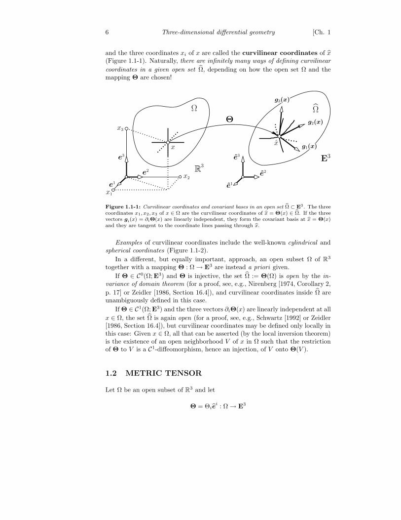
and the three coordinates xi of x are called the curvilinear coordinates of x(Figure 1.1-1). Naturally, there are infinitely many ways of defining curvilinear
coordinates in a given open set Ω, depending on how the open set Ω and themapping Θ are chosen!
Ω
x
x3
x1
x2
e2
e3
e1
R3
Θ
e2
e3
e1
x
Ω
g2(x)
g3(x)
g1(x)
E3
Figure 1.1-1: Curvilinear coordinates and covariant bases in an open set bΩ ⊂ E3. The threecoordinates x1, x2, x3 of x ∈ Ω are the curvilinear coordinates of bx = Θ(x) ∈ bΩ. If the threevectors gi(x) = ∂iΘ(x) are linearly independent, they form the covariant basis at bx = Θ(x)and they are tangent to the coordinate lines passing through bx.
Examples of curvilinear coordinates include the well-known cylindrical andspherical coordinates (Figure 1.1-2).
In a different, but equally important, approach, an open subset Ω of R3
together with a mapping Θ : Ω → E3 are instead a priori given.
If Θ ∈ C0(Ω;E3) and Θ is injective, the set Ω := Θ(Ω) is open by the in-
variance of domain theorem (for a proof, see, e.g., Nirenberg [1974, Corollary 2,
p. 17] or Zeidler [1986, Section 16.4]), and curvilinear coordinates inside Ω areunambiguously defined in this case.
If Θ ∈ C1(Ω;E3) and the three vectors ∂iΘ(x) are linearly independent at all
x ∈ Ω, the set Ω is again open (for a proof, see, e.g., Schwartz [1992] or Zeidler[1986, Section 16.4]), but curvilinear coordinates may be defined only locally inthis case: Given x ∈ Ω, all that can be asserted (by the local inversion theorem)is the existence of an open neighborhood V of x in Ω such that the restrictionof Θ to V is a C1-diffeomorphism, hence an injection, of V onto Θ(V ).
1.2 METRIC TENSOR
Let Ω be an open subset of R3 and let
Θ = Θiei : Ω → E3
Sect. 1.2] Metric tensor 7
ρ
z
x
ϕ
Ω
E3
r
x
ϕ
Ω
E3ψ
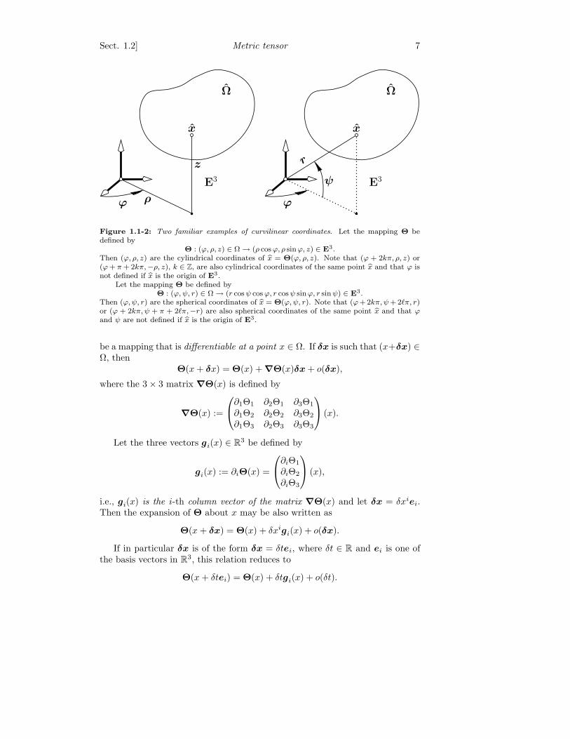
Figure 1.1-2: Two familiar examples of curvilinear coordinates. Let the mapping Θ bedefined by
Θ : (ϕ, ρ, z) ∈ Ω → (ρ cosϕ, ρ sinϕ, z) ∈ E3.Then (ϕ, ρ, z) are the cylindrical coordinates of bx = Θ(ϕ, ρ, z). Note that (ϕ + 2kπ, ρ, z) or(ϕ+ π+ 2kπ,−ρ, z), k ∈ Z, are also cylindrical coordinates of the same point bx and that ϕ isnot defined if bx is the origin of E3.
Let the mapping Θ be defined byΘ : (ϕ, ψ, r) ∈ Ω → (r cosψ cosϕ, r cosψ sinϕ, r sinψ) ∈ E3.
Then (ϕ,ψ, r) are the spherical coordinates of bx = Θ(ϕ, ψ, r). Note that (ϕ+2kπ,ψ+2`π, r)or (ϕ + 2kπ,ψ + π + 2`π,−r) are also spherical coordinates of the same point bx and that ϕand ψ are not defined if bx is the origin of E3.
be a mapping that is differentiable at a point x ∈ Ω. If δx is such that (x+δx) ∈Ω, then
Θ(x + δx) = Θ(x) + ∇Θ(x)δx+ o(δx),
where the 3 × 3 matrix ∇Θ(x) is defined by
∇Θ(x) :=
∂1Θ1 ∂2Θ1 ∂3Θ1
∂1Θ2 ∂2Θ2 ∂3Θ2
∂1Θ3 ∂2Θ3 ∂3Θ3
(x).
Let the three vectors gi(x) ∈ R3 be defined by
gi(x) := ∂iΘ(x) =
∂iΘ1
∂iΘ2
∂iΘ3
(x),
i.e., gi(x) is the i-th column vector of the matrix ∇Θ(x) and let δx = δxiei.Then the expansion of Θ about x may be also written as
Θ(x + δx) = Θ(x) + δxigi(x) + o(δx).
If in particular δx is of the form δx = δtei, where δt ∈ R and ei is one ofthe basis vectors in R3, this relation reduces to
Θ(x + δtei) = Θ(x) + δtgi(x) + o(δt).

8 Three-dimensional differential geometry [Ch. 1
A mapping Θ : Ω → E3 is an immersion at x ∈ Ω if it is differentiableat x and the matrix ∇Θ(x) is invertible or, equivalently, if the three vectorsgi(x) = ∂iΘ(x) are linearly independent.
Assume from now on in this section that the mapping Θ is an immersion
at x. Then the three vectors gi(x) constitute the covariant basis at the pointx = Θ(x).
In this case, the last relation thus shows that each vector gi(x) is tangent
to the i-th coordinate line passing through x = Θ(x), defined as the image
by Θ of the points of Ω that lie on the line parallel to ei passing through x(there exist t0 and t1 with t0 < 0 < t1 such that the i-th coordinate line isgiven by t ∈ ]t0, t1[ → f i(t) := Θ(x + tei) in a neighborhood of x; hencef ′
i(0) = ∂iΘ(x) = gi(x)); see Figures 1.1-1 and 1.1-2.Returning to a general increment δx = δxiei, we also infer from the expan-
sion of Θ about x that (recall that we use the summation convention):
|Θ(x + δx) −Θ(x)|2 = δxT∇Θ(x)T
∇Θ(x)δx+ o(|δx|2
)
= δxigi(x) · gj(x)δxj + o(|δx|2
).
In other words, the principal part with respect to δx of the length betweenthe points Θ(x + δx) and Θ(x) is δxigi(x) · gj(x)δxj1/2. This observationsuggests to define a matrix (gij(x)) of order three, by letting
gij(x) := gi(x) · gj(x) = (∇Θ(x)T∇Θ(x))ij .
The elements gij(x) of this symmetric matrix are called the covariant com-
ponents of the metric tensor at x = Θ(x).Note that the matrix ∇Θ(x) is invertible and that the matrix (gij(x)) is
positive definite, since the vectors gi(x) are assumed to be linearly independent.The three vectors gi(x) being linearly independent, the nine relations
gi(x) · gj(x) = δij
unambiguously define three linearly independent vectors gi(x). To see this, leta priori gi(x) = X ik(x)gk(x) in the relations gi(x) · gj(x) = δi
j . This gives
X ik(x)gkj(x) = δij ; consequently, X ik(x) = gik(x), where
(gij(x)) := (gij(x))−1.
Hence gi(x) = gik(x)gk(x). These relations in turn imply that
gi(x) · gj(x) =(gik(x)gk(x)
)·(gj`(x)g`(x)
)
= gik(x)gj`(x)gk`(x) = gik(x)δjk = gij(x),
and thus the vectors gi(x) are linearly independent since the matrix (gij(x)) ispositive definite. We would likewise establish that gi(x) = gij(x)gj(x).
The three vectors gi(x) form the contravariant basis at the point x = Θ(x)and the elements gij(x) of the symmetric positive definite matrix (gij(x)) arethe contravariant components of the metric tensor at x = Θ(x).
Sect. 1.3] Volumes, areas, and lengths in curvilinear coordinates 9
To conclude this section, we record for convenience the fundamental relationsthat exist between the vectors of the covariant and contravariant bases and thecovariant and contravariant components of the metric tensor:
gij(x) = gi(x) · gj(x) and gij(x) = gi(x) · gj(x),
gi(x) = gij(x)gj(x) and gi(x) = gij(x)gj(x).
1.3 VOLUMES, AREAS, AND LENGTHS IN CURVI-
LINEAR COORDINATES
We now review fundamental formulas showing how volume, area, and length
elements at a point x = Θ(x) in the set Ω = Θ(Ω) can be expressed either interms of the matrix ∇Θ(x) or in terms of the matrix (gij(x)) or of its inversematrix (gij(x)).
These formulas thus highlight the crucial role played by the matrix (gij(x))for computing “metric” notions at the point x = Θ(x). Indeed, the “metrictensor” well deserves its name!
A domain in Rn is a bounded, open, and connected subset D of R3 witha Lipschitz-continuous boundary, the set D being locally on one side of itsboundary. All relevant details needed here about domains are found in Necas[1967] or Adams [1975].
Given a domain D ⊂ R3 with boundary Γ, we let dx denote the volume
element in D, dΓ denote the area element along Γ, and n = niei denote the
unit (|n| = 1) outer normal vector along Γ (dΓ is well defined and n is defineddΓ-almost everywhere since Γ is assumed to be Lipschitz-continuous).
Note also that the assumptions made on the mapping Θ in the next theoremguarantee that, if D is a domain in R3 such that D ⊂ Ω, then D− ⊂ Ω,
Θ(D)− = Θ(D), and the boundaries ∂D of D and ∂D of D are related by
∂D = Θ(∂D) (see, e.g., Ciarlet [1988, Theorem 1.2-8 and Example 1.7]).If A is a square matrix, CofA denotes the cofactor matrix of A. Thus
CofA = (det A)A−T if A is invertible.A mapping Θ : Ω → E3 is an immersion if it is an immersion at each
x ∈ Ω, i.e., if Θ is differentiable in Ω and the three vectors gi(x) = ∂iΘ(x) arelinearly independent at each x ∈ Ω.
Theorem 1.3-1. Let Ω be an open subset of R3, let Θ : Ω → E3 be an injective
and smooth enough immersion, and let Ω = Θ(Ω).
(a) The volume element dx at x = Θ(x) ∈ Ω is given in terms of the volume
element dx at x ∈ Ω by
dx = | det ∇Θ(x)|dx =√
g(x)dx, where g(x) := det(gij(x)).
(b) Let D be a domain in R3 such that D ⊂ Ω. The area element dΓ(x) at
x = Θ(x) ∈ ∂D is given in terms of the area element dΓ(x) at x ∈ ∂D by
dΓ(x) = |Cof∇Θ(x)n(x)|dΓ(x) =√
g(x)√
ni(x)gij(x)nj(x)dΓ(x),
10 Three-dimensional differential geometry [Ch. 1
where n(x) := ni(x)ei denotes the unit outer normal vector at x ∈ ∂D.
(c) The length element d(x) at x = Θ(x) ∈ Ω is given by
d(x) =δxT
∇Θ(x)T∇Θ(x)δx
1/2=
δxigij(x)δxj
1/2,
where δx = δxiei.
Proof. The relation dx = | det ∇Θ(x)| dx between the volume elementsis well known. The second relation in (a) follows from the relation g(x) =| det ∇Θ(x)|2, which itself follows from the relation (gij(x)) = ∇Θ(x)T ∇Θ(x).
Indications about the proof of the relation between the area elements dΓ(x)and dΓ(x) given in (b) are found in Ciarlet [1988, Theorem 1.7-1] (in this for-mula, n(x) = ni(x)ei is identified with the column vector in R3 with ni(x) asits components). Using the relations Cof (AT ) = (CofA)T and Cof(AB) =(CofA)(CofB), we next have:
|Cof∇Θ(x)n(x)|2 = n(x)T Cof(∇Θ(x)T
∇Θ(x))n(x)
= g(x)ni(x)gij(x)nj(x).
Either expression of the length element given in (c) recalls that d(x) isby definition the principal part with respect to δx = δxiei of the length|Θ(x + δx) − Θ(x)|, whose expression precisely led to the introduction of thematrix (gij(x)) in Section 1.2.
The relations found in Theorem 1.3-1 are used in particular for computingvolumes, areas, and lengths inside Ω by means of integrals inside Ω, i.e., in termsof the curvilinear coordinates used in the open set Ω (Figure 1.3-1):
Let D be a domain in R3 such that D ⊂ Ω, let D := Θ(D), and let f ∈ L1(D)be given. Then ∫
bDf(x)dx =
∫
D
(f Θ)(x)√
g(x)dx.
In particular, the volume of D is given by
vol D :=
∫
bDdx =
∫
D
√g(x)dx.
Next, let Γ := ∂D, let Σ be a dΓ-measurable subset of Γ, let Σ := Θ(Σ) ⊂∂D, and let h ∈ L1(Σ) be given. Then
∫
bΣh(x)dΓ(x) =
∫
Σ
(h Θ)(x)√
g(x)√
ni(x)gij(x)nj(x)dΓ(x).
In particular, the area of Σ is given by
area Σ :=
∫
bΣdΓ(x) =
∫
Σ
√g(x)
√ni(x)gij(x)nj(x)dΓ(x).
Sect. 1.4] Covariant derivatives and Christoffel symbols 11
t
x Θ(x) = x
x+δx Θ(x+δx)
I R
f
C
Θ
C
ΩA
dΓ(x)
n(x)
V
dx
Ω
dl(x)
dΓ(x)
A
V
dx
R3
E3
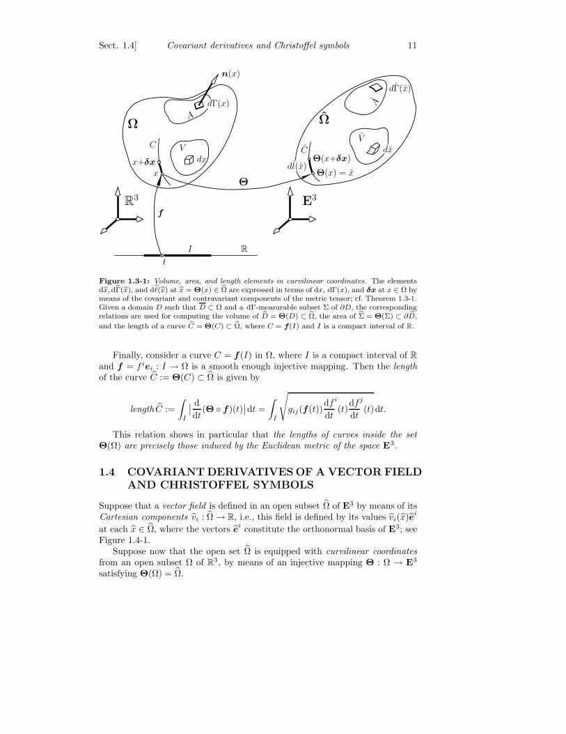
Figure 1.3-1: Volume, area, and length elements in curvilinear coordinates. The elementsdbx,dbΓ(bx), and db(bx) at bx = Θ(x) ∈ bΩ are expressed in terms of dx, dΓ(x), and δx at x ∈ Ω bymeans of the covariant and contravariant components of the metric tensor; cf. Theorem 1.3-1.Given a domain D such that D ⊂ Ω and a dΓ-measurable subset Σ of ∂D, the correspondingrelations are used for computing the volume of bD = Θ(D) ⊂ bΩ, the area of bΣ = Θ(Σ) ⊂ ∂ bD,
and the length of a curve bC = Θ(C) ⊂ bΩ, where C = f(I) and I is a compact interval of R.
Finally, consider a curve C = f(I) in Ω, where I is a compact interval of R
and f = f iei : I → Ω is a smooth enough injective mapping. Then the length
of the curve C := Θ(C) ⊂ Ω is given by
length C :=
∫
I
∣∣ d
dt(Θ f)(t)
∣∣dt =
∫
I
√
gij(f(t))df
dt
i
(t)df
dt
j
(t)dt.
This relation shows in particular that the lengths of curves inside the set
Θ(Ω) are precisely those induced by the Euclidean metric of the space E3.
1.4 COVARIANT DERIVATIVES OF A VECTOR FIELD
AND CHRISTOFFEL SYMBOLS
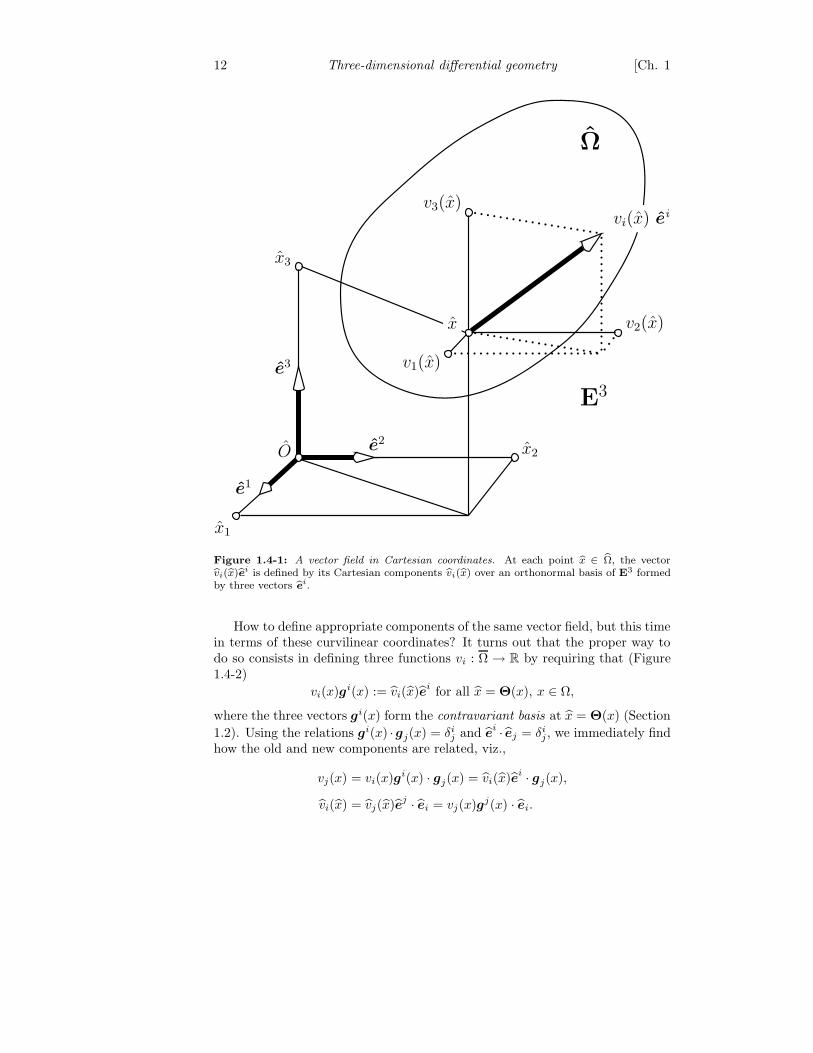
Suppose that a vector field is defined in an open subset Ω of E3 by means of itsCartesian components vi : Ω → R, i.e., this field is defined by its values vi(x)ei
at each x ∈ Ω, where the vectors ei constitute the orthonormal basis of E3; seeFigure 1.4-1.
Suppose now that the open set Ω is equipped with curvilinear coordinates
from an open subset Ω of R3, by means of an injective mapping Θ : Ω → E3
satisfying Θ(Ω) = Ω.
12 Three-dimensional differential geometry [Ch. 1
x1
x2O
x3
v1(x)
v2(x)
v3(x)
e1
e2
e3
E3
Ω
vi(x) ei
x
Figure 1.4-1: A vector field in Cartesian coordinates. At each point bx ∈ bΩ, the vectorbvi(bx)bei is defined by its Cartesian components bvi(bx) over an orthonormal basis of E3 formedby three vectors bei.
How to define appropriate components of the same vector field, but this timein terms of these curvilinear coordinates? It turns out that the proper way todo so consists in defining three functions vi : Ω → R by requiring that (Figure1.4-2)
vi(x)gi(x) := vi(x)ei for all x = Θ(x), x ∈ Ω,
where the three vectors gi(x) form the contravariant basis at x = Θ(x) (Section
1.2). Using the relations gi(x) ·gj(x) = δij and ei · ej = δi
j , we immediately findhow the old and new components are related, viz.,
vj(x) = vi(x)gi(x) · gj(x) = vi(x)ei · gj(x),
vi(x) = vj(x)ej · ei = vj(x)gj(x) · ei.
Sect. 1.4] Covariant derivatives and Christoffel symbols 13
x1
x2
x3
x
e1
e2
e3
ΩR
3
Θ
e1
e2
e3 g1(x)
g2(x)
ui(x)gi(x)
g3(x)
u3(x)
u2(x)
u1(x)x
ΩE3
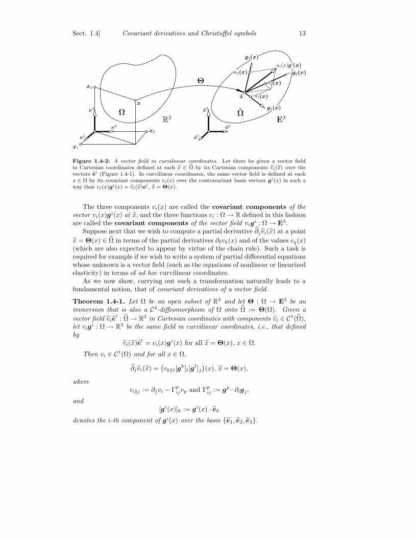
Figure 1.4-2: A vector field in curvilinear coordinates. Let there be given a vector fieldin Cartesian coordinates defined at each bx ∈ bΩ by its Cartesian components bvi(bx) over thevectors bei (Figure 1.4-1). In curvilinear coordinates, the same vector field is defined at eachx ∈ Ω by its covariant components vi(x) over the contravariant basis vectors gi(x) in such away that vi(x)g
i(x) = bvi(bx)ei, bx = Θ(x).
The three components vi(x) are called the covariant components of the
vector vi(x)gi(x) at x, and the three functions vi : Ω → R defined in this fashionare called the covariant components of the vector field vig
i : Ω → E3.Suppose next that we wish to compute a partial derivative ∂j vi(x) at a point
x = Θ(x) ∈ Ω in terms of the partial derivatives ∂`vk(x) and of the values vq(x)(which are also expected to appear by virtue of the chain rule). Such a task isrequired for example if we wish to write a system of partial differential equationswhose unknown is a vector field (such as the equations of nonlinear or linearizedelasticity) in terms of ad hoc curvilinear coordinates.
As we now show, carrying out such a transformation naturally leads to afundamental notion, that of covariant derivatives of a vector field.
Theorem 1.4-1. Let Ω be an open subset of R3 and let Θ : Ω → E3 be an
immersion that is also a C2-diffeomorphism of Ω onto Ω := Θ(Ω). Given a
vector field viei : Ω → R
3 in Cartesian coordinates with components vi ∈ C1(Ω),let vig
i : Ω → R3 be the same field in curvilinear coordinates, i.e., that defined
by
vi(x)ei = vi(x)gi(x) for all x = Θ(x), x ∈ Ω.
Then vi ∈ C1(Ω) and for all x ∈ Ω,
∂j vi(x) =(vk‖`[g
k]i[g`]j
)(x), x = Θ(x),
where
vi‖j := ∂jvi − Γpijvp and Γp
ij := gp · ∂igj ,
and
[gi(x)]k := gi(x) · ek
denotes the i-th component of gi(x) over the basis e1, e2, e3.
14 Three-dimensional differential geometry [Ch. 1
Proof. The following convention holds throughout this proof: The simul-taneous appearance of x and x in an equality means that they are related byx = Θ(x) and that the equality in question holds for all x ∈ Ω.
(i) Another expression of [gi(x)]k := gi(x) · ek.
Let Θ(x) = Θk(x)ek and Θ(x) = Θi(x)ei, where Θ : Ω → E3 denotes the
inverse mapping of Θ : Ω → E3. Since Θ(Θ(x)) = x for all x ∈ Ω, the chainrule shows that the matrices ∇Θ(x) := (∂jΘ
k(x)) (the row index is k) and
∇Θ(x) := (∂kΘi(x)) (the row index is i) satisfy
∇Θ(x)∇Θ(x) = I,
or equivalently,
∂kΘi(x)∂jΘk(x) =
(∂1Θ
i(x) ∂2Θi(x) ∂3Θ
i(x))
∂jΘ1(x)
∂jΘ2(x)
∂jΘ3(x)
= δi
j .
The components of the above column vector being precisely those of thevector gj(x), the components of the above row vector must be those of the
vector gi(x) since gi(x) is uniquely defined for each exponent i by the threerelations gi(x) · gj(x) = δi
j , j = 1, 2, 3. Hence the k-th component of gi(x) over
the basis e1, e2, e3 can be also expressed in terms of the inverse mapping Θ,as:
[gi(x)]k = ∂kΘi(x).
(ii) The functions Γq`k := gq · ∂`gk ∈ C0(Ω).
We next compute the derivatives ∂`gq(x) (the fields gq = gqrgr are of class
C1 on Ω since Θ is assumed to be of class C2). These derivatives will be needed
in (iii) for expressing the derivatives ∂j ui(x) as functions of x (recall that ui(x) =uk(x)[gk(x)]i). Recalling that the vectors gk(x) form a basis, we may write a
priori
∂`gq(x) = −Γq
`k(x)gk(x),
thereby unambiguously defining functions Γq`k : Ω → R. To find their expres-
sions in terms of the mappings Θ and Θ, we observe that
Γq`k(x) = Γq
`m(x)δmk = Γq
`m(x)gm(x) · gk(x) = −∂`gq(x) · gk(x).
Hence, noting that ∂`(gq(x) · gk(x)) = 0 and [gq(x)]p = ∂pΘ
q(x), we obtain
Γq`k(x) = gq(x) · ∂`gk(x) = ∂pΘ
q(x)∂`kΘp(x) = Γqk`(x).
Since Θ ∈ C2(Ω;E3) and Θ ∈ C1(Ω; R3) by assumption, the last relationsshow that Γq
`k ∈ C0(Ω).

Sect. 1.4] Covariant derivatives and Christoffel symbols 15
(iii) The partial derivatives ∂ivi(x) of the Cartesian components of the vector
field viei ∈ C1(Ω; R3) are given at each x = Θ(x) ∈ Ω by
∂j vi(x) = vk‖`(x)[gk(x)]i[g`(x)]j ,
where
vk‖`(x) := ∂`vk(x) − Γq`k(x)vq(x),
and [gk(x)]i and Γq`k(x) are defined as in (i) and (ii).
We compute the partial derivatives ∂j vi(x) as functions of x by means of therelation vi(x) = vk(x)[gk(x)]i. To this end, we first note that a differentiablefunction w : Ω → R satisfies
∂jw(Θ(x)) = ∂`w(x)∂j Θ`(x) = ∂`w(x)[g`(x)]j ,
by the chain rule and by (i). In particular then,
∂j vi(x) = ∂jvk(Θ(x))[gk(x)]i + vq(x)∂j [gq(Θ(x))]i
= ∂`vk(x)[g`(x)]j [gk(x)]i + vq(x)
(∂`[g
q(x)]i)[g`(x)]j
= (∂`vk(x) − Γq`k(x)vq(x)) [gk(x)]i[g
`(x)]j ,
since ∂`gq(x) = −Γq
`k(x)gk(x) by (ii).
The functionsvi‖j = ∂jvi − Γp
ijvp
defined in Theorem 1.4-1 are called the first-order covariant derivatives ofthe vector field vig
i : Ω → R3.The functions
Γpij = gp · ∂igj
are called the Christoffel symbols of the first kind.The following result summarizes properties of covariant derivatives and Christof-
fel symbols that are constantly used.
Theorem 1.4-2. Let the assumptions on the mapping Θ : Ω → E3 be as in
Theorem 1.4-1, and let there be given a vector field vigi : Ω → R3 with covariant
components vi ∈ C1(Ω).(a) The first-order covariant derivatives vi‖j ∈ C0(Ω) of the vector field
vigi : Ω → R3, which are defined by
vi‖j := ∂jvi − Γpijvp, where Γp
ij := gp · ∂igj ,
can be also defined by the relations
∂j(vigi) = vi‖jg
i ⇐⇒ vi‖j =∂j(vkg
k)· gi.
(b) The Christoffel symbols Γpij := gp·∂igj = Γp
ji ∈ C0(Ω) satisfy the relations
∂igp = −Γp
ijgj and ∂jgq = Γi
jqgi.
16 Three-dimensional differential geometry [Ch. 1
Proof. It remains to verify that the covariant derivatives vi‖j , defined inTheorem 1.4-1 by
vi‖j = ∂jvi − Γpijvp,
may be equivalently defined by the relations
∂j(vigi) = vi‖jg
i.
These relations unambiguously define the functions vi‖j = ∂j(vkgk) · gi since
the vectors gi are linearly independent at all points of Ω by assumption. Tothis end, we simply note that, by definition, the Christoffel symbols satisfy∂ig
p = −Γpijg
j (cf. part (ii) of the proof of Theorem 1.4-1); hence
∂j(vigi) = (∂jvi)g
i + vi∂jgi = (∂jvi)g
i − viΓijkg
k = vi‖jgi.
To establish the other relations ∂jgq = Γijqgi, we note that
0 = ∂j(gp · gq) = −Γp
jigi · gq + gp · ∂jgq = −Γp
qj + gp · ∂jgq .
Hence∂jgq = (∂jgq · gp)gp = Γp
qjgp.
Remark. The Christoffel symbols Γpij can be also defined solely in terms of
the components of the metric tensor; see the proof of Theorem 1.5-1.
If the affine space E3 is identified with R3 and Θ = idΩ, the relation∂j(vig
i)(x) = (vi‖jgi)(x) (Theorem 1.4-2 (a)), reduces to ∂j(vi(x)ei) = (∂j vi(x))ei.
In this sense, a covariant derivative of the first order constitutes a generalization
of a partial derivative of the first order in Cartesian coordinates.
1.5 NECESSARY CONDITIONS SATISFIED BY THE
METRIC TENSOR; THE RIEMANN CURVATURE
TENSOR
It is remarkable that the components gij : Ω → R of the metric tensor of an
open set Θ(Ω) ⊂ E3 (Section 1.2), defined by a smooth enough immersionΘ : Ω → E3, cannot be arbitrary functions.
As shown in the next theorem, they must satisfy relations that take theform:
∂jΓikq − ∂kΓijq + ΓpijΓkqp − Γp
ikΓjqp = 0 in Ω,
where the functions Γijq and Γpij have simple expressions in terms of the func-
tions gij and of some of their partial derivatives (as shown in the next proof,it so happens that the functions Γp
ij as defined in Theorem 1.5-1 coincide withthe Christoffel symbols introduced in the previous section; this explains why
Sect. 1.5] Necessary conditions satisfied by the metric tensor 17
they are denoted by the same symbol). Note that, according to the rule gov-erning Latin indices and exponents, these relations are meant to hold for alli, j, k, q ∈ 1, 2, 3.
Theorem 1.5-1. Let Ω be an open set in R3, let Θ ∈ C3(Ω;E3) be an immer-
sion, and let
gij := ∂iΘ · ∂jΘ
denote the covariant components of the metric tensor of the set Θ(Ω). Let the
functions Γijq ∈ C1(Ω) and Γpij ∈ C1(Ω) be defined by
Γijq :=1
2(∂jgiq + ∂igjq − ∂qgij),
Γpij := gpqΓijq where (gpq) := (gij)
−1.
Then, necessarily,
∂jΓikq − ∂kΓijq + ΓpijΓkqp − Γp
ikΓjqp = 0 in Ω.
Proof. Let gi = ∂iΘ. It is then immediately verified that the functions Γijq
are also given by
Γijq = ∂igj · gq .
For each x ∈ Ω, let the three vectors gj(x) be defined by the relations gj(x) ·gi(x) = δj
j . Since we also have gj = gijgi, the last relations imply that Γpij =
∂igj · gp. Therefore,∂igj = Γp
ijgp
since ∂igj = (∂igj · gp)gp. Differentiating the same relations yields
∂kΓijq = ∂ikgj · gq + ∂igj · ∂kgq ,
so that the above relations together give
∂igj · ∂kgq = Γpijgp · ∂kgq = Γp
ijΓkqp.
Consequently,∂ikgj · gq = ∂kΓijq − Γp
ijΓkqp.
Since ∂ikgj = ∂ijgk, we also have
∂ikgj · gq = ∂jΓikq − ΓpikΓjqp,
and thus the required necessary conditions immediately follow.
Remark. The vectors gi and gj introduced above form the covariant andcontravariant bases and the functions gij are the contravariant components ofthe metric tensor (Section 1.2).
18 Three-dimensional differential geometry [Ch. 1
As shown in the above proof, the necessary conditions Rqijk = 0 thus sim-ply constitute a re-writing of the relations ∂ikgj = ∂kigj in the form of theequivalent relations ∂ikgj · gq = ∂kigj · gq .
The functions
Γijq =1
2(∂jgiq + ∂igjq − ∂qgij) = ∂igj · gq = Γjiq
andΓp
ij = gpqΓijq = ∂igj · gp = Γpji
are the Christoffel symbols of the first, and second, kinds. We saw inSection 1.4 that the same Christoffel symbols Γp
ij also naturally appear in adifferent context (that of covariant differentiation).
Finally, the functions
Rqijk := ∂jΓikq − ∂kΓijq + ΓpijΓkqp − Γp
ikΓjqp
are the covariant components of the Riemann curvature tensor of theset Θ(Ω). The relations Rqijk = 0 found in Theorem 1.4-1 thus express thatthe Riemann curvature tensor of the set Θ(Ω) (equipped with the metric tensorwith covariant components gij) vanishes.
1.6 EXISTENCE OF AN IMMERSION DEFINED ON
AN OPEN SET IN R3 WITH A PRESCRIBED MET-
RIC TENSOR
Let M3, S3, and S
3> denote the sets of all square matrices of order three, of
all symmetric matrices of order three, and of all symmetric positive definitematrices of order three.
As in Section 1.2, the matrix representing the Frechet derivative at x ∈ Ω ofa differentiable mapping Θ = (Θ`) : Ω → E3 is denoted
∇Θ(x) := (∂jΘ`(x)) ∈ M3,
where ` is the row index and j the column index (equivalently, ∇Θ(x) is thematrix of order three whose j-th column vector is ∂jΘ).
So far, we have considered that we are given an open set Ω ⊂ R3 and asmooth enough immersion Θ : Ω → E3, thus allowing us to define a matrix field
C = (gij) = ∇ΘT∇Θ : Ω → S
3>,
where gij : Ω → R are the covariant components of the metric tensor of theopen set Θ(Ω) ⊂ E3.
We now turn to the reciprocal questions :Given an open subset Ω of R3 and a smooth enough matrix field C = (gij) :
Ω → S3>, when is C the metric tensor field of an open set Θ(Ω) ⊂ E3? Equiva-
lently, when does there exist an immersion Θ : Ω → E3 such that
C = ∇ΘT∇Θ in Ω,

Sect. 1.6] Existence of an immersion with a prescribed metric tensor 19
or equivalently, such that
gij = ∂iΘ · ∂jΘ in Ω?
If such an immersion exists, to what extent is it unique?The answers to these questions turn out to be remarkably simple: If Ω is
simply-connected, the necessary conditions
∂jΓikq − ∂kΓijq + ΓpijΓkqp − Γp
ikΓjqp = 0 in Ω
found in Theorem 1.4-1 are also sufficient for the existence of such an immer-
sion. If Ω is connected, this immersion is unique up to isometries in E3.
Whether the immersion found in this fashion is globally injective is a differentissue, which accordingly should be resolved by different means.
This result comprises two essentially distinct parts, a global existence result
(Theorem 1.6-1) and a uniqueness result (Theorem 1.4-1). Note that these tworesults are established under different assumptions on the set Ω and on thesmoothness of the field (gij).
In order to put these results in a wider perspective, let us make a briefincursion into Riemannian Geometry. For detailed treatments, see classic textssuch as Choquet-Bruhat, de Witt-Morette & Dillard-Bleick [1977], Marsden &Hughes [1983], or Gallot, Hulin & Lafontaine [2004].
Considered as a three-dimensional manifold, an open set Ω ⊂ R3 equippedwith an immersion Θ : Ω → E3 becomes an example of a Riemannian manifold
(Ω; (gij)), i.e., a manifold, the set Ω, equipped with a Riemannian metric, thesymmetric positive-definite matrix field (gij) : Ω → S3
> defined in this case bygij := ∂iΘ · ∂jΘ in Ω. More generally, a Riemannian metric on a manifold
is a twice covariant, symmetric, positive-definite tensor field acting on vectorsin the tangent spaces to the manifold (these tangent spaces coincide with R
3 inthe present instance).
This particular Riemannian manifold (Ω; (gij)) possesses the remarkableproperty that its metric is the same as that of the surrounding space E3. Morespecifically, (Ω; (gij)) is isometrically immersed in the Euclidean space E3,in the sense that there exists an immersion Θ : Ω → E3 that satisfies the rela-tions gij = ∂iΘ · ∂jΘ. Equivalently, the length of any curve in the Riemannianmanifold (Ω; (gij)) is the same as the length of its image by Θ in the Euclideanspace E3 (see Theorem 1.3-1).
The first question above can thus be rephrased as follows: Given an open
subset Ω of R3 and a positive-definite matrix field (gij) : Ω → S3>, when is
the Riemannian manifold (Ω; (gij)) flat, in the sense that it can be locallyisometrically immersed in a Euclidean space of the same dimension (three)?
The answer to this question can then be rephrased as follows (compare withthe statement of Theorem 1.6-1 below): Let Ω be a simply-connected open subset
of R3. Then a Riemannian manifold (Ω; (gij)) with a Riemannian metric (gij)of class C2 in Ω is flat if and only if its Riemannian curvature tensor vanishes
in Ω. Recast as such, this result becomes a special case of the fundamental
theorem on flat Riemannian manifolds, which holds for a general finite-dimensional Riemannian manifold.
20 Three-dimensional differential geometry [Ch. 1
The answer to the second question, viz., the issue of uniqueness, can berephrased as follows (compare with the statement of Theorem 1.7-1 in the nextsection): Let Ω be a connected open subset of R
3. Then the isometric immersions
of a flat Riemannian manifold (Ω; (gij)) into a Euclidean space E3 are unique
up to isometries of E3. Recast as such, this result likewise becomes a specialcase of the so-called rigidity theorem; cf. Section 1.7.
Recast as such, these two theorems together constitute a special case (thatwhere the dimensions of the manifold and of the Euclidean space are both equalto three) of the fundamental theorem of Riemannian Geometry. Thistheorem addresses the same existence and uniqueness questions in the moregeneral setting where Ω is replaced by a p-dimensional manifold and E3 is re-placed by a (p + q)-dimensional Euclidean space (the “fundamental theorem ofsurface theory”, established in Sections 2.8 and 2.9, constitutes another impor-tant special case). When the p-dimensional manifold is an open subset of Rp,an outline of a self-contained proof is given in Szopos [2005].
Another fascinating question (which will not be addressed here) is the follow-ing: Given again an open subset Ω of R3 equipped with a symmetric, positive-definite matrix field (gij) : Ω → S
3, assume this time that the Riemannian
manifold (Ω; (gij)) is no longer flat, i.e., its Riemannian curvature tensor nolonger vanishes in Ω. Can such a Riemannian manifold still be isometrically
immersed, but this time in a higher-dimensional Euclidean space? Equivalently,do there exist a Euclidean space Ed with d > 3 and an immersion Θ : Ω → Ed
such that gij = ∂iΘ · ∂jΘ in Ω?
The answer is yes, according to the following beautiful Nash theorem, sonamed after Nash [1954]: Any p-dimensional Riemannian manifold equipped
with a continuous metric can be isometrically immersed in a Euclidean space
of dimension 2p with an immersion of class C1; it can also be isometrically
immersed in a Euclidean space of dimension (2p + 1) with a globally injective
immersion of class C1.
Let us now humbly return to the question of existence raised at the beginningof this section, i.e., when the manifold is an open set in R3.
Theorem 1.6-1. Let Ω be a connected and simply-connected open set in R3
and let C = (gij) ∈ C2(Ω; S3>) be a matrix field that satisfies
Rqijk := ∂jΓikq − ∂kΓijq + ΓpijΓkqp − Γp
ikΓjqp = 0 in Ω,
where
Γijq :=1
2(∂jgiq + ∂igjq − ∂qgij),
Γpij := gpqΓijq with (gpq) := (gij)
−1.
Then there exists an immersion Θ ∈ C3(Ω;E3) such that
C = ∇ΘT∇Θ in Ω.

Sect. 1.6] Existence of an immersion with a prescribed metric tensor 21
Proof. The proof relies on a simple, yet crucial, observation. When a smoothenough immersion Θ = (Θ`) : Ω → E3 is a priori given (as it was so far), itscomponents Θ` satisfy the relations ∂ijΘ` = Γp
ij∂pΘ`, which are nothing butanother way of writing the relations ∂igj = Γp
ijgp (see the proof of Theorem1.5-1). This observation thus suggests to begin by solving (see part (ii)) thesystem of partial differential equations
∂iF`j = ΓpijF`p in Ω,
whose solutions F`j : Ω → R then constitute natural candidates for the partialderivatives ∂jΘ` of the unknown immersion Θ = (Θ`) : Ω → E3 (see part (iii)).
To begin with, we establish in (i) relations that will in turn allow us tore-write the sufficient conditions
∂jΓikq − ∂kΓijq + ΓpijΓkqp − Γp
ikΓjqp = 0 in Ω
in a slightly different form, more appropriate for the existence result of part (ii).Note that the positive definiteness of the symmetric matrices (gij) is not neededfor this purpose.
(i) Let Ω be an open subset of R3 and let there be given a field (gij) ∈C2(Ω; S3) of symmetric invertible matrices. The functions Γijq , Γ
pij , and gpq
being defined by
Γijq :=1
2(∂jgiq + ∂igjq − ∂qgij), Γp
ij := gpqΓijq , (gpq) := (gij)−1,
define the functions
Rqijk := ∂jΓikq − ∂kΓijq + ΓpijΓkqp − Γp
ikΓjqp,
Rp·ijk := ∂jΓ
pik − ∂kΓp
ij + Γ`ikΓp
j` − Γ`ijΓ
pk`.
Then
Rp·ijk = gpqRqijk and Rqijk = gpqR
p·ijk .
Using the relations
Γjq` + Γ`jq = ∂jgq` and Γikq = gq`Γ`ik,
which themselves follow from the definitions of the functions Γijq and Γpij , and
noting that(gpq∂jgq` + gq`∂jg
pq) = ∂j(gpqgq`) = 0,
we obtain
gpq(∂jΓikq − ΓrikΓjqr) = ∂jΓ
pik − Γikq∂jg
pq − Γ`ikgpq(∂jgq` − Γ`jq)
= ∂jΓpik + Γ`
ikΓpj` − Γ`
ik(gpq∂jgq` + gq`∂jgpq)
= ∂jΓpik + Γ`
ikΓpj`.

22 Three-dimensional differential geometry [Ch. 1
Likewise,gpq(∂kΓijq − Γr
ijΓkqr) = ∂kΓpij − Γ`
ijΓpk`,
and thus the relations Rp·ijk = gpqRqijk are established. The relations Rqijk =
gpqRp·ijk are clearly equivalent to these ones.
We next establish the existence of solutions to the system
∂iF`j = ΓpijF`p in Ω.
(ii) Let Ω be a connected and simply-connected open subset of R3 and let
there be given functions Γpij = Γp
ji ∈ C1(Ω) satisfying the relations
∂jΓpik − ∂kΓp
ij + Γ`ikΓp
j` − Γ`ijΓ
pk` = 0 in Ω,
which are equivalent to the relations
∂jΓikq − ∂kΓijq + ΓpijΓkqp − Γp
ikΓjqp = 0 in Ω,
by part (i).Let a point x0 ∈ Ω and a matrix (F 0
`j) ∈ M3 be given. Then there exists one,
and only one, field (F`j) ∈ C2(Ω; M3) that satisfies
∂iF`j(x) = Γpij(x)F`p(x), x ∈ Ω,
F`j(x0) = F 0
`j .
Let x1 be an arbitrary point in the set Ω, distinct from x0. Since Ω isconnected, there exists a path γ = (γi) ∈ C1([0, 1]; R3) joining x0 to x1 in Ω;this means that
γ(0) = x0, γ(1) = x1, and γ(t) ∈ Ω for all 0 ≤ t ≤ 1.
Assume that a matrix field (F`j) ∈ C1(Ω; M3) satisfies ∂iF`j(x) = Γpij(x)F`p(x),
x ∈ Ω. Then, for each integer ` ∈ 1, 2, 3, the three functions ζj ∈ C1([0, 1])defined by (for simplicity, the dependence on ` is dropped)
ζj(t) := F`j(γ(t)), 0 ≤ t ≤ 1,
satisfy the following Cauchy problem for a linear system of three ordinary dif-
ferential equations with respect to three unknowns :
dζj
dt(t) = Γp
ij(γ(t))dγi
dt(t)ζp(t), 0 ≤ t ≤ 1,
ζj(0) = ζ0j ,
where the initial values ζ0j are given by
ζ0j := F 0
`j .
Sect. 1.6] Existence of an immersion with a prescribed metric tensor 23
Note in passing that the three Cauchy problems obtained by letting ` = 1, 2,or 3 only differ by their initial values ζ0
j .It is well known that a Cauchy problem of the form (with self-explanatory
notations)
dζ
dt(t) = A(t)ζ(t), 0 ≤ t ≤ 1,
ζ(0) = ζ0,
has one and only one solution ζ ∈ C1([0, 1]; R3) if A ∈ C0([0, 1]; M3) (see, e.g.,Schwartz [1992, Theorem 4.3.1, p. 388]). Hence each one of the three Cauchyproblems has one and only one solution.
Incidentally, this result already shows that, if it exists, the unknown field
(F`j) is unique.
In order that the three values ζj(1) found by solving the above Cauchyproblem for a given integer ` ∈ 1, 2, 3 be acceptable candidates for the threeunknown values F`j(x
1), they must be of course independent of the path chosen
for joining x0 to x1.So, let γ0 ∈ C1([0, 1]; R3) and γ1 ∈ C1([0, 1]; R3) be two paths joining x0
to x1 in Ω. The open set Ω being simply-connected, there exists a homotopy
G = (Gi) : [0, 1] × [0, 1] → R3 joining γ0 to γ1 in Ω, i.e., such that
G(·, 0) = γ0, G(·, 1) = γ1, G(t, λ) ∈ Ω for all 0 ≤ t ≤ 1, 0 ≤ λ ≤ 1,
G(0, λ) = x0 and G(1, λ) = x1 for all 0 ≤ λ ≤ 1,
and smooth enough in the sense that
G ∈ C1([0, 1] × [0, 1]; R3) and∂
∂t
(∂G
∂λ
)=
∂
∂λ
(∂G
∂t
)∈ C0([0, 1]× [0, 1]; R3).
Let ζ(·, λ) = (ζj(·, λ)) ∈ C1([0, 1]; R3) denote for each 0 ≤ λ ≤ 1 the solutionof the Cauchy problem corresponding to the path G(·, λ) joining x0 to x1. Wethus have
∂ζj
∂t(t, λ) = Γp
ij(G(t, λ))∂Gi
∂t(t, λ)ζp(t, λ) for all 0 ≤ t ≤ 1, 0 ≤ λ ≤ 1,
ζj(0, λ) = ζ0j for all 0 ≤ λ ≤ 1.
Our objective is to show that
∂ζj
∂λ(1, λ) = 0 for all 0 ≤ λ ≤ 1,
as this relation will imply that ζj(1, 0) = ζj(1, 1), as desired. For this purpose,a direct differentiation shows that, for all 0 ≤ t ≤ 1, 0 ≤ λ ≤ 1,
∂
∂λ
(∂ζj
∂t
)= Γq
ijΓpkq + ∂kΓp
ijζp∂Gk
∂λ
∂Gi
∂t+ Γp
ijζp∂
∂λ
(∂Gi
∂t
)+ σqΓ
qij
∂Gi
∂t,
24 Three-dimensional differential geometry [Ch. 1
where
σj :=∂ζj
∂λ− Γp
kjζp∂Gk
∂λ,
on the one hand (in the relations above and below, Γqij , ∂kΓp
ij , etc., stand forΓq
ij(G(·, ·)), ∂kΓpij(G(·, ·)), etc.).
On the other hand, a direct differentiation of the equation defining the func-tions σj shows that, for all 0 ≤ t ≤ 1, 0 ≤ λ ≤ 1,
∂
∂t
(∂ζj
∂λ
)=
∂σj
∂t+
∂iΓ
pkj
∂Gi
∂tζp + Γq
kj
∂ζq
∂t
∂Gk
∂λ+ Γp
ijζp∂
∂t
(∂Gi
∂λ
).
But∂ζj
∂t= Γp
ij
∂Gi
∂tζp, so that we also have
∂
∂t
(∂ζj
∂λ
)=
∂σj
∂t+ ∂iΓ
pkj + Γq
kjΓpiqζp
∂Gi
∂t
∂Gk
∂λ+ Γp
ijζp∂
∂t
(∂Gi
∂λ
).
Hence, subtracting the above relations and noting that∂
∂λ
(∂ζj
∂t
)=
∂
∂t
(∂ζj
∂λ
)
and∂
∂λ
(∂Gi
∂t
)=
∂
∂t
(∂Gi
∂λ
)by assumption, we infer that
∂σj
∂t+ ∂iΓ
pkj − ∂kΓp
ij + ΓqkjΓ
piq − Γq
ijΓpkqζp
∂Gk
∂λ
∂Gi
∂t− Γq
ij
∂Gi
∂tσq = 0.
The assumed symmetries Γpij = Γp
ji combined with the assumed relations
∂jΓpik − ∂kΓp
ij + Γ`ikΓp
j` − Γ`ijΓ
pk` = 0 in Ω show that
∂iΓpkj − ∂kΓp
ij + ΓqkjΓ
piq − Γq
ijΓpkq = 0,
on the one hand. On the other hand,
σj(0, λ) =∂ζj
∂λ(0, λ) − Γp
kj(G(0, λ))ζp(0, λ)∂Gk
∂λ(0, λ) = 0,
since ζ0j (0, λ) = ζ0
j and G(0, λ) = x0 for all 0 ≤ λ ≤ 1. Therefore, for anyfixed value of the parameter λ ∈ [0, 1], each function σj(·, λ) satisfies a Cauchy
problem for an ordinary differential equation, viz.,
dσj
dt(t, λ) = Γq
ij(G(t, λ))∂Gi
∂t(t, λ)σq(t, λ), 0 ≤ t ≤ 1,
σj(0, λ) = 0.
But the solution of such a Cauchy problem is unique; hence σj(t, λ) = 0 forall 0 ≤ t ≤ 1. In particular then,
σj(1, λ) =∂ζj
∂π(1, λ) − Γp
kj(G(1, λ))ζp(1, λ)∂Gk
∂π(1, λ)
= 0 for all 0 ≤ λ ≤ 1,

Sect. 1.6] Existence of an immersion with a prescribed metric tensor 25
and thus∂ζj
∂λ(1, λ) = 0 for all 0 ≤ λ ≤ 1, since G(1, λ) = x1 for all 0 ≤ λ ≤ 1.
For each integer `, we may thus unambiguously define a vector field (F`j) :Ω → R3 by letting
F`j(x1) := ζj(1) for any x1 ∈ Ω,
where γ ∈ C1([0, 1]; R3) is any path joining x0 to x1 in Ω and the vector field(ζj) ∈ C1([0, 1]) is the solution to the Cauchy problem
dζj
dt(t) = Γp
ij(γ(t))dγi
dt(t)ζp(t), 0 ≤ t ≤ 1,
ζj(0) = ζ0j ,
corresponding to such a path.To establish that such a vector field is indeed the `-th row-vector field of the
unknown matrix field we are seeking, we need to show that (F`j)3j=1 ∈ C1(Ω; R3)
and that this field does satisfy the partial differential equations ∂iF`j = ΓpijF`p
in Ω corresponding to the fixed integer ` used in the above Cauchy problem.Let x be an arbitrary point in Ω and let the integer i ∈ 1, 2, 3 be fixed in
what follows. Then there exist x1 ∈ Ω, a path γ ∈ C1([0, 1]; R3) joining x0 tox1, τ ∈ ]0, 1[, and an open interval I ⊂ [0, 1] containing τ such that
γ(t) = x + (t − τ)ei for t ∈ I,
where ei is the i-th basis vector in R3. Since each function ζj is continuously
differentiable in [0, 1] and satisfiesdζj
dt(t) = Γp
ij(γ(t))dγi
dt(t)ζp(t) for all 0 ≤ t ≤
1, we have
ζj(t) = ζj(τ) + (t − τ)dζj
dt(τ) + o(t − τ)
= ζj(τ) + (t − τ)Γpij (γ(τ))ζp(τ) + o(t − τ)
for all t ∈ I . Equivalently,
F`j(x + (t − τ)ei) = F`j(x) + (t − τ)Γpij(x)F`p(x) + o(t − x).
This relation shows that each function F`j possesses partial derivatives inthe set Ω, given at each x ∈ Ω by
∂iF`p(x) = Γpij(x)F`p(x).
Consequently, the matrix field (F`j) is of class C1 in Ω (its partial derivatives arecontinuous in Ω) and it satisfies the partial differential equations ∂iF`j = Γp
ijF`p
in Ω, as desired. Differentiating these equations shows that the matrix field(F`j) is in fact of class C2 in Ω.
In order to conclude the proof of the theorem, it remains to adequatelychoose the initial values F 0
`j at x0 in step (ii).
26 Three-dimensional differential geometry [Ch. 1
(iii) Let Ω be a connected and simply-connected open subset of R3 and let
(gij) ∈ C2(Ω; S3>) be a matrix field satisfying
∂jΓikq − ∂kΓijq + ΓpijΓkqp − Γp
ikΓjqp = 0 in Ω,
the functions Γijq , Γpij , and gpq being defined by
Γijq :=1
2(∂jgiq + ∂igjq − ∂qgij), Γp
ij := gpqΓijq , (gpq) := (gij)−1.
Given an arbitrary point x0 ∈ Ω, let (F 0`j) ∈ S3
> denote the square root of
the matrix (g0ij) := (gij(x
0)) ∈ S3>.
Let (F`j) ∈ C2(Ω; M3) denote the solution to the corresponding system
∂iF`j(x) = Γpij(x)F`p(x), x ∈ Ω,
F`j(x0) = F 0
`j ,
which exists and is unique by parts (i) and (ii). Then there exists an immersion
Θ = (Θ`) ∈ C3(Ω;E3) such that
∂jΘ` = F`j and gij = ∂iΘ · ∂jΘ in Ω.
To begin with, we show that the three vector fields defined by
gj := (F`j)3`=1 ∈ C2(Ω; R3)
satisfy
gi · gj = gij in Ω.
To this end, we note that, by construction, these fields satisfy
∂igj = Γpijgp in Ω,
gj(x0) = g0
j ,
where g0j is the j-th column vector of the matrix (F 0
`j) ∈ S3>. Hence the matrix
field (gi · gj) ∈ C2(Ω; M3) satisfies
∂k(gi · gj) = Γmkj(gm · gi) + Γm
ki(gm · gj) in Ω,
(gi · gj)(x0) = g0
ij .
The definitions of the functions Γijq and Γpij imply that
∂kgij = Γikj + Γjki and Γijq = gpqΓpij .
Hence the matrix field (gij) ∈ C2(Ω; S3>) satisfies
∂kgij = Γmkjgmi + Γm
kigmj in Ω,
gij(x0) = g0
ij .
Sect. 1.6] Existence of an immersion with a prescribed metric tensor 27
Viewed as a system of partial differential equations, together with initialvalues at x0, with respect to the matrix field (gij) : Ω → M3, the above systemcan have at most one solution in the space C2(Ω; M3).
To see this, let x1 ∈ Ω be distinct from x0 and let γ ∈ C1([0, 1]; R3) be anypath joining x0 to x1 in Ω, as in part (ii). Then the nine functions gij(γ(t)),0 ≤ t ≤ 1, satisfy a Cauchy problem for a linear system of nine ordinarydifferential equations and this system has at most one solution.
An inspection of the two above systems therefore shows that their solutionsare identical, i.e., that gi · gj = gij .
It remains to show that there exists an immersion Θ ∈ C3(Ω;E3) such that
∂iΘ = gi in Ω,
where gi := (F`j)3`=1.
Since the functions Γpij satisfy Γp
ij = Γpji, any solution (F`j) ∈ C2(Ω; M3) of
the system
∂iF`j(x) = Γpij(x)F`p(x), x ∈ Ω,
F`j(x0) = F 0
`j
satisfies∂iF`j = ∂jF`i in Ω.
The open set Ω being simply-connected, Poincare’s theorem (for a proof, see,e.g., Schwartz [1992, Vol. 2, Theorem 59 and Corollary 1, p. 234–235]) showsthat, for each integer `, there exists a function Θ` ∈ C3(Ω) such that
∂iΘ` = F`i in Ω,
or, equivalently, such that the mapping Θ := (Θ`) ∈ C3(Ω;E3) satisfies
∂iΘ = gi in Ω.
That Θ is an immersion follows from the assumed invertibility of the matrices(gij). The proof is thus complete.
Remarks. (1) The assumptions
∂jΓpik − ∂kΓp
ij + Γ`ikΓp
j` − Γ`ijΓ
pk` = 0 in Ω,
made in part (ii) on the functions Γpij = Γp
ji are thus sufficient conditions forthe equations ∂iF`j = Γp
ijF`p in Ω to have solutions. Conversely, a simplecomputation shows that they are also necessary conditions, simply expressingthat, if these equations have a solution, then necessarily ∂ikF`j = ∂kiF`j in Ω.
It is no surprise that these necessary conditions are of the same nature asthose of Theorem 1.5-1, viz., ∂ikgj = ∂ijgk in Ω.
(2) The assumed positive definiteness of the matrices (gij) is used only inpart (iii), for defining ad hoc initial vectors g0
i .

28 Three-dimensional differential geometry [Ch. 1
The definitions of the functions Γpij and Γijq imply that the functions
Rqijk := ∂jΓikq − ∂kΓijq + ΓpijΓkqp − Γp
ikΓjqp
satisfy, for all i, j, k, p,
Rqijk = Rjkqi = −Rqikj ,
Rqijk = 0 if j = k or q = i.
These relations in turn imply that the eighty-one sufficient conditions
Rqijk = 0 in Ω for all i, j, k, q ∈ 1, 2, 3,
are satisfied if and only if the six relations
R1212 = R1213 = R1223 = R1313 = R1323 = R2323 = 0 in Ω
are satisfied (as is immediately verified, there are other sets of six relations thatwill suffice as well, again owing to the relations satisfied by the functions Rqijk
for all i, j, k, q).To conclude, we briefly review various extensions of the fundamental exis-
tence result of Theorem 1.6-1. First, a quick look at its proof reveals that itholds verbatim in any dimension d ≥ 2, i.e., with R3 replaced by Rd and E3 bya d-dimensional Euclidean space Ed. This extension only demands that Latinindices and exponents now range in the set 1, 2, . . . , d and that the sets of ma-trices M3, S3, and S3
> be replaced by their d-dimensional counterparts Md, Sd,and Sd
>.The regularity assumptions on the components gij of the symmetric positive
definite matrix field C = (gij) made in Theorem 1.6-1, viz., that gij ∈ C2(Ω),can be significantly weakened. More specifically, C. Mardare [2003a] has shownthat the existence theorem still holds if gij ∈ C1(Ω), with a resulting mapping Θ
in the space C2(Ω;Ed); likewise, S. Mardare [2004] has shown that the existencetheorem still holds if gij ∈ W 2,∞
loc (Ω), with a resulting mapping Θ in the space
W 2,∞loc (Ω;Ed). As expected, the sufficient conditions Rqijk = 0 in Ω of Theorem
1.6-1 are then assumed to hold only in the sense of distributions, viz., as∫
Ω
−Γikq∂jϕ + Γijq∂kϕ + ΓpijΓkqpϕ − Γp
ikΓjqpϕdx = 0
for all ϕ ∈ D(Ω).The existence result has also been extended “up to the boundary of the set
Ω” by Ciarlet & C. Mardare [2004a]. More specifically, assume that the set Ωsatisfies the “geodesic property” (in effect, a mild smoothness assumption onthe boundary ∂Ω, satisfied in particular if ∂Ω is Lipschitz-continuous) and thatthe functions gij and their partial derivatives of order ≤ 2 can be extended bycontinuity to the closure Ω, the symmetric matrix field extended in this fashionremaining positive-definite over the set Ω. Then the immersion Θ and its partialderivatives of order ≤ 3 can be also extended by continuity to Ω.
Sect. 1.7] Uniqueness of immersions with the same metric tensor 29
Ciarlet & C. Mardare [2004a] have also shown that, if in addition the geodesicdistance is equivalent to the Euclidean distance on Ω (a property stronger thanthe “geodesic property”, but again satisfied if the boundary ∂Ω is Lipschitz-continuous), then a matrix field (gij) ∈ C2(Ω; Sn
>) with a Riemann curvature
tensor vanishing in Ω can be extended to a matrix field (gij) ∈ C2(Ω; Sn>) defined
on a connected open set Ω containing Ω and whose Riemann curvature tensorstill vanishes in Ω. This result relies on the existence of continuous extensionsto Ω of the immersion Θ and its partial derivatives of order ≤ 3 and on a deepextension theorem of Whitney [1934].
1.7 UNIQUENESS UP TO ISOMETRIES OF IMMER-
SIONS WITH THE SAME METRIC TENSOR
In Section 1.6, we have established the existence of an immersion Θ : Ω ⊂ R3 →E3 giving rise to a set Θ(Ω) with a prescribed metric tensor, provided the givenmetric tensor field satisfies ad hoc sufficient conditions. We now turn to thequestion of uniqueness of such immersions.
This uniqueness result is the object of the next theorem, aptly called arigidity theorem in view of its geometrical interpretation: It asserts that, iftwo immersions Θ ∈ C1(Ω;E3) and Θ ∈ C1(Ω;E3) share the same metric tensor
field, then the set Θ(Ω) is obtained by subjecting the set Θ(Ω) either to arotation (together represented by an orthogonal matrix Q with detQ = 1), or toa symmetry with respect to a plane followed by a rotation (together representedby an orthogonal matrix Q with detQ = −1), then by subjecting the rotatedset to a translation (represented by a vector c).
Such a geometric transformation is called a rigid deformation of the setΘ(Ω), to remind that it indeed corresponds to the idea of a “rigid” one in E3.It is also an isometry, i.e., a transformation that preserves the distances.
Let O3 denote the set of all orthogonal matrices of order three.
Theorem 1.7-1. Let Ω be a connected open subset of R3 and let Θ ∈ C1(Ω;E3)
and Θ ∈ C1(Ω;E3) be two immersions such that their associated metric tensors
satisfy
∇ΘT∇Θ = ∇Θ
T∇Θ in Ω.
Then there exist a vector c ∈ E3 and an orthogonal matrix Q ∈ O3 such
that
Θ(x) = c+ QΘ(x) for all x ∈ Ω.
Proof. For convenience, the three-dimensional vector space R3 is identified
throughout this proof with the Euclidean space E3. In particular then, R3 inheritsthe inner product and norm of E3. The spectral norm of a matrix A ∈ M3 isdenoted
|A| := sup|Ab|; b ∈ R3, |b| = 1.

30 Three-dimensional differential geometry [Ch. 1
To begin with, we consider the special case where Θ : Ω → E3 = R3 isthe identity mapping. The issue of uniqueness reduces in this case to findingΘ ∈ C1(Ω;E3) such that
∇Θ(x)T∇Θ(x) = I for all x ∈ Ω.
Parts (i) to (iii) are devoted to solving these equations.
(i) We first establish that a mapping Θ ∈ C1(Ω;E3) that satisfies
∇Θ(x)T∇Θ(x) = I for all x ∈ Ω
is locally an isometry: Given any point x0 ∈ Ω, there exists an open neighborhood
V of x0 contained in Ω such that
|Θ(y) −Θ(x)| = |y − x| for all x, y ∈ V.
Let B be an open ball centered at x0 and contained in Ω. Since the set B isconvex, the mean-value theorem (for a proof, see, e.g., Schwartz [1992]) can beapplied. It shows that
|Θ(y) −Θ(x)| ≤ supz∈]x,y[
|∇Θ(z)||y − x| for all x, y ∈ B.
Since the spectral norm of an orthogonal matrix is one, we thus have
|Θ(y) −Θ(x)| ≤ |y − x| for all x, y ∈ B.
Since the matrix ∇Θ(x0) is invertible, the local inversion theorem (for aproof, see, e.g., Schwartz [1992]) shows that there exist an open neighborhood
V of x0 contained in Ω and an open neighborhood V of Θ(x0) in E3 such that
the restriction of Θ to V is a C1-diffeomorphism from V onto V . Besides, thereis no loss of generality in assuming that V is contained in B and that V isconvex (to see this, apply the local inversion theorem first to the restriction ofΘ to B, thus producing a “first” neighborhood V ′ of x0 contained in B, then tothe restriction of the inverse mapping obtained in this fashion to an open ballV centered at Θ(x0) and contained in Θ(V ′)).
Let Θ−1 : V → V denote the inverse mapping of Θ : V → V . The chainrule applied to the relation Θ−1(Θ(x)) = x for all x ∈ V then shows that
∇Θ−1(x) = ∇Θ(x)−1 for all x = Θ(x), x ∈ V.
The matrix ∇Θ−1(x) being thus orthogonal for all x ∈ V , the mean-value
theorem applied in the convex set V shows that
|Θ−1(y) −Θ−1(x)| ≤ |y − x| for all x, y ∈ V ,
or equivalently, that
|y − x| ≤ |Θ(y) −Θ(x)| for all x, y ∈ V.
Sect. 1.7] Uniqueness of immersions with the same metric tensor 31
The restriction of the mapping Θ to the open neighborhood V of x0 is thusan isometry.
(ii) We next establish that, if a mapping Θ ∈ C1(Ω;E3) is locally an isome-
try, in the sense that, given any x0 ∈ Ω, there exists an open neighborhood Vof x0 contained in Ω such that |Θ(y)−Θ(x)| = |y − x| for all x, y ∈ V , then its
derivative is locally constant, in the sense that
∇Θ(x) = ∇Θ(x0) for all x ∈ V.
The set V being that found in (i), let the differentiable function F : V ×V →R be defined for all x = (xp) ∈ V and all y = (yp) ∈ V by
F (x, y) := (Θ`(y) − Θ`(x))(Θ`(y) − Θ`(x)) − (y` − x`)(y` − x`).
Then F (x, y) = 0 for all x, y ∈ V by (i). Hence
Gi(x, y) :=1
2
∂F
∂yi(x, y) =
∂Θ`
∂yi(y)(Θ`(y) − Θ`(x)) − δi`(y` − x`) = 0
for all x, y ∈ V . For a fixed y ∈ V , each function Gi(·, y) : V → R is differen-tiable and its derivative vanishes. Consequently,
∂Gi
∂xi(x, y) = −∂Θ`
∂yi(y)
∂Θ`
∂xj(x) + δij = 0 for all x, y ∈ V,
or equivalently, in matrix form,
∇Θ(y)T∇Θ(x) = I for all x, y ∈ V.
Letting y = x0 in this relation shows that
∇Θ(x) = ∇Θ(x0) for all x ∈ V.
(iii) By (ii), the mapping ∇Θ : Ω → M3 is differentiable and its derivativevanishes in Ω. Therefore the mapping Θ : Ω → E3 is twice differentiable and
its second Frechet derivative vanishes in Ω. The open set Ω being connected,a classical result from differential calculus (see, e.g., Schwartz [1992, Theorem3.7.10]) shows that the mapping Θ is affine in Ω, i.e., that there exists a vectorc ∈ E3 and a matrix Q ∈ M3 such that
Θ(x) = c+ Qox for all x ∈ Ω.
Since Q = ∇Θ(x0) and ∇Θ(x0)T ∇Θ(x0) = I by assumption, the matrixQ is orthogonal.
(iv) We now consider the general equations gij = gij in Ω, noting that theyalso read
∇Θ(x)T∇Θ(x) = ∇Θ(x)T
∇Θ(x) for all x ∈ Ω.

32 Three-dimensional differential geometry [Ch. 1
Given any point x0 ∈ Ω, let the neighborhoods V of x0 and V of Θ(x0)
and the mapping Θ−1 : V → V be defined as in part (i) (by assumption, themapping Θ is an immersion; hence the matrix ∇Θ(x0) is invertible).
Consider the composite mapping
Φ := Θ Θ−1 : V → E3.
Clearly, Φ ∈ C1(V ;E3) and
∇Φ(x) = ∇Θ(x)∇Θ−1(x)
= ∇Θ(x)∇Θ(x)−1 for all x = Θ(x), x ∈ V.
Hence the assumed relations
∇Θ(x)T∇Θ(x) = ∇Θ(x)T
∇Θ(x) for all x ∈ Ω
imply that∇Φ(x)T
∇Φ(x) = I for all x ∈ V.
By parts (i) to (iii), there thus exist a vector c ∈ R3 and a matrix Q ∈ O3
such that
Φ(x) = Θ(x) = c+ QΘ(x) for all x = Θ(x), x ∈ V,
hence such that
Ξ(x) := ∇Θ(x)∇Θ(x)−1 = Q for all x ∈ V.
The continuous mapping Ξ : V → M3 defined in this fashion is thus locally
constant in Ω. As in part (iii), we conclude from the assumed connectedness ofΩ that the mapping Ξ is constant in Ω. Thus the proof is complete.
The special case where Θ is the identity mapping of R3 identified with E3 isthe classical Liouville theorem. This theorem thus asserts that if a mappingΘ ∈ C1(Ω;E3) is such that ∇Θ(x) ∈ O3 for all x ∈ Ω where Ω is an openconnected subset of R3, then there exist c ∈ E3 and Q ∈ O3 such that
Θ(x) = c+ Qox for all x ∈ Ω.
Two mappings Θ ∈ C1(Ω;E3) and Θ ∈ C1(Ω;E3) are said to be isometri-
cally equivalent if there exist c ∈ E3 and Q ∈ O3 such that Θ = c+ QΘ inΩ, i.e., such that Θ = J Θ, where J := c+Q id is thus an isometry. Theorem1.7-1 thus asserts that two mappings Θ ∈ C1(Ω;E3) and Θ ∈ C1(Ω;E3) share
the same metric tensor field over an open connected subset Ω of R3 if and only
if they are isometrically equivalent.
Remarks. (1) In terms of covariant components gij of metric tensors, parts (i)to (iii) of the above proof provide the solution to the equations gij = δij in Ω,

Sect. 1.7] Uniqueness of immersions with the same metric tensor 33
while part (iv) provides the solution to the equations gij = ∂iΘ · ∂jΘ in Ω,
where Θ ∈ C1(Ω;E3) is a given immersion.(2) The classical Mazur-Ulam theorem asserts the following: Let Ω be a
connected subset in Rd, and let Θ : Ω → Rd be a mapping that satisfies
|Θ(y) −Θ(x)| = |y − x| for all x, y ∈ Ω.
Then there exist a vector c ∈ Rd and an orthogonal matrix Q of order d such
that
Θ(x) = c+ Qox for all x ∈ Ω.
Parts (ii) and (iii) of the above proof thus provide a proof of this theoremunder the additional assumption that the mapping Θ is of class C1 (the extensionfrom R3 to Rd is trivial).
While the immersions Θ found in Theorem 1.6-1 are thus only defined up toisometries in E3, they become uniquely determined if they are required to satisfyad hoc additional conditions, according to the following corollary to Theorems1.6-1 and 1.7-1.
Theorem 1.7-2. Let the assumptions on the set Ω and on the matrix field C
be as in Theorem 1.6-1, let a point x0 ∈ Ω be given, and let F0 ∈ M3 be any
matrix that satisfies
FT0 F0 = C(x0).
Then there exists one and only one immersion Θ ∈ C3(Ω;E3) that satisfies
∇Θ(x)T ∇Θ(x) = C(x) for all x ∈ Ω,Θ(x0) = 0 and ∇Θ(x0) = F0.
Proof. Given any immersion Φ ∈ C3(Ω;E3) that satisfies ∇Φ(x)T ∇Φ(x) =C(x) for all x ∈ Ω (such immersions exist by Theorem 1.6-1), let the mappingΘ : Ω → R3 be defined by
Θ(x) := F0∇Φ(x0)−1(Φ(x) −Φ(x0)) for all x ∈ Ω.
Then it is immediately verified that this mapping Θ satisfies the announcedproperties.
Besides, it is uniquely determined. To see this, let Θ ∈ C3(Ω;E3) andΦ ∈ C3(Ω;E3) be two immersions that satisfy
∇Θ(x)T∇Θ(x) = ∇Φ(x)T
∇Φ(x) for all x ∈ Ω.
Hence there exist (by Theorem 1.7-1) c ∈ R3 and Q ∈ O
3 such that Φ(x) =c+QΘ(x) for all x ∈ Ω, so that ∇Φ(x) = Q∇Θ(x) for all x ∈ Ω. The relation∇Θ(x0) = ∇Φ(x0) then implies that Q = I and the relation Θ(x0) = Φ(x0)in turn implies that c = 0.
34 Three-dimensional differential geometry [Ch. 1
Remark. One possible choice for the matrix F0 is the square root of thesymmetric positive-definite matrix C(x0).
Theorem 1.7-1 constitutes the “classical” rigidity theorem, in that both im-mersions Θ and Θ are assumed to be in the space C1(Ω;E3). The next theoremis an extension, due to Ciarlet & C. Mardare [2003], that covers the case whereone of the mappings belongs to the Sobolev space H1(Ω;E3).
The way the result in part (i) of the next proof is derived is due to Friesecke,James & Muller [2002]; the result of part (i) itself goes back to Reshetnyak[1967].
Let O3+ denote the set of all rotations, i.e., of all orthogonal matrices Q ∈ O3
with detQ = 1.
Theorem 1.7-3. Let Ω be a connected open subset of R3, let Θ ∈ C1(Ω;E3) be
a mapping that satisfies
det ∇Θ > 0 in Ω,
and let Θ ∈ H1(Ω;E3) be a mapping that satisfies
det ∇Θ > 0 a.e. in Ω and ∇ΘT∇Θ = ∇Θ
T∇Θ a.e. in Ω.
Then there exist a vector c ∈ E3 and a rotation Q ∈ O3+ such that
Θ(x) = c+ QΘ(x) for almost all x ∈ Ω.
Proof. The Euclidean space E3 is identified with the space R3 throughoutthe proof.
(i) To begin with, we consider the special case where Θ = idΩ. In other
words, we are given a mapping Θ ∈ H1(Ω) that satisfies ∇Θ(x) ∈ O3+ for
almost all x ∈ Ω. Hence
Cof∇Θ(x) = (det ∇Θ(x))∇Θ(x)−T = ∇Θ(x)−T for almost all x ∈ Ω,
on the one hand. Since, on the other hand,
divCof∇Θ = 0 in (D′(B))3
in any open ball B such that B ⊂ Ω (to see this, combine the density of C2(B)in H1(B) with the classical Piola identity in the space C2(B); for a proof of thisidentity, see, e.g., Ciarlet [1988, Theorem 1.7.1]), we conclude that
∆Θ = divCof∇Θ = 0 in (D′(B))3.
Hence Θ = (Θj) ∈ (C∞(Ω))3. For such mappings, the identity
∆(∂iΘj∂iΘj) = 2∂iΘj∂i(∆Θj) + 2∂ikΘj∂ikΘj ,

Sect. 1.7] Uniqueness of immersions with the same metric tensor 35
together with the relations ∆Θj = 0 and ∂iΘj∂iΘj = 3 in Ω, shows that ∂ikΘj =0 in Ω. The assumed connectedness of Ω then implies that there exist a vectorc ∈ E3 and a matrix Q ∈ O
3+ (by assumption, ∇Θ(x) ∈ O
3+ for almost all
x ∈ Ω) such that
Θ(x) = c+ Qox for almost all x ∈ Ω.
(ii) We consider next the general case. Let x0 ∈ Ω be given. Since Θ
is an immersion, the local inversion theorem can be applied; there thus existbounded open neighborhoods U of x0 and U of Θ(x0) satisfying U ⊂ Ω and
U− ⊂ Θ(Ω), such that the restriction ΘU of Θ to U can be extended to a
C1-diffeomorphism from U onto U−.
Let Θ−1U : U → U denote the inverse mapping of ΘU , which therefore
satisfies ∇Θ−1U (x) = ∇Θ(x)−1 for all x = Θ(x) ∈ U (the notation ∇ indicates
that differentiation is carried out with respect to the variable x ∈ U). Definethe composite mapping
Φ := Θ ·Θ−1U : U → R
3.
Since Θ ∈ H1(U) and Θ−1U can be extended to a C1-diffeomorphism from U−
onto U , it follows that Φ ∈ H1(U ; R3) and that
∇Φ(x) = ∇Θ(x)∇Θ−1U (x) = ∇Θ(x)∇Θ(x)−1
for almost all x = Θ(x) ∈ U (see, e.g., Adams [1975, Chapter 3]). Hence
the assumptions det ∇Θ > 0 in Ω, det ∇Θ > 0 a.e. in Ω, and ∇ΘT∇Θ =
∇ΘT∇Θ a.e. in Ω, together imply that ∇Φ(x) ∈ O
3+ for almost all x ∈ U . By
(i), there thus exist c ∈ E3 and Q ∈ O3+ such that
Φ(x) = Θ(x) = c+ Qox for almost all x = Θ(x) ∈ U ,
or equivalently, such that
Ξ(x) := ∇Θ(x)∇Θ(x)−1 = Q for almost all x ∈ U.
Since the point x0 ∈ Ω is arbitrary, this relation shows that Ξ ∈ L1loc(Ω).
By a classical result from distribution theory (cf. Schwartz [1966, Section 2.6]),we conclude from the assumed connectedness of Ω that Ξ(x) = Q for almost allx ∈ Ω, and consequently that
Θ(x) = c+ QΘ(x) for almost all x ∈ Ω.
36 Three-dimensional differential geometry [Ch. 1
Remarks. (1) The existence of Θ ∈ H1(Ω;E3) satisfying the assumptions of
Theorem 1.7-3 thus implies that Θ ∈ H1(Ω;E3) and Θ ∈ C1(Ω;E3).
(2) If Θ ∈ C1(Ω;E3), the assumptions det ∇Θ > 0 in Ω and det ∇Θ > 0 inΩ are no longer necessary; but then it can only be concluded that Q ∈ O
3: Thisis the classical rigidity theorem (Theorem 1.7-1), of which Liouville’s theorem
is the special case corresponding to Θ = idΩ.(3) The result established in part (i) of the above proof asserts that, given
a connected open subset Ω of R3, if a mapping Θ ∈ H1(Ω;E3) is such that∇Θ(x) ∈ O3
+ for almost all x ∈ Ω, then there exist c ∈ E3 and Q ∈ O3+ such
that Θ(x) = c + Qox for almost all x ∈ Ω. This result thus constitutes ageneralization of Liouville’s theorem.
(4) By contrast, if the mapping Θ is assumed to be instead in the space
H1(Ω;E3) (as in Theorem 1.7-3), an assumption about the sign of det ∇Θ
becomes necessary. To see this, let for instance Ω be an open ball centered at theorigin in R3, let Θ(x) = x, and let Θ(x) = x if x1 ≥ 0 and Θ(x) = (−x1, x2, x3)
if x1 < 0. Then Θ ∈ H1(Ω;E3) and ∇Θ ∈ O3 a.e. in Ω; yet there does
not exist any orthogonal matrix such that Θ(x) = Q ox for all x ∈ Ω, since
Θ(Ω) ⊂ x ∈ R3; x1 ≥ 0 (this counter-example was kindly communicated tothe author by Sorin Mardare).
(5) Surprisingly, the assumption det ∇Θ > 0 in Ω cannot be replaced bythe weaker assumption det ∇Θ > 0 a.e. in Ω. To see this, let for instance Ωbe an open ball centered at the origin in R
3, let Θ(x) = (x1x22, x2, x3) and let
Θ(x) = Θ(x) if x2 ≥ 0 and Θ(x) = (−x1x22,−x2, x3) if x2 < 0 (this counter-
example was kindly communicated to the author by Herve Le Dret).(6) If a mapping Θ ∈ C1(Ω;E3) satisfies det ∇Θ > 0 in Ω, then Θ is an
immersion. Conversely, if Ω is a connected open set and Θ ∈ C1(Ω;E3) is animmersion, then either det ∇Θ > 0 in Ω or det ∇Θ < 0 in Ω. The assumptionthat det ∇Θ > 0 in Ω made in Theorem 1.7-3 is simply intended to fix ideas (asimilar result clearly holds under the other assumption).
(7) A little further ado shows that the conclusion of Theorem 1.7-3 is still
valid if Θ ∈ H1(Ω;E3) is replaced by the weaker assumption Θ ∈ H1loc(Ω;E3).
Like the existence results of Section 1.6, the uniqueness theorems of thissection hold verbatim in any dimension d ≥ 2, with R3 replaced by Rd and Ed
by a d-dimensional Euclidean space.
1.8 CONTINUITY OF AN IMMERSION AS A FUNC-
TION OF ITS METRIC TENSOR
Let Ω be a connected and simply-connected open subset of R3. Together, The-orems 1.6-1 and 1.7-1 establish the existence of a mapping F that associateswith any matrix field C = (gij) ∈ C2(Ω; S3
>) satisfying
Rqijk := ∂jΓikq − ∂kΓijq + ΓpijΓkqp − Γp
ikΓjqp = 0 in Ω,
Sect. 1.8] An immersion as a function of its metric tensor 37
where the functions Γijq and Γpij are defined in terms of the functions gij as in
Theorem 1.6-1, a well-defined element F(C) in the quotient set C3(Ω;E3)/R,
where (Θ, Θ) ∈ R means that there exist a vector a ∈ E3 and a matrix Q ∈ O3
such that Θ(x) = a+ QΘ(x) for all x ∈ Ω.
A natural question thus arises as to whether there exist natural topologies onthe space C2(Ω; S3) and on the quotient set C3(Ω;E3)/R such that the mappingF defined in this fashion is continuous.
Equivalently, is an immersion a continuous function of its metric tensor?
The object of this section, which is based on Ciarlet & Laurent [2003], is toprovide an affirmative answer to this question (see Theorem 1.8-5).
Note that such a question is not only clearly relevant to differential geome-try per se, but it also naturally arises in nonlinear three-dimensional elasticity,where a smooth enough immersion Θ : Ω → E3 may be thought of as a defor-
mation of the set Ω viewed as a reference configuration of a nonlinearly elastic
body (although such an immersion should then be in addition injective andorientation-preserving in order to qualify for this definition; for details, see, e.g.,Ciarlet [1988, Section 1.4] or Antman [1995, Section 12.1]). In this context, theassociated matrix
C(x) = (gij(x)) = ∇Θ(x)T∇Θ(x),
is called the (right) Cauchy-Green tensor at x and the matrix
∇Θ(x) = (∂jΘi(x)) ∈ M3,
representing the Frechet derivative of the mapping Θ at x, is called the defor-
mation gradient at x.
The Cauchy-Green tensor field C = ∇ΘT∇Θ : Ω → S3
> associated with adeformation Θ : Ω → E3 plays a major role in the theory of nonlinear three-dimensional elasticity, since the response function, or the stored energy function,of a frame-indifferent elastic, or hyperelastic, material necessarily depends onthe deformation gradient through the Cauchy-Green tensor (see, e.g., Ciarlet[1988, Chapters 3 and 4]. As already suggested by Antman [1976], the Cauchy-Green tensor field of the unknown deformed configuration could thus also beregarded as the “primary” unknown rather than the deformation itself as iscustomary.
To begin with, we list some specific notations that will be used in this sectionfor addressing the question raised above. Given a matrix A ∈ M3, we let ρ(A)denote its spectral radius and we let
|A| := supb∈R
3
b6=0
|Ab||b| = ρ(AT A)1/2
denote its spectral norm.
38 Three-dimensional differential geometry [Ch. 1
Let Ω be an open subset of R3. The notation K b Ω means that K isa compact subset of Ω. If g ∈ C`(Ω; R), ` ≥ 0, and K b Ω, we define thesemi-norms
|g|`,K = supx∈K|α|=`
|∂αg(x)| and ‖g‖`,K = supx∈K|α|≤`
|∂αg(x)|,
where ∂α stands for the standard multi-index notation for partial derivatives.If Θ ∈ C`(Ω;E3) or A ∈ C`(Ω; M3), ` ≥ 0, and K b Ω, we likewise set
|Θ|`,K = supx∈K|α|=`
|∂αΘ(x)| and ‖Θ‖`,K = supx∈K|α|≤`
|∂αΘ(x)|,
|A|`,K = supx∈K|α|=`
|∂αA(x)| and ‖A‖`,K = supx∈K|α|≤`
|∂αA(x)|,
where |·| denotes either the Euclidean vector norm or the matrix spectral norm.The next sequential continuity results (Theorems 1.8-1, 1.8-2, and 1.8-3)
constitute key steps toward establishing the continuity of the mapping F (seeTheorem 1.8-5). Note that the functions Rn
qijk occurring in their statements aremeant to be constructed from the functions gn
ij in the same way that the func-tions Rqijk are constructed from the functions gij . To begin with, we establishthe sequential continuity of the mapping F at C = I.
Theorem 1.8-1. Let Ω be a connected and simply-connected open subset of
R3. Let Cn = (gnij) ∈ C2(Ω; S3
>), n ≥ 0, be matrix fields satisfying Rnqijk = 0 in
Ω, n ≥ 0, such that
limn→∞
‖Cn − I‖2,K = 0 for all K b Ω.
Then there exist mappings Θn ∈ C3(Ω;E3) satisfying (∇Θn)T ∇Θn = Cn in
Ω, n ≥ 0, such that
limn→∞
‖Θn − id‖3,K = 0 for all K b Ω
where id denotes the identity mapping of R3, identified here with E3.
Proof. The proof is broken into four parts, numbered (i) to (iv). The firstpart is a preliminary result about matrices (for convenience, it is stated here formatrices of order three, but it holds as well for matrices of arbitrary order).
(i) Let matrices An ∈ M3, n ≥ 0, satisfy
limn→∞
(An)T An = I.
Then there exist matrices Qn ∈ O3, n ≥ 0, that satisfy
limn→∞
QnAn = I.

Sect. 1.8] An immersion as a function of its metric tensor 39
Since the set O3 is compact, there exist matrices Qn ∈ O3, n ≥ 0, such that
|QnAn − I| = infR∈O3
|RAn − I|.
We assert that the matrices Qn defined in this fashion satisfy limn→∞ QnAn =I. For otherwise, there would exist a subsequence (Qp)p≥0 of the sequence(Qn)n≥0 and δ > 0 such that
|QpAp − I| = infR∈O3
|RAp − I| ≥ δ for all p ≥ 0.
Since
limp→∞
|Ap| = limp→∞
√ρ((Ap)T Ap) =
√ρ(I) = 1,
the sequence (Ap)p≥0 is bounded. Therefore there exists a further subsequence(Aq)q≥0 that converges to a matrix S, which is orthogonal since
ST S = limq→∞
(Aq)T Aq = I.
But then
limq→∞
ST Aq = ST S = I,
which contradicts infR∈O3 |RAq − I| ≥ δ for all q ≥ 0. This proves (i).
In the remainder of this proof, the matrix fields Cn, n ≥ 0, are meant to bethose appearing in the statement of Theorem 1.8-1.
(ii) Let mappings Θn ∈ C3(Ω;E3), n ≥ 0, satisfy (∇Θn)T ∇Θn = Cn in Ω(such mappings exist by Theorem 1.6-1). Then
limn→∞
|Θn − id|`,K = limn→∞
|Θn|`,K = 0 for all K b Ω and for ` = 2, 3.
As usual, given any immersion Θ ∈ C3(Ω;E3), let gi = ∂iΘ, let gij = gi ·gj ,and let the vectors gq be defined by the relations gi · gq = δq
i . It is thenimmediately verified that
∂ijΘ = ∂igj = (∂igj · gq)gq =
1
2(∂jgiq + ∂igjq − ∂qgij)g
q .
Applying this relation to the mappings Θn thus gives
∂ijΘn =
1
2(∂jg
niq + ∂ig
njq − ∂qg
nij)(g
q)n, n ≥ 0,
where the vectors (gq)n are defined by means of the relations ∂iΘn · (gq)n = δq
i .Let K denote an arbitrary compact subset of Ω. On the one hand,
limn→∞
|∂jgniq + ∂ig
njq − ∂qg
nij |0,K = 0,
40 Three-dimensional differential geometry [Ch. 1
since limn→∞ |gnij |1,K = limn→∞ |gn
ij − δij |1,K = 0 by assumption. On the otherhand, the norms |(gq)n|0,K are bounded independently of n ≥ 0; to see this,observe that (gq)n is the q-th column vector of the matrix (∇Θn)−1, then that
|(∇Θn)−1|0,K = |ρ((∇Θn)−T (∇Θn)−1)1/2|0,K
= |ρ((gnij)
−1)1/2|0,K ≤ |(gnij)
−1|0,K1/2,
and, finally, that
limn→∞
|(gnij) − I|0,K = 0 =⇒ lim
n→∞|(gn
ij)−1 − I|0,K = 0.
Consequently,
limn→∞
|Θn − id|2,K = limn→∞
|Θn|2,K = 0 for all K b Ω.
Differentiating the relations ∂igj · gq = 12 (∂jgiq + ∂igjq − ∂qgij) yields
∂ijpΘ = ∂ipgj = (∂ipgj · gq)gq
=(1
2(∂jpgiq + ∂ipgjq − ∂pqgij) − ∂igj · ∂pgq
)gq.
Observing that limn→∞ |gnij |`,K = limn→∞ |gn
ij − δij |`,K = 0 for ` = 1, 2 byassumption and recalling that the norms |(gq)n|0,K are bounded independentlyof n ≥ 0, we likewise conclude that
limn→∞
|Θn − id|3,K = limn→∞
|Θn|3,K = 0 for all K b Ω.
(iii) There exist mappings Θn ∈ C3(Ω;E3) that satisfy (∇Θ
n)T ∇Θ
n= Cn
in Ω, n ≥ 0, and
limn→∞
|Θn − id|1,K = 0 for all K b Ω.
Let ψn ∈ C3(Ω;E3) be mappings that satisfy (∇ψn)T ∇ψn = Cn in Ω,n ≥ 0 (such mappings exist by Theorem 1.6-1), and let x0 denote a point in theset Ω. Since limn→∞ ∇ψn(x0)
T ∇ψn(x0) = I by assumption, part (i) impliesthat there exist orthogonal matrices Qn(x0), n ≥ 0, such that
limn→∞
Qn(x0)∇ψn(x0) = I.
Then the mappings Θn ∈ C3(Ω;E3), n ≥ 0, defined by
Θn(x) := Qn(x0)ψ
n(x), x ∈ Ω,
satisfy
(∇Θn)T
∇Θn
= Cn in Ω,
Sect. 1.8] An immersion as a function of its metric tensor 41
so that their gradients ∇Θn ∈ C2(Ω; M3) satisfy
limn→∞
|∂i∇Θn|0,K = lim
n→∞|Θn|2,K = 0 for all K b Ω,
by part (ii). In addition,
limn→∞
∇Θn(x0) = lim
n→∞Qn
∇ψn(x0) = I.
Hence a classical theorem about the differentiability of the limit of a sequenceof mappings that are continuously differentiable on a connected open set andthat take their values in a Banach space (see, e.g., Schwartz [1992, Theorem
3.5.12]) shows that the mappings ∇Θn
uniformly converge on every compact
subset of Ω toward a limit R ∈ C1(Ω; M3) that satisfies
∂iR(x) = limn→∞
∂i∇Θn(x) = 0 for all x ∈ Ω.
This shows that R is a constant mapping since Ω is connected. Consequently,
R = I since in particular R(x0) = limn→∞ ∇Θn(x0) = I. We have therefore
established that
limn→∞
|Θn − id|1,K = limn→∞
|∇Θn − I|0,K = 0 for all K b Ω.
(iv) There exist mappings Θn ∈ C3(Ω;E3) satisfying (∇Θn)T ∇Θn = Cn
in Ω, n ≥ 0, and
limn→∞
|Θn − id|`,K = 0 for all K b Ω and for ` = 0, 1.
The mappings
Θn :=(Θ
n − Θn(x0) − x0
)∈ C3(Ω;E3), n ≥ 0,
clearly satisfy
(∇Θn)T∇Θn = Cn in Ω, n ≥ 0,
limn→∞
|Θn − id|1,K = limn→∞
|∇Θn − I|0,K = 0 for all K b Ω,
Θn(x0) = x0, n ≥ 0.
Again applying the theorem about the differentiability of the limit of a se-quence of mappings used in part (iii), we conclude from the last two relationsthat the mappings Θn uniformly converge on every compact subset of Ω towarda limit Θ ∈ C1(Ω;E3) that satisfies
∇Θ(x) = limn→∞
∇Θn(x) = I for all x ∈ Ω.
42 Three-dimensional differential geometry [Ch. 1
This shows that (Θ − id) is a constant mapping since Ω is connected. Conse-quently, Θ = id since in particular Θ(x0) = limn→∞ Θn(x0) = x0. We havethus established that
limn→∞
|Θn − id|0,K = 0 for all K b Ω.
This completes the proof of Theorem 1.8-1.
We next establish the sequential continuity of the mapping F at those matrixfields C ∈ C2(Ω; S3
>) that can be written as C = ∇ΘT∇Θ with an injective
mapping Θ ∈ C3(Ω;E3).
Theorem 1.8-2. Let Ω be a connected and simply-connected open subset of R3.
Let C = (gij) ∈ C2(Ω; S3>) and Cn = (gn
ij) ∈ C2(Ω; S3>), n ≥ 0, be matrix fields
satisfying respectively Rqijk = 0 in Ω and Rnqijk = 0 in Ω, n ≥ 0, such that
limn→∞
‖Cn −C‖2,K = 0 for all K b Ω.
Assume that there exists an injective mapping Θ ∈ C3(Ω;E3) such that
∇ΘT∇Θ = C in Ω. Then there exist mappings Θn ∈ C3(Ω;E3) satisfying
(∇Θn)T ∇Θn = Cn in Ω, n ≥ 0, such that
limn→∞
‖Θn −Θ‖3,K = 0 for all K b Ω.
Proof. The assumptions made on the mapping Θ : Ω ⊂ R3 → E3 imply thatthe set Ω := Θ(Ω) ⊂ E3 is open, connected, and simply-connected, and that
the inverse mapping Θ : Ω ⊂ E3 → R3 belongs to the space C3(Ω; R3). Define
the matrix fields (gnij) ∈ C2(Ω; S3
>), n ≥ 0, by letting
(gnij(x)) := ∇Θ(x)−T (gn
ij(x))∇Θ(x)−1 for all x = Θ(x) ∈ Ω.
Given any compact subset K of Ω, let K := Θ(K). Since limn→∞ ‖gnij −
gij‖2,K = 0 because K is a compact subset of Ω, the definition of the functions
gnij : Ω → R and the chain rule together imply that
limn→∞
‖gnij − δij‖2, bK = 0.
Given x = (xi) ∈ Ω, let ∂i = ∂/∂xi. Let Rnqijk denote the functions con-
structed from the functions gnij in the same way that the functions Rqijk are
constructed from the functions gij . Since it is easily verified that these func-
tions satisfy Rnqijk = 0 in Ω, Theorem 1.8-1 applied over the set Ω shows that
there exist mappings Θn ∈ C3(Ω;E3) satisfying
∂iΘn · ∂jΘ
n= gn
ij in Ω, n ≥ 0,
such thatlim
n→∞‖Θn − id‖3, bK = 0 for all K b Ω,
Sect. 1.8] An immersion as a function of its metric tensor 43
where id denotes the identity mapping of E3, identified here with R3. Definethe mappings Θn ∈ C3(Ω; S3
>), n ≥ 0, by letting
Θn(x) = Θn(x) for all x = Θ(x) ∈ Ω.
Given any compact subset K of Ω, let K := Θ(K). Since limn→∞ ‖Θn −id‖3, bK = 0, the definition of the mappings Θn and the chain rule togetherimply that
limn→∞
‖Θn −Θ‖3,K = 0,
on the one hand. Since, on the other hand, (∇Θn)T ∇Θn = Cn in Ω, the proofis complete.
We are now in a position to establish the sequential continuity of the mappingF at any matrix field C ∈ C2(Ω; S3
>) that can be written as C = ∇ΘT∇Θ with
Θ ∈ C3(Ω; E3).
Theorem 1.8-3. Let Ω be a connected and simply-connected open subset of R3.
Let C = (gij) ∈ C2(Ω; S3>) and Cn = (gn
ij) ∈ C2(Ω, S3>), n ≥ 0, be matrix fields
respectively satisfying Rqijk = 0 in Ω and Rnqijk = 0 in Ω, n ≥ 0, such that
limn→∞
‖Cn −C‖2,K = 0 for all K b Ω.
Let Θ ∈ C3(Ω;E3) be any mapping that satisfies ∇ΘT∇Θ = C in Ω (such
mappings exist by Theorem 1.6-1). Then there exist mappings Θn ∈ C3(Ω;E3)satisfying (∇Θn)T ∇Θn = Cn in Ω, n ≥ 0, such that
limn→∞
‖Θn −Θ‖3,K = 0 for all K b Ω.
Proof. The proof is broken into four parts. In what follows, C and Cn
designate matrix fields possessing the properties listed in the statement of thetheorem.
(i) Let Θ ∈ C3(Ω;E3) be any mapping that satisfies ∇ΘT∇Θ = C in Ω.
Then there exist a countable number of open balls Br ⊂ Ω, r ≥ 1, such that
Ω =⋃∞
r=1 Br and such that, for each r ≥ 1, the set⋃r
s=1 Bs is connected and
the restriction of Θ to Br is injective.
Given any x ∈ Ω, there exists an open ball Vx ⊂ Ω such that the restrictionof Θ to Vx is injective. Since Ω =
⋃x∈Ω Vx can also be written as a countable
union of compact subsets of Ω, there already exist countably many such openballs, denoted Vr , r ≥ 1, such that Ω =
⋃∞r=1 Vr.
Let r1 := 1, B1 := Vr1, and r2 := 2. If the set Br1
∪ Vr2is connected,
let B2 := Vr2and r3 := 3. Otherwise, there exists a path γ1 in Ω joining
the centers of Vr1and Vr2
since Ω is connected. Then there exists a finite setI1 = r1(1), r1(2), · · · , r1(N1) of integers, with N1 ≥ 1 and 2 < r1(1) < r1(2) <· · · < r1(N1), such that
γ1 ⊂ Vr1∪ Vr2
∪( ⋃
r∈I1
Vr
).

44 Three-dimensional differential geometry [Ch. 1
Furthermore there exists a permutation σ1 of 1, 2, . . . , N1 such that the sets
Vr1∪ (
⋃rs=1 Vσ1(s)), 1 ≤ r ≤ N1, and Vr1
∪ (⋃N1
s=1 Vσ1(s)) ∪ Vr2are connected.
Let
Br := Vσ1(r−1), 2 ≤ r ≤ N1 + 1, BN1+2 := Vr2,
r3 := mini ∈ σ1(1), . . . , σ1(N1); i ≥ 3
.
If the set (⋃N1+2
r=1 Br)∪Vr3is connected, let BN1+3 := Vr3
. Otherwise, applythe same argument as above to a path γ2 in Ω joining the centers of Vr2
andVr3
, and so forth.The iterative procedure thus produces a countable number of open balls
Br, r ≥ 1, that possess the announced properties. In particular, Ω =⋃∞
r=1 Br
since, by construction, the integer ri appearing at the i-th stage satisfies ri ≥ i.
(ii) By Theorem 1.8-2, there exist mappings Θn1 ∈ C3(B1;E
3) and Θn
2 ∈C3(B2;E
3), n ≥ 0, that satisfy
(∇Θn1 )T ∇Θn
1 = Cn in B1 and limn→∞
‖Θn1 −Θ‖3,K = 0 for all K b B1,
(∇Θn
2 )T ∇Θn
2 = Cn in B2 and limn→∞
‖Θn
2 −Θ‖3,K = 0 for all K b B2,
and by Theorem 1.7-1, there exist vectors cn ∈ E3 and matrices Qn ∈ O3, n ≥ 0,such that
Θn
2 (x) = cn + QnΘn1 (x) for all x ∈ B1 ∩ B2.
Then we assert that
limn→∞
cn = 0 and limn→∞
Qn = I.
Let (Qp)p≥0 be a subsequence of the sequence (Qn)n≥0 that converges toa (necessarily orthogonal) matrix Q and let x1 denote a point in the set B1 ∩B2. Since cp = Θ
p
2(x1) − QpΘ1(x1) and limn→∞ Θp
2(x1) = limn→∞ Θp1(x1) =
Θ(x1), the subsequence (cp)p≥0 also converges. Let c := limp→∞ cp. Thus
Θ(x) = limp→∞
Θp
2(x)
= limp→∞
(cp + QpΘp1(x)) = c+ QΘ(x) for all x ∈ B1 ∩ B2,
on the one hand. On the other hand, the differentiability of the mapping Θ
implies that
Θ(x) = Θ(x1) + ∇Θ(x1)(x − x1) + o(|x − x1|) for all x ∈ B1 ∩ B2.
Note that ∇Θ(x1) is an invertible matrix, since ∇Θ(x1)T∇Θ(x1) = (gij(x1)).
Let b := Θ(x1) and A := ∇Θ(x1). Together, the last two relations implythat
b+ A(x − x1) = c+ Qb+ QA(x − x1) + o(|x − x1|),
Sect. 1.8] An immersion as a function of its metric tensor 45
and hence (letting x = x1 shows that b = c+ Qb) that
A(x − x1) = QA(x − x1) + o(|x − x1|) for all x ∈ B1 ∩ B2.
The invertibility of A thus implies that Q = I and therefore that c = b−Qb = 0.The uniqueness of these limits shows that the whole sequences (Qn)n≥0 and(cn)n≥0 converge.
(iii) Let the mappings Θn2 ∈ C3(B1 ∪ B2;E
3), n ≥ 0, be defined by
Θn2 (x) := Θn
1 (x) for all x ∈ B1,
Θn2 (x) := (Qn)T (Θ
n
2 (x) − cn) for all x ∈ B2.
Then
(∇Θn2 )T
∇Θn2 = Cn in B1 ∪ B2
(as is clear), and
limn→∞
‖Θn2 −Θ‖3,K = 0 for all K b B1 ∪ B2.
The plane containing the intersection of the boundaries of the open balls B1
and B2 is the common boundary of two closed half-spaces in R3, H1 containingthe center of B1, and H2 containing that of B2 (by construction, the set B1∪B2
is connected; see part (i)). Any compact subset K of B1∪B2 may thus be writtenas K = K1 ∪ K2, where K1 := (K ∩ H1) ⊂ B1 and K2 := (K ∩ H2) ⊂ B2 (thatthe open sets found in part (i) may be chosen as balls thus play an essential rolehere). Hence
limn→∞
‖Θn2 −Θ‖3,K1
= 0 and limn→∞
‖Θn2 −Θ‖3,K2
= 0,
the second relation following from the definition of the mapping Θn2 on B2 ⊃ K2
and on the relations limn→∞ ‖Θn
2 −Θ‖3,K2= 0 (part (ii)) and limn→∞ Qn = I
and limn→∞ cn = 0 (part (iii)).
(iv) It remains to iterate the procedure described in parts (ii) and (iii). Forsome r ≥ 2, assume that mappings Θn
r ∈ C3(⋃r
s=1 Bs;E3), n ≥ 0, have been
found that satisfy
(∇Θnr )T
∇Θnr = Cn in
r⋃
s=1
Bs,
limn→∞
‖Θnr −Θ‖2,K = 0 for all K b
r⋃
s=1
Bs.
Since the restriction of Θ to Br+1 is injective (part (i)), Theorem 1.8-2 shows
that there exist mappings Θn
r+1 ∈ C3(Br+1;E3), n ≥ 0, that satisfy
(∇Θn
r+1)T∇Θ
n
r+1 = Cn in Br+1,
limn→∞
‖Θn
r+1 −Θ‖3,K = 0 for all K b Br+1,
46 Three-dimensional differential geometry [Ch. 1
and since the set⋃r+1
s=1 Bs is connected (part (i)), Theorem 1.7-1 shows thatthere exist vectors cn ∈ E3 and matrices Qn ∈ O3, n ≥ 0, such that
Θn
r+1(x) = cn + QnΘnr (x) for all x ∈
( r⋃
s=1
Bs
)∩ Br+1.
Then an argument similar to that used in part (ii) shows that limn→∞ Qn = I
and limn→∞ cn = 0, and an argument similar to that used in part (iii) (note
that the ball Br+1 may intersect more than one of the balls Bs, 1 ≤ s ≤ r)shows that the mappings Θn
r+1 ∈ C3(⋃r
s=1 Bs;E3), n ≥ 0, defined by
Θnr+1(x) := Θn
r (x) for all x ∈r⋃
s=1
Bs,
Θnr+1(x) := (Qn)T (Θ
n
r (x) − cn) for all x ∈ Br+1,
satisfy
limn→∞
‖Θnr+1 −Θ‖3,K = 0 for all K b
r⋃
s=1
Bs.
Then the mappings Θn : Ω → E3, n ≥ 0, defined by
Θn(x) := Θnr (x) for all x ∈
r⋃
s=1
Bs, r ≥ 1,
possess all the required properties: They are unambiguously defined since for alls > r, Θn
s (x) = Θnr (x) for all x ∈ ⋃r
s=1 Bs by construction; they are of class C3
since the mappings Θnr :
⋃rs=1 Bs → E3 are themselves of class C3; they satisfy
(∇Θn)T ∇Θn = Cn in Ω since the mappings Θnr satisfy the same relations
in⋃r
s=1 Bs; and finally, they satisfy limn→∞ ‖Θn − Θ‖3,K = 0 for all K b Ωsince any compact subset of Ω is contained in
⋃rs=1 Bs for r large enough. This
completes the proof.
It is easily seen that the assumptions Rqijk = 0 in Ω are in fact superfluousin Theorem 1.8-3 (as shown in the next proof, these relations are consequencesof the assumptions Rn
qijk = 0 in Ω, n ≥ 0, and limn→∞ ‖Cn − C‖2,K = 0 forall K b Ω). This observation gives rise to the following corollary to Theorem1.8-3, in the form of another sequential continuity result, of interest by itself. Thenovelties are that the assumptions are now made on the immersions Θn, n ≥ 0,and that this result also provides the existence of a “limit” immersion Θ.
Theorem 1.8-4. Let Ω be a connected and simply-connected open subset of
R3. Let there be given immersions Θn ∈ C3(Ω;E3), n ≥ 0, and a matrix field
C ∈ C2(Ω; S3>) such that
limn→∞
‖(∇Θn)T∇Θn −C‖2,K = 0 for all K b Ω.
Sect. 1.8] An immersion as a function of its metric tensor 47
Then there exist mappings Θn ∈ C3(Ω;E3), n ≥ 0, of the form
Θn
= cn + QnΘn, cn ∈ E3, Qn ∈ O3,
which thus satisfy (∇Θn)T ∇Θ
n= (∇Θn)T ∇Θn in Ω for all n ≥ 0, and there
exists a mapping Θ ∈ C3(Ω;E3) such that
∇ΘT∇Θ = C in Ω and lim
n→∞‖Θn −Θ‖3,K = 0 for all K b Ω.
Proof. Let the functions Rnqijk , n ≥ 0, and Rqijk be constructed from the
components gnij and gij of the matrix fields Cn := (∇Θn)T ∇Θn and C in the
usual way (see, e.g., Theorem 1.6-1). Then Rnqijk = 0 in Ω for all n ≥ 0, since
these relations are simply the necessary conditions of Theorem 1.5-1.We now show that Rqijk = 0 in Ω. To this end, let K be any compact subset
of Ω. The relations
Cn = C(I + C−1(Cn −C)), n ≥ 0,
together with the inequalities ‖AB‖2,K ≤ 4‖A‖2,K‖B‖2,K valid for any matrixfields A,B ∈ C2(Ω; M3), show that there exists n0 = n0(K) such that the matrixfields (I+C−1(Cn−C))(x) are invertible at all x ∈ K for all n ≥ n0. The samerelations also show that there exists a constant M such that ‖(Cn)−1‖2,K ≤ Mfor all n ≥ n0. Hence the relations
(Cn)−1 −C−1 = C−1(C−Cn)(Cn)−1, n ≥ n0,
together with the assumptions limn→∞ ‖Cn−C‖2,K = 0, in turn imply that thecomponents gij,n, n ≥ n0, and gij of the matrix fields (Cn)−1 and C−1 satisfy
limn→∞
‖gij,n − gij‖2,K = 0.
With self-explanatory notations, it thus follows that
limn→∞
‖Γnijq − Γijq‖1,K = 0 and lim
n→∞‖Γp,n
ij − Γpij‖1,K = 0,
hence that limn→∞ ‖Rnqijk − Rqijk‖0,K = 0. This shows that Rqijk = 0 in K,
hence that Rqijk = 0 in Ω since K is an arbitrary compact subset of Ω.By the fundamental existence theorem (Theorem 1.6-1), there thus exists a
mapping Θ ∈ C3(Ω;E3) such that ∇ΘT∇Θ = C in Ω. Theorem 1.8-3 can now
be applied, showing that there exist mappings Θn ∈ C3(Ω;E3) such that
(∇Θn)T
∇Θn
= Cn in Ω, n ≥ 0, and limn→∞
‖Θn −Θ‖3,K for all K b Ω.
Finally, the rigidity theorem (Theorem 1.7-1) shows that, for each n ≥ 0,
there exist cn ∈ E3 and Qn ∈ O3 such that Θn
= cn + QnΘn in Ω because
the mappings Θn
and Θn share the same metric tensor field and the set Ω isconnected.

48 Three-dimensional differential geometry [Ch. 1
It remains to show how the sequential continuity established in Theorem1.8-3 implies the continuity of a deformation as a function of its metric tensor
for ad hoc topologies.Let Ω be an open subset of R3. For any integers ` ≥ 0 and d ≥ 1, the space
C`(Ω; Rd) becomes a locally convex topological space when its topology is definedby the family of semi-norms ‖·‖`,K , K b Ω, defined earlier. Then a sequence(Θn)n≥0 converges to Θ with respect to this topology if and only if
limn→∞
‖Θn −Θ‖`,K = 0 for all K b Ω.
Furthermore, this topology is metrizable: Let (Ki)i≥0 be any sequence of subsetsof Ω that satisfy
Ki b Ω and Ki ⊂ int Ki+1 for all i ≥ 0, and Ω =
∞⋃
i=0
Ki.
Then
limn→∞
‖Θn −Θ‖`,K = 0 for all K b Ω ⇐⇒ limn→∞
d`(Θn,Θ) = 0,
where
d`(ψ,Θ) :=
∞∑
i=0
1
2i
‖ψ −Θ‖`,Ki
1 + ‖ψ −Θ‖`,Ki
.
For details, see, e.g., Yosida [1966, Chapter 1].Let C3(Ω;E3) := C3(Ω;E3)/R denote the quotient set of C3(Ω;E3) by the
equivalence relation R, where (Θ, Θ) ∈ R means that there exist a vector
c ∈ E3 and a matrix Q ∈ O3 such that Θ(x) = c+ QΘ(x) for all x ∈ Ω. Thenit is easily verified that the set C3(Ω;E3) becomes a metric space when it isequipped with the distance d3 defined by
d3(Θ, ψ) = infκ∈Θ
χ∈ψ
d3(κ,χ) = infc∈E3
Q∈O3
d3(Θ, c+ Qψ),
where Θ denotes the equivalence class of Θ modulo R.We now show that the announced continuity of an immersion as a function
of its metric tensor is a corollary to Theorem 1.8-1. If d is a metric defined ona set X , the associated metric space is denoted X ; d.Theorem 1.8-5. Let Ω be a connected and simply-connected open subset of R3.
Let
C20(Ω; S3
>) := (gij) ∈ C2(Ω; S3>); Rqijk = 0 in Ω,
and, given any matrix field C = (gij) ∈ C20(Ω; S3
>), let F(C) ∈ C3(Ω;E3) denote
the equivalence class modulo R of any Θ ∈ C3(Ω;E3) that satisfies ∇ΘT∇Θ =
C in Ω. Then the mapping
F : C20(Ω; S3
>); d2 −→ C3(Ω;E3); d3
defined in this fashion is continuous.

Sect. 1.8] An immersion as a function of its metric tensor 49
Proof. Since C20(Ω; S3
>); d2 and C3(Ω;E3); d3 are both metric spaces, itsuffices to show that convergent sequences are mapped through F into conver-gent sequences.
Let then C ∈ C20(Ω; S3
>) and Cn ∈ C20(Ω; S3
>), n ≥ 0, be such that
limn→∞
d2(Cn,C) = 0,
i.e., such that limn→∞ ‖Cn − C‖2,K = 0 for all K b Ω. Given any Θ ∈F(C), Theorem 1.8-3 shows that there exist Θn ∈ F(Cn), n ≥ 0, such thatlimn→∞ ‖Θn −Θ‖3,K = 0 for all K b Ω, i.e., such that
limn→∞
d3(Θn,Θ) = 0.
Consequently,lim
n→∞d3(F(Cn),F(C)) = 0.
As shown by Ciarlet & C. Mardare [2004b], the above continuity result canbe extended “up to the boundary of the set Ω”, as follows. If Ω is bounded andhas a Lipschitz-continuous boundary, the mapping F of Theorem 1.8-5 can beextended to a mapping that is locally Lipschitz-continuous with respect to thetopologies of the Banach spaces C2(Ω; S3) for the continuous extensions of thesymmetric matrix fields C, and C3(Ω;E3) for the continuous extensions of theimmersions Θ (the existence of such continuous extensions is briefly commentedupon at the end of Section 1.6).
Another extension, motivated by three-dimensional nonlinear elasticity, isthe following: Let Ω be a bounded and connected subset of R3, and let Bbe an elastic body with Ω as its reference configuration. Thanks mostly tothe landmark existence theory of Ball [1977], it is now customary in nonlinearthree-dimensional elasticity to view any mapping Θ ∈ H1(Ω;E3) that is almost-everywhere injective and satisfies det ∇Θ > 0 a.e. in Ω as a possible deformation
of B when B is subjected to ad hoc applied forces and boundary conditions. Thealmost-everywhere injectivity of Θ (understood in the sense of Ciarlet & Necas[1987]) and the restriction on the sign of det ∇Θ mathematically express (inan arguably weak way) the non-interpenetrability and orientation-preserving
conditions that any physically realistic deformation should satisfy.As mentioned earlier, the Cauchy-Green tensor field ∇ΘT
∇Θ ∈ L1(Ω; S3)associated with a deformation Θ ∈ H1(Ω;E3) pervades the mathematical mod-eling of three-dimensional nonlinear elasticity. Conceivably, an alternative ap-proach to the existence theory in three-dimensional elasticity could thus regardthe Cauchy-Green tensor as the primary unknown, instead of the deformationitself as is usually the case.
Clearly, the Cauchy-Green tensors depend continuously on the deformations,since the Cauchy-Schwarz inequality immediately shows that the mapping
Θ ∈ H1(Ω;E3) → ∇ΘT∇Θ ∈ L1(Ω; S3)
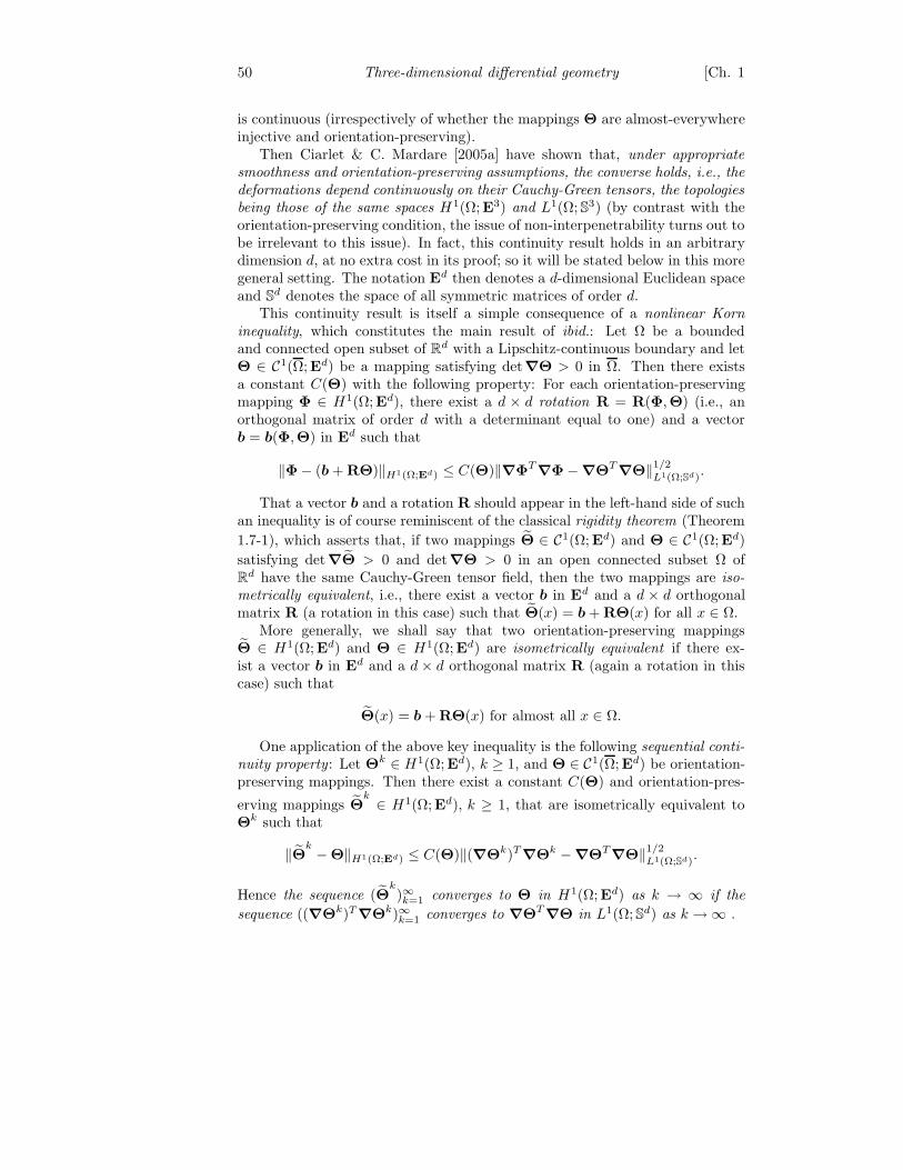
50 Three-dimensional differential geometry [Ch. 1
is continuous (irrespectively of whether the mappings Θ are almost-everywhereinjective and orientation-preserving).
Then Ciarlet & C. Mardare [2005a] have shown that, under appropriate
smoothness and orientation-preserving assumptions, the converse holds, i.e., the
deformations depend continuously on their Cauchy-Green tensors, the topologies
being those of the same spaces H1(Ω;E3) and L1(Ω; S3) (by contrast with theorientation-preserving condition, the issue of non-interpenetrability turns out tobe irrelevant to this issue). In fact, this continuity result holds in an arbitrarydimension d, at no extra cost in its proof; so it will be stated below in this moregeneral setting. The notation Ed then denotes a d-dimensional Euclidean spaceand S
d denotes the space of all symmetric matrices of order d.This continuity result is itself a simple consequence of a nonlinear Korn
inequality, which constitutes the main result of ibid.: Let Ω be a boundedand connected open subset of Rd with a Lipschitz-continuous boundary and letΘ ∈ C1(Ω;Ed) be a mapping satisfying det ∇Θ > 0 in Ω. Then there existsa constant C(Θ) with the following property: For each orientation-preservingmapping Φ ∈ H1(Ω;Ed), there exist a d × d rotation R = R(Φ,Θ) (i.e., anorthogonal matrix of order d with a determinant equal to one) and a vectorb = b(Φ,Θ) in Ed such that
‖Φ− (b+ RΘ)‖H1(Ω;Ed) ≤ C(Θ)‖∇ΦT∇Φ − ∇ΘT
∇Θ‖1/2
L1(Ω;Sd).
That a vector b and a rotation R should appear in the left-hand side of suchan inequality is of course reminiscent of the classical rigidity theorem (Theorem
1.7-1), which asserts that, if two mappings Θ ∈ C1(Ω;Ed) and Θ ∈ C1(Ω;Ed)
satisfying det ∇Θ > 0 and det ∇Θ > 0 in an open connected subset Ω ofRd have the same Cauchy-Green tensor field, then the two mappings are iso-
metrically equivalent, i.e., there exist a vector b in Ed and a d × d orthogonalmatrix R (a rotation in this case) such that Θ(x) = b+ RΘ(x) for all x ∈ Ω.
More generally, we shall say that two orientation-preserving mappingsΘ ∈ H1(Ω;Ed) and Θ ∈ H1(Ω;Ed) are isometrically equivalent if there ex-ist a vector b in Ed and a d × d orthogonal matrix R (again a rotation in thiscase) such that
Θ(x) = b+ RΘ(x) for almost all x ∈ Ω.
One application of the above key inequality is the following sequential conti-
nuity property : Let Θk ∈ H1(Ω;Ed), k ≥ 1, and Θ ∈ C1(Ω;Ed) be orientation-preserving mappings. Then there exist a constant C(Θ) and orientation-pres-
erving mappings Θk ∈ H1(Ω;Ed), k ≥ 1, that are isometrically equivalent to
Θk such that
‖Θk −Θ‖H1(Ω;Ed) ≤ C(Θ)‖(∇Θk)T∇Θk − ∇ΘT
∇Θ‖1/2
L1(Ω;Sd).
Hence the sequence (Θk)∞k=1 converges to Θ in H1(Ω;Ed) as k → ∞ if the
sequence ((∇Θk)T ∇Θk)∞k=1 converges to ∇ΘT∇Θ in L1(Ω; Sd) as k → ∞ .

Sect. 1.8] An immersion as a function of its metric tensor 51
Should the Cauchy-Green strain tensor be viewed as the primary unknown(as suggested above), such a sequential continuity could thus prove to be use-ful when considering infimizing sequences of the total energy, in particular forhandling the part of the energy that takes into account the applied forces andthe boundary conditions, which are both naturally expressed in terms of thedeformation itself.
They key inequality is first established in the special case where Θ is theidentity mapping of the set Ω, by making use in particular of a fundamental“geometric rigidity lemma” recently proved by Friesecke, James & Muller [2002].It is then extended to an arbitrary mapping Θ ∈ C1(Ω; Rn) satisfying det ∇Θ >0 in Ω, thanks in particular to a methodology that bears some similarity withthat used in Theorems 1.8-2 and 1.8-3.
Such results are to be compared with the earlier, pioneering estimates ofJohn [1961], John [1972] and Kohn [1982], which implied continuity at rigid body
deformations, i.e., at a mapping Θ that is isometrically equivalent to the identitymapping of Ω. The recent and noteworthy continuity result of Reshetnyak [2003]for quasi-isometric mappings is in a sense complementary to the above one (italso deals with Sobolev type norms).


Chapter 2
DIFFERENTIAL GEOMETRY OF SURFACES
2.1 CURVILINEAR COORDINATES ON A SURFACE
In addition to the rules governing Latin indices that we set in Section 1.1, wehenceforth require that Greek indices and exponents vary in the set 1, 2 andthat the summation convention be systematically used in conjunction with theserules. For instance, the relation
∂α(ηiai) = (ηβ|α − bαβη3)a
β + (η3|α + bβαηβ)a3
means that, for α = 1, 2,
∂α
( 3∑
i=1
ηiai)
=
2∑
β=1
(ηβ|α − bαβη3)aβ +
(η3|α +
2∑
β=1
bβαηβ
)a3.
Kronecker’s symbols are designated by δβα, δαβ, or δαβ according to the con-
text.
Let there be given as in Section 1.1 a three-dimensional Euclidean space E3,equipped with an orthonormal basis consisting of three vectors ei = ei, and leta · b, |a|, and a ∧ b denote the Euclidean inner product, the Euclidean norm,and the vector product of vectors a, b in the space E3.
In addition, let there be given a two-dimensional vector space, in which twovectors eα = eα form a basis. This space will be identified with R2. Let yα
denote the coordinates of a point y ∈ R2 and let ∂α := ∂/∂yα and ∂αβ :=∂2/∂yα∂yβ.
Finally, let there be given an open subset ω of R2 and a smooth enoughmapping θ : ω → E3 (specific smoothness assumptions on θ will be made later,according to each context). The set
ω := θ(ω)
is called a surface in E3.
53
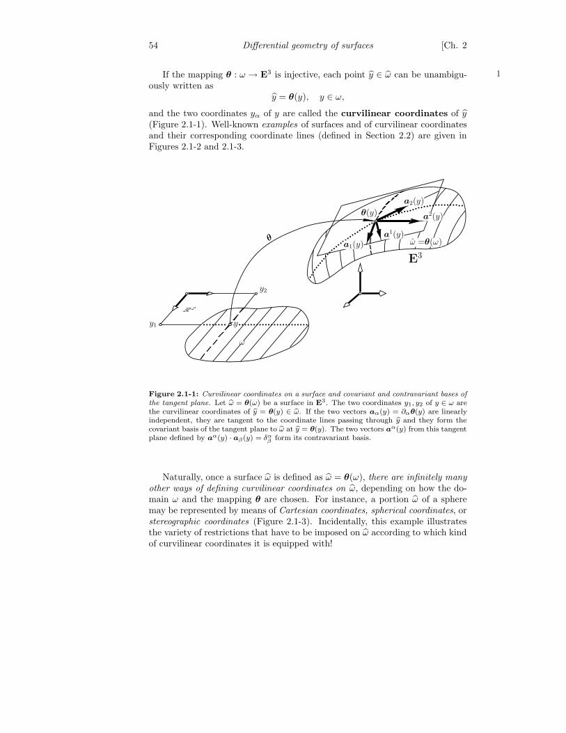
54 Differential geometry of surfaces [Ch. 2
If the mapping θ : ω → E3 is injective, each point y ∈ ω can be unambigu-ously written as
y = θ(y), y ∈ ω,
and the two coordinates yα of y are called the curvilinear coordinates of y(Figure 2.1-1). Well-known examples of surfaces and of curvilinear coordinatesand their corresponding coordinate lines (defined in Section 2.2) are given inFigures 2.1-2 and 2.1-3.
1
y1 y
ω
y2
R 2
θ
θ(y)
a1(y)a
1(y)
a2(y)
ω =θ(ω)
E3
a2(y)
Figure 2.1-1: Curvilinear coordinates on a surface and covariant and contravariant bases of
the tangent plane. Let bω = θ(ω) be a surface in E3. The two coordinates y1, y2 of y ∈ ω arethe curvilinear coordinates of by = θ(y) ∈ bω. If the two vectors aα(y) = ∂αθ(y) are linearlyindependent, they are tangent to the coordinate lines passing through by and they form thecovariant basis of the tangent plane to bω at by = θ(y). The two vectors aα(y) from this tangentplane defined by aα(y) · aβ(y) = δα
β form its contravariant basis.
Naturally, once a surface ω is defined as ω = θ(ω), there are infinitely many
other ways of defining curvilinear coordinates on ω, depending on how the do-main ω and the mapping θ are chosen. For instance, a portion ω of a spheremay be represented by means of Cartesian coordinates, spherical coordinates, orstereographic coordinates (Figure 2.1-3). Incidentally, this example illustratesthe variety of restrictions that have to be imposed on ω according to which kindof curvilinear coordinates it is equipped with!
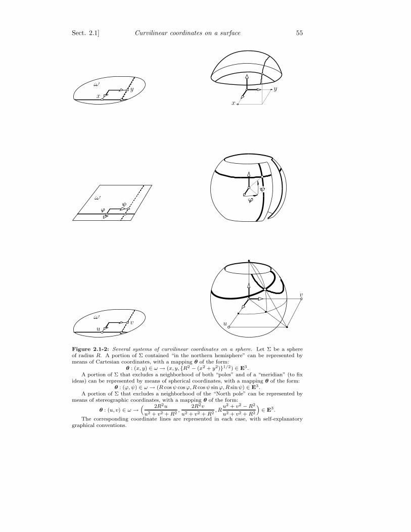
Sect. 2.1] Curvilinear coordinates on a surface 55
1
x
yω
x
y
ψϕ
ω ϕ
ψ
u
vω
u
v
Figure 2.1-2: Several systems of curvilinear coordinates on a sphere. Let Σ be a sphereof radius R. A portion of Σ contained “in the northern hemisphere” can be represented bymeans of Cartesian coordinates, with a mapping θ of the form:
θ : (x, y) ∈ ω → (x, y, R2 − (x2 + y2)1/2) ∈ E3.A portion of Σ that excludes a neighborhood of both “poles” and of a “meridian” (to fix
ideas) can be represented by means of spherical coordinates, with a mapping θ of the form:θ : (ϕ, ψ) ∈ ω → (R cosψ cosϕ,R cosψ sinϕ,R sinψ) ∈ E3.
A portion of Σ that excludes a neighborhood of the “North pole” can be represented bymeans of stereographic coordinates, with a mapping θ of the form:
θ : (u, v) ∈ ω →“ 2R2u
u2 + v2 +R2,
2R2v
u2 + v2 + R2, R
u2 + v2 −R2
u2 + v2 +R2
”∈ E3.
The corresponding coordinate lines are represented in each case, with self-explanatorygraphical conventions.
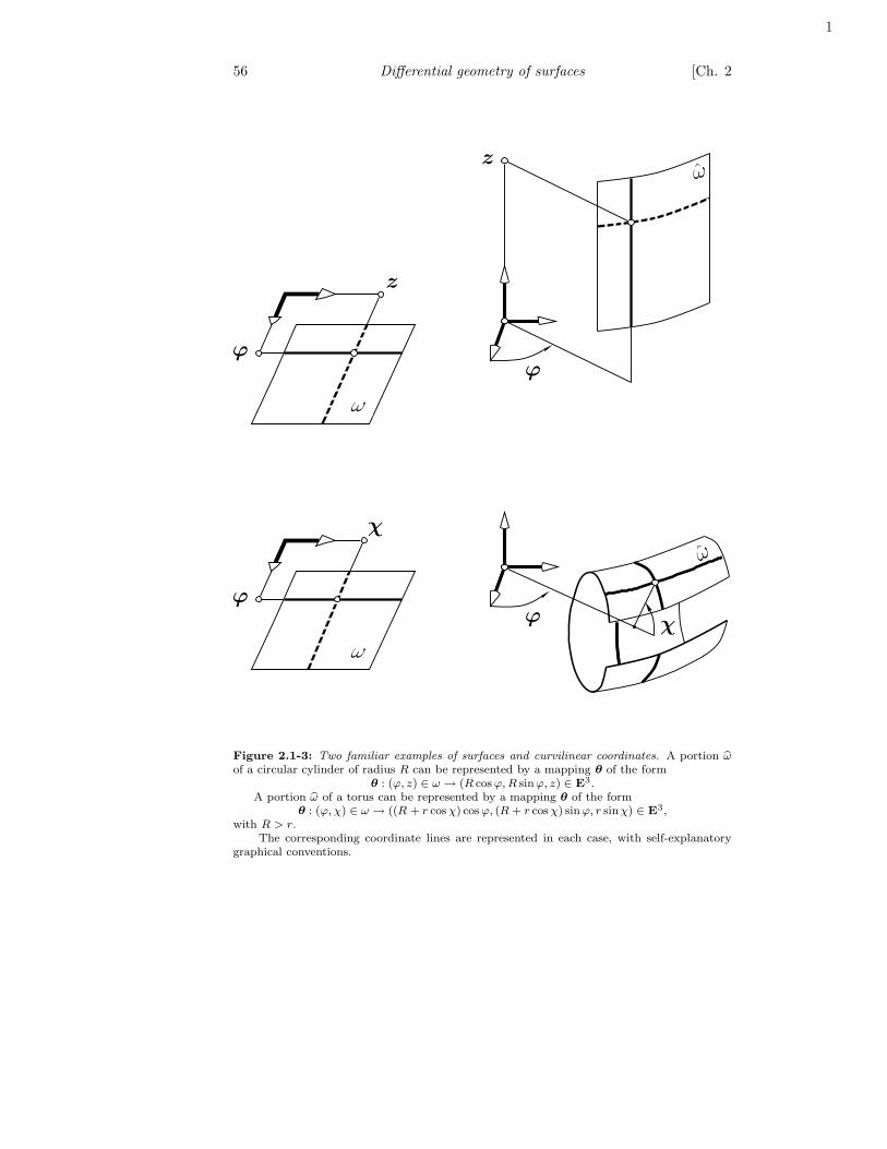
56 Differential geometry of surfaces [Ch. 2
1
ω
ϕ
z
ϕ
zω
ω
ϕ
χ
ϕχ
ω
Figure 2.1-3: Two familiar examples of surfaces and curvilinear coordinates. A portion bωof a circular cylinder of radius R can be represented by a mapping θ of the form
θ : (ϕ, z) ∈ ω → (R cosϕ,R sinϕ, z) ∈ E3.
A portion bω of a torus can be represented by a mapping θ of the formθ : (ϕ, χ) ∈ ω → ((R + r cosχ) cosϕ, (R+ r cosχ) sinϕ, r sinχ) ∈ E3,
with R > r.The corresponding coordinate lines are represented in each case, with self-explanatory
graphical conventions.

Sect. 2.2] First fundamental form 57
2.2 FIRST FUNDAMENTAL FORM
Let ω be an open subset of R2 and let
θ = θiei : ω ⊂ R
2 → θ(ω) = ω ⊂ E3
be a mapping that is differentiable at a point y ∈ ω. If δy is such that (y+δy) ∈ω, then
θ(y + δy) = θ(y) + ∇θ(y)δy + o(δy),
where the 3 × 2 matrix ∇θ(y) is defined by
∇θ(y) :=
∂1θ1 ∂2θ1
∂1θ2 ∂2θ2
∂1θ3 ∂2θ3
(y).
Let the two vectors aα(y) ∈ R3 be defined by
aα(y) := ∂αθ(y) =
∂αθ1
∂αθ2
∂αθ3
(y),
i.e., aα(y) is the α-th column vector of the matrix ∇θ(y) and let δy = δyαeα.Then the expansion of θ about y may be also written as
θ(y + δy) = θ(y) + δyαaα(y) + o(δy).
If in particular δy is of the form δy = δteα, where δt ∈ R and eα is one ofthe basis vectors in R
2, this relation reduces to
θ(y + δteα) = θ(y) + δtaα(y) + o(δt).
A mapping θ : ω → E3 is an immersion at y ∈ ω if it is differentiable aty and the 3 × 2 matrix ∇θ(y) is of rank two, or equivalently if the two vectorsaα(y) = ∂αθ(y) are linearly independent.
Assume from now on in this section that the mapping θ is an immersion
at y. In this case, the last relation shows that each vector aα(y) is tangent
to the α-th coordinate line passing through y = θ(y), defined as the imageby θ of the points of ω that lie on a line parallel to eα passing through y(there exist t0 and t1 with t0 < 0 < t1 such that the α-th coordinate line isgiven by t ∈ ]t0, t1[ → fα(t) := θ(y + teα) in a neighborhood of y; hencef ′
α(0) = ∂αθ(y) = aα(y)); see Figures 2.1-1, 2.1-2, and 2.1-3.The vectors aα(y), which thus span the tangent plane to the surface ω at
y = θ(y), form the covariant basis of the tangent plane to ω at y; seeFigure 2.1-1.
Returning to a general increment δy = δyαeα, we also infer from the expan-sion of θ about y that
|θ(y + δy) − θ(y)|2 = δyT∇θ(y)T
∇θ(y)δy + o(|δy|2)= δyαaα(y) · aβ(y)δyβ + o(|δy|2).
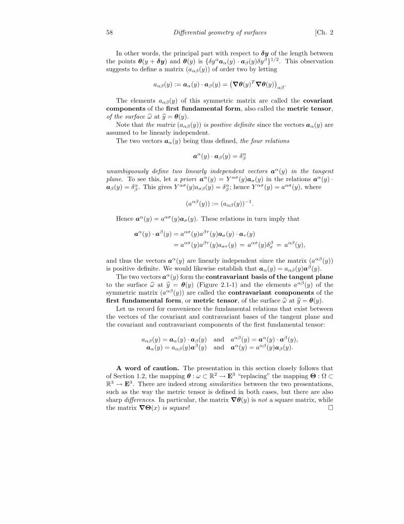
58 Differential geometry of surfaces [Ch. 2
In other words, the principal part with respect to δy of the length betweenthe points θ(y + δy) and θ(y) is δyαaα(y) · aβ(y)δyβ1/2. This observationsuggests to define a matrix (aαβ(y)) of order two by letting
aαβ(y) := aα(y) · aβ(y) =(∇θ(y)T
∇θ(y))αβ
.
The elements aαβ(y) of this symmetric matrix are called the covariant
components of the first fundamental form, also called the metric tensor,of the surface ω at y = θ(y).
Note that the matrix (aαβ(y)) is positive definite since the vectors aα(y) areassumed to be linearly independent.
The two vectors aα(y) being thus defined, the four relations
aα(y) · aβ(y) = δαβ
unambiguously define two linearly independent vectors aα(y) in the tangent
plane. To see this, let a priori aα(y) = Y ασ(y)aσ(y) in the relations aα(y) ·aβ(y) = δα
β . This gives Y ασ(y)aσβ(y) = δαβ ; hence Y ασ(y) = aασ(y), where
(aαβ(y)) := (aαβ(y))−1.
Hence aα(y) = aασ(y)aσ(y). These relations in turn imply that
aα(y) · aβ(y) = aασ(y)aβτ (y)aσ(y) · aτ (y)
= aασ(y)aβτ (y)aστ (y) = aασ(y)δβσ = aαβ(y),
and thus the vectors aα(y) are linearly independent since the matrix (aαβ(y))is positive definite. We would likewise establish that aα(y) = aαβ(y)aβ(y).
The two vectors aα(y) form the contravariant basis of the tangent plane
to the surface ω at y = θ(y) (Figure 2.1-1) and the elements aαβ(y) of thesymmetric matrix (aαβ(y)) are called the contravariant components of thefirst fundamental form, or metric tensor, of the surface ω at y = θ(y).
Let us record for convenience the fundamental relations that exist betweenthe vectors of the covariant and contravariant bases of the tangent plane andthe covariant and contravariant components of the first fundamental tensor:
aαβ(y) = aα(y) · aβ(y) and aαβ(y) = aα(y) · aβ(y),aα(y) = aαβ(y)aβ(y) and aα(y) = aαβ(y)aβ(y).
A word of caution. The presentation in this section closely follows thatof Section 1.2, the mapping θ : ω ⊂ R2 → E3 “replacing” the mapping Θ : Ω ⊂R3 → E3. There are indeed strong similarities between the two presentations,such as the way the metric tensor is defined in both cases, but there are alsosharp differences. In particular, the matrix ∇θ(y) is not a square matrix, whilethe matrix ∇Θ(x) is square!
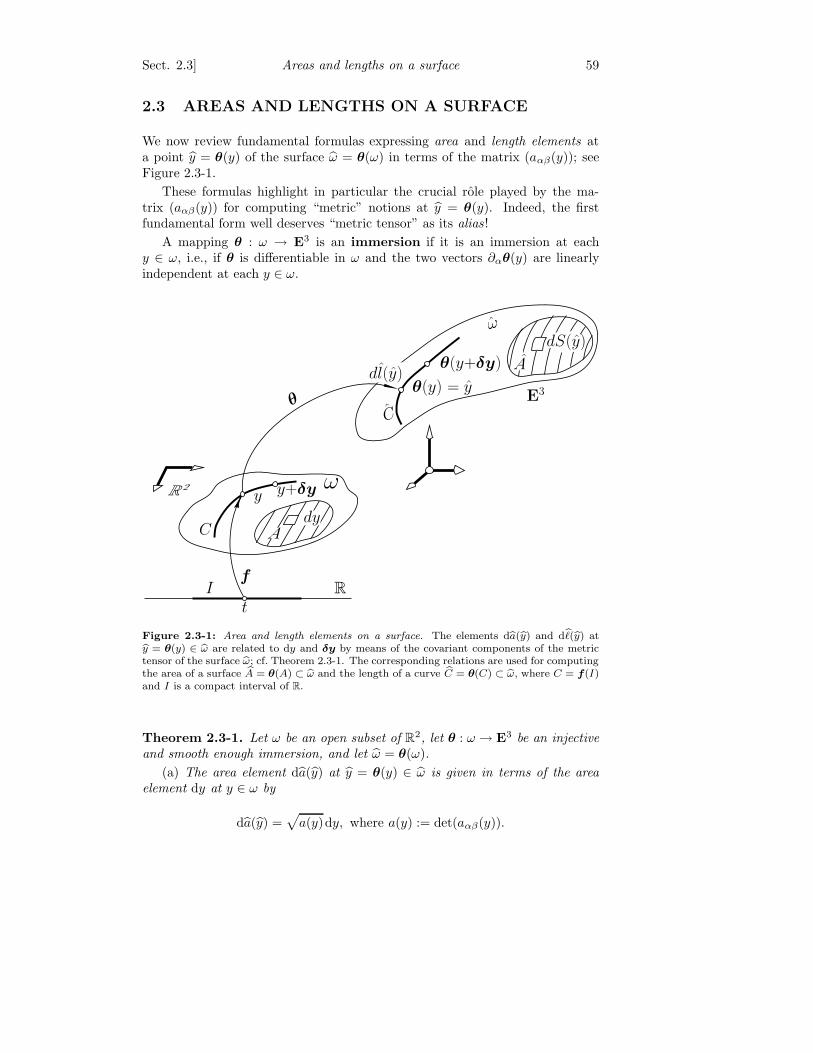
Sect. 2.3] Areas and lengths on a surface 59
2.3 AREAS AND LENGTHS ON A SURFACE
We now review fundamental formulas expressing area and length elements ata point y = θ(y) of the surface ω = θ(ω) in terms of the matrix (aαβ(y)); seeFigure 2.3-1.
These formulas highlight in particular the crucial role played by the ma-trix (aαβ(y)) for computing “metric” notions at y = θ(y). Indeed, the firstfundamental form well deserves “metric tensor” as its alias !
A mapping θ : ω → E3 is an immersion if it is an immersion at eachy ∈ ω, i.e., if θ is differentiable in ω and the two vectors ∂αθ(y) are linearlyindependent at each y ∈ ω.
θ(y+δy)
y+δy
Ady
dl(y)θ(y) = y
C
E3
θ
If
t
R 2
R
ω
y
C
ω
dS(y)
A
Figure 2.3-1: Area and length elements on a surface. The elements dba(by) and db(by) atby = θ(y) ∈ bω are related to dy and δy by means of the covariant components of the metrictensor of the surface bω; cf. Theorem 2.3-1. The corresponding relations are used for computingthe area of a surface bA = θ(A) ⊂ bω and the length of a curve bC = θ(C) ⊂ bω, where C = f(I)and I is a compact interval of R.
Theorem 2.3-1. Let ω be an open subset of R2, let θ : ω → E3 be an injective
and smooth enough immersion, and let ω = θ(ω).
(a) The area element da(y) at y = θ(y) ∈ ω is given in terms of the area
element dy at y ∈ ω by
da(y) =√
a(y)dy, where a(y) := det(aαβ(y)).
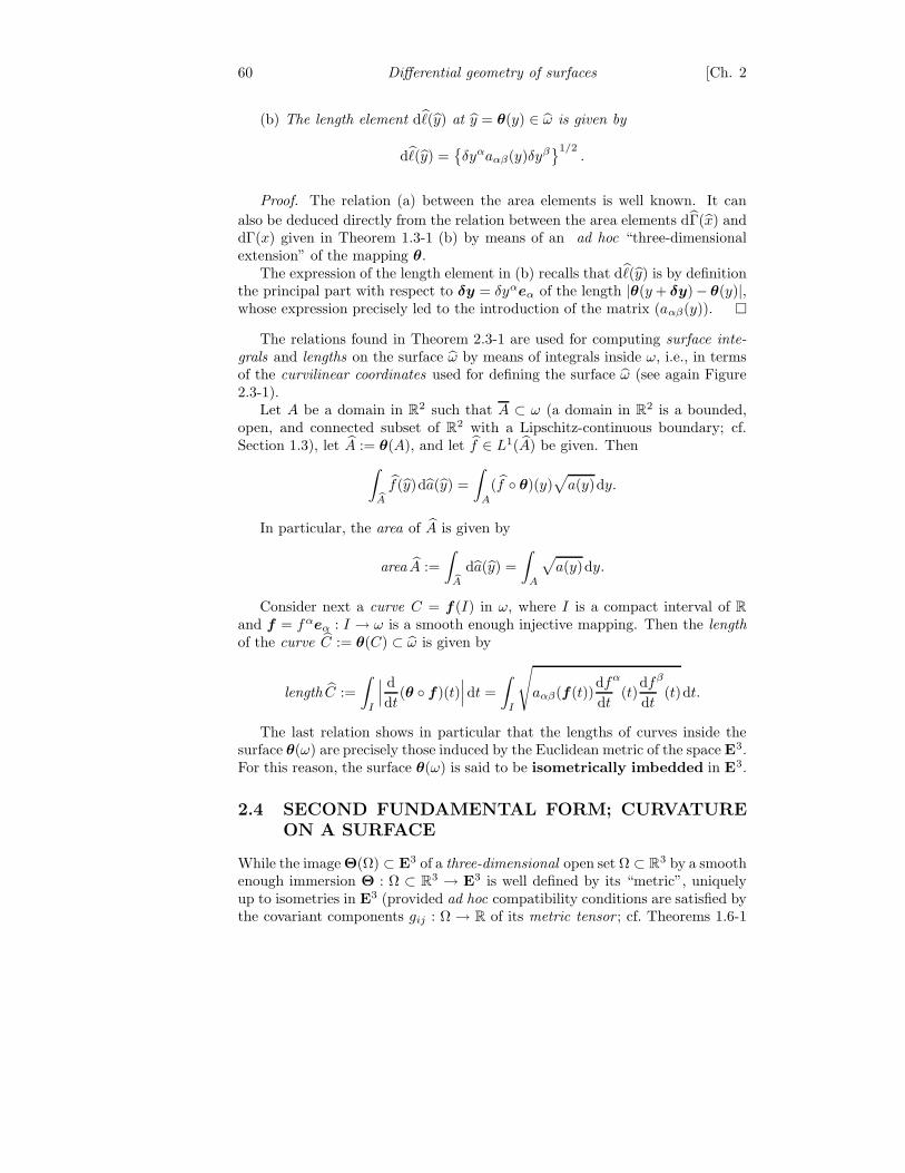
60 Differential geometry of surfaces [Ch. 2
(b) The length element d(y) at y = θ(y) ∈ ω is given by
d(y) =δyαaαβ(y)δyβ
1/2.
Proof. The relation (a) between the area elements is well known. It can
also be deduced directly from the relation between the area elements dΓ(x) anddΓ(x) given in Theorem 1.3-1 (b) by means of an ad hoc “three-dimensionalextension” of the mapping θ.
The expression of the length element in (b) recalls that d(y) is by definitionthe principal part with respect to δy = δyαeα of the length |θ(y + δy)− θ(y)|,whose expression precisely led to the introduction of the matrix (aαβ(y)).
The relations found in Theorem 2.3-1 are used for computing surface inte-
grals and lengths on the surface ω by means of integrals inside ω, i.e., in termsof the curvilinear coordinates used for defining the surface ω (see again Figure2.3-1).
Let A be a domain in R2 such that A ⊂ ω (a domain in R2 is a bounded,open, and connected subset of R2 with a Lipschitz-continuous boundary; cf.Section 1.3), let A := θ(A), and let f ∈ L1(A) be given. Then
∫
bAf(y)da(y) =
∫
A
(f θ)(y)√
a(y)dy.
In particular, the area of A is given by
area A :=
∫
bAda(y) =
∫
A
√a(y)dy.
Consider next a curve C = f (I) in ω, where I is a compact interval of R
and f = fαeα : I → ω is a smooth enough injective mapping. Then the length
of the curve C := θ(C) ⊂ ω is given by
length C :=
∫
I
∣∣∣ d
dt(θ f)(t)
∣∣∣dt =
∫
I
√
aαβ(f(t))df
dt
α
(t)df
dt
β
(t)dt.
The last relation shows in particular that the lengths of curves inside thesurface θ(ω) are precisely those induced by the Euclidean metric of the space E3.For this reason, the surface θ(ω) is said to be isometrically imbedded in E3.
2.4 SECOND FUNDAMENTAL FORM; CURVATURE
ON A SURFACE
While the image Θ(Ω) ⊂ E3 of a three-dimensional open set Ω ⊂ R3 by a smooth
enough immersion Θ : Ω ⊂ R3 → E3 is well defined by its “metric”, uniquelyup to isometries in E3 (provided ad hoc compatibility conditions are satisfied bythe covariant components gij : Ω → R of its metric tensor ; cf. Theorems 1.6-1
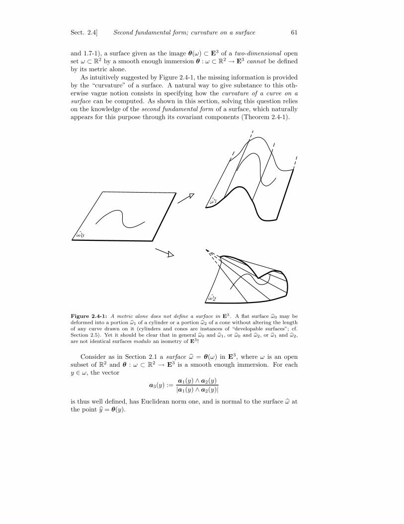
Sect. 2.4] Second fundamental form; curvature on a surface 61
and 1.7-1), a surface given as the image θ(ω) ⊂ E3 of a two-dimensional openset ω ⊂ R2 by a smooth enough immersion θ : ω ⊂ R2 → E3 cannot be definedby its metric alone.
As intuitively suggested by Figure 2.4-1, the missing information is providedby the “curvature” of a surface. A natural way to give substance to this oth-erwise vague notion consists in specifying how the curvature of a curve on a
surface can be computed. As shown in this section, solving this question relieson the knowledge of the second fundamental form of a surface, which naturallyappears for this purpose through its covariant components (Theorem 2.4-1).
ω0
ω1
ω2
Figure 2.4-1: A metric alone does not define a surface in E3. A flat surface bω0 may bedeformed into a portion bω1 of a cylinder or a portion bω2 of a cone without altering the lengthof any curve drawn on it (cylinders and cones are instances of “developable surfaces”; cf.Section 2.5). Yet it should be clear that in general bω0 and bω1, or bω0 and bω2, or bω1 and bω2,are not identical surfaces modulo an isometry of E3!
Consider as in Section 2.1 a surface ω = θ(ω) in E3, where ω is an opensubset of R2 and θ : ω ⊂ R2 → E3 is a smooth enough immersion. For eachy ∈ ω, the vector
a3(y) :=a1(y) ∧ a2(y)
|a1(y) ∧ a2(y)|is thus well defined, has Euclidean norm one, and is normal to the surface ω atthe point y = θ(y).
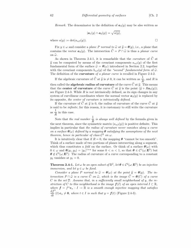
62 Differential geometry of surfaces [Ch. 2
Remark. The denominator in the definition of a3(y) may be also written as
|a1(y) ∧ a2(y)| =√
a(y),
where a(y) := det(aαβ(y)).
Fix y ∈ ω and consider a plane P normal to ω at y = θ(y), i.e., a plane that
contains the vector a3(y). The intersection C = P ∩ ω is thus a planar curve
on ω.
As shown in Theorem 2.4-1, it is remarkable that the curvature of C aty can be computed by means of the covariant components aαβ(y) of the firstfundamental form of the surface ω = θ(ω) introduced in Section 2.2, togetherwith the covariant components bαβ(y) of the “second” fundamental form of ω.The definition of the curvature of a planar curve is recalled in Figure 2.4-2.
If the algebraic curvature of C at y is 6= 0, it can be written as1
R, and R is
then called the algebraic radius of curvature of the curve C at y. This meansthat the center of curvature of the curve C at y is the point (y + Ra3(y));see Figure 2.4-3. While R is not intrinsically defined, as its sign changes in anysystem of curvilinear coordinates where the normal vector a3(y) is replaced byits opposite, the center of curvature is intrinsically defined.
If the curvature of C at y is 0, the radius of curvature of the curve C at yis said to be infinite; for this reason, it is customary to still write the curvature
as1
Rin this case.
Note that the real number1
Ris always well defined by the formula given in
the next theorem, since the symmetric matrix (aαβ(y)) is positive definite. Thisimplies in particular that the radius of curvature never vanishes along a curve
on a surface θ(ω) defined by a mapping θ satisfying the assumptions of the next
theorem, hence in particular of class C2 on ω.
It is intuitively clear that if R = 0, the mapping θ “cannot be too smooth”.Think of a surface made of two portions of planes intersecting along a segment,which thus constitutes a fold on the surface. Or think of a surface θ(ω) with0 ∈ ω and θ(y1, y2) = |y1|1+α for some 0 < α < 1, so that θ ∈ C1(ω;E3) butθ /∈ C2(ω;E3): The radius of curvature of a curve corresponding to a constanty2 vanishes at y1 = 0.
Theorem 2.4-1. Let ω be an open subset of R2, let θ ∈ C2(ω;E3) be an injective
immersion, and let y ∈ ω be fixed.
Consider a plane P normal to ω = θ(ω) at the point y = θ(y). The in-
tersection P ∩ ω is a curve C on ω, which is the image C = θ(C) of a curve
C in the set ω. Assume that, in a sufficiently small neighborhood of y, the re-
striction of C to this neighborhood is the image f(I) of an open interval I ⊂ R,
where f = fαeα : I → R is a smooth enough injective mapping that satisfiesdf
dt
α
(t) eα 6= 0, where t ∈ I is such that y = f(t) (Figure 2.4-3).
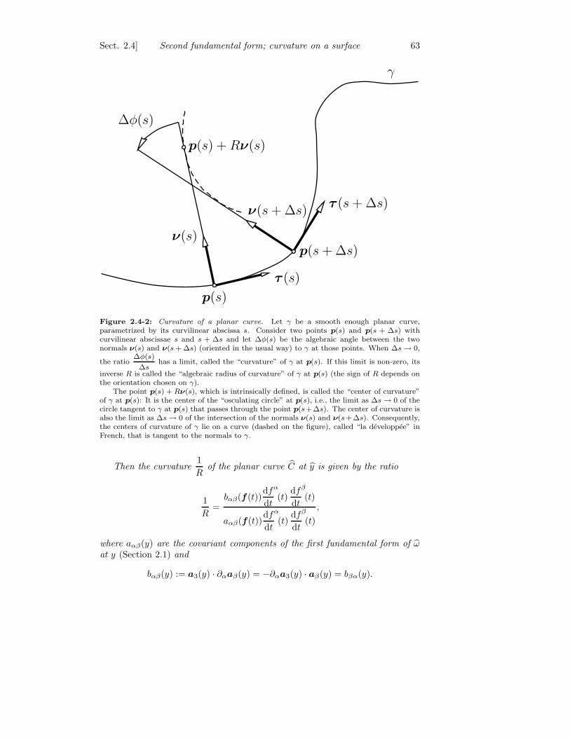
Sect. 2.4] Second fundamental form; curvature on a surface 63
∆φ(s)
p(s) + Rν(s)
γ
ν(s)
ν(s + ∆s)
p(s)
p(s + ∆s)
τ (s + ∆s)
τ (s)
Figure 2.4-2: Curvature of a planar curve. Let γ be a smooth enough planar curve,parametrized by its curvilinear abscissa s. Consider two points p(s) and p(s + ∆s) withcurvilinear abscissae s and s + ∆s and let ∆φ(s) be the algebraic angle between the twonormals ν(s) and ν(s+ ∆s) (oriented in the usual way) to γ at those points. When ∆s→ 0,
the ratio∆φ(s)
∆shas a limit, called the “curvature” of γ at p(s). If this limit is non-zero, its
inverse R is called the “algebraic radius of curvature” of γ at p(s) (the sign of R depends onthe orientation chosen on γ).
The point p(s) + Rν(s), which is intrinsically defined, is called the “center of curvature”of γ at p(s): It is the center of the “osculating circle” at p(s), i.e., the limit as ∆s→ 0 of thecircle tangent to γ at p(s) that passes through the point p(s+∆s). The center of curvature isalso the limit as ∆s→ 0 of the intersection of the normals ν(s) and ν(s+∆s). Consequently,the centers of curvature of γ lie on a curve (dashed on the figure), called “la developpee” inFrench, that is tangent to the normals to γ.
Then the curvature1
Rof the planar curve C at y is given by the ratio
1
R=
bαβ(f (t))df
dt
α
(t)df
dt
β
(t)
aαβ(f(t))df
dt
α
(t)df
dt
β
(t)
,
where aαβ(y) are the covariant components of the first fundamental form of ωat y (Section 2.1) and
bαβ(y) := a3(y) · ∂αaβ(y) = −∂αa3(y) · aβ(y) = bβα(y).
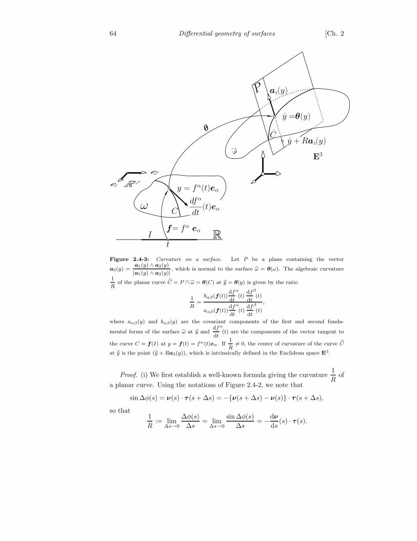
64 Differential geometry of surfaces [Ch. 2
y =θ(y)
C
P
y + Ra3(y)
a3(y)
E3
θ
If= fα eα
t
e2
e1 R 2
R
dfα
dt(t)eα
ω
y = fα(t)eα
Cω
Figure 2.4-3: Curvature on a surface. Let P be a plane containing the vector
a3(y) =a1(y) ∧ a2(y)
|a1(y) ∧ a2(y)|, which is normal to the surface bω = θ(ω). The algebraic curvature
1
Rof the planar curve bC = P ∩ bω = θ(C) at by = θ(y) is given by the ratio
1
R=bαβ(f(t))
df
dt
α
(t)df
dt
β
(t)
aαβ(f(t))df
dt
α
(t)df
dt
β
(t)
,
where aαβ(y) and bαβ(y) are the covariant components of the first and second funda-
mental forms of the surface bω at by anddf
dt
α
(t) are the components of the vector tangent to
the curve C = f(I) at y = f(t) = fα(t)eα. If1
R6= 0, the center of curvature of the curve bC
at by is the point (by + Ra3(y)), which is intrinsically defined in the Euclidean space E3.
Proof. (i) We first establish a well-known formula giving the curvature1
Rof
a planar curve. Using the notations of Figure 2.4-2, we note that
sin ∆φ(s) = ν(s) · τ (s + ∆s) = −ν(s + ∆s) − ν(s) · τ (s + ∆s),
so that1
R:= lim
∆s→0
∆φ(s)
∆s= lim
∆s→0
sin ∆φ(s)
∆s= −dν
ds(s) · τ (s).
Sect. 2.5] Second fundamental form; curvature on a surface 65
(ii) The curve (θ f)(I), which is a priori parametrized by t ∈ I , can bealso parametrized by its curvilinear abscissa s in a neighborhood of the point y.There thus exist an interval I ⊂ I and a mapping p : J → P , where J ⊂ R isan interval, such that
(θ f)(t) = p(s) and (a3 f)(t) = ν(s) for all t ∈ I , s ∈ J.
By (i), the curvature1
Rof C is given by
1
R= −dν
ds(s) · τ (s),
where
dν
ds(s) =
d(a3 f)
dt(t)
dt
ds= ∂αa3(f(t))
df
dt
α
(t)dt
ds,
τ (s) =dp
ds(s) =
d(θ f )
dt(t)
dt
ds
= ∂βθ(f (t))df
dt
β
(t)dt
ds= aβ(f(t))
df
dt
β
(t)dt
ds.
Hence1
R= −∂αa3(f (t)) · aβ(f(t))
df
dt
α
(t)df
dt
β
(t)
(dt
ds
)2
.
To obtain the announced expression for1
R, it suffices to note that
−∂αa3(f (t)) · aβ(f(t)) = bαβ(f(t)),
by definition of the functions bαβ and that (Theorem 2.3-1 (b))
ds =δyαaαβ(y)δyβ
1/2=
aαβ(f (t))
df
dt
α
(t)df
dt
β
(t)1/2
dt.
The knowledge of the curvatures of curves contained in planes normal to ωsuffices for computing the curvature of any curve on ω. More specifically, theradius of curvature R at y of any smooth enough curve C (planar or not) on the
surface ω is given bycosϕ
R=
1
R, where ϕ is the angle between the “principal
normal” to C at y and a3(y) and1
Ris given in Theorem 2.4-1; see, e.g., Stoker
[1969, Chapter 4, Section 12].The elements bαβ(y) of the symmetric matrix (bαβ(y)) defined in Theorem
2.4-1 are called the covariant components of the second fundamental form
of the surface ω = θ(ω) at y = θ(y).
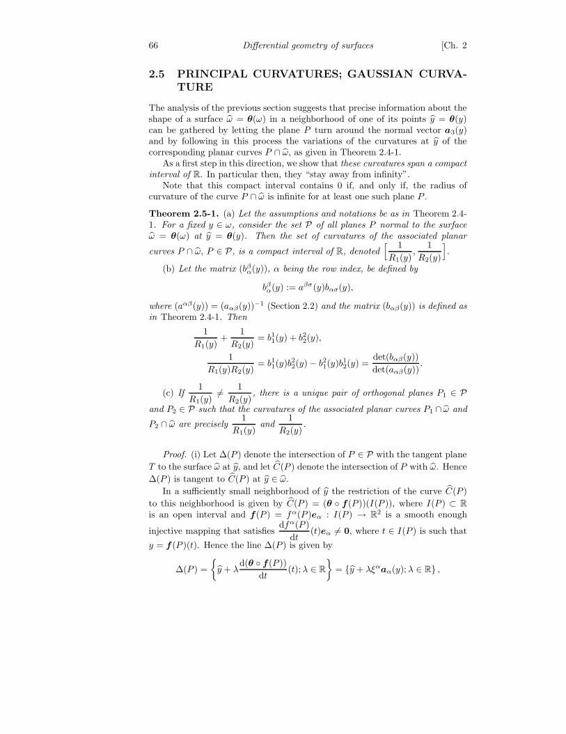
66 Differential geometry of surfaces [Ch. 2
2.5 PRINCIPAL CURVATURES; GAUSSIAN CURVA-
TURE
The analysis of the previous section suggests that precise information about theshape of a surface ω = θ(ω) in a neighborhood of one of its points y = θ(y)can be gathered by letting the plane P turn around the normal vector a3(y)and by following in this process the variations of the curvatures at y of thecorresponding planar curves P ∩ ω, as given in Theorem 2.4-1.
As a first step in this direction, we show that these curvatures span a compact
interval of R. In particular then, they “stay away from infinity”.Note that this compact interval contains 0 if, and only if, the radius of
curvature of the curve P ∩ ω is infinite for at least one such plane P .
Theorem 2.5-1. (a) Let the assumptions and notations be as in Theorem 2.4-1. For a fixed y ∈ ω, consider the set P of all planes P normal to the surface
ω = θ(ω) at y = θ(y). Then the set of curvatures of the associated planar
curves P ∩ ω, P ∈ P, is a compact interval of R, denoted[ 1
R1(y),
1
R2(y)
].
(b) Let the matrix (bβα(y)), α being the row index, be defined by
bβα(y) := aβσ(y)bασ(y),
where (aαβ(y)) = (aαβ(y))−1 (Section 2.2) and the matrix (bαβ(y)) is defined as
in Theorem 2.4-1. Then
1
R1(y)+
1
R2(y)= b1
1(y) + b22(y),
1
R1(y)R2(y)= b1
1(y)b22(y) − b2
1(y)b12(y) =
det(bαβ(y))
det(aαβ(y)).
(c) If1
R1(y)6= 1
R2(y), there is a unique pair of orthogonal planes P1 ∈ P
and P2 ∈ P such that the curvatures of the associated planar curves P1 ∩ ω and
P2 ∩ ω are precisely1
R1(y)and
1
R2(y).
Proof. (i) Let ∆(P ) denote the intersection of P ∈ P with the tangent plane
T to the surface ω at y, and let C(P ) denote the intersection of P with ω. Hence
∆(P ) is tangent to C(P ) at y ∈ ω.
In a sufficiently small neighborhood of y the restriction of the curve C(P )
to this neighborhood is given by C(P ) = (θ f(P ))(I(P )), where I(P ) ⊂ R
is an open interval and f(P ) = fα(P )eα : I(P ) → R2 is a smooth enough
injective mapping that satisfiesdfα(P )
dt(t)eα 6= 0, where t ∈ I(P ) is such that
y = f (P )(t). Hence the line ∆(P ) is given by
∆(P ) =
y + λ
d(θ f(P ))
dt(t); λ ∈ R
= y + λξαaα(y); λ ∈ R ,
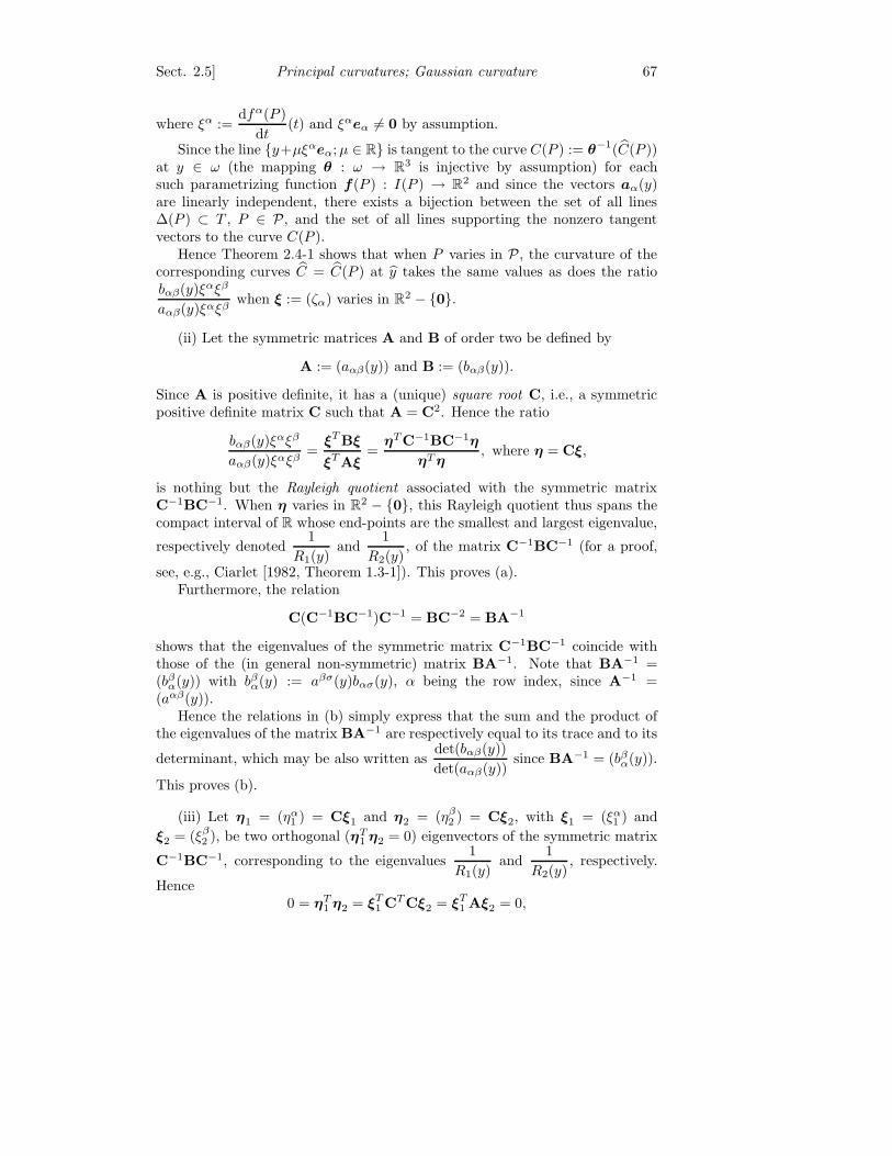
Sect. 2.5] Principal curvatures; Gaussian curvature 67
where ξα :=dfα(P )
dt(t) and ξαeα 6= 0 by assumption.
Since the line y+µξαeα; µ ∈ R is tangent to the curve C(P ) := θ−1(C(P ))at y ∈ ω (the mapping θ : ω → R
3 is injective by assumption) for eachsuch parametrizing function f(P ) : I(P ) → R2 and since the vectors aα(y)are linearly independent, there exists a bijection between the set of all lines∆(P ) ⊂ T , P ∈ P , and the set of all lines supporting the nonzero tangentvectors to the curve C(P ).
Hence Theorem 2.4-1 shows that when P varies in P , the curvature of thecorresponding curves C = C(P ) at y takes the same values as does the ratiobαβ(y)ξαξβ
aαβ(y)ξαξβwhen ξ := (ζα) varies in R2 − 0.
(ii) Let the symmetric matrices A and B of order two be defined by
A := (aαβ(y)) and B := (bαβ(y)).
Since A is positive definite, it has a (unique) square root C, i.e., a symmetricpositive definite matrix C such that A = C2. Hence the ratio
bαβ(y)ξαξβ
aαβ(y)ξαξβ=ξT Bξ
ξT Aξ=ηT C−1BC−1η
ηTη, where η = Cξ,
is nothing but the Rayleigh quotient associated with the symmetric matrixC−1BC−1. When η varies in R2 − 0, this Rayleigh quotient thus spans thecompact interval of R whose end-points are the smallest and largest eigenvalue,
respectively denoted1
R1(y)and
1
R2(y), of the matrix C−1BC−1 (for a proof,
see, e.g., Ciarlet [1982, Theorem 1.3-1]). This proves (a).Furthermore, the relation
C(C−1BC−1)C−1 = BC−2 = BA−1
shows that the eigenvalues of the symmetric matrix C−1BC−1 coincide withthose of the (in general non-symmetric) matrix BA−1. Note that BA−1 =(bβ
α(y)) with bβα(y) := aβσ(y)bασ(y), α being the row index, since A−1 =
(aαβ(y)).Hence the relations in (b) simply express that the sum and the product of
the eigenvalues of the matrix BA−1 are respectively equal to its trace and to its
determinant, which may be also written asdet(bαβ(y))
det(aαβ(y))since BA−1 = (bβ
α(y)).
This proves (b).
(iii) Let η1 = (ηα1 ) = Cξ1 and η2 = (ηβ
2 ) = Cξ2, with ξ1 = (ξα1 ) and
ξ2 = (ξβ2 ), be two orthogonal (ηT
1 η2 = 0) eigenvectors of the symmetric matrix
C−1BC−1, corresponding to the eigenvalues1
R1(y)and
1
R2(y), respectively.
Hence0 = ηT
1 η2 = ξT1 CT Cξ2 = ξT
1 Aξ2 = 0,

68 Differential geometry of surfaces [Ch. 2
since CT = C. By (i), the corresponding lines ∆(P1) and ∆(P2) of the tangent
plane are parallel to the vectors ξα1 aα(y) and ξβ
2 aβ(y), which are orthogonalsince
ξα1 aα(y)
·ξβ2 aβ(y)
= aαβ(y)ξα
1 ξβ2 = ξT
1 Aξ2.
If1
R1(y)6= 1
R2(y), the directions of the vectors η1 and η2 are uniquely
determined and the lines ∆(P1) and ∆(P2) are likewise uniquely determined.This proves (c).
We are now in a position to state several fundamental definitions :The elements bβ
α(y) of the (in general non-symmetric) matrix (bβα(y)) defined
in Theorem 2.5-1 are called the mixed components of the second funda-
mental form of the surface ω = θ(ω) at y = θ(y).
The real numbers1
R1(y)and
1
R2(y)(one or both possibly equal to 0) found
in Theorem 2.5-1 are called the principal curvatures of ω at y.
If1
R1(y)=
1
R2(y), the curvatures of the planar curves P ∩ ω are the same in
all directions, i.e., for all P ∈ P . If1
R1(y)=
1
R2(y)= 0, the point y = θ(y) is
called a planar point. If1
R1(y)=
1
R2(y)6= 0, y is called an umbilical point.
It is remarkable that, if all the points of ω are planar, then ω is a portion
of a plane. Likewise, if all the points of ω are umbilical, then ω is a portion of
a sphere. For proofs, see, e.g., Stoker [1969, p. 87 and p. 99].Let y = θ(y) ∈ ω be a point that is neither planar nor umbilical; in other
words, the principal curvatures at y are not equal. Then the two orthogonallines tangent to the planar curves P1 ∩ ω and P2 ∩ ω (Theorem 2.5-1 (c)) arecalled the principal directions at y.
A line of curvature is a curve on ω that is tangent to a principal directionat each one of its points. It can be shown that a point that is neither planar
nor umbilical possesses a neighborhood where two orthogonal families of lines
of curvature can be chosen as coordinate lines. See, e.g., Klingenberg [1973,Lemma 3.6.6].
If1
R1(y)6= 0 and
1
R2(y)6= 0, the real numbers R1(y) and R2(y) are called
the algebraic principal radii of curvature of ω at y. If, e.g.,1
R1(y)= 0,
the corresponding radius of curvature R1(y) is said to be infinite, accordingto the convention made in Section 2.4. While the algebraic principal radii ofcurvature may simultaneously change their signs in another system of curvilinearcoordinates, the associated centers of curvature are intrinsically defined.
The numbers( 1
R1(y)+
1
R2(y)
)and
1
R1(y)R2(y), which are the principal
invariants of the matrix (bβα(y)) (Theorem 2.5-1), are respectively called the
mean curvature and the Gaussian, or total, curvature of the surface ωat y.
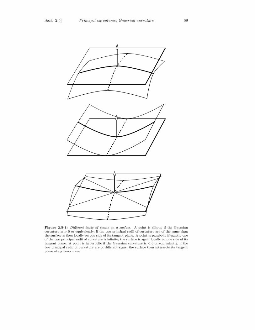
Sect. 2.5] Principal curvatures; Gaussian curvature 69
Figure 2.5-1: Different kinds of points on a surface. A point is elliptic if the Gaussiancurvature is > 0 or equivalently, if the two principal radii of curvature are of the same sign;the surface is then locally on one side of its tangent plane. A point is parabolic if exactly oneof the two principal radii of curvature is infinite; the surface is again locally on one side of itstangent plane. A point is hyperbolic if the Gaussian curvature is < 0 or equivalently, if thetwo principal radii of curvature are of different signs; the surface then intersects its tangentplane along two curves.
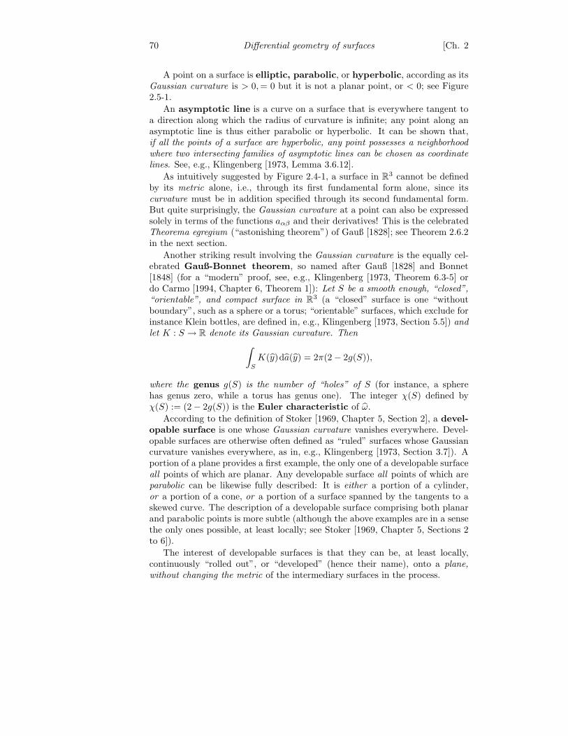
70 Differential geometry of surfaces [Ch. 2
A point on a surface is elliptic, parabolic, or hyperbolic, according as itsGaussian curvature is > 0, = 0 but it is not a planar point, or < 0; see Figure2.5-1.
An asymptotic line is a curve on a surface that is everywhere tangent toa direction along which the radius of curvature is infinite; any point along anasymptotic line is thus either parabolic or hyperbolic. It can be shown that,if all the points of a surface are hyperbolic, any point possesses a neighborhood
where two intersecting families of asymptotic lines can be chosen as coordinate
lines. See, e.g., Klingenberg [1973, Lemma 3.6.12].
As intuitively suggested by Figure 2.4-1, a surface in R3 cannot be definedby its metric alone, i.e., through its first fundamental form alone, since itscurvature must be in addition specified through its second fundamental form.But quite surprisingly, the Gaussian curvature at a point can also be expressedsolely in terms of the functions aαβ and their derivatives! This is the celebratedTheorema egregium (“astonishing theorem”) of Gauß [1828]; see Theorem 2.6.2in the next section.
Another striking result involving the Gaussian curvature is the equally cel-ebrated Gauß-Bonnet theorem, so named after Gauß [1828] and Bonnet[1848] (for a “modern” proof, see, e.g., Klingenberg [1973, Theorem 6.3-5] ordo Carmo [1994, Chapter 6, Theorem 1]): Let S be a smooth enough, “closed”,
“orientable”, and compact surface in R3 (a “closed” surface is one “withoutboundary”, such as a sphere or a torus; “orientable” surfaces, which exclude forinstance Klein bottles, are defined in, e.g., Klingenberg [1973, Section 5.5]) and
let K : S → R denote its Gaussian curvature. Then
∫
S
K(y)da(y) = 2π(2 − 2g(S)),
where the genus g(S) is the number of “holes” of S (for instance, a spherehas genus zero, while a torus has genus one). The integer χ(S) defined byχ(S) := (2 − 2g(S)) is the Euler characteristic of ω.
According to the definition of Stoker [1969, Chapter 5, Section 2], a devel-
opable surface is one whose Gaussian curvature vanishes everywhere. Devel-opable surfaces are otherwise often defined as “ruled” surfaces whose Gaussiancurvature vanishes everywhere, as in, e.g., Klingenberg [1973, Section 3.7]). Aportion of a plane provides a first example, the only one of a developable surfaceall points of which are planar. Any developable surface all points of which areparabolic can be likewise fully described: It is either a portion of a cylinder,or a portion of a cone, or a portion of a surface spanned by the tangents to askewed curve. The description of a developable surface comprising both planarand parabolic points is more subtle (although the above examples are in a sensethe only ones possible, at least locally; see Stoker [1969, Chapter 5, Sections 2to 6]).
The interest of developable surfaces is that they can be, at least locally,continuously “rolled out”, or “developed” (hence their name), onto a plane,
without changing the metric of the intermediary surfaces in the process.
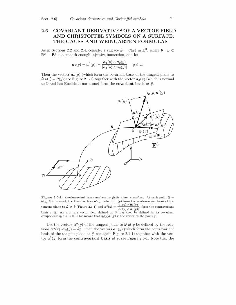
Sect. 2.6] Covariant derivatives and Christoffel symbols 71
2.6 COVARIANT DERIVATIVES OF A VECTOR FIELD
AND CHRISTOFFEL SYMBOLS ON A SURFACE;
THE GAUSS AND WEINGARTEN FORMULAS
As in Sections 2.2 and 2.4, consider a surface ω = θ(ω) in E3, where θ : ω ⊂R2 → E3 is a smooth enough injective immersion, and let
a3(y) = a3(y) :=a1(y) ∧ a2(y)
|a1(y) ∧ a2(y)| , y ∈ ω.
Then the vectors aα(y) (which form the covariant basis of the tangent plane toω at y = θ(y); see Figure 2.1-1) together with the vector a3(y) (which is normalto ω and has Euclidean norm one) form the covariant basis at y.
y
y2
ω
y1
R 2
θy
η3(y)
ηi(y)ai(y)
a3(y)
a2(y)
η2(y) a1(y)
η1(y)
ω =θ(ω)
E3
Figure 2.6-1: Contravariant bases and vector fields along a surface. At each point by =θ(y) ∈ bω = θ(ω), the three vectors ai(y), where aα(y) form the contravariant basis of the
tangent plane to bω at by (Figure 2.1-1) and a3(y) =a1(y) ∧ a2(y)
|a1(y) ∧ a2(y)|, form the contravariant
basis at by. An arbitrary vector field defined on bω may then be defined by its covariantcomponents ηi : ω → R. This means that ηi(y)ai(y) is the vector at the point by.
Let the vectors aα(y) of the tangent plane to ω at y be defined by the rela-tions aα(y) ·aβ(y) = δα
β . Then the vectors aα(y) (which form the contravariantbasis of the tangent plane at y; see again Figure 2.1-1) together with the vec-tor a3(y) form the contravariant basis at y; see Figure 2.6-1. Note that the
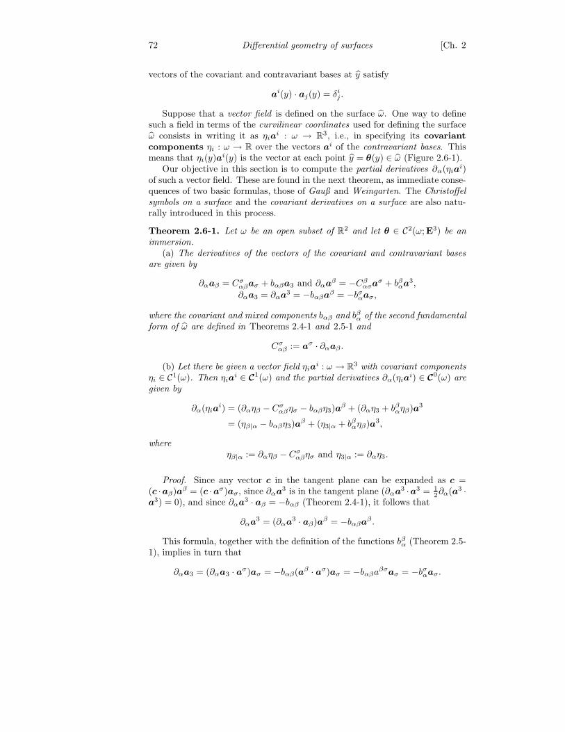
72 Differential geometry of surfaces [Ch. 2
vectors of the covariant and contravariant bases at y satisfy
ai(y) · aj(y) = δij .
Suppose that a vector field is defined on the surface ω. One way to definesuch a field in terms of the curvilinear coordinates used for defining the surfaceω consists in writing it as ηia
i : ω → R3, i.e., in specifying its covariant
components ηi : ω → R over the vectors ai of the contravariant bases. Thismeans that ηi(y)ai(y) is the vector at each point y = θ(y) ∈ ω (Figure 2.6-1).
Our objective in this section is to compute the partial derivatives ∂α(ηiai)
of such a vector field. These are found in the next theorem, as immediate conse-quences of two basic formulas, those of Gauß and Weingarten. The Christoffel
symbols on a surface and the covariant derivatives on a surface are also natu-rally introduced in this process.
Theorem 2.6-1. Let ω be an open subset of R2 and let θ ∈ C2(ω;E3) be an
immersion.
(a) The derivatives of the vectors of the covariant and contravariant bases
are given by
∂αaβ = Cσαβaσ + bαβa3 and ∂αa
β = −Cβασa
σ + bβαa
3,
∂αa3 = ∂αa3 = −bαβa
β = −bσαaσ ,
where the covariant and mixed components bαβ and bβα of the second fundamental
form of ω are defined in Theorems 2.4-1 and 2.5-1 and
Cσαβ := aσ · ∂αaβ .
(b) Let there be given a vector field ηiai : ω → R3 with covariant components
ηi ∈ C1(ω). Then ηiai ∈ C
1(ω) and the partial derivatives ∂α(ηiai) ∈ C
0(ω) are
given by
∂α(ηiai) = (∂αηβ − Cσ
αβησ − bαβη3)aβ + (∂αη3 + bβ
αηβ)a3
= (ηβ|α − bαβη3)aβ + (η3|α + bβ
αηβ)a3,
where
ηβ|α := ∂αηβ − Cσαβησ and η3|α := ∂αη3.
Proof. Since any vector c in the tangent plane can be expanded as c =(c ·aβ)aβ = (c ·aσ)aσ, since ∂αa
3 is in the tangent plane (∂αa3 ·a3 = 1
2∂α(a3 ·a3) = 0), and since ∂αa
3 · aβ = −bαβ (Theorem 2.4-1), it follows that
∂αa3 = (∂αa
3 · aβ)aβ = −bαβaβ .
This formula, together with the definition of the functions bβα (Theorem 2.5-
1), implies in turn that
∂αa3 = (∂αa3 · aσ)aσ = −bαβ(aβ · aσ)aσ = −bαβaβσaσ = −bσαaσ .

Sect. 2.6] Covariant derivatives and Christoffel symbols 73
Any vector c can be expanded as c = (c · ai)ai = (c · aj)aj . In particular,
∂αaβ = (∂αaβ · aσ)aσ + (∂αaβ · a3)a3 = Cσαβaσ + bαβa3,
by definition of Cσαβ and bαβ. Finally,
∂αaβ = (∂αa
β · aσ)aσ + (∂αaβ · a3)a
3 = −Cβασa
σ + bβαa
3,
since∂αa
β · a3 = −aβ · ∂αa3 = bσαaσ · aβ = bβ
α.
That ηiai ∈ C
1(ω) if ηi ∈ C1(ω) is clear since ai ∈ C1(ω) if θ ∈ C2(ω;E3).The formulas established supra immediately lead to the announced expressionof ∂α(ηia
i).
The relations (found in Theorem 2.6-1)
∂αaβ = Cσαβaσ + bαβa3 and ∂αa
β = −Cβασa
σ + bβαa
3
and∂αa3 = ∂αa
3 = −bαβaβ = −bσ
αaσ ,
respectively constitute the formulas of Gauß and Weingarten. The functions(also found in Theorem 2.6-1)
ηβ|α = ∂αηβ − Cσαβησ and η3|α = ∂αη3
are the first-order covariant derivatives of the surface vector field ηiai :
ω → R3, and the functions
Cσαβ := aσ · ∂αaβ = −∂αa
σ · aβ
are the Christoffel symbols of the first kind.
Remarks. (1) The Christoffel symbols Cσαβ can be also defined solely in
terms of the covariant components of the first fundamental form; see the proofof Theorem 2.7-1
(2) The notation Cσαβ is preferred here instead of the customary notation
Γσαβ, so as to avoid confusion with the “three-dimensional” Christoffel symbols
Γpij introduced in Section 1.4.
The definition of the covariant derivatives ηα|β = ∂βηα − Γσαβησ of a vector
field defined on a surface θ(ω) given in Theorem 2.6-1 is highly reminiscent ofthe definition of the covariant derivatives vi‖j = ∂jvi − Γp
ijvp of a vector fielddefined on an open set Θ(Ω) given in Section 1.4. However, the former aremore subtle to apprehend than the latter. To see this, recall that the covariantderivatives vi‖j = ∂jvi − Γp
ijvp may be also defined by the relations (Theorem1.4-2)
vi‖jgj = ∂j(vig
i).
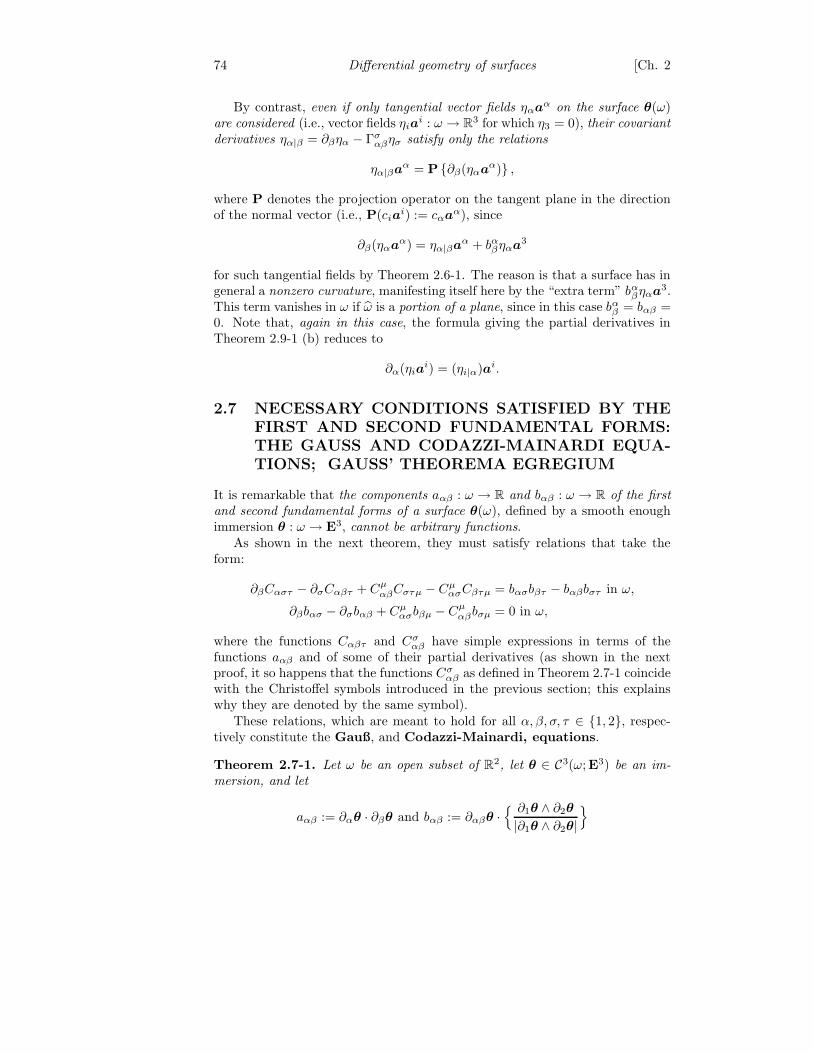
74 Differential geometry of surfaces [Ch. 2
By contrast, even if only tangential vector fields ηαaα on the surface θ(ω)
are considered (i.e., vector fields ηiai : ω → R3 for which η3 = 0), their covariant
derivatives ηα|β = ∂βηα − Γσαβησ satisfy only the relations
ηα|βaα = P ∂β(ηαa
α) ,
where P denotes the projection operator on the tangent plane in the directionof the normal vector (i.e., P(cia
i) := cαaα), since
∂β(ηαaα) = ηα|βa
α + bαβηαa
3
for such tangential fields by Theorem 2.6-1. The reason is that a surface has ingeneral a nonzero curvature, manifesting itself here by the “extra term” bα
βηαa3.
This term vanishes in ω if ω is a portion of a plane, since in this case bαβ = bαβ =
0. Note that, again in this case, the formula giving the partial derivatives inTheorem 2.9-1 (b) reduces to
∂α(ηiai) = (ηi|α)ai.
2.7 NECESSARY CONDITIONS SATISFIED BY THE
FIRST AND SECOND FUNDAMENTAL FORMS:
THE GAUSS AND CODAZZI-MAINARDI EQUA-
TIONS; GAUSS’ THEOREMA EGREGIUM
It is remarkable that the components aαβ : ω → R and bαβ : ω → R of the first
and second fundamental forms of a surface θ(ω), defined by a smooth enoughimmersion θ : ω → E3, cannot be arbitrary functions.
As shown in the next theorem, they must satisfy relations that take theform:
∂βCαστ − ∂σCαβτ + CµαβCστµ − Cµ
ασCβτµ = bασbβτ − bαβbστ in ω,
∂βbασ − ∂σbαβ + Cµασbβµ − Cµ
αβbσµ = 0 in ω,
where the functions Cαβτ and Cσαβ have simple expressions in terms of the
functions aαβ and of some of their partial derivatives (as shown in the nextproof, it so happens that the functions Cσ
αβ as defined in Theorem 2.7-1 coincidewith the Christoffel symbols introduced in the previous section; this explainswhy they are denoted by the same symbol).
These relations, which are meant to hold for all α, β, σ, τ ∈ 1, 2, respec-tively constitute the Gauß, and Codazzi-Mainardi, equations.
Theorem 2.7-1. Let ω be an open subset of R2, let θ ∈ C3(ω;E3) be an im-
mersion, and let
aαβ := ∂αθ · ∂βθ and bαβ := ∂αβθ · ∂1θ ∧ ∂2θ
|∂1θ ∧ ∂2θ|
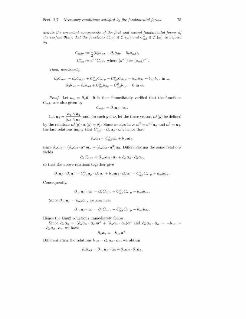
Sect. 2.7] Necessary conditions satisfied by the fundamental forms 75
denote the covariant components of the first and second fundamental forms of
the surface θ(ω). Let the functions Cαβτ ∈ C1(ω) and Cσαβ ∈ C1(ω) be defined
by
Cαβτ :=1
2(∂βaατ + ∂αaβτ − ∂τaαβ),
Cσαβ := aστCαβτ where (aστ ) := (aαβ)−1.
Then, necessarily,
∂βCαστ − ∂σCαβτ + CµαβCστµ − Cµ
ασCβτµ = bασbβτ − bαβbστ in ω,
∂βbασ − ∂σbαβ + Cµασbβµ − Cµ
αβbσµ = 0 in ω.
Proof. Let aα = ∂αθ. It is then immediately verified that the functionsCαβτ are also given by
Cαβτ = ∂αaβ · aτ .
Let a3 =a1 ∧ a2
|a1 ∧ a2|and, for each y ∈ ω, let the three vectors aj(y) be defined
by the relations aj(y) ·ai(y) = δji . Since we also have aβ = aαβaα and a3 = a3,
the last relations imply that Cσαβ = ∂αaβ · aσ , hence that
∂αaβ = Cσαβaσ + bαβa3,
since ∂αaβ = (∂αaβ · aσ)aσ + (∂αaβ · a3)a3. Differentiating the same relationsyields
∂σCαβτ = ∂ασaβ · aτ + ∂αaβ · ∂σaτ ,
so that the above relations together give
∂αaβ · ∂σaτ = Cµαβaµ · ∂σaτ + bαβa3 · ∂σaτ = Cµ
αβCστµ + bαβbστ .
Consequently,
∂ασaβ · aτ = ∂σCαβτ − CµαβCστµ − bαβbστ .
Since ∂ασaβ = ∂αβaσ , we also have
∂ασaβ · aτ = ∂βCαστ − CµασCβτµ − bασbβτ .
Hence the Gauß equations immediately follow.Since ∂αa3 = (∂αa3 · aσ)aσ + (∂αa3 · a3)a
3 and ∂αa3 · aσ = −bασ =−∂αaσ · a3, we have
∂αa3 = −bασaσ .
Differentiating the relations bαβ = ∂αaβ · a3, we obtain
∂σbαβ = ∂ασaβ · a3 + ∂αaβ · ∂σa3.
76 Differential geometry of surfaces [Ch. 2
This relation and the relations ∂αaβ = Cσαβaσ + bαβa3 and ∂αa3 = −bασa
σ
together imply that∂αaβ · ∂σa3 = −Cµ
αβbσµ.
Consequently,∂ασaβ · a3 = ∂σbαβ + Cµ
αβbσµ.
Since ∂ασaβ = ∂αβaσ, we also have
∂ασaβ · a3 = ∂βbασ + Cµασbβµ.
Hence the Codazzi-Mainardi equations immediately follow.
Remark. The vectors aα and aβ introduced above respectively form thecovariant and contravariant bases of the tangent plane to the surface θ(ω), theunit vector a3 = a3 is normal to the surface, and the functions aαβ are thecontravariant components of the first fundamental form (Sections 2.2 and 2.3).
As shown in the above proof, the Gauß and Codazzi-Mainardi equationsthus simply constitute a re-writing of the relations ∂ασaβ = ∂αβaσ in the formof the equivalent relations ∂ασaβ ·aτ = ∂αβaσ ·aτ and ∂ασaβ ·a3 = ∂αβaσ ·a3.
The functions
Cαβτ =1
2(∂βaατ + ∂αaβτ − ∂τaαβ) = ∂αaβ · aτ = Cβατ
andCσ
αβ = aστCαβτ = ∂αaβ · aσ = Cσβα
are the Christoffel symbols of the first, and second, kind. We recall thatthe same Christoffel symbols Cσ
αβ also naturally appeared in a different context(that of covariant differentiation; cf. Section 2.6).
Finally, the functions
Sταβσ := ∂βCαστ − ∂σCαβτ + CµαβCστµ − Cµ
ασCβτµ
are the covariant components of the Riemann curvature tensor of thesurface θ(ω).
Remark. Like the notation Cσαβ vs. Γp
ij , the notation Cαβτ is intended toavoid confusions with the “three-dimensional” Christoffel symbols Γijq intro-duced in Section 1.4.
Letting α = 2, β = 1, σ = 2, τ = 1 in the Gauß equations gives in particular
S1212 = det(bαβ).
Consequently, the Gaussian curvature at each point Θ(y) of the surface θ(ω)can be written as
1
R1(y)R2(y)=
S1212(y)
det(aαβ(y)), y ∈ ω,
Sect. 2.8] Existence of a surface with prescribed fundamental forms 77
since1
R1(y)R2(y)=
det(bαβ(y)
det(aαβ(y))(Theorem 2.5-1). By inspection of the function
S1212, we thus reach the astonishing conclusion that, at each point of the surface,
a notion involving the “curvature” of the surface, viz., the Gaussian curvature,
is entirely determined by the knowledge of the “metric” of the surface at the
same point, viz., the components of the first fundamental forms and their partialderivatives of order ≤ 2 at the same point! This startling conclusion naturallydeserves a theorem:
Theorem 2.7-2. Let ω be an open subset of R2, let θ ∈ C3(ω;E3) be an im-
mersion, let aαβ = ∂αθ ·∂βθ denote the covariant components of the first funda-
mental form of the surface θ(ω), and let the functions Cαβτ and S1212 be defined
by
Cαβτ :=1
2(∂βaατ + ∂αaβτ − ∂τaαβ),
S1212 :=1
2(2∂12a12 − ∂11a22 − ∂22a11) + aαβ(C12αC12β − C11αC22β).
Then, at each point θ(y) of the surface θ(ω), the principal curvatures 1R1(y)
and 1R2(y) satisfy
1
R1(y)R2(y)=
S1212(y)
det(aαβ(y)), y ∈ ω.
Theorem 2.7-2 constitutes the famed Theorema Egregium of Gauß [1828],so named by Gauß who had been himself astounded by his discovery.
2.8 EXISTENCE OF A SURFACE WITH PRESCRIBED
FIRST AND SECOND FUNDAMENTAL FORMS
Let M2, S2, and S2> denote the sets of all square matrices of order two, of all
symmetric matrices of order two, and of all symmetric, positive definite matricesof order two.
So far, we have considered that we are given an open set ω ⊂ R2 and asmooth enough immersion θ : ω → E3, thus allowing us to define the fields(aαβ) : ω → S
2> and (bαβ) : ω → S
2, where aαβ : ω → R and bαβ : ω → R
are the covariant components of the first and second fundamental forms of thesurface θ(ω) ⊂ E3.
Note that the immersion θ need not be injective in order that these matrixfields be well defined.
We now turn to the reciprocal questions:Given an open subset ω of R2 and two smooth enough matrix fields (aαβ) :
ω → S2> and (bαβ) : ω → S2, when are they the first and second fundamental
forms of a surface θ(ω) ⊂ E3, i.e., when does there exist an immersion θ : ω →E3 such that
aαβ := ∂αθ · ∂βθ and bαβ := ∂αβθ · ∂1θ ∧ ∂2θ
|∂1θ ∧ ∂2θ|
in ω?
78 Differential geometry of surfaces [Ch. 2
If such an immersion exists, to what extent is it unique?
The answers to these questions turn out to be remarkably simple: If ω is
simply-connected, the necessary conditions of Theorem 2.7-1, i.e., the Gauß
and Codazzi-Mainardi equations, are also sufficient for the existence of such an
immersion. If ω is connected, this immersion is unique up to isometries in E3.
Whether an immersion found in this fashion is injective is a different issue,which accordingly should be resolved by different means.
Following Ciarlet & Larsonneur [2001], we now give a self-contained, com-plete, and essentially elementary, proof of this well-known result. This proofamounts to showing that it can be established as a simple corollary to the fun-
damental theorem of three-dimensional differential geometry (Theorems 1.6-1and 1.7-1).
This proof has also the merit to shed light on the analogies (which cannotremain unnoticed!) between the assumptions and conclusions of both existence
results (compare Theorems 1.6-1 and 2.8-1) and both uniqueness results (com-pare Theorems 1.7-1 and 2.9-1).
A direct proof of the fundamental theorem of surface theory is given inKlingenberg [1973, Theorem 3.8.8], where the global existence of the mapping θis based on an existence theorem for ordinary differential equations, analogousto that used in part (ii) of the proof of Theorem 1.6-1. A proof of the “local”version of this theorem, which constitutes Bonnet’s theorem, is found in, e.g.,do Carmo [1976].
This result is another special case of the fundamental theorem of Rieman-
nian geometry alluded to in Section 1.6. We recall that this theorem asserts thata simply-connected Riemannian manifold of dimension p can be isometricallyimmersed into a Euclidean space of dimension (p + q) if and only if there existtensors satisfying together generalized Gauß, and Codazzi-Mainardi, equations
and that the corresponding isometric immersions are unique up to isometries inthe Euclidean space. A substantial literature has been devoted to this theoremand its various proofs, which usually rely on basic notions of Riemannian geom-etry, such as connections or normal bundles, and on the theory of differentialforms. See in particular the earlier papers of Janet [1926] and Cartan [1927]and the more recent references of Szczarba [1970], Tenenblat [1971], Jacobowitz[1982], and Szopos [2005].
Like the fundamental theorem of three-dimensional differential geometry,this theorem comprises two essentially distinct parts, a global existence result
(Theorem 2.8-1) and a uniqueness result (Theorem 2.9-1), the latter being alsocalled rigidity theorem. Note that these two results are established under dif-
ferent assumptions on the set ω and on the smoothness of the fields (aαβ) and(bαβ).
These existence and uniqueness results together constitute the fundamen-
tal theorem of surface theory.
Theorem 2.8-1. Let ω be a connected and simply-connected open subset of R2
and let (aαβ) ∈ C2(ω; S2>) and (bαβ) ∈ C2(ω; S2) be two matrix fields that satisfy
Sect. 2.8] Existence of a surface with prescribed fundamental forms 79
the Gauß and Codazzi-Mainardi equations, viz.,
∂βCαστ − ∂σCαβτ + CµαβCστµ − Cµ
ασCβτµ = bασbβτ − bαβbστ in ω,
∂βbασ − ∂σbαβ + Cµασbβµ − Cµ
αβbσµ = 0 in ω,
where
Cαβτ :=1
2(∂βaατ + ∂αaβτ − ∂τaαβ),
Cσαβ := aστCαβτ where (aστ ) := (aαβ)−1.
Then there exists an immersion θ ∈ C3(ω;E3) such that
aαβ = ∂αθ · ∂βθ and bαβ = ∂αβθ · ∂1θ ∧ ∂2θ
|∂1θ ∧ ∂2θ|
in ω.
Proof. The proof of this theorem as a corollary to Theorem 1.6-1 relieson the following elementary observation: Given a smooth enough immersionθ : ω → E3 and ε > 0, let the mapping Θ : ω × ]−ε, ε[ → E3 be defined by
Θ(y, x3) := θ(y) + x3a3(y) for all (y, x3) ∈ ω × ]−ε, ε[ ,
where a3 :=∂1θ ∧ ∂2θ
|∂1θ ∧ ∂2θ|, and let
gij := ∂iΘ · ∂jΘ.
Then an immediate computation shows that
gαβ = aαβ − 2x3bαβ + x23cαβ and gi3 = δi3 in ω × ]−ε, ε[ ,
where aαβ and bαβ are the covariant components of the first and second funda-mental forms of the surface θ(ω) and cαβ := aστbασbβτ .
Assume that the matrices (gij) constructed in this fashion are invertible,hence positive definite, over the set ω× ]−ε, ε[ (they need not be, of course; butthe resulting difficulty is easily circumvented; see parts (i) and (viii) below).Then the field (gij) : ω× ]−ε, ε[ → S3
> becomes a natural candidate for applyingthe “three-dimensional” existence result of Theorem 1.6-1, provided of coursethat the “three-dimensional” sufficient conditions of this theorem, viz.,
∂jΓikq − ∂kΓijq + ΓpijΓkqp − Γp
ikΓjqp = 0 in Ω,
can be shown to hold, as consequences of the “two-dimensional” Gauß and
Codazzi-Mainardi equations. That this is indeed the case is the essence of thepresent proof (see parts (i) to (vii)).
By Theorem 1.6-1, there then exists an immersion Θ : ω× ]−ε, ε[ → E3 thatsatisfies gij = ∂iΘ ·∂jΘ in ω× ]−ε, ε[. It thus remains to check that θ := Θ(·, 0)indeed satisfies (see part (ix))
aαβ = ∂αθ · ∂βθ and bαβ = ∂αβθ · ∂1θ ∧ ∂2θ
|∂1θ ∧ ∂2θ|
in ω.
80 Differential geometry of surfaces [Ch. 2
The actual implementation of this program essentially involves elementary,but sometimes lengthy, computations, which accordingly will be omitted for themost part; only the main intermediate results will be recorded.
For clarity, the proof is broken into nine parts, numbered (i) to (ix).
(i) Given two matrix fields (aαβ) ∈ C2(ω; S2>) and (bαβ) ∈ C2(ω; S2), let the
matrix field (gij) ∈ C2(ω × R; S3) be defined by
gαβ := aαβ − 2x3bαβ + x23cαβ and gi3 := δi3 in ω × R
(the variable y ∈ ω is omitted; x3 designates the variable in R), where
cαβ := bταbβτ and bτ
α := aστ bασ in ω.
Let ω0 be an open subset of R2 such that ω0 is a compact subset of ω. Then
there exists ε0 = ε0(ω0) > 0 such that the symmetric matrices (gij) are positive
definite at all points in Ω0, where
Ω0 := ω0 × ]−ε0, ε0[ .
Besides, the elements of the inverse matrix (gpq) are given in Ω0 by
gαβ =∑
n≥0
(n + 1)xn3aασ(Bn)β
σ and gi3 = δi3,
where
(B)βσ := bβ
σ and (Bn)βσ := bσ1
σ · · · bβσn−1
for n ≥ 2,
i.e., (Bn)βσ designates for any n ≥ 0 the element at the σ-th row and β-th
column of the matrix Bn. The above series are absolutely convergent in the
space C2(Ω0).Let a priori gαβ =
∑n≥0 xn
3hαβn where hαβ
n are functions of y ∈ ω0 only, so
that the relations gαβgβτ = δατ read
hαβ0 aβτ + x3(h
αβ1 aβτ − 2hαβ
0 bβτ )
+∑
n≥2
xn3 (hαβ
n aβτ − 2hαβn−1bβτ + hαβ
n−2cβτ ) = δατ .
It is then easily verified that the functions hαβn are given by
hαβn = (n + 1)aασ(Bn)β
σ , n ≥ 0,
so thatgαβ =
∑
n≥0
(n + 1)xn3 aασbσ1
σ · · · bβσn−1
.
It is clear that such a series is absolutely convergent in the space C2(ω0 ×[−ε0, ε0]) if ε0 > 0 is small enough.

Sect. 2.8] Existence of a surface with prescribed fundamental forms 81
(ii) The functions Cσαβ being defined by
Cσαβ := aστCαβτ ,
where
(aστ ) := (aαβ)−1 and Cαβτ :=1
2(∂βaατ + ∂αaβτ − ∂τaαβ),
define the functions
bτα|β := ∂βbτ
α + Cτβµbµ
α − Cµαβbτ
µ,
bαβ|σ := ∂σbαβ − Cµασbβµ − Cµ
βσbαµ = bβα|σ.
Then
bτα|β = aστ bασ|β and bασ|β = aστ bτ
α|β .
Furthermore, the assumed Codazzi-Mainardi equations imply that
bτα|β = bτ
β|α and bασ|β = bαβ|σ.
The above relations follow from straightforward computations based on thedefinitions of the functions bτ
α|β and bαβ|σ. They are recorded here because theyplay a pervading role in the subsequent computations.
(iii) The functions gij ∈ C2(Ω0) and gij ∈ C2(Ω0) being defined as in part (i),define the functions Γijq ∈ C1(Ω0) and Γp
ij ∈ C1(Ω0) by
Γijq :=1
2(∂jgiq + ∂igjq − ∂qgij) and Γp
ij := gpqΓijq .
Then the functions Γijq = Γjiq and Γpij = Γp
ji have the following expressions :
Γαβσ = Cαβσ − x3(bτα|βaτσ + 2Cτ
αβbτσ) + x23(b
τα|βbτσ + Cτ
αβcτσ),
Γαβ3 = −Γα3β = bαβ − x3cαβ ,
Γα33 = Γ3β3 = Γ33q = 0,
Γσαβ = Cσ
αβ −∑
n≥0xn+1
3 bτα|β(Bn)σ
τ ,
Γ3αβ = bαβ − x3cαβ ,
Γβα3 = −
∑n≥0
xn3 (Bn+1)β
α,
Γ33β = Γp
33 = 0,
where the functions cαβ, (Bn)στ , and bτ
α|β are defined as in parts (i) and (ii).All computations are straightforward. We simply point out that the assumed
Codazzi-Mainardi equations are needed to conclude that the factor of x3 in thefunction Γαβσ is indeed that announced above. We also note that the compu-tation of the factor of x2
3 in Γαβσ relies in particular on the easily establishedrelations
∂αcβσ = bτβ |αbστ + bµ
σ |αbµβ + Cµαβcσµ + Cµ
ασcβµ.
82 Differential geometry of surfaces [Ch. 2
(iv) The functions Γijq ∈ C1(Ω0) and Γpij ∈ C1(Ω0) being defined as in
part (iii), define the functions Rqijk ∈ C0(Ω0) by
Rqijk := ∂jΓikq − ∂kΓijq + ΓpijΓkqp − Γp
ikΓjqp.
Then, in order that the relations
Rqijk = 0 in Ω0
hold, it is sufficient that
R1212 = 0, Rα2β3 = 0, Rα3β3 = 0 in Ω0.
The above definition of the functions Rqijk and that of the functions Γijq
and Γpij (part (iii)) together imply that, for all i, j, k, q,
Rqijk = Rjkqi = −Rqikj ,
Rqijk = 0 if j = k or q = i.
Consequently, the relation R1212 = 0 implies that Rαβστ = 0, the relationsRα2β3 = 0 imply that Rqijk = 0 if exactly one index is equal to 3, and finally,the relations Rα3β3 = 0 imply that Rqijk = 0 if exactly two indices are equalto 3.
(v) The functions
Rα3β3 := ∂βΓ33α − ∂3Γ3βα + Γp3βΓ3αp − Γp
33Γβαp
satisfy
Rα3β3 = 0 in Ω0.
These relations immediately follow from the expressions found in part (iii)for the functions Γijq and Γp
ij . Note that neither the Gauß equations nor theCodazzi-Mainardi equations are needed here.
(vi) The functions
Rα2β3 := ∂βΓ23α − ∂3Γ2βα + Γp2βΓ3αp − Γp
23Γβαp
satisfy
Rα2β3 = 0 in Ω0.
The definitions of the functions gαβ (part (i)) and Γijq (part (iii)) show that
∂βΓ23α − ∂3Γ2βα = (∂2bαβ − ∂αb2β) + x3(∂αc2β − ∂2cαβ).
Then the expressions found in part (iii) show that
Γp2βΓ3αp − Γp
23Γβαp = Γσ3αΓ2βσ − Γσ
23Γαβσ
= Cσαβb2σ − Cσ
2βbασ
+ x3(bσ2 |βbασ − bσ
α|βb2σ + Cσ2βcασ − Cσ
αβc2σ),

Sect. 2.8] Existence of a surface with prescribed fundamental forms 83
and the relations Rα3β3 = 0 follow by making use of the relations
∂αcβσ = bτβ|αbστ + bµ
σ|αbµβ + Cµαβcσµ + Cµ
ασcβµ
together with the relations
∂2bαβ − ∂αb2β + Cσαβb2σ − Cσ
2βbασ = 0,
which are special cases of the assumed Codazzi-Mainardi equations.
(vii) The function
R1212 := ∂1Γ221 − ∂2Γ211 + Γp21Γ21p − Γp
22Γ11p
satisfies
R1212 = 0 in Ω0.
The computations leading to this relation are fairly lengthy and they requiresome care. We simply record the main intermediary steps, which consist inevaluating separately the various terms occurring in the function R1212 rewrittenas
R1212 = (∂1Γ221 − ∂2Γ211) + (Γσ12Γ12σ − Γσ
11Γ22σ) + (Γ123Γ123 − Γ113Γ223).
First, the expressions found in part (iii) for the functions Γαβ3 easily yield
Γ123Γ123 − Γ113Γ223 = (b212 − b11b22)
+ x3(b11c22 − 2b12c12 + b22c11) + x23(c
212 − c11c22).
Second, the expressions found in part (iii) for the functions Γαβσ and Γσαβ
yield, after some manipulations:
Γσ12Γ12σ − Γσ
11Γ22σ = (Cσ12C
τ12 − Cσ
11Cτ22)aστ
+ x3(Cσ11b
τ2 |2 − 2Cσ
12bτ1 |2 + Cσ
22bτ1 |1)aστ
+ 2(Cσ11C
τ22 − Cσ
12Cτ12)bστ
+ x23bσ
1 |1bτ2 |2 − bσ
1 |2bτ1 |2)aστ
+ (Cσ11b
τ2 |2 − 2Cσ
12bτ1 |2 + Cσ
22bτ1 |1)bστ
+ (Cσ11C
τ22 − Cσ
12Cτ12)cστ.
Third, after somewhat delicate computations, which in particular make useof the relations established in part (ii) about the functions bτ
α|β and bαβ|σ, it isfound that
∂1Γ221 − ∂2Γ211 = ∂1C221 − ∂2C211
− x3S1212bαα + (Cσ
11bτ2 |2 − 2Cσ
12bτ1 |2 + Cσ
22bτ1 |1)aστ
+ 2(Cσ11C
τ22 − Cσ
12Cτ12)bστ
+ x23Sστ12b
σ1 bτ
2 + (bσ1 |1bτ
2 |2 − bσ1 |2bτ
1 |2)aστ
+ (Cσ11b
τ2 |2 − 2Cσ
12bτ1 |2 + Cσ
22bτ1 |1)bσ
+ (Cσ11C
τ22 − Cσ
12Cτ12)cστ,
84 Differential geometry of surfaces [Ch. 2
where the functions
Sταβσ := ∂βCαστ − ∂σCαβτ + CµαβCστµ − Cµ
ασCβτµ
are precisely those appearing in the left-hand sides of the Gauß equations.It is then easily seen that the above equations together yield
R1212 = S1212 − (b11b22 − b12b12)− x3S1212 − (b11b22 − b12b12)b
αα
+ x23Sστ12b
σ1 bτ
2 + (c12c12 − c11c22).
Since
Sστ12bσ1 bτ
2 = S1212(b11b
22 − b2
1b12),
c12c12 − c11c22 = (b11b12 − b11b22)(b11b
22 − b2
1b12),
it is finally found that the function R1212 has the following remarkable expres-sion:
R1212 = S1212 − (b11b22 − b12b12)1− x3(b11 + b2
2) + x23(b
11b
22 − b2
1b12).
By the assumed Gauß equations,
S1212 = b11b22 − b12b12.
Hence R1212 = 0 as announced.
(viii) Let ω be a connected and simply-connected open subset of R2. Then
there exist open subsets ω`, ` ≥ 0, of R2 such that ω` is a compact subset of ωfor each ` ≥ 0 and
ω =⋃
`≥0
ω`.
Furthermore, for each ` ≥ 0, there exists ε` = ε`(ω`) > 0 such that the symmet-
ric matrices (gij) are positive definite at all points in Ω`, where
Ω` := ω` × ]−ε`, ε`[ .
Finally, the open set
Ω :=⋃
`≥0
Ω`
is connected and simply-connected.
Let ω`, ` ≥ 0, be open subsets of ω with compact closures ω` ⊂ ω such thatω =
⋃`≥0 ω`. For each `, a set Ω` := ω` × ]−ε`, ε`[ can then be constructed in
the same way that the set Ω0 was constructed in part (i).It is clear that the set Ω :=
⋃`≥0 Ω` is connected. To show that Ω is simply-
connected, let γ be a loop in Ω, i.e., a mapping γ ∈ C0([0, 1]; R3) that satisfies
γ(0) = γ(1) and γ(t) ∈ Ω for all 0 ≤ t ≤ 1.
Sect. 2.8] Existence of a surface with prescribed fundamental forms 85
Let the projection operator π : Ω → ω be defined by π(y, x3) = y for all(y, x3) ∈ Ω, and let the mapping ϕ0 : [0, 1]× [0, 1] → R3 be defined by
ϕ0(t, λ) := (1 − λ)γ(t) + λπ(γ(t)) for all 0 ≤ t ≤ 1, 0 ≤ λ ≤ 1.
Then ϕ0 is a continuous mapping such that ϕ0([0, 1]×[0, 1]) ⊂ Ω, by definition ofthe set Ω. Furthermore, ϕ0(t, 0) = γ(t) and ϕ0(t, 1) = π(γ(t)) for all t ∈ [0, 1].
The mapping
γ := π γ ∈ C0([0, 1]; R2)
is a loop in ω since γ(0) = π(γ(0)) = π(γ(1)) = γ(1) and γ(t) ∈ ω forall 0 ≤ t ≤ 1. Since ω is simply connected, there exist a mapping ϕ1 ∈C0([0, 1] × [0, 1]; R2) and a point y0 ∈ ω such that
ϕ1(t, 1) = γ and ϕ1(t, 2) = y0 for all 0 ≤ t ≤ 1
and
ϕ1(t, λ) ∈ ω for all 0 ≤ t ≤ 1, 1 ≤ λ ≤ 2.
Then the mapping ϕ ∈ C0([0, 1] × [0, 2]; R3) defined by
ϕ(t, λ) = ϕ0(t, λ) for all 0 ≤ t ≤ 1, 0 ≤ λ ≤ 1,ϕ(t, λ) = ϕ1(t, λ) for all 0 ≤ t ≤ 1, 1 ≤ λ ≤ 2,
is a homotopy in Ω that reduces the loop γ to the point (y0, 0) ∈ Ω. Hence theset Ω is simply-connected.
(ix) By parts (iv) to (viii), the functions Γijq ∈ C1(Ω) and Γpij ∈ C1(Ω)
constructed as in part (iii) satisfy
∂jΓikq − ∂kΓijq + ΓpijΓkqp − Γp
ikΓjqp = 0
in the connected and simply-connected open set Ω. By Theorem 1.6-1, there thus
exists an immersion Θ ∈ C3(Ω;E3) such that
gij = ∂iΘ · ∂jΘ in Ω,
where the matrix field (gij) ∈ C2(Ω; S3>) is defined by
gαβ = aαβ − 2x3bαβ + x23cαβ and gi3 = δi3 in Ω.
Then the mapping θ ∈ C3(ω;E3) defined by
θ(y) = Θ(y, 0) for all y ∈ ω,
satisfies
aαβ = ∂αθ · ∂βθ and bαβ = ∂αβθ · ∂1θ ∧ ∂2θ
|∂1θ ∧ ∂2θ|
in ω.
86 Differential geometry of surfaces [Ch. 2
Let gi := ∂iΘ. Then ∂33Θ = ∂3g3 = Γp33gp = 0; cf. part (iii). Hence there
exists a mapping θ1 ∈ C3(ω;E3) such that
Θ(y, x3) = θ(y) + x3θ1(y) for all (y, x3) ∈ Ω,
and consequently, gα = ∂αθ+x3∂αθ1 and g3 = θ1. The relations gi3 = gi ·g3 =
δi3 (cf. part (i)) then show that
(∂αθ + x3∂αθ1) · θ1 = 0 and θ1 · θ1 = 1.
These relations imply that ∂αθ · θ1 = 0. Hence either θ1 = a3 or θ1 = −a3
in ω, where
a3 :=∂1θ ∧ ∂2θ
|∂1θ ∧ ∂2θ|.
But θ1 = −a3 is ruled out since
∂1θ ∧ ∂2θ · θ1 = det(gij)|x3=0 > 0.
Noting that
∂αθ · a3 = 0 implies ∂αθ · ∂βa3 = −∂αβθ · a3,
we obtain, on the one hand,
gαβ = (∂αθ + x3∂αa3) · (∂βθ + x3∂βa3)
= ∂αθ · ∂βθ − 2x3∂αβθ · a3 + x23∂αa3 · ∂βa3 in Ω.
Since, on the other hand,
gαβ = aαβ − 2x3bαβ + x23cαβ in Ω
by part (i), we conclude that
aαβ = ∂αθ · ∂βθ and bαβ = ∂αβθ · a3 in ω,
as desired. This completes the proof.
Remarks. (1) The functions cαβ = bταbβτ = ∂αa3 ·∂βa3 introduced in part (i)
are the covariant components of the third fundamental form of the surface θ(ω).(2) The series expansion gαβ =
∑n≥0(n + 1)xn
3 aασ(Bn)βσ found in part (i)
is known; cf., e.g., Naghdi [1972].(3) The Gauß equations are used only once in the above proof, for showing
that R1212 = 0 in part (vii).
The definitions of the functions Cσαβ and Cαβτ imply that the sixteen Gauß
equations are satisfied if and only if they are satisfied for α = 1, β = 2,σ = 1, τ = 2 and that the Codazzi-Mainardi equations are satisfied if and only
Sect. 2.9] Uniqueness of surfaces with the same fundamental forms 87
if they are satisfied for α = 1, β = 2, σ = 1 and α = 1, β = 2, σ = 2 (otherchoices of indices with the same properties are clearly possible).
In other words, the Gauß equations and the Codazzi-Mainardi equations infact reduce to one and two equations, respectively.
The regularity assumptions made in Theorem 2.8-1 on the matrix fields (aαβ)and (bαβ) can be significantly relaxed in several ways. First, C. Mardare [2003b]has shown by means of an ad hoc, but not trivial, modification of the proofgiven here, that the existence of an immersion θ ∈ C3(ω;E3) still holds underthe weaker (but certainly more natural, in view of the regularity of the result-ing immersion θ) assumption that (bαβ) ∈ C1(ω; S2), all other assumptions ofTheorem 2.8-1 holding verbatim.
In fact, Hartman & Wintner [1950] have shown the stronger result that theexistence theorem still holds if (aαβ) ∈ C1(ω; S2
>) and (bαβ) ∈ C0(ω; S2), with aresulting mapping θ in the space C2(ω;E3). Their result has been itself super-seded by that of S. Mardare [2004], which asserts that if (aαβ) ∈ W 1,∞
loc (ω; S2>)
and (bαβ) ∈ L∞loc(ω; S2) are two matrix fields that satisfy the Gauß and Codazzi-
Mainardi equations in the sense of distributions, then there exists a mappingθ ∈ W 2,∞
loc (ω) such that (aαβ) and (bαβ) are the fundamental forms of the sur-face θ(ω).
2.9 UNIQUENESS UP TO ISOMETRIES OF SURFACES
WITH THE SAME FUNDAMENTAL FORMS
In Section 2.8, we have established the existence of an immersion θ : ω ⊂ R2 →E3 giving rise to a surface θ(ω) with prescribed first and second fundamentalforms, provided these forms satisfy ad hoc sufficient conditions. We now turnto the question of uniqueness of such immersions.
This is the object of the next theorem, which constitutes another rigidity
theorem, called the rigidity theorem for surfaces. Like its “three-dimensionalcounterpart” (Theorem 1.7-1), it asserts that, if two immersions θ ∈ C2(ω;E3)
and θ ∈ C2(ω;E3) share the same fundamental forms, then the surface θ(ω)is obtained by subjecting the surface θ(ω) to a rotation (represented by anorthogonal matrix Q with det Q = 1), then by subjecting the rotated surfaceto a translation (represented by a vector c). Such a “rigid” transformation isthus an isometry in E3.
As shown by Ciarlet & Larsonneur [2001] (whose proof is adapted here),the issue of uniqueness can be resolved as a corollary to its “three-dimensionalcounterpart”, like the issue of existence. We recall that O3 denotes the set of allorthogonal matrices of order three and that O3
+ = Q ∈ O3; detQ = 1 denotesthe set of all 3 × 3 rotations.
Theorem 2.9-1. Let ω be a connected open subset of R2 and let θ ∈ C2(ω;E3)
and θ ∈ C2(ω;E3) be two immersions such that their associated first and second
fundamental forms satisfy (with self-explanatory notations)
aαβ = aαβ and bαβ = bαβ in ω.

88 Differential geometry of surfaces [Ch. 2
Then there exist a vector c ∈ E3 and a rotation Q ∈ O3+ such that
θ(y) = c+ Qθ(y) for all y ∈ ω.
Proof. Arguments similar to those used in parts (i) and (viii) of the proofof Theorem 2.8-1 show that there exist open subsets ω` of ω and real numbersε` > 0, ` ≥ 0, such that the symmetric matrices (gij) defined by
gαβ := aαβ − 2x3bαβ + x23cαβ and gi3 = δi3,
where cαβ := aστ bασbβτ , are positive definite in the set
Ω :=⋃
`≥0
ω` × ]−ε`, ε`[ .
The two immersions Θ ∈ C1(Ω;E3) and Θ ∈ C1(Ω;E3) defined by (withself-explanatory notations)
Θ(y, x3) := θ(y) + x3a3(y) and Θ(y, x3) := θ(y) + x3a3(y)
for all (y, x3) ∈ Ω therefore satisfy
gij = gij in Ω.
By Theorem 1.7-1, there exist a vector c ∈ E3 and an orthogonal matrixQ ∈ O3 such that
Θ(y, x3) = c+ QΘ(y, x3) for all (y, x3) ∈ Ω.
Hence, on the one hand,
det ∇Θ(y, x3) = detQ det ∇Θ(y, x3) for all (y, x3) ∈ Ω.
On the other hand, a simple computation shows that
det ∇Θ(y, x3) =√
det(aαβ(y)1− x3(b11 + b2
2)(y) + x23(b
11b
22 − b2
1b12)(y)
for all (y, x3) ∈ Ω, where
bβα(y) := aβσ(y)bασ(y), y ∈ ω,
so thatdet ∇Θ(y, x3) = det ∇Θ(y, x3) for all (y, x3) ∈ Ω.
Therefore detQ = 1, which shows that the matrix Q ∈ O3 is in fact arotation. The conclusion then follows by letting x3 = 0 in the relation
Θ(y, x3) = c+ QΘ(y, x3) for all (y, x3) ∈ Ω.
Sect. 2.9] Uniqueness of surfaces with the same fundamental forms 89
As a preparation to our next result, we note that the second fundamentalform of the surface θ(ω) can still be defined under the weaker assumptions that
θ ∈ C1(ω;E3) and a3 =a1 ∧ a2
|a1 ∧ a2|∈ C1(ω;E3), by means of the definition
bαβ := −aα · ∂βa3,
which evidently coincides with the usual one when θ ∈ C2(ω;E3).
Theorem 2.9-1 constitutes the “classical” rigidity theorem for surfaces, in thesense that both immersions θ and θ are assumed to be in the space C2(ω;E3).
Following Ciarlet & C. Mardare [2004a], we now show that a similar re-
sult holds under the assumptions that θ ∈ H1(ω;E3) and a3 :=a1 ∧ a2
|a1 ∧ a2|∈
H1(ω;E3) (with self-explanatory notations). Naturally, our first task will be toverify that the vector field a3, which is not necessarily well defined a.e. in ω foran arbitrary mapping θ ∈ H1(ω;E3), is nevertheless well defined a.e. in ω for
those mappings θ that satisfy the assumptions of the next theorem. This factwill in turn imply that the functions bαβ := −aα ·∂β a3 are likewise well defineda.e. in ω.
Theorem 2.9-2. Let ω be a connected open subset of R2 and let θ ∈ C1(ω;E3)be an immersion that satisfies a3 ∈ C1(ω;E3). Assume that there exists a vector
field θ ∈ H1(ω;E3) that satisfies
aαβ = aαβ a.e. in ω, a3 ∈ H1(ω;E3), and bαβ = bαβ a.e. in ω.
Then there exist a vector c ∈ E3 and a matrix Q ∈ O3+ such that
θ(y) = c+ Qθ(y) for almost all y ∈ ω.
Proof. The proof essentially relies on the extension to a Sobolev space settingof the “three-dimensional” rigidity theorem established in Theorem 1.7-3.
(i) To begin with, we record several technical preliminaries.
First, we observe that the relations aαβ = aαβ a.e. in ω and the assumptionthat θ ∈ C1(ω;E3) is an immersion together imply that
|a1 ∧ a2| =√
det(aαβ) =√
det(aαβ) > 0 a.e. in ω.
Consequently, the vector field a3, and thus the functions bαβ, are well defined
a.e. in ω.
Second, we establish that
bαβ = bβα in ω and bαβ = bβα a.e. in ω,
90 Differential geometry of surfaces [Ch. 2
i.e., that aα · ∂βa3 = aβ · ∂αa3 in ω and aα · ∂βa3 = aβ · ∂αa3 a.e. in ω. Tothis end, we note that either the assumptions θ ∈ C1(ω;E3) and a3 ∈ C1(ω;E3)together, or the assumptions θ ∈ H1(ω;E3) and a3 ∈ H1(ω;E3) together, implythat aα · ∂βa3 = ∂αθ · ∂βa3 ∈ L1
loc(ω), hence that ∂αθ · ∂βa3 ∈ D′(ω).Given any ϕ ∈ D(ω), let U denote an open subset of R2 such that supp ϕ ⊂ U
and U is a compact subset of ω. Denoting by X′〈·, ·〉X the duality pairingbetween a topological vector space X and its dual X ′, we have
D′(ω)〈∂αθ · ∂βa3, ϕ〉D(ω) =
∫
ω
ϕ∂αθ · ∂βa3 dy
=
∫
ω
∂αθ · ∂β(ϕa3)dy −∫
ω
(∂βϕ)∂αθ · a3 dy.
Observing that ∂αθ · a3 = 0 a.e. in ω and that
−∫
ω
∂αθ · ∂β(ϕa3)dy = −∫
U
∂αθ · ∂β(ϕa3)dy
= H−1(U ;E3)〈∂β(∂αθ), ϕa3〉H1
0(U ;E3),
we reach the conclusion that the expression D′(ω)〈∂αθ·∂βa3, ϕ〉D(ω) is symmetricwith respect to α and β since ∂αβθ = ∂βαθ in D′(U). Hence ∂αθ · ∂βa3 =∂βθ · ∂αa3 in L1
loc(ω), and the announced symmetries are established.Third, let
cαβ := ∂αa3 · ∂βa3 and cαβ := ∂αa3 · ∂βa3.
Then we claim that cαβ = cαβ a.e. in ω. To see this, we note that the matrixfields (aαβ) := (aαβ)−1 and (aαβ) := (aαβ)−1 are well defined and equal a.e. inω since θ is an immersion and aαβ = aαβ a.e. in ω. The formula of Weingarten
(Section 2.6) can thus be applied a.e. in ω, showing that cαβ = aστ bσαbτβ a.e.in ω.
The assertion then follows from the assumptions bαβ = bαβ a.e. in ω.
(ii) Starting from the set ω and the mapping θ (as given in the statementof Theorem 2.9-2), we next construct a set Ω and a mapping Θ that satisfy the
assumptions of Theorem 1.7-2. More precisely, let
Θ(y, x3) := θ(y) + x3a3(y) for all (y, x3) ∈ ω × R.
Then the mapping Θ := ω × R → E3 defined in this fashion is clearly continu-ously differentiable on ω × R and
det ∇Θ(y, x3) =√
det(aαβ(y))1− x3(b11 + b2
2)(y) + x23(b
11b
22 − b2
1b12)(y)
for all (y, x3) ∈ ω × R, where
bβα(y) := aβσ(y)bασ(y), y ∈ ω.
Let ωn, n ≥ 0, be open subsets of R2 such that ωn is a compact subset of ωand ω =
⋃n≥0 ωn. Then the continuity of the functions aαβ, aαβ , bαβ and the
Sect. 2.10] Uniqueness of surfaces with the same fundamental forms 91
assumption that θ is an immersion together imply that, for each n ≥ 0, thereexists εn > 0 such that
det ∇Θ(y, x3) > 0 for all (y, x3) ∈ ωn × [−εn, εn].
Besides, there is no loss of generality in assuming that εn ≤ 1 (this propertywill be used in part (iii)).
Let thenΩ :=
⋃
n≥0
(ωn × ]−εn, εn[).
Then it is clear that Ω is a connected open subset of R3 and that the mapping
Θ ∈ C1(Ω;E3) satisfies det ∇Θ > 0 in Ω.
Finally, note that the covariant components gij ∈ C0(Ω) of the metric tensorfield associated with the mapping Θ are given by (the symmetries bαβ = bβα
established in (i) are used here)
gαβ = aαβ − 2x3bαβ + x23cαβ , gα3 = 0, g33 = 1.
(iii) Starting with the mapping θ (as given in the statement of Theorem
2.9-2), we construct a mapping Θ that satisfies the assumptions of Theorem
1.7-2. To this end, we define a mapping Θ : Ω → E3 by letting
Θ(y, x3) := θ(y) + x3a3(y) for all (y, x3) ∈ Ω,
where the set Ω is defined as in (ii). Hence Θ ∈ H1(Ω;E3), since Ω ⊂ ω×]−1, 1[.
Besides, det ∇Θ = det ∇Θ a.e. in Ω since the functions bβα := aβσ bασ, which are
well defined a.e. in ω, are equal, again a.e. in ω, to the functions bβα. Likewise, the
components gij ∈ L1(Ω) of the metric tensor field associated with the mapping
Θ satisfy gij = gij a.e. in Ω since aαβ = aαβ and bαβ = bαβ a.e. in ω byassumption and cαβ = cαβ a.e. in ω by part (i).
(iv) By Theorem 1.7-2, there exist a vector c ∈ E3 and a matrix Q ∈ O3+
such that
θ(y) + x3a3(y) = c+ Q(θ(y) + x3a3(y)) for almost all (y, x3) ∈ Ω.
Differentiating with respect to x3 in this equality between functions in H1(Ω;E3)
shows that a3(y) = Qa3(y) for almost all y ∈ ω. Hence θ(y) = c+ Qθ(y) foralmost all y ∈ ω as announced.
Remarks. (1) The existence of θ ∈ H1(ω;E3) satisfying the assumptions
of Theorem 2.9-2 implies that θ ∈ C1(ω;E3) and a3 ∈ C1(ω;E3), and thatθ ∈ H1(ω;E3) and a3 ∈ H1(ω;E3).
(2) It is easily seen that the conclusion of Theorem 2.9-2 is still valid if the
assumptions θ ∈ H1(ω;E3) and a3 ∈ H1(ω;E3) are replaced by the weaker
assumptions θ ∈ H1loc(ω;E3) and a3 ∈ H1
loc(ω;E3).
92 Differential geometry of surfaces [Ch. 2
2.10 CONTINUITY OF A SURFACE AS A FUNCTION
OF ITS FUNDAMENTAL FORMS
Let ω be a connected and simply-connected open subset of R2. Together, The-orems 2.8-1 and 2.9-1 establish the existence of a mapping F that associatesto any pair of matrix fields (aαβ) ∈ C2(ω; S2
>) and (bαβ) ∈ C2(ω; S2) satis-fying the Gauß and Codazzi-Mainardi equations in ω a well-defined elementF ((aαβ), (bαβ)) in the quotient set C3(ω;E3)/R, where (θ, θ) ∈ R means that
there exists a vector c ∈ E3 and a rotation Q ∈ O3+ such that θ(y) = c+Qθ(y)
for all y ∈ ω.A natural question thus arises as to whether there exist ad hoc topologies on
the space C2(ω; S2) × C2(ω; S2) and on the quotient set C3(ω;E3)/R such thatthe mapping F defined in this fashion is continuous.
Equivalently, is a surface a continuous function of its fundamental forms?
The purpose of this section, which is based on Ciarlet [2003], is to providean affirmative answer to the above question, through a proof that relies in anessential way on the solution to the analogous problem in dimension three givenin Section 1.8.
Such a question is not only relevant to surface theory, but it also findsits source in two-dimensional nonlinear shell theories, where the stored energy
functions are often functions of the first and second fundamental forms of the
unknown deformed middle surface (for an overview of nonlinear shell theories,see, e.g., Ciarlet [2000]). For instance, the well-known stored energy functionwK proposed by Koiter [1966, Equations (4.2), (8.1), and (8.3)] for modelingnonlinearly elastic shells made with a homogeneous and isotropic elastic materialtakes the form:
wK =ε
2aαβστ (aστ−aστ )(aαβ−aαβ) +
ε3
6aαβστ (bστ−bστ )(bαβ−bαβ),
where 2ε is the thickness of the shell,
aαβστ :=4λµ
λ + 2µaαβaστ + 2µ(aασaβτ+aατaβσ),
λ > 0 and µ > 0 are the two Lame constants of the constituting material, aαβ
and bαβ are the covariant components of the first and second fundamental formsof the given undeformed middle surface, (aαβ) = (aαβ)−1, and finally aαβ and
bαβ are the covariant components of the first and second fundamental forms ofthe unknown deformed middle surface.
An inspection of the above stored energy functions thus suggests a temptingapproach to shell theory, where the functions aαβ and bαβ would be regarded
as the primary unknowns in lieu of the customary (Cartesian or curvilinear)components of the displacement. In such an approach, the unknown componentsaαβ and bαβ must naturally satisfy the classical Gauß and Codazzi-Mainardi
equations in order that they actually define a surface.To begin with, we introduce the following two-dimensional analogs to the
notations used in Section 1.8. Let ω be an open subset of R3. The notation κ b ω

Sect. 2.10] A surface as a function of its fundamental forms 93
means that κ is a compact subset of ω. If f ∈ C`(ω; R) or θ ∈ C`(ω;E3), ` ≥ 0,and κ b ω, we let
‖f‖`,κ := supy∈κ|α|≤`
|∂αf(y)| , ‖θ‖`,κ := supy∈κ|α|≤`
|∂αθ(y)|,
where ∂α stands for the standard multi-index notation for partial derivatives and|·| denotes the Euclidean norm in the latter definition. If A ∈ C`(ω; M3), ` ≥ 0,and κ b ω, we likewise let
‖A‖`,κ = supn y∈κ|α|≤`
|∂αA(y)|,
where |·| denotes the matrix spectral norm.The next sequential continuity result constitutes the key step towards estab-
lishing the continuity of a surface as a function of its two fundamental forms inad hoc metric spaces (see Theorem 2.10-2).
Theorem 2.10-1. Let ω be a connected and simply-connected open subset of R2.
Let (aαβ) ∈ C2(ω; S2>) and (bαβ) ∈ C2(ω; S2) be matrix fields satisfying the Gauß
and Codazzi-Mainardi equations in ω and let (anαβ) ∈ C2(ω; S2
>) and (bnαβ) ∈
C2(ω; S2) be matrix fields satisfying for each n ≥ 0 the Gauß and Codazzi-
Mainardi equations in ω. Assume that these matrix fields satisfy
limn→∞
‖anαβ−aαβ‖2,κ = 0 and lim
n→∞‖bn
αβ−bαβ‖2,κ = 0 for all κ b ω.
Let θ ∈ C3(ω;E3) be any mapping that satisfies
aαβ = ∂αθ · ∂βθ and bαβ = ∂αβθ · ∂1θ ∧ ∂2θ
|∂1θ ∧ ∂2θ|
in ω
(such mappings exist by Theorem 2.8-1). Then there exist mappings θn ∈C3(ω;E3) satisfying
anαβ = ∂αθ
n · ∂βθn and bn
αβ = ∂αβθn ·
∂1θn ∧ ∂2θ
n
|∂1θn ∧ ∂2θ
n|
in ω, n ≥ 0,
such that
limn→∞
‖θn−θ‖3,κ = 0 for all κ b ω.
Proof. For clarity, the proof is broken into five parts.
(i) Let the matrix fields (gij) ∈ C2(ω×R; S3) and (gnij) ∈ C2(ω×R; S3), n ≥ 0,
be defined by
gαβ := aαβ − 2x3bαβ + x23cαβ and gi3 := δi3,
gnαβ := an
αβ − 2x3bnαβ + x2
3cnαβ and gn
i3 := δi3, n ≥ 0

94 Differential geometry of surfaces [Ch. 2
(the variable y ∈ ω is omitted, x3 designates the variable in R), where
cαβ := bταbβτ , bτ
α := aστ bασ , (aστ ) := (aαβ)−1,
cnαβ := bτ,n
α bnβτ , bτ,n
α := aστ,nbnασ , (aστ,n) := (an
αβ)−1, n ≥ 0.
Let ω0 be an open subset of R2 such that ω0 b ω. Then there exists ε0 =ε0(ω0) > 0 such that the symmetric matrices
C(y, x3) := (gij(y, x3)) and Cn(y, x3) := (gnij(y, x3)), n ≥ 0,
are positive definite at all points (y, x3) ∈ Ω0, where
Ω0 := ω0 × ]−ε0, ε0[ .
The matrices C(y, x3) ∈ S3 and Cn(y, x3) ∈ S3 are of the form (the notationsare self-explanatory):
C(y, x3) = C0(y) + x3C1(y) + x23C2(y),
Cn(y, x3) = Cn0 (y) + x3C
n1 (y) + x2
3Cn2 (y), n ≥ 0.
First, it is easily deduced from the matrix identity B = A(I + A−1(B−A))and the assumptions limn→∞ ‖an
αβ−aαβ‖0,ω0= 0 and limn→∞ ‖bn
αβ−bαβ‖0,ω0=
0 that there exists a constant M such that
‖(Cn0 )−1‖0,ω0
+ ‖Cn1‖0,ω0
+ ‖Cn2‖0,ω0
≤ M for all n ≥ 0.
This uniform bound and the relations
C(y, x3) = C0(y)I + (C0(y))−1(−2x3C1(y) + x23C2(y)),
Cn(y, x3) = Cn0 (y)I + (Cn
0 (y))−1(−2x3Cn1 (y) + x2
3Cn2 (y)), n ≥ 0,
together imply that there exists ε0 = ε0(ω0) > 0 such that the matrices C(y, x3)and Cn(y, x3), n ≥ 0, are invertible for all (y, x3) ∈ ω0 × [−ε0, ε0].
These matrices are positive definite for x3 = 0 by assumption. Hence theyremain so for all x3 ∈ [−ε0, ε0] since they are invertible.
(ii) Let ω`, ` ≥ 0, be open subsets of R2 such that ω` b ω for each ` and
ω =⋃
`≥0 ω`. By (i), there exist numbers ε` = ε`(ω`) > 0, ` ≥ 0, such that the
symmetric matrices C(x) = (gij(x)) and Cn(x) = (gnij(x)), n ≥ 0, defined for all
x = (y, x3) ∈ ω×R as in (i), are positive definite at all points x = (y, x3) ∈ Ω`,
where Ω` := ω` × ]−ε`, ε`[, hence at all points x = (y, x3) of the open set
Ω :=⋃
`≥0
Ω`,
which is connected and simply connected. Let the functions Rqijk ∈ C0(Ω) be
defined from the matrix fields (gij) ∈ C2(Ω; S3>) by
Rqijk := ∂jΓikq − ∂kΓijq + ΓpijΓkqp − Γp
ikΓjqp
Sect. 2.10] A surface as a function of its fundamental forms 95
where
Γijq :=1
2(∂jgiq+∂igjq−∂qgij) and Γp
ij := gpqΓijq , with (gpq) := (gij)−1,
and let the functions Rnqijk ∈ C0(Ω), n ≥ 0 be similarly defined from the matrix
fields (gnij) ∈ C2(Ω; S3
>), n ≥ 0. Then
Rqijk = 0 in Ω and Rnqijk = 0 in Ω for all n ≥ 0.
That Ω is connected and simply-connected is established in part (viii) of theproof of Theorem 2.8-1. That Rqijk = 0 in Ω, and similarly that Rn
qijk = 0 in Ωfor all n ≥ 0, is established as in parts (iv) to (viii) of the same proof.
(iii) The matrix fields C = (gij) ∈ C2(Ω; S3>) and Cn = (gn
ij) ∈ C2(Ω; S3>)
defined in (ii) satisfy (the notations used here are those of Section 1.8)
limn→∞
‖Cn−C‖2,K = 0 for all K b Ω.
Given any compact subset K of Ω, there exists a finite set ΛK of integerssuch that K ⊂ ⋃
`∈ΛKΩ`. Since by assumption,
limn→∞
‖anαβ−aαβ‖2,ω`
= 0 and limn→∞
‖bnαβ−bαβ‖2,ω`
= 0, ` ∈ ΛK ,
it follows that
limn→∞
‖Cnp−Cp‖2,ω`
= 0, ` ∈ Λk, p = 0, 1, 2,
where the matrices Cp and Cnp , n ≥ 0, p = 0, 1, 2, are those defined in the proof
of part (i). The definition of the norm ‖·‖2,Ω`then implies that
limn→∞
‖Cn−C‖2,Ω`= 0, ` ∈ ΛK .
The conclusion then follows from the finiteness of the set ΛK .
(iv) Conclusion.
Given any mapping θ ∈ C3(ω;E3) that satisfies
aαβ = ∂αθ · ∂βθ and bαβ = ∂αβθ · ∂1θ ∧ ∂2θ
|∂1θ ∧ ∂2θ|
in ω,
let the mapping Θ : Ω → E3 be defined by
Θ(y, x3) := θ(y) + x3a3(y) for all (y, x3) ∈ Ω,
where a3 :=∂1θ ∧ ∂2θ
|∂1θ ∧ ∂2θ|, and let
gij := ∂iΘ · ∂jΘ.

96 Differential geometry of surfaces [Ch. 2
Then an immediate computation shows that
gαβ = aαβ − 2x3bαβ + x23cαβ and gi3 = δi3 in Ω,
where aαβ and bαβ are the covariant components of the first and second funda-mental forms of the surface θ(ω) and cαβ = aστ bασbβτ .
In other words, the matrices (gij) constructed in this fashion coincide over
the set Ω with those defined in part (i). Since parts (ii) and (iii) of the aboveproof together show that all the assumptions of Theorem 1.8-3 are satisfiedby the fields C = (gij) ∈ C2(Ω; S3
>) and Cn = (gnij) ∈ C2(Ω; S3
>), there exist
mappings Θn ∈ C3(Ω;E3) satisfying (∇Θn)T ∇Θn = Cn in Ω, n ≥ 0, suchthat
limn→∞
‖Θn−Θ‖3,K = 0 for all K b Ω.
We now show that the mappings
θn(·) := Θn(·, 0) ∈ C3(ω;E3)
indeed satisfy
anαβ = ∂αθ
n · ∂βθn and bn
αβ = ∂αβθn ·
∂1θn ∧ ∂2θ
n
|∂1θn ∧ ∂2θ
n|
in ω.
Dropping the exponent n for notational convenience in this part of the proof,let gi := ∂iΘ. Then ∂33Θ = ∂3g3 = Γp
33gp = 0, since it is easily verified thatthe functions Γp
33, constructed from the functions gij as indicated in part (ii),vanish in Ω. Hence there exists a mapping θ1 ∈ C3(ω;E3) such that
Θ(y, x3) = θ(y) + x3θ1(y) for all (y, x3) ∈ Ω.
Consequently, gα = ∂αθ+x3∂αθ1 and g3 = θ1. The relations gi3 = gi ·g3 = δi3
then show that
(∂αθ + x3∂αθ1) · θ1 = 0 and θ1 · θ1 = 1.
These relations imply that ∂αθ · θ1 = 0. Hence either θ1 = a3 or θ1 = −a3
in ω. But θ1 = −a3 is ruled out since we must have
∂1θ ∧ ∂2θ · θ1 = det(gij)|x3=0 > 0.
Noting that
∂αθ · a3 = 0 implies ∂αθ · ∂βa3 = −∂αβθ · a3,
we obtain, on the one hand,
gαβ = (∂αθ + x3∂αa3) · (∂βθ + x3∂βa3)
= ∂αθ · ∂βθ − 2x3∂αβθ · a3 + x23∂αa3 · ∂βa3 in Ω.

Sect. 2.10] A surface as a function of its fundamental forms 97
Since, on the other hand,
gαβ = aαβ − 2x3bαβ + x23cαβ in Ω,
we conclude that
aαβ = ∂αθ · ∂βθ and bαβ = ∂αβθ · a3 in ω,
as desired.It remains to verify that
limn→∞
‖θn−θ‖3,κ = 0 for all κ b ω.
But these relations immediately follow from the relations
limn→∞
‖Θn−Θ‖3,K = 0 for all K b Ω,
combined with the observations that a compact subset of ω is also one of Ω,that Θ(·, 0) = θ and Θn(·, 0) = θn, and finally, that
‖θn−θ‖3,κ ≤ ‖Θn−Θ‖3,κ.
Remark. At first glance, it seems that Theorem 2.10-1 could be establishedby a proof similar to that of its “three-dimensional counterpart”, viz., Theorem1.8-3. A quick inspection reveals, however, that the proof of Theorem 1.8-2 doesnot carry over to the present situation.
In fact, it is not necessary to assume in Theorem 2.10-1 that the “limit” ma-trix fields (aαβ) and (bαβ) satisfy the Gauß and Codazzi-Mainardi equations (seethe proof of the next theorem). More specifically, another sequential continuity
result can be derived from Theorem 2.10-1. Its interest is that the assumptionsare now made on the immersions θn that define the surfaces θn(ω) for all n ≥ 0;besides the existence of a “limit” surface θ(ω) is also established.
Theorem 2.10-2. Let ω be a connected and simply-connected open subset of R2.
For each n ≥ 0, let there be given immersions θn ∈ C3(ω;E3), let anαβ and bn
αβ
denote the covariant components of the first and second fundamental forms of
the surface θn(ω), and assume that bnαβ ∈ C2(ω). Let there be also given matrix
fields (aαβ) ∈ C2(ω; S2>) and (bαβ) ∈ C2(ω; S2) with the property that
limn→∞
‖anαβ−aαβ‖2,κ = 0 and lim
n→∞‖bn
αβ−bαβ‖2,κ = 0 for all κ b ω.
Then there exist immersions θn ∈ C3(ω;E3) of the form
θn
= cn + Qnθn, cn ∈ E3, Qn ∈ O3+
98 Differential geometry of surfaces [Ch. 2
(hence the first and second fundamental forms of the surfaces θn(ω) and θn(ω)
are the same for all n ≥ 0) and an immersion θ ∈ C3(ω,E3) such that aαβ and
bαβ are the covariant components of the first and second fundamental forms of
the surface θ(ω). Besides,
limn→∞
‖θn − θ‖3,κ = 0 for all κ b ω.
Proof. An argument similar to that used in the proof of Theorem 1.8-4 showsthat passing to the limit as n → ∞ is allowed in the Gauß and Codazzi-Mainardiequations, which are satisfied in the spaces C0(ω) and C1(ω) respectively by thefunctions an
αβ and bnαβ for each n ≥ 0 (as necessary conditions; cf. Theorem
2.7-1). Hence the limit functions aαβ and bαβ also satisfy the Gauß and Codazzi-Mainardi equations.
By the fundamental existence theorem (Theorem 2.8-1), there thus exists animmersion θ ∈ C3(ω;E3) such that
aαβ = ∂αθ · ∂βθ and bαβ = ∂αβθ ·
∂1θ ∧ ∂2θ
|∂1θ ∧ ∂2θ|
.
Theorem 2.10-1 can now be applied, showing that there exist mappings (now
denoted) θn ∈ C3(ω;E3) such that
anαβ = ∂αθ
n · ∂β θn
and bnαβ = ∂αβ θ
n ·
∂1θn ∧ ∂2θ
n
|∂1θn ∧ ∂2θ
n|
in ω, n ≥ 0,
and
limn→∞
‖θn−θ‖3,κ = 0 for all κ b ω.
Finally, the rigidity theorem for surfaces (Theorem 2.9-1) shows that, foreach n ≥ 0, there exist cn ∈ E3 and Qn ∈ O3
+ such that
θn
= cn + Qnθn in ω,
since the surfaces θn(ω) and θn(ω) share the same fundamental forms and the
set ω is connected.
It remains to show how the sequential continuity established in Theorem2.10-1 implies the continuity of a surface as a function of its fundamental forms
for ad hoc topologies.Let ω be an open subset of R2. We recall (see Section 1.8) that, for any
integers ` ≥ 0 and d ≥ 1, the space C`(ω; Rd) becomes a locally convex topological
space when its topology is defined by the family of semi-norms ‖·‖`,κ , κ b ω,and a sequence (θn)n≥0 converges to θ with respect to this topology if and onlyif
limn→∞
‖θn−θ‖`,κ = 0 for all κ b ω.
Sect. 2.10] A surface as a function of its fundamental forms 99
Furthermore, this topology is metrizable: Let (κi)i≥0 be any sequence ofsubsets of ω that satisfy
κi b ω and κi ⊂ int κi+1 for all i ≥ 0, and ω =
∞⋃
i=0
κi.
Then
limn→∞
‖θn−θ‖`,κ = 0 for all κ b ω ⇐⇒ limn→∞
d`(θn,θ) = 0,
where
d`(ψ,θ) :=
∞∑
i=0
1
2i
‖ψ − θ‖`,κi
1 + ‖ψ − θ‖`,κi
.
Let C3(ω;E3) := C3(ω;E3)/R denote the quotient set of C3(ω;E3) by the
equivalence relation R, where (θ, θ) ∈ R means that there exist a vector c ∈ E3
and a matrix Q ∈ O3 such that θ(y) = c + Qθ(y) for all y ∈ ω. Then theset C3(ω;E3) becomes a metric space when it is equipped with the distance d3
defined by
d3(θ, ψ) := infκ∈θχ∈ψ
d3(κ,χ) = infc∈E3
Q∈O3
d3(θ, c+Qψ),
where θ denotes the equivalence class of θ modulo R.The announced continuity of a surface as a function of its fundamental forms
is then a corollary to Theorem 2.10-1. If d is a metric defined on a set X , theassociated metric space is denoted X ; d.
Theorem 2.10-3. Let ω be connected and simply connected open subset of R2.
Let
C20(ω; S2
> × S2) := ((aαβ), (bαβ)) ∈ C2(ω; S2
>) × C2(ω; S2);
∂βCαστ − ∂σCαβτ + CµαβCστµ − Cµ
ασCβτµ = bασbβτ − bαβbστ in ω,
∂βbασ − ∂σbαβ + Cµασbβµ − Cµ
αβbσµ = 0 in ω.
Given any element ((aαβ), (bαβ)) ∈ C20(ω; S2
> × S2), let F (((aαβ), (bαβ))) ∈C3(ω;E3) denote the equivalence class modulo R of any θ ∈ C3(ω;E3) that
satisfies
aαβ = ∂αθ · ∂βθ and bαβ = ∂αβθ · ∂1θ ∧ ∂2θ
|∂1θ ∧ ∂2θ|
in ω.
Then the mapping
F : C20(ω; S2
> × S2); d2 → C3(ω;E3); d3
defined in this fashion is continuous.
100 Differential geometry of surfaces [Ch. 2
Proof. Since C20(ω; S2
> × S); d2 and C3(ω;E3); d3 are both metric spaces,it suffices to show that convergent sequences are mapped through F into con-vergent sequences.
Let then ((aαβ), (bαβ)) ∈ C20(ω; S2
> × S2) and ((anαβ), (bn
αβ)) ∈ C20(ω; S2
> ×S2), n ≥ 0, be such that
limn→∞
d2(((anαβ), (bn
αβ)), ((aαβ), (bαβ))) = 0,
i.e., such that
limn→∞
‖anαβ−aαβ‖2,κ = 0 and lim
n→∞‖bn
αβ−bαβ‖2,κ = 0 for all κ b ω.
Let there be given any θ ∈ F (((aαβ), (bαβ))). Then Theorem 2.10-1 showsthat there exist θn ∈ F (((an
αβ), (bnαβ))), n ≥ 0, such that
limn→∞
‖θn−θ‖3,κ = 0 for all κ b ω,
i.e., such thatlim
n→∞d3(θ
n,θ) = 0.
Consequently,
limn→∞
d3(F (((anαβ), (bn
αβ))), F (((aαβ), (bαβ)))) = 0,
and the proof is complete.
The above continuity results have been extended “up to the boundary of theset ω” by Ciarlet & C. Mardare [2005b].

References
Adams, R.A. [1975]: Sobolev Spaces, Academic Press, New York.
Antman, S.S. [1976]: Ordinary differential equations of non-linear elasticity I: Foun-dations of the theories of non-linearly elastic rods and shells, Arch. Rational Mech.Anal. 61, 307–351.
Antman, S.S. [1995]: Nonlinear Problems of Elasticity, Springer-Verlag, Berlin(Second Edition: 2004).
Ball, J.M. [1977]: Convexity conditions and existence theorems in nonlinear elastic-ity, Arch. Rational Mech. Anal. 63, 337–403.
Bonnet, O. [1848]: Memoire sur la theorie generale des surfaces, Journal de l’EcolePolytechnique 19, 1–146.
Cartan, E. [1927]: Sur la possibilite de plonger un espace riemannien donne dans unespace euclidien, Annales de la Societe Polonaise de Mathematiques 6, 1–7.
do Carmo, M.P. [1976]: Differential Geometry of Curves and Surfaces, Prentice-Hall,Englewood Cliffs.
do Carmo, M.P. [1994]: Differential Forms and Applications, Universitext, Sprin-ger-Verlag, Berlin (English translation of: Formas Diferenciais e Aplicoes, Institutoda Matematica, Pura e Aplicada, Rio de Janeiro, 1971).
Choquet-Bruhat, de Witt-Morette & Dillard-Bleick [1977]: Analysis, Man-ifolds and Physics, North-Holland, Amsterdam (Revised Edition: 1982).
Ciarlet, P.G. [1982]: Introduction a l’Analyse Numerique Matricielle et al’Optimisation, Masson, Paris (English translation: Introduction to NumericalLinear Algebra and Optimisation, Cambridge University Press, Cambridge, 1989).
Ciarlet, P.G. [1988]: Mathematical Elasticity, Volume I: Three-Dimensional Elas-ticity, North-Holland, Amsterdam.
Ciarlet, P.G. [2000]: Mathematical Elasticity, Volume III: Theory of Shells, North-Holland, Amsterdam.
Ciarlet, P.G. [2003]: The continuity of a surface as a function of its two fundamentalforms, J. Math. Pures Appl. 82, 253–274.
Ciarlet, P.G.; Larsonneur, F. [2001]: On the recovery of a surface with prescribedfirst and second fundamental forms, J. Math. Pures Appl. 81, 167–185.
Ciarlet, P.G.; Laurent, F. [2003]: Continuity of a deformation as a function of itsCauchy-Green tensor, Arch. Rational Mech. Anal. 167, 255–269.
Ciarlet, P.G.; Mardare, C. [2003]: On rigid and infinitesimal rigid displacementsin three-dimensional elasticity, Math. Models Methods Appl. Sci. 13, 1589–1598.
Ciarlet, P.G.; Mardare, C. [2004a]: On rigid and infinitesimal rigid displacementsin shell theory, J. Math. Pures Appl. 83, 1–15.
101
102 References
Ciarlet, P.G.; Mardare, C. [2004b]: Recovery of a manifold with boundary andits continuity as a function of its metric tensor, J. Math. Pures Appl. 83, 811–843.
Ciarlet, P.G.; Mardare, C. [2005a]: Continuity of a deformation in H1 as a
function of its Cauchy-Green tensor in L1, J. Nonlinear Sci. to appear.
Ciarlet, P.G.; Mardare, C. [2005b]: Recovery of a surface with boundary and itscontinuity as a function of its two fundamental forms, Analysis and Applications,to appear.
Ciarlet, P.G.; Necas, J. [1987]: Injectivity and self-contact in nonlinear elasticity,Arch. Rational Mech. Anal. 19, 171–188.
Friesecke, G.; James, R.D.; Muller, S. [2002]: A theorem on geometric rigid-ity and the derivation of nonlinear plate theory from three dimensional elasticity,Comm. Pure Appl. Math. 55, 1461–1506.
Gallot, S.; Hulin, D.; Lafontaine, J. [2004]: Riemannian Geometry, Third Edi-tion, Springer, Berlin.
Gauss, C.F. [1828]: Disquisitiones generales circas superficies curvas, Commenta-tiones societatis regiae scientiarum Gottingensis recentiores 6, Gottingen.
Hartman, P.; Wintner, A. [1950]: On the embedding problem in differential geom-etry, Amer. J. Math. 72, 553–564.
Jacobowitz, H. [1982]: The Gauss-Codazzi equations, Tensor, N.S. 39, 15–22.
Janet, M. [1926]: Sur la possibilite de plonger un espace riemannien donne dans unespace euclidien, Annales de la Societe Polonaise de Mathematiques 5, 38–43.
John, F. [1961]: Rotation and strain, Comm. Pure Appl Math. 14, 391–413.
John, F. [1972]: Bounds for deformations in terms of average strains, in Inequalities,III (O. Shisha, Editor), pp. 129–144, Academic Press, New York.
Klingenberg, W. [1973]: Eine Vorlesung uber Differentialgeometrie, Springer-Verlag, Berlin (English translation: A Course in Differential Geometry, Sprin-ger-Verlag, Berlin, 1978).
Kohn, R.V. [1982]: New integral estimates for deformations in terms of their nonlinearstrains, Arch. Rational Mech. Anal. 78, 131–172.
Koiter, W.T. [1966]: On the nonlinear theory of thin elastic shells, Proc. Kon. Ned.Akad. Wetensch. B69, 1–54.
Mardare, C. [2003a]: On the recovery of a manifold with prescribed metric tensor,Analysis and Applications 1, 433–453.
Mardare, C. [2003b]: Private communication.
Mardare, S. [2004]: On isometric immersions of a Riemannian space with littleregularity, Analysis and Applications 2, 193–226.
Marsden, J.E.; Hughes, T.J.R. [1983]: Mathematical Foundations of Elasticity,Prentice-Hall, Englewood Cliffs (Second Edition: 1999).
Naghdi, P.M. [1972]: The theory of shells and plates, in Handbuch der Physik,Vol. VIa/2 (S. Flugge & C. Truesdell, Editors), pp. 425–640, Springer-Verlag,Berlin.
Nash, J. [1954]: C1 isometric imbeddings, Annals of Mathematics, 60, 383–396.
Necas, J. [1967]: Les Methodes Directes en Theorie des Equations Elliptiques, Mas-son, Paris.

References 103
Nirenberg, L. [1974]: Topics in Nonlinear Functional Analysis, Lecture Notes,Courant Institute, New York University (Second Edition: American MathematicalSociety, Providence, 1994).
Reshetnyak, Y.G. [1967]: Liouville’s theory on conformal mappings under minimalregularity assumptions, Sibirskii Math. J. 8, 69–85.
Reshetnyak, Y.G. [2003]: Mappings of domains in Rn and their metric tensors,
Siberian Math. J. 44, 332–345.
Schwartz, L. [1966]: Theorie des Distributions, Hermann, Paris.
Schwartz, L. [1992]: Analyse II: Calcul Differentiel et Equations Differentielles,Hermann, Paris.
Stoker, J.J. [1969]: Differential Geometry, John Wiley, New York.
Szczarba, R.H. [1970]: On isometric immersions of Riemannian manifolds in Eu-clidean space, Boletim da Sociedade Brasileira de Matematica 1, 31–45.
Szopos, M. [2005]: On the recovery and continuity of a submanifold with boundary,Analysis and Applications, to appear.
Tenenblat, K. [1971]: On isometric immersions of Riemannian manifolds, Boletimda Sociedade Brasileira de Matematica 2, 23–36.
Whitney, H. [1934]: Analytic extensions of differentiable functions defined in closedsets, Trans. Amer. Math. Soc. 36, 63–89.
Yosida, K. [1966]: Functional Analysis, Springer-Verlag, Berlin.
Zeidler, E. [1986]: Nonlinear Functional Analysis and its Applications, Vol. I: Fixed-Point Theorems, Springer-Verlag, Berlin.