an introduction to control theory
TRANSCRIPT
An Introduction to Control Theory
Alban Quadrat
INRIA Saclay - Ile-de-France,
projet DISCO, Supelec, L2S,3 rue Joliot Curie,
91192 Gif-sur-Yvette, France.
http://pages.saclay.inria.fr/alban.quadrat/
SUNY Cortland University
Mathematics Department, 09/16/2014
Alban Quadrat An Introduction to Control Theory
Outline of the talk
A brief history of control theory
Input-output representation
State-space representation
Stability and stabilizability
Controllability and observability
Pole placement and observers
Extensions (research part)
Alban Quadrat An Introduction to Control Theory

A brief history of control theory
• Water clocks (clepsydra) (Egypt, -1400): Time measurement
(http://www.youtube.com/watch?v=s9i5ny9NBOU)Alban Quadrat An Introduction to Control Theory

Water clocks
• The pressure of the outflow drops with the height of the water.
• Problem: Design of a mechanism to keep the pressure constant.
⇒ Escapement mechanism (valve).
⇒ Concepts of self-regulation and feedback.
Alban Quadrat An Introduction to Control Theory
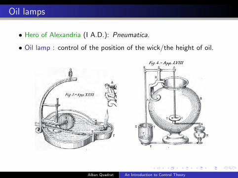
Oil lamps
• Hero of Alexandria (I A.D.): Pneumatica.
• Oil lamp : control of the position of the wick/the height of oil.
Alban Quadrat An Introduction to Control Theory
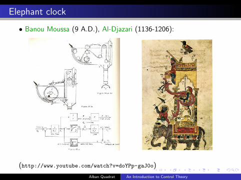
Elephant clock
• Banou Moussa (9 A.D.), Al-Djazari (1136-1206):
(http://www.youtube.com/watch?v=doYPp-gaJ0o)
Alban Quadrat An Introduction to Control Theory

Thermostat: heat control
• Cornelis Drebbel (1572-1633)
Alban Quadrat An Introduction to Control Theory
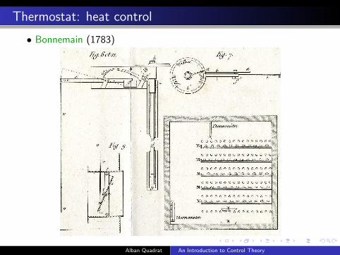
Thermostat: heat control
• Bonnemain (1783)
Alban Quadrat An Introduction to Control Theory
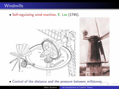
Windmills
• Self-regulating wind machine, E. Lee (1745).
• Control of the distance and the pressure between millstones, . . .
Alban Quadrat An Introduction to Control Theory

Flyball governors for windmills
• Control of the distance and the pressure between millstones
Alban Quadrat An Introduction to Control Theory

Steam engines
• Thomas Newcomen (1664-1729): pumping water out of mines.
Alban Quadrat An Introduction to Control Theory
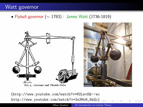
Watt governor
• Flyball governor (∼ 1783) : James Watt (1736-1819)
(http://www.youtube.com/watch?v=M2LsvSQ--wc
http://www.youtube.com/watch?v=3x3Mo6_8zGc)
Alban Quadrat An Introduction to Control Theory
Mathematical foundation of control theory
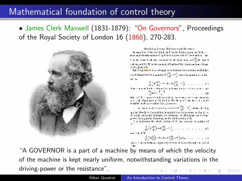
• James Clerk Maxwell (1831-1879): “On Governors”, Proceedingsof the Royal Society of London 16 (1868), 270-283.
“A GOVERNOR is a part of a machine by means of which the velocity
of the machine is kept nearly uniform, notwithstanding variations in the
driving-power or the resistance”.Alban Quadrat An Introduction to Control Theory

The first telecommunications network
• First telegraph: Samuel Morse (1791-1872), 1837, USA.
• First telegraph line between Baltimore and Washington: 1844.
• Transatlantic telegraph cable : 1866.
• The invention of the phone is patented by A. G. Bell(1847-1922) in 1876.
• First phone call using Bell’s telephone : 1878.
• First long distance phone call between Boston and Salem : 1881.
Alban Quadrat An Introduction to Control Theory

The first telecommunications network
• East coast: American Telephone & Telegraph Company (1891).
Alban Quadrat An Introduction to Control Theory
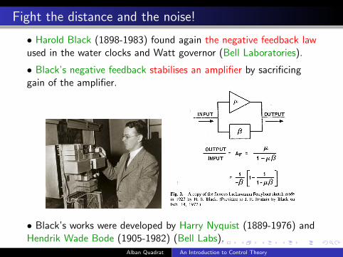
Fight the distance and the noise!
• Harold Black (1898-1983) found again the negative feedback lawused in the water clocks and Watt governor (Bell Laboratories).
• Black’s negative feedback stabilises an amplifier by sacrificinggain of the amplifier.
• Black’s works were developed by Harry Nyquist (1889-1976) andHendrik Wade Bode (1905-1982) (Bell Labs).
Alban Quadrat An Introduction to Control Theory

Rebirth of control theory
• They developed the frequency domain approach of control theory
the block diagrams and Black, Nyquist and Bode plots.
Alban Quadrat An Introduction to Control Theory
What is control theory ?
• Control theory is a branch of the mathematical systems theorywhich studies the concepts of inputs, outputs, feedback laws, . . . .
• Main goals:
Study the stability of systems.
Stabilize systems by means of feedback laws.
Track desired trajectories independently from theperturbations.
Optimize the performances of the closed-loop system.
Consider the errors of the mathematical model(robust control), . . .
(http://www.dailymotion.com/video/x2xdah_xpark-creneau-automatise-op-ii_auto)
Alban Quadrat An Introduction to Control Theory
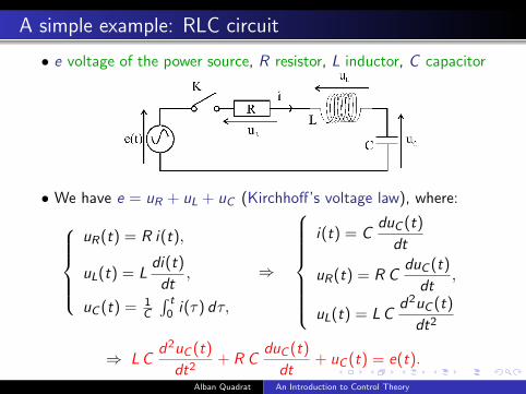
A simple example: RLC circuit
• e voltage of the power source, R resistor, L inductor, C capacitor
• We have e = uR + uL + uC (Kirchhoff’s voltage law), where:uR(t) = R i(t),
uL(t) = Ldi(t)
dt,
uC (t) = 1C
∫ t0 i(τ) dτ,
⇒
i(t) = CduC (t)
dt
uR(t) = R CduC (t)
dt,
uL(t) = L Cd2uC (t)
dt2
⇒ L Cd2uC (t)
dt2+ R C
duC (t)
dt+ uC (t) = e(t).
Alban Quadrat An Introduction to Control Theory
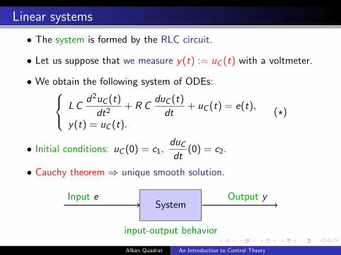
Linear systems
• The system is formed by the RLC circuit.
• Let us suppose that we measure y(t) := uC (t) with a voltmeter.
• We obtain the following system of ODEs: L Cd2uC (t)
dt2+ R C
duC (t)
dt+ uC (t) = e(t),
y(t) = uC (t).(?)
• Initial conditions: uC (0) = c1,duC
dt(0) = c2.
• Cauchy theorem ⇒ unique smooth solution.
Input eSystem
Output y
input-output behavior
Alban Quadrat An Introduction to Control Theory
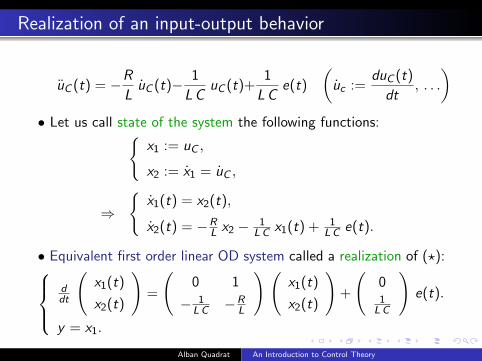
Realization of an input-output behavior
uC (t) = −R
LuC (t)− 1
L CuC (t)+
1
L Ce(t)
(uc :=
duC (t)
dt, . . .
)• Let us call state of the system the following functions:{
x1 := uC ,
x2 := x1 = uC ,
⇒
{x1(t) = x2(t),
x2(t) = −RL x2 − 1
LC x1(t) + 1LC e(t).
• Equivalent first order linear OD system called a realization of (?):ddt
(x1(t)
x2(t)
)=
(0 1
− 1LC −R
L
) (x1(t)
x2(t)
)+
(01
LC
)e(t).
y = x1.
Alban Quadrat An Introduction to Control Theory

The polynomial and state-state representations
• The state-space representation of a linear system is defined by{x(t) = A x(t) + B u(t),
y(t) = C x(t) + D u(t),
where A ∈ Rn×n, B ∈ Rn×m, C ∈ Rp×n and D ∈ Rp×m.
• The polynomial representation of a linear system is defined by
P
(d
dt
)y(t) = Q
(d
dt
)u(t),
where y := (y1 . . . yp)T , u := (u1 . . . um)T and
P ∈ Dp×p, det P 6= 0, Q ∈ Dp×m,
where D := R[
ddt
]is the commutative polynomial ring in d
dt .„e.g.,
„LC
d2
dt2+ R C
d
dt+ 1
«y(t) = e(t)
«Alban Quadrat An Introduction to Control Theory
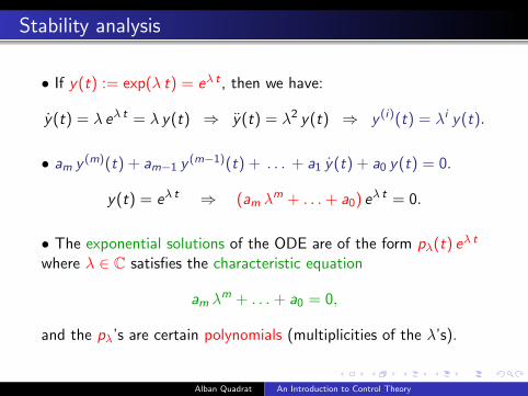
Stability analysis
• If y(t) := exp(λ t) = eλ t , then we have:
y(t) = λ eλ t = λ y(t) ⇒ y(t) = λ2 y(t) ⇒ y (i)(t) = λi y(t).
• am y (m)(t) + am−1 y (m−1)(t) + . . . + a1 y(t) + a0 y(t) = 0.
y(t) = eλ t ⇒ (am λm + . . .+ a0) eλ t = 0.
• The exponential solutions of the ODE are of the form pλ(t) eλ t
where λ ∈ C satisfies the characteristic equation
am λm + . . .+ a0 = 0,
and the pλ’s are certain polynomials (multiplicities of the λ’s).
Alban Quadrat An Introduction to Control Theory

Stability analysis
• If λ ∈ C, then λ = Re(λ) + i Im(λ) and:
eλ t = e(Re(λ)+i Im(λ)) t = eRe(λ) t e i Im(λ) t
= eRe(λ) t (cos(Im(λ) t) + i sin(Im(λ) t)).
We get: |eλ t | = eRe(λ) t .
1 If Re(λ) = 0, then |eλ t | = 1 for all t ∈ R.
2 If Re(λ) > 0, then limt→+∞ |eλ t | = +∞.
3 If Re(λ) < 0, then limt→+∞ |eλ t | = 0.
• Definition: A linear ODE with constant coefficients is said to beexponentially stable if all roots λ ∈ C of the characteristic equationlie in the left half plane C− := {s ∈ C | Re(s) < 0}.
Alban Quadrat An Introduction to Control Theory
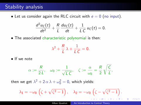
Stability analysis
• Let us consider again the RLC circuit with e = 0 (no input).
d2uC (t)
dt2+
R
L
duC (t)
dt+
1
L CuC (t) = 0.
• The associated characteristic polynomial is then:
λ2 +R
Lλ+
1
L C= 0.
• If we note
α :=R
2 L, ω0 :=
1√L C
, ζ :=α
ω0=
R
2
√C
L,
then we get λ2 + 2αλ+ ω20 = 0, which yields:
λ1 = −ω0
(ζ +
√ζ2 − 1
), λ2 = −ω0
(ζ −
√ζ2 − 1
).
Alban Quadrat An Introduction to Control Theory
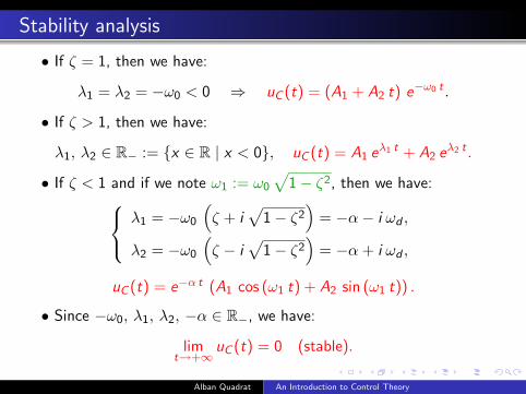
Stability analysis
• If ζ = 1, then we have:
λ1 = λ2 = −ω0 < 0 ⇒ uC (t) = (A1 + A2 t) e−ω0 t .
• If ζ > 1, then we have:
λ1, λ2 ∈ R− := {x ∈ R | x < 0}, uC (t) = A1 eλ1 t + A2 eλ2 t .
• If ζ < 1 and if we note ω1 := ω0
√1− ζ2, then we have: λ1 = −ω0
(ζ + i
√1− ζ2
)= −α− i ωd ,
λ2 = −ω0
(ζ − i
√1− ζ2
)= −α + i ωd ,
uC (t) = e−α t (A1 cos (ω1 t) + A2 sin (ω1 t)) .
• Since −ω0, λ1, λ2, −α ∈ R−, we have:
limt→+∞
uC (t) = 0 (stable).
Alban Quadrat An Introduction to Control Theory

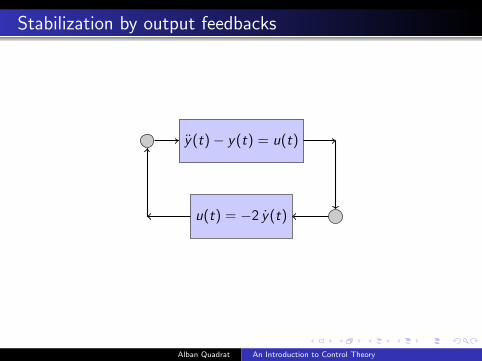
Stabilization by output feedbacks
uy(t)− y(t) = u(t)
y
• If u = 0 (no input), then the system is unstable:
y(t)− y(t) = 0 ⇒ λ2 − 1 = 0 ⇔ λ = {−1, 1}.
• Problem: Can we find a stabilizing output feedback law?
• Find a feeback law u(t) := k1 y(t) + k2 y(t) s.t. the closed-loop
y(t)− k2 y(t)− (k1 − 1) y(t) = 0 is stable.
• Example: If we take k1 = 0, k2 = −2, we get:
λ2−k2 λ−(k1−1) = 0 ⇒ λ2+2λ+1 = (λ+1)2 = 0 ⇔ λ = {−1,−1}.
Alban Quadrat An Introduction to Control Theory
Stabilization by output feedbacks
y(t)− y(t) = u(t)
u(t) = −2 y(t)
Alban Quadrat An Introduction to Control Theory
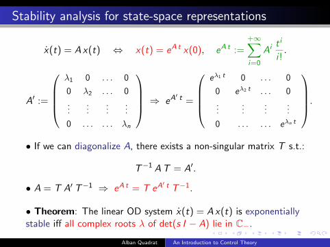
Stability analysis for state-space representations
x(t) = A x(t) ⇔ x(t) = eA t x(0), eA t :=+∞∑i=0
Ai t i
i !.
A′ :=
λ1 0 . . . 0
0 λ2 . . . 0
......
......
0 . . . . . . λn
⇒ eA′ t =
eλ1 t 0 . . . 0
0 eλ2 t . . . 0
......
......
0 . . . . . . eλn t
.• If we can diagonalize A, there exists a non-singular matrix T s.t.:
T−1 A T = A′.
• A = T A′ T−1 ⇒ eA t = T eA′ t T−1.
• Theorem: The linear OD system x(t) = A x(t) is exponentiallystable iff all complex roots λ of det(s I − A) lie in C−.
Alban Quadrat An Introduction to Control Theory

Stabilization by state feedbacks
• Let us consider the following system:
x(t) =
(−1 0
0 1
)x(t) +
(0
1
)u(t).
• We have det(s I2−A) = (s + 1)(s − 1) = 0 ⇔ s ∈ {−1, 1}.
• Problem: Can we find a stabilizing state feedback law?
• If we consider u(t) := (0 − 2) x(t), then we get:
x(t) =
((−1 0
0 1
)+
(0
1
)(0 − 2)
)x(t)
=
(−1 0
0 −1
)x(t) (stable)
Alban Quadrat An Introduction to Control Theory
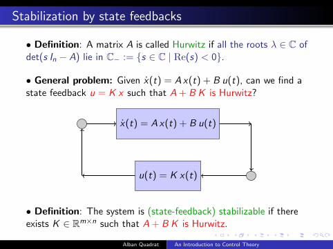
Stabilization by state feedbacks
• Definition: A matrix A is called Hurwitz if all the roots λ ∈ C ofdet(s In − A) lie in C− := {s ∈ C | Re(s) < 0}.
• General problem: Given x(t) = A x(t) + B u(t), can we find astate feedback u = K x such that A + B K is Hurwitz?
x(t) = A x(t) + B u(t)
u(t) = K x(t)
• Definition: The system is (state-feedback) stabilizable if thereexists K ∈ Rm×n such that A + B K is Hurwitz.
Alban Quadrat An Introduction to Control Theory
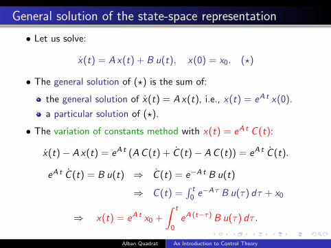
General solution of the state-space representation
• Let us solve:
x(t) = A x(t) + B u(t), x(0) = x0. (?)
• The general solution of (?) is the sum of:
the general solution of x(t) = A x(t), i.e., x(t) = eA t x(0).
a particular solution of (?).
• The variation of constants method with x(t) = eA t C (t):
x(t)− A x(t) = eA t (A C (t) + C (t)− A C (t)) = eA t C (t).
eA t C (t) = B u(t) ⇒ C (t) = e−A t B u(t)
⇒ C (t) =∫ t
0 e−A τ B u(τ) dτ + x0
⇒ x(t) = eA t x0 +
∫ t
0eA (t−τ) B u(τ) dτ .
Alban Quadrat An Introduction to Control Theory
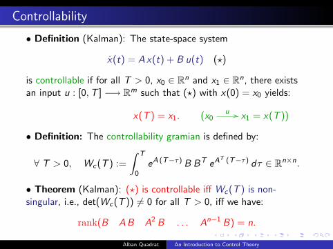
Controllability
• Definition (Kalman): The state-space system
x(t) = A x(t) + B u(t) (?)
is controllable if for all T > 0, x0 ∈ Rn and x1 ∈ Rn, there existsan input u : [0,T ] −→ Rm such that (?) with x(0) = x0 yields:
x(T ) = x1. (x0u // x1 = x(T ))
• Definition: The controllability gramian is defined by:
∀ T > 0, Wc(T ) :=
∫ T
0eA (T−τ) B BT eAT (T−τ) dτ ∈ Rn×n.
• Theorem (Kalman): (?) is controllable iff Wc(T ) is non-singular, i.e., det(Wc(T )) 6= 0 for all T > 0, iff we have:
rank(B A B A2 B . . . An−1 B) = n.
Alban Quadrat An Introduction to Control Theory
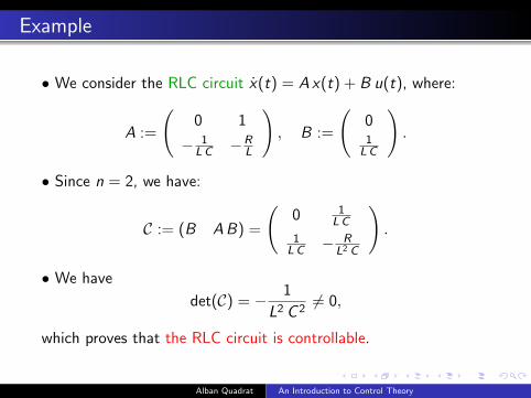
Example
• We consider the RLC circuit x(t) = A x(t) + B u(t), where:
A :=
(0 1
− 1LC −R
L
), B :=
(01
LC
).
• Since n = 2, we have:
C := (B A B) =
(0 1
LC
1LC − R
L2 C
).
• We have
det(C) = − 1
L2 C 26= 0,
which proves that the RLC circuit is controllable.
Alban Quadrat An Introduction to Control Theory
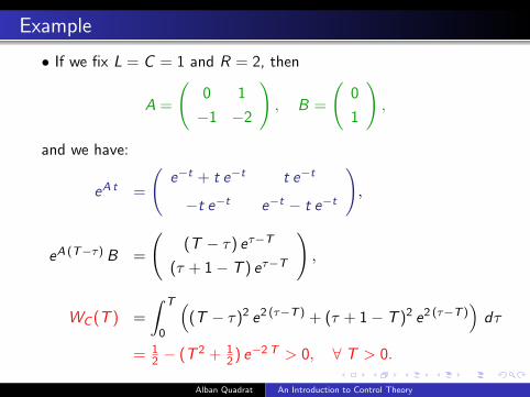
Example
• If we fix L = C = 1 and R = 2, then
A =
(0 1
−1 −2
), B =
(0
1
),
and we have:
eA t =
(e−t + t e−t t e−t
−t e−t e−t − t e−t
),
eA (T−τ) B =
((T − τ) eτ−T
(τ + 1− T ) eτ−T
),
WC (T ) =
∫ T
0
((T − τ)2 e2 (τ−T ) + (τ + 1− T )2 e2 (τ−T )
)dτ
= 12 − (T 2 + 1
2 ) e−2 T > 0, ∀ T > 0.
Alban Quadrat An Introduction to Control Theory
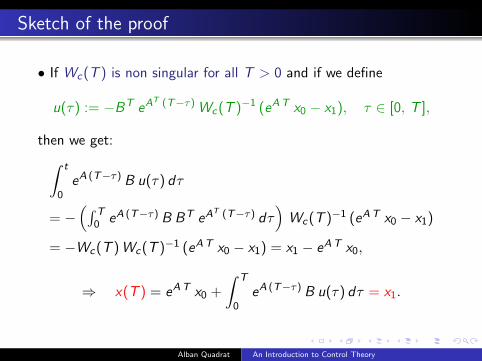
Sketch of the proof
• If Wc(T ) is non singular for all T > 0 and if we define
u(τ) := −BT eAT (T−τ) Wc(T )−1 (eAT x0 − x1), τ ∈ [0, T ],
then we get:∫ t
0eA (T−τ) B u(τ) dτ
= −(∫ T
0 eA (T−τ) B BT eAT (T−τ) dτ)
Wc(T )−1 (eAT x0 − x1)
= −Wc(T ) Wc(T )−1 (eAT x0 − x1) = x1 − eAT x0,
⇒ x(T ) = eAT x0 +
∫ T
0eA (T−τ) B u(τ) dτ = x1.
Alban Quadrat An Introduction to Control Theory
Sketch of the proof
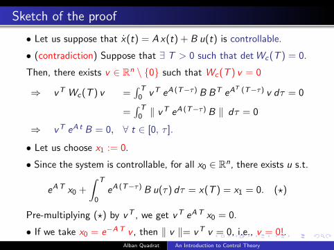
• Let us suppose that x(t) = A x(t) + B u(t) is controllable.
• (contradiction) Suppose that ∃ T > 0 such that det Wc(T ) = 0.
Then, there exists v ∈ Rn \ {0} such that Wc(T ) v = 0
⇒ vT Wc(T ) v =∫ T
0 vT eA (T−τ) B BT eAT (T−τ) v dτ = 0
=∫ T
0 ‖ vT eA (T−τ) B ‖ dτ = 0
⇒ vT eA t B = 0, ∀ t ∈ [0, τ ].
• Let us choose x1 := 0.
• Since the system is controllable, for all x0 ∈ Rn, there exists u s.t.
eAT x0 +
∫ T
0eA (T−τ) B u(τ) dτ = x(T ) = x1 = 0. (?)
Pre-multiplying (?) by vT , we get vT eAT x0 = 0.
• If we take x0 = e−AT v , then ‖ v ‖= vT v = 0, i.e., v = 0!.Alban Quadrat An Introduction to Control Theory
Sketch of the proof
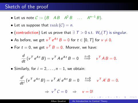
• Let us note C := (B A B A2 B . . . An−1 B).
• Let us suppose that rank (C) = n.
• (contradiction) Let us prove that ∃ T > 0 s.t. Wc(T ) is singular.
• As before, we get vT eA t B = 0 for t ∈ [0,T ] for v 6= 0.
• For t = 0, we get vT B = 0. Morever, we have:
d
dt(vT eA t B) = vT A eA t B = 0
t=0=⇒ vT A B = 0.
• Similarly, for i = 2, . . . , n − 1, we obtain:
d i
dt i(vT eA t B) = vT Ai eA t B = 0
t=0=⇒ vT Ai B = 0.
⇒ vT C = 0 ⇒ v = 0!
Alban Quadrat An Introduction to Control Theory
Sketch of the proof
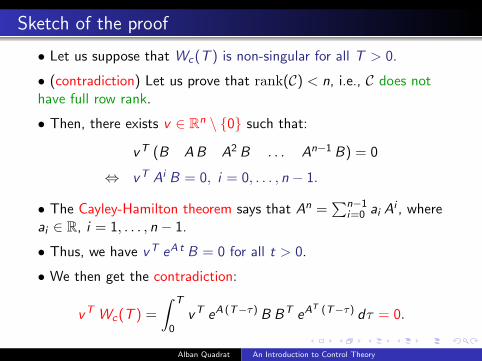
• Let us suppose that Wc(T ) is non-singular for all T > 0.
• (contradiction) Let us prove that rank(C) < n, i.e., C does nothave full row rank.
• Then, there exists v ∈ Rn \ {0} such that:
vT (B A B A2 B . . . An−1 B) = 0
⇔ vT Ai B = 0, i = 0, . . . , n − 1.
• The Cayley-Hamilton theorem says that An =∑n−1
i=0 ai Ai , whereai ∈ R, i = 1, . . . , n − 1.
• Thus, we have vT eA t B = 0 for all t > 0.
• We then get the contradiction:
vT Wc(T ) =
∫ T
0vT eA (T−τ) B BT eAT (T−τ) dτ = 0.
Alban Quadrat An Introduction to Control Theory

Observability
• Definition (Kalman): The state-space representation{x(t) = A x(t) + B u(t),
y(t) = C x(t) + D u(t),(?)
is observable if for any T > 0, then the initial conditionx(0) = x0 ∈ Rn can be determined from the history of the input uand the output y in the interval [0, T ].
• Definition: The observability gramian is defined by:
∀ T > 0, Wo(T ) :=
∫ T
0eAT (T−τ) CT C eAT (T−τ) dτ ∈ Rn×n.
• Theorem: (?) is observable iff Wo(T ) is non-singular ∀ T > 0
⇔ rank (O) = n, O :=
C
C A...
C An−1
.Alban Quadrat An Introduction to Control Theory
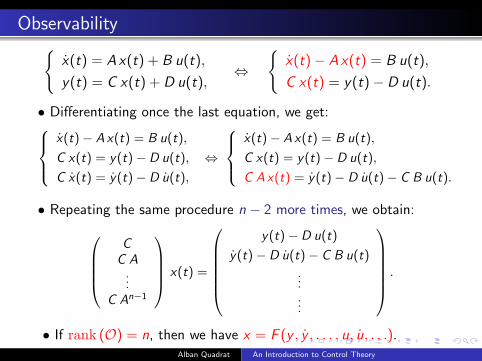
Observability{x(t) = A x(t) + B u(t),
y(t) = C x(t) + D u(t),⇔
{x(t)− A x(t) = B u(t),
C x(t) = y(t)− D u(t).
• Differentiating once the last equation, we get:x(t)− A x(t) = B u(t),
C x(t) = y(t)− D u(t),
C x(t) = y(t)− D u(t),
⇔
x(t)− A x(t) = B u(t),
C x(t) = y(t)− D u(t),
C A x(t) = y(t)− D u(t)− C B u(t).
• Repeating the same procedure n − 2 more times, we obtain:C
C A...
C An−1
x(t) =
y(t)− D u(t)
y(t)− D u(t)− C B u(t)
...
...
.
• If rank (O) = n, then we have x = F (y , y , . . . , u, u, . . .).Alban Quadrat An Introduction to Control Theory
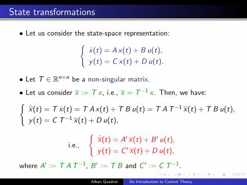
State transformations
• Let us consider the state-space representation:{x(t) = A x(t) + B u(t),
y(t) = C x(t) + D u(t).
• Let T ∈ Rn×n be a non-singular matrix.
• Let us consider x := T x , i.e., x = T−1 x . Then, we have:{x(t) = T x(t) = T A x(t) + T B u(t) = T A T−1 x(t) + T B u(t),
y(t) = C T−1 x(t) + D u(t),
i.e.,
{x(t) = A′ x(t) + B ′ u(t),
y(t) = C ′ x(t) + D u(t),
where A′ := T A T−1, B ′ := T B and C ′ := C T−1.
Alban Quadrat An Introduction to Control Theory
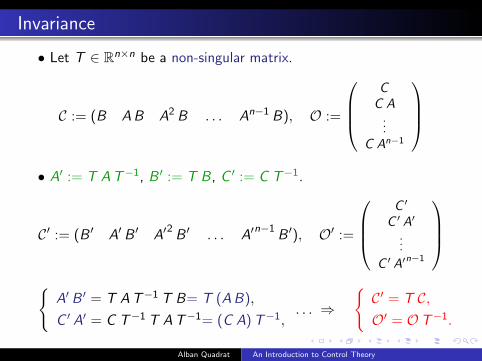
Invariance
• Let T ∈ Rn×n be a non-singular matrix.
C := (B A B A2 B . . . An−1 B), O :=
C
C A...
C An−1
• A′ := T A T−1, B ′ := T B, C ′ := C T−1.
C′ := (B ′ A′ B ′ A′2
B ′ . . . A′n−1
B ′), O′ :=
C ′
C ′ A′
...
C ′ A′n−1
{
A′ B ′ = T A T−1 T B= T (A B),
C ′ A′ = C T−1 T A T−1= (C A) T−1,. . . ⇒
{C′ = T C,O′ = OT−1.
Alban Quadrat An Introduction to Control Theory

Canonical decomposition
• Theorem (Kalman): Let rank (C) = k < n. Then, there exists anon-singular matrix T ∈ Rn×n such that the equivalent system x(t) = A′ x(t) + B ′ u(t), x =
(x1
x2
):= T x ,
y(t) = C ′ x(t) + D u(t), x1 ∈ Rk , x2 ∈ Rn−k ,
is such that
A′ := T A T−1 =
(A11 A12
0 A22
), B ′ := T B =
(B1
0
),
where A11 ∈ Rk×k , A12 ∈ Rk×(n−k), A22 ∈ R(n−k)×(n−k) and:
x1 = A11 x1 + B1 u is controllable.
Alban Quadrat An Introduction to Control Theory
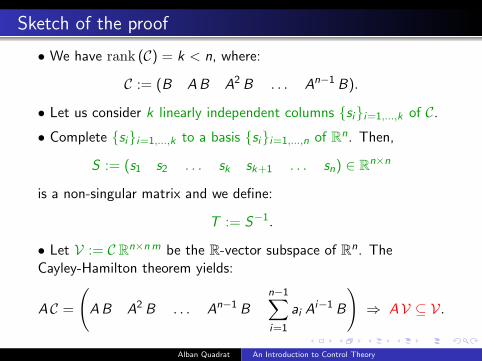
Sketch of the proof
• We have rank (C) = k < n, where:
C := (B A B A2 B . . . An−1 B).
• Let us consider k linearly independent columns {si}i=1,...,k of C.
• Complete {si}i=1,...,k to a basis {si}i=1,...,n of Rn. Then,
S := (s1 s2 . . . sk sk+1 . . . sn) ∈ Rn×n
is a non-singular matrix and we define:
T := S−1.
• Let V := C Rn×n m be the R-vector subspace of Rn. TheCayley-Hamilton theorem yields:
A C =
(A B A2 B . . . An−1 B
n−1∑i=1
ai Ai−1 B
)⇒ AV ⊆ V.
Alban Quadrat An Introduction to Control Theory
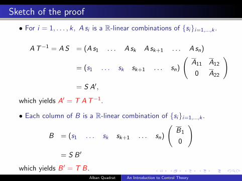
Sketch of the proof
• For i = 1, . . . , k , A si is a R-linear combinations of {si}i=1,...,k .
A T−1 = A S = (A s1 . . . A sk A sk+1 . . . A sn)
= (s1 . . . sk sk+1 . . . sn)
(A11 A12
0 A22
)= S A′,
which yields A′ = T A T−1.
• Each column of B is a R-linear combination of {si}i=1,...,k .
B = (s1 . . . sk sk+1 . . . sn)
(B1
0
)= S B ′
which yields B ′ = T B.Alban Quadrat An Introduction to Control Theory
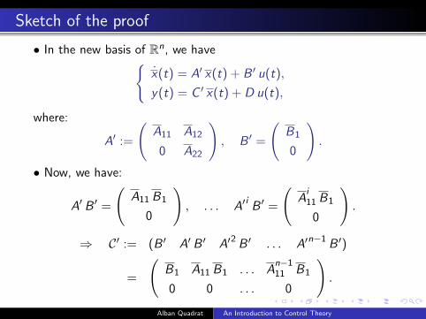
Sketch of the proof
• In the new basis of Rn, we have{x(t) = A′ x(t) + B ′ u(t),
y(t) = C ′ x(t) + D u(t),
where:
A′ :=
(A11 A12
0 A22
), B ′ =
(B1
0
).
• Now, we have:
A′ B ′ =
(A11 B1
0
), . . . A′
iB ′ =
(A
i11 B1
0
).
⇒ C′ := (B ′ A′ B ′ A′2 B ′ . . . A′n−1 B ′)
=
(B1 A11 B1 . . . A
n−111 B1
0 0 . . . 0
).
Alban Quadrat An Introduction to Control Theory
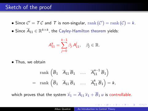
Sketch of the proof
• Since C′ = T C and T is non-singular, rank (C′) = rank (C) = k .
• Since A11 ∈ Rk×k , the Cayley-Hamilton theorem yields:
Ak11 =
k−1∑j=0
βj Aj11, βj ∈ R.
• Thus, we obtain
rank(
B1 A11 B1 . . . An−111 B1
)= rank
(B1 A11 B1 . . . A
k11 B1
)= k,
which proves that the system x1 = A11 x1 + B1 u is controllable.
Alban Quadrat An Introduction to Control Theory
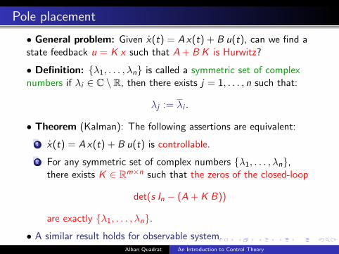
Pole placement
• General problem: Given x(t) = A x(t) + B u(t), can we find astate feedback u = K x such that A + B K is Hurwitz?
• Definition: {λ1, . . . , λn} is called a symmetric set of complexnumbers if λi ∈ C \ R, then there exists j = 1, . . . , n such that:
λj := λi .
• Theorem (Kalman): The following assertions are equivalent:
1 x(t) = A x(t) + B u(t) is controllable.
2 For any symmetric set of complex numbers {λ1, . . . , λn},there exists K ∈ Rm×n such that the zeros of the closed-loop
det(s In − (A + K B))
are exactly {λ1, . . . , λn}.
• A similar result holds for observable system.Alban Quadrat An Introduction to Control Theory

Stabilizability
• Definition: The system x(t) = A x(t) + B u(t) is state-feedbackstabilizable if there exists K ∈ Rm×n such that A + B K is Hurwitz.
• Corollary: A controllable system is stabilizable.
• If T ∈ Rn×n is non-singular and x = T x , then
x(t) = A x(t) + B u(t) ⇔ x(t) = A′ x(t) + B ′ u(t)
A′ :=
(A11 A12
0 A22
), B ′ =
(B1
0
),
where x1 = A11 x1 + B1 u is controllable, x2 = A22 x2 no inputs!
• det(s In − A′) = det(s Ik − A11) det(s In−k − A22).
• Corollary: The system x(t) = A x(t) + B u(t) is state-feedbackstabilizable iff A22 is Hurwitz.
Alban Quadrat An Introduction to Control Theory
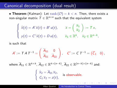
Canonical decomposition (dual result)
• Theorem (Kalman): Let rank (O) = k < n. Then, there exists anon-singular matrix T ∈ Rn×n such that the equivalent system x(t) = A′ x(t) + B ′ u(t), x =
(x1
x2
):= T x ,
y(t) = C ′ x(t) + D u(t), x1 ∈ Rk , x2 ∈ Rn−k ,
is such that
A′ := T A T−1 =
(A11 0
A21 A22
), C ′ := C T−1 =
(C 1 0
),
where A11 ∈ Rk×k , A12 ∈ Rk×(n−k), A22 ∈ R(n−k)×(n−k) and:{x2 = A21 x2,
C1 x2 = z(t),is observable.
Alban Quadrat An Introduction to Control Theory
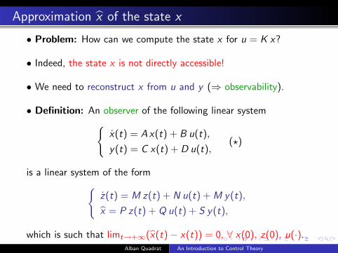
Approximation x of the state x
• Problem: How can we compute the state x for u = K x?
• Indeed, the state x is not directly accessible!
• We need to reconstruct x from u and y (⇒ observability).
• Definition: An observer of the following linear system{x(t) = A x(t) + B u(t),
y(t) = C x(t) + D u(t),(?)
is a linear system of the form{z(t) = M z(t) + N u(t) + M y(t),
x = P z(t) + Q u(t) + S y(t),
which is such that limt→+∞(x(t)− x(t)) = 0, ∀ x(0), z(0), u(·).Alban Quadrat An Introduction to Control Theory
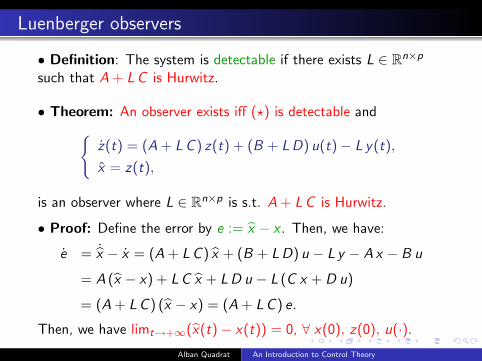
Luenberger observers
• Definition: The system is detectable if there exists L ∈ Rn×p
such that A + L C is Hurwitz.
• Theorem: An observer exists iff (?) is detectable and{z(t) = (A + L C ) z(t) + (B + L D) u(t)− L y(t),
x = z(t),
is an observer where L ∈ Rn×p is s.t. A + L C is Hurwitz.
• Proof: Define the error by e := x − x . Then, we have:
e = ˙x − x = (A + L C ) x + (B + L D) u − L y − A x − B u
= A (x − x) + L C x + L D u − L (C x + D u)
= (A + L C ) (x − x) = (A + L C ) e.
Then, we have limt→+∞(x(t)− x(t)) = 0, ∀ x(0), z(0), u(·).
Alban Quadrat An Introduction to Control Theory

Polynomial systems
• Let R[
ddt
]be a commutative polynomial ring in d
dt .
P :=n∑
i=0
aid
dt
i
∈ D, ai ∈ R,d
dt
i
=d
dt◦ . . . ◦ d
dt=
d i
dt i.
• The polynomial representation of a linear system is defined by
P
(d
dt
)y(t) = Q
(d
dt
)u(t),
where y := (y1 . . . yp)T , u := (u1 . . . um)T and:
P ∈ Dp×p, det P 6= 0, Q ∈ Dp×m.
• Example: P(
ddt
):= d
dt In − A, Q(
ddt
):= B u.
• Problem: Extension of the concept of controllability(no states!)?
Alban Quadrat An Introduction to Control Theory
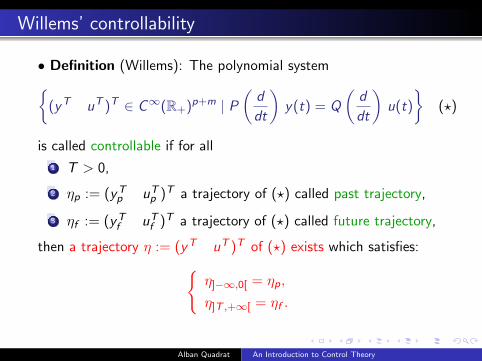
Willems’ controllability
• Definition (Willems): The polynomial system{(yT uT )T ∈ C∞(R+)p+m | P
(d
dt
)y(t) = Q
(d
dt
)u(t)
}(?)
is called controllable if for all
1 T > 0,
2 ηp := (yTp uT
p )T a trajectory of (?) called past trajectory,
3 ηf := (yTf uT
f )T a trajectory of (?) called future trajectory,
then a trajectory η := (yT uT )T of (?) exists which satisfies:{η]−∞,0[ = ηp,
η]T ,+∞[ = ηf .
Alban Quadrat An Introduction to Control Theory

Willems’ controllability
Alban Quadrat An Introduction to Control Theory
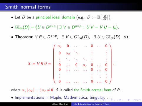
Smith normal forms
• Let D be a principal ideal domain (e.g., D := R[
ddt
]).
• GLp(D) = {U ∈ Dp×p | ∃ V ∈ Dp×p : U V = V U = Ip}.
• Theorem: ∀ R ∈ Dq×p, ∃ V ∈ GLq(D), ∃ U ∈ GLp(D) s.t.
S := V R U =
α1 0 . . . . . . 0 . . . 0
0 α2. . .
......
.... . .
. . .. . .
......
0 . . . 0 αr 0 . . . 00 . . . . . . . . . 0 . . . 0...
.... . .
...0 . . . . . . . . . 0 . . . 0
,
where α1 |α2 | . . . |αr 6= 0. S is called the Smith normal form of R.
• Implementations in Maple, Mathematica, Singular, . . .
Alban Quadrat An Introduction to Control Theory
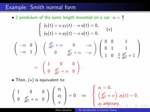
Example: Smith normal form
• 2 pendulum of the same length mounted on a car: α = gl{
y1(t) + α y1(t)− α u(t) = 0,
y2(t) + α y2(t)− α u(t) = 0,(?)
(−α 0
−α 1
) (d2
dt2 + α 0 −α0 d2
dt2 + α −α
) 0 0 1
0 1 1
1 0 1α
d2
dt2 + 1
=
(1 0 0
0 d2
dt2 + α 0
).
• Then, (?) is equivalent to:(1 0 0
0 d2
dt2 + α 0
) z1
z2
v
= 0 ⇔
z1 = 0,(
d2
dt2 + α)
z2(t) = 0,
z3 arbitrary.
Alban Quadrat An Introduction to Control Theory
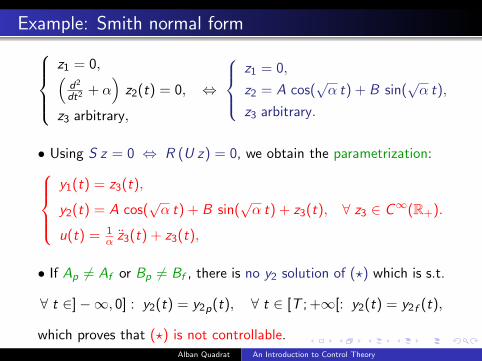
Example: Smith normal formz1 = 0,(
d2
dt2 + α)
z2(t) = 0,
z3 arbitrary,
⇔
z1 = 0,
z2 = A cos(√α t) + B sin(
√α t),
z3 arbitrary.
• Using S z = 0 ⇔ R (U z) = 0, we obtain the parametrization:y1(t) = z3(t),
y2(t) = A cos(√α t) + B sin(
√α t) + z3(t),
u(t) = 1α z3(t) + z3(t),
∀ z3 ∈ C∞(R+).
• If Ap 6= Af or Bp 6= Bf , there is no y2 solution of (?) which is s.t.
∀ t ∈]−∞, 0] : y2(t) = y2p(t), ∀ t ∈ [T ; +∞[: y2(t) = y2f (t),
which proves that (?) is not controllable.Alban Quadrat An Introduction to Control Theory

Willems’ controllability
• Theorem: The polynomial system{(yT uT )T ∈ C∞(R+)p+m | P
(d
dt
)y(t) = Q
(d
dt
)u(t)
}is controllable iff the Smith normal form of the matrix
R :=
(P
(d
dt
)− Q
(d
dt
))∈ Dp×(p+m)
is equal to S = (Ip 0), i.e., α1 = . . . = αp = 1.
• Let U := (U1 U2), W := U−1 = (W T1 W T
2 )T . Then, we get:
R = V−1 (Ip 0) U−1 ⇔(
RW2
)(U1 V−1 U2) = Ip+m.
• If T := U1 V−1 and Π := T R, then Π2 = T (R T ) R = Π.
Parametrization: R
(yu
)= 0 ⇔
(yu
)= U2 ξ, ∀ ξ ∈ C∞(R+)m.
Alban Quadrat An Introduction to Control Theory
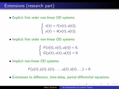
Extensions (research part)
• Explicit first order non-linear OD systems:{x(t) = f (x(t), u(t)),
y(t) = h(x(t), u(t)).
• Implicit first order non-linear OD systems:{F (x(t), x(t), u(t)) = 0,
G (y(t), x(t), u(t)) = 0.
• Implicit non-linear OD systems:
F (y(t), y(t), y(t), . . . , u(t), u(t), . . .) = 0.
• Extensions to difference, time-delay, partial differential equations.
Alban Quadrat An Introduction to Control Theory
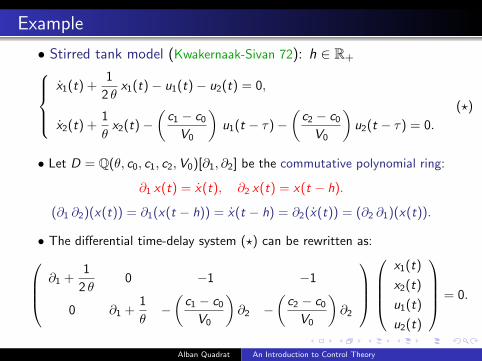
Example
• Stirred tank model (Kwakernaak-Sivan 72): h ∈ R+x1(t) +
1
2 θx1(t)− u1(t)− u2(t) = 0,
x2(t) +1
θx2(t)−
(c1 − c0
V0
)u1(t − τ)−
(c2 − c0
V0
)u2(t − τ) = 0.
(?)
• Let D = Q(θ, c0, c1, c2,V0)[∂1, ∂2] be the commutative polynomial ring:
∂1 x(t) = x(t), ∂2 x(t) = x(t − h).
(∂1 ∂2)(x(t)) = ∂1(x(t − h)) = x(t − h) = ∂2(x(t)) = (∂2 ∂1)(x(t)).
• The differential time-delay system (?) can be rewritten as: ∂1 +1
2 θ0 −1 −1
0 ∂1 +1
θ−(
c1 − c0
V0
)∂2 −
(c2 − c0
V0
)∂2
x1(t)
x2(t)
u1(t)
u2(t)
= 0.
Alban Quadrat An Introduction to Control Theory

Example
• Linearization of the Navier-Stokes ∼ a parabolic Poiseuille profile∂t u1 + 4 y (1− y) ∂x u1 − 4 (2 y − 1) u2 − ν (∂2
x + ∂2y ) u1 + ∂x p = 0,
∂t u2 + 4 y (1− y) ∂x u2 − ν (∂2x + ∂2
y ) u2 + ∂y p = 0,
∂x u1 + ∂y u2 = 0.
• Let D = Q(ν)〈∂t , ∂x , ∂y , y〉 be the associative algebra defined by
∂t ∂x = ∂x ∂t , ∂t y = y ∂t , ∂t ∂y = ∂y ∂t , ∂x ∂y = ∂y ∂x , ∂x y = y ∂x ,
∂y y = y ∂y + 1 (∂y (y f (y)) = y ∂y f (y) + f (y)).
• The PD linear system can be rewritten as:(∂t + 4 y (1− y) ∂x − ν (∂2
x + ∂2y ) −4 (2 y − 1) ∂x
0 ∂t + 4 y (1− y) ∂x − ν (∂2x + ∂2
y ) ∂y
∂x ∂y 0
) (u1(x1, x2, t)
u2(x1, x2, t)
p(x1, x2, t)
)= 0.
Alban Quadrat An Introduction to Control Theory

Finitely presented modules
• Let D be a noetherian domain, R ∈ Dq×p.
• We consider the left D-homomorphism (i.e., left D-linear map):
D1×q .R−→ D1×p
λ = (λ1 . . . λq) 7−→ λR.
• We introduce the finitely presented left D-module:
M := cokerD(.R) = D1×p/(D1×q R).
• M = D1×p/(D1×q R) is formed by the classes π(λ) of λ ∈ D1×p:
π(λ) = π(λ′) ⇔ ∃ µ ∈ D1×q : λ = λ′ + µR.
• M is a left D-module: ∀ λ, λ′ ∈ D1×p, ∀ d ∈ D:
π(λ) + π(λ′) := π(λ+ λ′), d π(λ) := π(d λ).
Alban Quadrat An Introduction to Control Theory
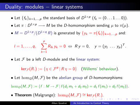
Duality: modules − linear systems
• Let {fk}k=1,...,p the standard basis of D1×p (fk = (0 . . . 1 . . . 0)).
• Let π : D1×p −→ M be the D-homomorphism sending µ to π(µ).
• M = D1×p/(D1×q R) is generated by {yk = π(fk)}k=1,...,p and:
l = 1, . . . , q,
p∑k=1
Rlk yk = 0 ⇔ R y = 0, y = (y1 . . . yp)T .
• Let F be a left D-module and the linear system:
kerF (R.) := {η ∈ Fp |R η = 0} (Willems’ behaviour).
• Let homD(M,F) be the abelian group of D-homomorphisms:
homD(M,F) := {f : M → F | f (d1 m1 + d2 m2) = d1 f (m1) + d2 f (m2)}.
• Theorem (Malgrange): homD(M,F) ∼= kerF (R.).
Alban Quadrat An Introduction to Control Theory

Module theory
• Definition: 1. M is free if ∃ r ∈ Z+ such that M ∼= D1×r .
2. M is stably free if ∃ r , s ∈ Z+ such that M ⊕ D1×s ∼= D1×r .
3. M is projective if ∃ r ∈ Z+ and a D-module P such that:
M ⊕ P ∼= D1×r .
4. M is reflexive if ε : M −→ homD(homD(M,D),D) is anisomorphism, where:
ε(m)(f ) = f (m), ∀ m ∈ M, f ∈ homD(M,D).
5. M is torsion-free if:
t(M) = {m ∈ M | ∃ 0 6= d ∈ D : d m = 0} = 0.
6. M is torsion if t(M) = M.
Alban Quadrat An Introduction to Control Theory

Classification of modules
• Theorem: 1. We have the following implications:
free⇒ stably free⇒ projective⇒ reflexive⇒ torsion-free.
2. If D is a principal domain (e.g., B1(Q) := Q(t)〈∂〉), then:
torsion-free = free.
3. If D is a hereditary ring (e.g., A1(Q) := Q[t]〈∂〉), then:
torsion-free = projective.
4. If D = k[∂1, . . . , ∂n] and k a field, then:
projective = free (Quillen-Suslin theorem).
4. If D = An(k) or Bn(k), k is a field of characteristic 0, then
projective = free (Stafford theorem),
for modules of rank at least 2.Alban Quadrat An Introduction to Control Theory
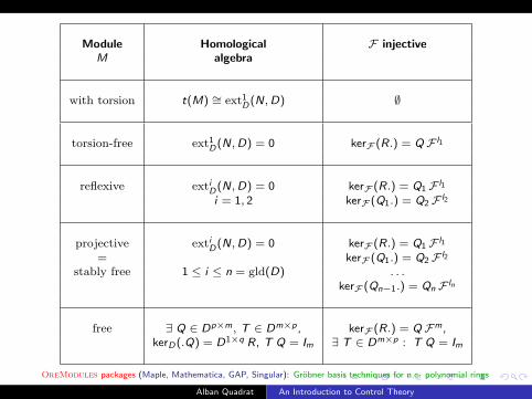
Module Homological F injectiveM algebra
with torsion t(M) ∼= ext1D(N,D) ∅
torsion-free ext1D(N,D) = 0 kerF (R.) = Q F l1
reflexive extiD(N,D) = 0 kerF (R.) = Q1 F l1
i = 1, 2 kerF (Q1.) = Q2 F l2
projective extiD(N,D) = 0 kerF (R.) = Q1 F l1
= kerF (Q1.) = Q2 F l2
stably free 1 ≤ i ≤ n = gld(D) . . .kerF (Qn−1.) = Qn F ln
free ∃ Q ∈ Dp×m, T ∈ Dm×p , kerF (R.) = Q Fm,kerD(.Q) = D1×q R, T Q = Im ∃ T ∈ Dm×p : T Q = Im
OreModules packages (Maple, Mathematica, GAP, Singular): Grobner basis techniques for n.c. polynomial rings
Alban Quadrat An Introduction to Control Theory
Homological algebra techniques
• K := Q(D) the left and right quotient field of D.
• N := Dq×1/(R Dp×1) the transpose of M = D1×p/(D1×q R).
t(M) := {m ∈ M | ∃ d ∈ D\{0} : d m = 0} ∼= torD1 (K/D,M) ∼= ext1D(N,D).
Alban Quadrat An Introduction to Control Theory
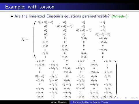
Example: with torsion
• Are the linearized Einstein’s equations parametrizable? (Wheeler)
R =
∂22 + ∂2
3 − ∂2t ∂2
1 ∂21 −∂2
1
∂22 ∂2
1 + ∂23 − ∂
2t ∂2
2 −∂22
∂23 ∂2
3 ∂21 + ∂2
2 − ∂2t −∂2
3
∂2t ∂2
t ∂2t ∂2
1 + ∂22 + ∂3
3
0 0 ∂1 ∂2 −∂1 ∂2
∂2 ∂3 0 0 −∂2 ∂3
∂3 ∂t ∂3 ∂t 0 0
0 ∂1 ∂3 0 −∂1 ∂3
∂2 ∂t 0 ∂2 ∂t 0
0 ∂1 ∂t ∂1 ∂t 0
−2 ∂1 ∂2 0 0 −2 ∂1 ∂3 0 2 ∂1 ∂t
−2 ∂1 ∂2 −2 ∂2 ∂3 0 0 2 ∂2 ∂t 0
0 −2 ∂2 ∂3 2 ∂3 ∂t −2 ∂1 ∂3 0 0
0 0 −2 ∂3 ∂t 0 −2 ∂2 ∂t −2 ∂1 ∂t
∂32 − ∂
2t −∂1 ∂3 0 −∂2 ∂3 ∂1 ∂t ∂2 ∂t
−∂1 ∂3 ∂21 − ∂
2t ∂2 ∂t −∂1 ∂2 ∂3 ∂t 0
0 −∂2 ∂t ∂21 + ∂2
2 −∂1 ∂t −∂2 ∂3 −∂1 ∂3
−∂2 ∂3 −∂1 ∂2 ∂1 ∂t ∂22 − ∂
2t 0 ∂3 ∂t
−∂1 ∂t −∂3 ∂t −∂2 ∂3 0 ∂21 + ∂2
3 −∂1 ∂3
−∂2 ∂t 0 −∂1 ∂3 −∂3 ∂t −∂1 ∂3 ∂22 + ∂2
3
Alban Quadrat An Introduction to Control Theory

Example: torsion-free and reflexive modules
• Wind tunnel model (Manitius 84): torsion-free but not reflexivex1(t) + a x1(t)− k a x2(t − h) = 0,
x2(t)− x3(t) = 0,
x3(t) + ω2 x2(t) + 2 ζ ω x3(t)− ω2 u(t) = 0,
⇔
x1(t) = ω2 k a z(t − h),
x2(t) = ω2 z(t)− aω2 z(t), (motion planning
x3(t) = ω2 z(t) + ω2 a z(t), (Mounier et al 95))
u(t) = z(t)(3) + (2 ζ ω + a) z(t) + (ω2 + 2 aω ζ) z(t) + aω z(t).
• First group of Maxwell equations: reflexive but not projective∂~B
∂t+ ~∇∧ ~E = ~0,
~∇. ~B = 0,
⇔
~E = −∂~A
∂t− ~∇V ,
~B = ~∇∧ ~A. −∂~A
∂t− ~∇V = ~0,
~∇∧ ~A = ~0,
⇔
~A = ~∇ ξ,
V = −∂ξ∂t.
(gauge)
Alban Quadrat An Introduction to Control Theory
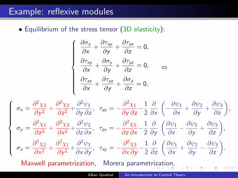
Example: reflexive modules
• Equilibrium of the stress tensor (3D elasticity):
∂σx
∂x+∂τxy∂y
+∂τzx∂z
= 0,
∂τxy∂x
+∂σy
∂y+∂τyz∂z
= 0,
∂τzx∂x
+∂τyz∂y
+∂σz
∂z= 0,
⇔
σx =∂2χ3
∂y 2+∂2χ2
∂z2+∂2ψ1
∂y ∂z, τyz = − ∂2χ1
∂y ∂z−1
2
∂
∂x
(−∂ψ1
∂x+∂ψ2
∂y+∂ψ3
∂z
),
σy =∂2χ1
∂z2+∂2χ3
∂x2+∂2ψ2
∂z ∂x, τzx = − ∂2χ2
∂z ∂x−1
2
∂
∂y
(∂ψ1
∂x− ∂ψ2
∂y+∂ψ3
∂z
),
σz =∂2χ2
∂x2+∂2χ1
∂y 2+∂2ψ3
∂x ∂y, τxy = − ∂2χ3
∂x ∂y−1
2
∂
∂z
(∂ψ1
∂x+∂ψ2
∂y− ∂ψ3
∂z
).
Maxwell parametrization, Morera parametrization.
Alban Quadrat An Introduction to Control Theory

Constructive version of Stafford’s theorem
• The time-varying linear control system{x1(t)− t u1(t) = 0,
x2(t)− u2(t) = 0,
is injectively parametrized by (Stafford (Robertz, Q.))x1(t) = t2 ξ1(t)− t ξ2(t) + ξ2(t),
x2(t) = t (t + 1) ξ1(t)− (t + 1) ξ2(t) + ξ2(t),
u1(t) = t ξ1(t) + 2 ξ1(t)− ξ2(t),
u2(t) = t (t + 1) ξ1(t) + (2 t + 1) ξ1(t)− (t + 1) ξ2(t),
and {ξ1, ξ2} is a basis of the free left A1(Q)-module M as:{ξ1(t) = (t + 1) u1(t)− u2(t),
ξ2(t) = (t + 1) x1(t)− t x2(t).
• Idem for ∂1 y1 + ∂2 y2 + ∂3 y3 + x3 y1 = 0.Alban Quadrat An Introduction to Control Theory

Standard textbooks in control theory
• R. E. Kalman, P. L. Falb, M. A. Arbib, Topics in MathematicalSystem Theory, McGraw-Hill, 1969.
• R. Brockett, Finite Dimensional Linear Systems, Wiley, 1970.
• T. Kailath, Linear Systems, Prentice-Hall, 1980.
• J. W. Polderman, J. C. Willems, Introduction to MathematicalSystems Theory. A Behavioral Approach, Texts in Mathematics 26,Springer, 1998.
• V. Kucera, Discrete Linear Control: The Polynomial EquationApproach, Wiley, Chichester 1979.
• J. C. Doyle, B. A. Francis, A. R. Tannenbaum, Feedback ControlTheory, Macmillan, 1992.
Alban Quadrat An Introduction to Control Theory
References (research part)
• M. Auslander, M. Bridger, Stable Module Theory, Memoirs ofthe American Mathematical Society, 94 American MathematicalSociety, 1969.
• T. Becker, V. Weispfenning, Grobner Bases. A ComputationalApproach to Commutative Algebra, Springer, NewYork, 1993.
• J. E. Bjork, Rings of Differential Operators, North Holland, 1979.
• H. Cartan, S. Eilenberg, Homological Algebra, PrincetonUniversity Press, 1956.
• F. Chyzak, A. Quadrat, D. Robertz, “Effective algorithms forparametrizing linear control systems over Ore algebras”, Appl.Algebra Engrg. Comm. Comput., 16 (2005), 319-376.
Alban Quadrat An Introduction to Control Theory

References (research part)
• F. Chyzak, A. Quadrat, D. Robertz, “OreModules: Asymbolic package for the study of multidimensional linearsystems”, in Applications of Time-Delay Systems, J. Chiasson andJ.-J. Loiseau (eds.), Lecture Notes in Control and Inform. 352,Springer, 2007, 233–264, OreModules project:http://wwwb.math.rwth-aachen.de/OreModules.
• M. Fliess, H. Mounier, “Controllability and observability of lineardelay systems: an algebraic approach”, ESAIM Control Optim.Calc. Var., 3 (1998), 301-314.
• M. Kashiwara, Algebraic Study of Systems of Partial DifferentialEquations, Master Thesis, Tokyo Univ. 1970, Memoires de laSociete Mathematiques de France 63 (1995) (English translation).
• T. Y. Lam, Lectures on Modules and Rings, Graduate Texts inMathematics 189, Springer, 1999.
Alban Quadrat An Introduction to Control Theory
References (research part)
• J. C. McConnell, J. C. Robson, Noncommutative NoetherianRings, American Mathematical Society, 2000.
• J.-F. Pommaret, A. Quadrat, “Algebraic analysis of linearmultidimensional control systems”, IMA J. Math. Control Inform.,16 (1999), 275-297.
• A. Quadrat, “An introduction to constructive algebraic analysisand its applications”, Les cours du CIRM, 1 no. 2: JourneesNationales de Calcul Formel (2010), 281–471(http://hal.archives-ouvertes.fr/inria-00506104/fr/).
• J. Wood, “Modules and behaviours in nD systems theory”,Multidimens. Syst. Signal Process., 11 (2000), 11-48.
Alban Quadrat An Introduction to Control Theory