ARCH STRUCTURE

CHAPTER 4

AN INTRODUCTION OF THE FINITE ELEMENT METHOD

4-1 Definition:

The finite element method is a tool to solve one dimensional, two –

dimensional and three – dimensional structures with approximation

instead of solving complicated partial differential equations. The

structure is discredited into a set of elements joined together at some

points called nodes or nodal points. These nodes are similar to the

joints in the one – dimensional structures which were investigated in

the previous chapters. The nodes could be the common corners

between the elements, or chosen between the boundaries of the

elements. The similarity in the concept between one – dimensional

skeleton structures and two or three – dimensional structures, in terms

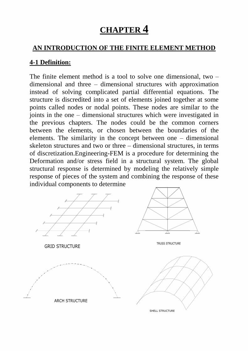
of discretization.Engineering-FEM is a procedure for determining the

Deformation and/or stress field in a structural system. The global

structural response is determined by modeling the relatively simple

response of pieces of the system and combining the response of these

individual components to determine the global response.

GRID STRUCTURETRUSS STRUCTURE

SHELL STRUCTURE

It is obvious that in one – dimensional structures the element is a one

– dimensional member. In two – dimensional structures, the element is

a two – dimensional plate or shell element. The three – dimensional

element could be a cube, prism, or a tetrahedron, either with straight

sides.

The solution of the finite element method is almost the same as the

direct stiffness matrix method. Once the elements stiffness matrices

are found, these matrices are augmented according to the

compatibility and equilibrium conditions at every node. The free nodal

displacements can be determined after specifying the boundary

conditions at the boundary nodes. However, what interests the

analysis in two – dimensional and three – dimensional structures is the

stresses and strains not forces and displacements. Therefore, it is

TWO DIMENSIONAL ELEMENTS

THREE DIMENSIONAL ELEMENTS

necessary to relate the strains at a point within the element with the

nodal displacements.

4-2 Course objectives:

Students will have the Knowledge and skills to use the finite element

method to predict stress and strain fields is elastic structural

subassemblies subjected to a variety of static load conditions.

1- Under stand the theory of the finite element method and

demonstrate this under standing by formulating the finite element

problem.

2- Solve a global structural analysis problem for a structure and

solution.

3- Use a typical finite element analysis soft ware package to analyze

structures and interpret the results of these analyses.

4-3 Mathematical view of the FEM:

It is a numerical method that provides an approximate solution to a

boundary value problem that is defined by a partial or ordinary

differential equation.

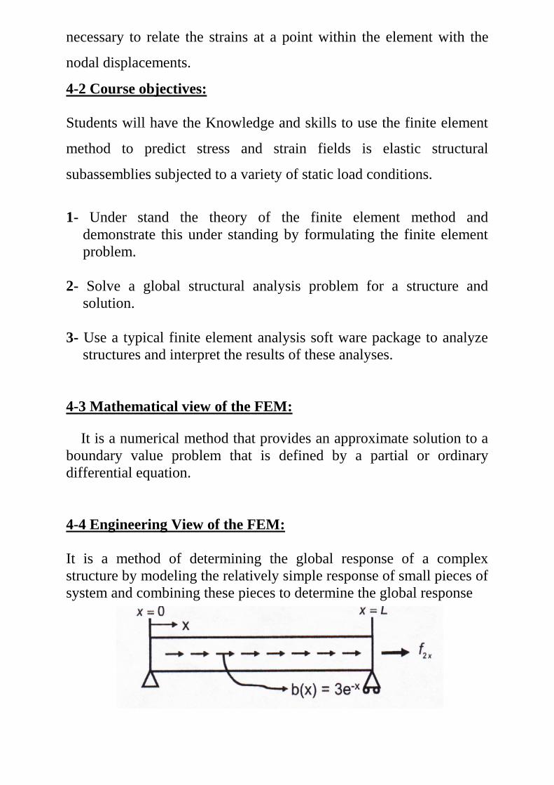
4-4 Engineering View of the FEM:

It is a method of determining the global response of a complex

structure by modeling the relatively simple response of small pieces of

system and combining these pieces to determine the global response

Element with constant area, elastic modulus and stress. We know the

relation ship between stress, strain and force for these simple

elements.

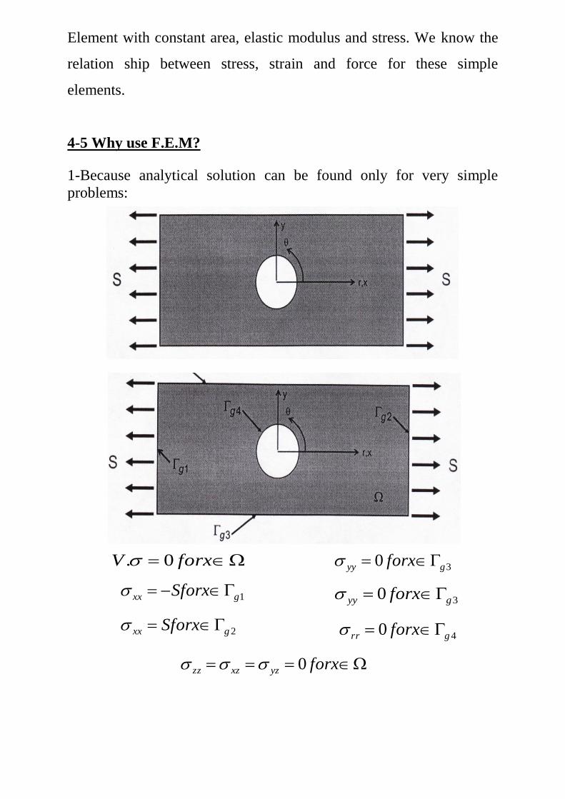
4-5 Why use F.E.M?

1-Because analytical solution can be found only for very simple

problems:

forxV 0.

1gxx Sforx

2gxx Sforx

30 gyy forx

30 gyy forx

40 grr forx

forxyzxzzz 0

2- It provides a tool for use in determining the response of complex

structures.

Wall frame systems Frame elements Plane stress or shell elements

3-Complex structures in the design office, Structural wall with

irregular openings subjected to simulated earthquake loading

cos3411

2 4

4

2

2

2

2

r

a

r

a

r

aSrr

2cos311

2 4

4

2

2

r

a

r

aS

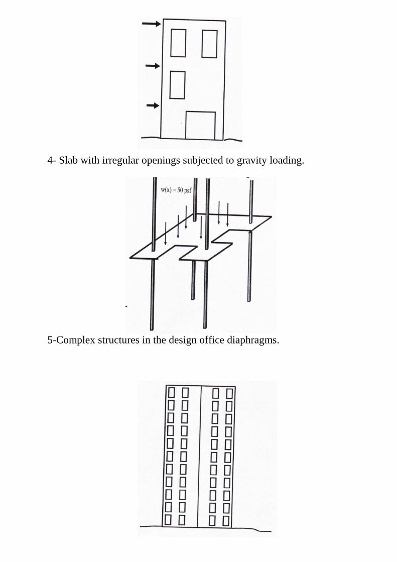
4- Slab with irregular openings subjected to gravity loading.

5-Complex structures in the design office diaphragms.

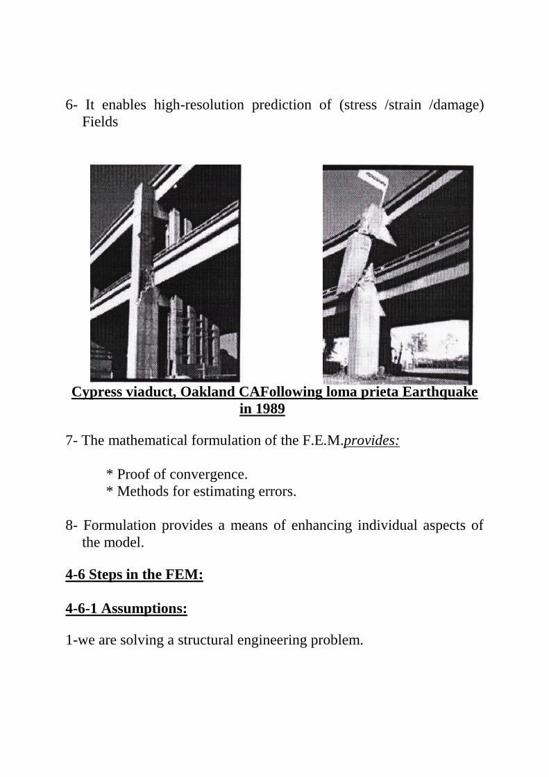
6- It enables high-resolution prediction of (stress /strain /damage)

Fields

Cypress viaduct, Oakland CAFollowing loma prieta Earthquake

in 1989

7- The mathematical formulation of the F.E.M.provides:

* Proof of convergence.

* Methods for estimating errors.

8- Formulation provides a means of enhancing individual aspects of

the model.

4-6 Steps in the FEM:

4-6-1 Assumptions:

1-we are solving a structural engineering problem.

2-The unknowns we seek are nodal displacements _ that define the

displacement along the edges of the pieces that compose the body.

From these we can compute strains and stresses.

3-The solution is a displacement field that satisfies equilibrium,

compatibility and constitutive requirements.

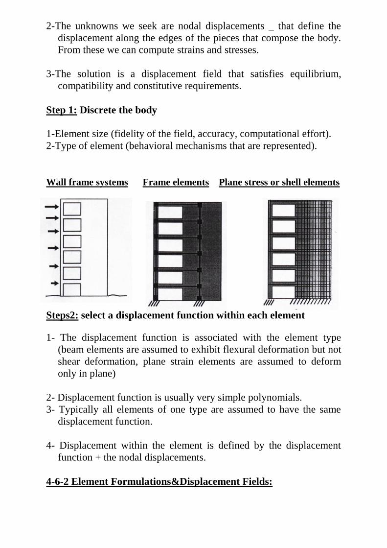
Step 1: Discrete the body

1-Element size (fidelity of the field, accuracy, computational effort).

2-Type of element (behavioral mechanisms that are represented).

Wall frame systems Frame elements Plane stress or shell elements

Steps2: select a displacement function within each element

1- The displacement function is associated with the element type

(beam elements are assumed to exhibit flexural deformation but not

shear deformation, plane strain elements are assumed to deform

only in plane)

2- Displacement function is usually very simple polynomials.

3- Typically all elements of one type are assumed to have the same

displacement function.

4- Displacement within the element is defined by the displacement

function + the nodal displacements.

4-6-2 Element Formulations&Displacement Fields:

1-DTruss Element (1 displacement D.O.F.per node in direction of bar

axis. Two nodal displacements enable definition of linear

displacement function)

2-D Frame element (1 displacements and 1 rotational D.O.F.per node

in the direction perpendicular to the axis of the element. Four nodal

(displacement) enable definition of a cubic displacement field).

2-D plan stress and plane strain Elements (2 orthogonal displacement

D.O.F. per node, displacement is linear in x&y with one cross

term).

Pseudo 3-D Axisymmetric Elements (2 orthogonal disp. D.O.F. per

node, within a plane displacement is linear in z&r with one cross

term).

Plate element (2 rotations and 1 out of – plan disp. D.O.F. per node.

the out of plan displacement field is cubic in x&y with cross terms).

Shell Elements (3 displacement and 2 rotation D.O.F. per node).

+

Out of plan bending In-plan (membrane) action

Step 3: Define the strain displacement (kinematics) and stress strain

relationships (constitution).

Step 4: Derive the element stiffness matrix and equilibrium equations

using direct equilibrium method _this is probably what you

have done so far. Or Work & Energy Method _ the principle

of minimum potential energy.Castiglianos theorem & the

principle of virtual work and method of weighted residual _

Galerkins method.

Step 5: Assemble the element equilibrium equations to obtain the

global equilibrium equations and introduce boundary

conditions.

F=K.D

Step 6: Solve for unknown nodal displacements.

step 7: Solve for element stresses and strains.

Step 8: Interpret the results.

4-7 Types of elements:

1- Beam Elements. (BE)

2- Triangle Elements. (ΔE)

3- Four Node Elements. (4NE)

4- Rectangle Elements. (RE)

5- Four Node Quadratic Elements. (4NQE)

6- Eight Node Quadratic Elements. (8NQE)

7- Four Node Quadratic Isoperimetric Elements. (4NQIE)

8- Friction Element. (FE)

9- Fracture Element. (CE)

10- Infinite Elements. (IE)

Example: Construct the Finite Element Mesh

4-8 The Unit Displacement Method:

The Unit Displacement Method (UDM) is used for computing the

stiffness matrix for truss and beam finite element models.

1 2

u1 u2

F1 F2

k

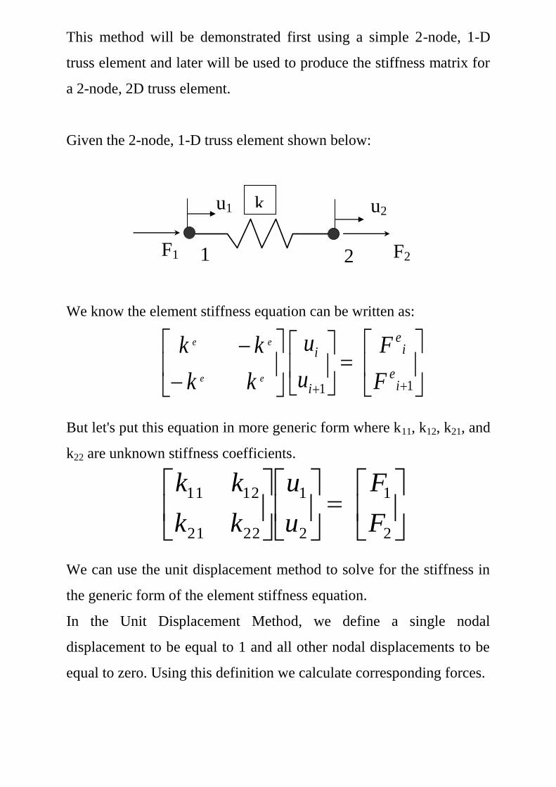
This method will be demonstrated first using a simple 2-node, 1-D

truss element and later will be used to produce the stiffness matrix for

a 2-node, 2D truss element.

Given the 2-node, 1-D truss element shown below:

We know the element stiffness equation can be written as:

But let's put this equation in more generic form where k11, k12, k21, and

k22 are unknown stiffness coefficients.

We can use the unit displacement method to solve for the stiffness in

the generic form of the element stiffness equation.

In the Unit Displacement Method, we define a single nodal

displacement to be equal to 1 and all other nodal displacements to be

equal to zero. Using this definition we calculate corresponding forces.

11

i

e

ie

i

i

F

F

u

u

kk

kk

ee

ee

2

1

2

1

2221

1211

F

F

u

u

kk

kk

1 2

u1 u2

F1 F2

k

IMPORTANT NOTE:

A unit displacement (=1) is assumed to be a very small

displacement which does not significantly change the geometry of

the element.

For the previous example, using the Unit Displacement Method, we

get:

u1=1

u2=0

Now use our Mechanics of Material equations assuming equilibrium

around the element where u1=1 and u2=0, we have:

or

Thus:

and

2

1

2

1

2221

1211

F

F

u

u

kk

kk

20*1*

0*1*

2221

11211

Fkk

Fkk

221

111

Fk

Fk

212

121

)(*

)(*

Fuuk

Fuuk

2

1

)10(*

)01(*

Fk

Fk

kF

kF

2

1

kk

kk

21

11

u1y

u2x

u2y

F1x

F1y

F2x

F2y

u1x

X

Y

Using the same logic but setting u1=0 and u2=1:

F1=k12=-k and F2=k22=k

Thus:

Repeat this method to determine the stiffness matrix for the 2-node, 2-

D truss element below:

Note, that a node could only move horizontally in the 1D truss

element, however, a node in a 2D truss element can move in the x- or

y-direction. We therefore say that the 1D truss element has 1 degree of

freedom (1DOF) per node while the 2D truss element has 2DOF’s per

node.

The four nodal equilibrium equations for the element can be written in

matrix form as:

kk

kk

kk

kk

2221

1211

u1x = 1 F1x

F1y

F2x

F2y

cos(

u2x=0

u2y=0

u1y=0

u1x = 1 F1x

F1y

F2x

F2y

cos(

u2x=0

u2y=0

u1y=0

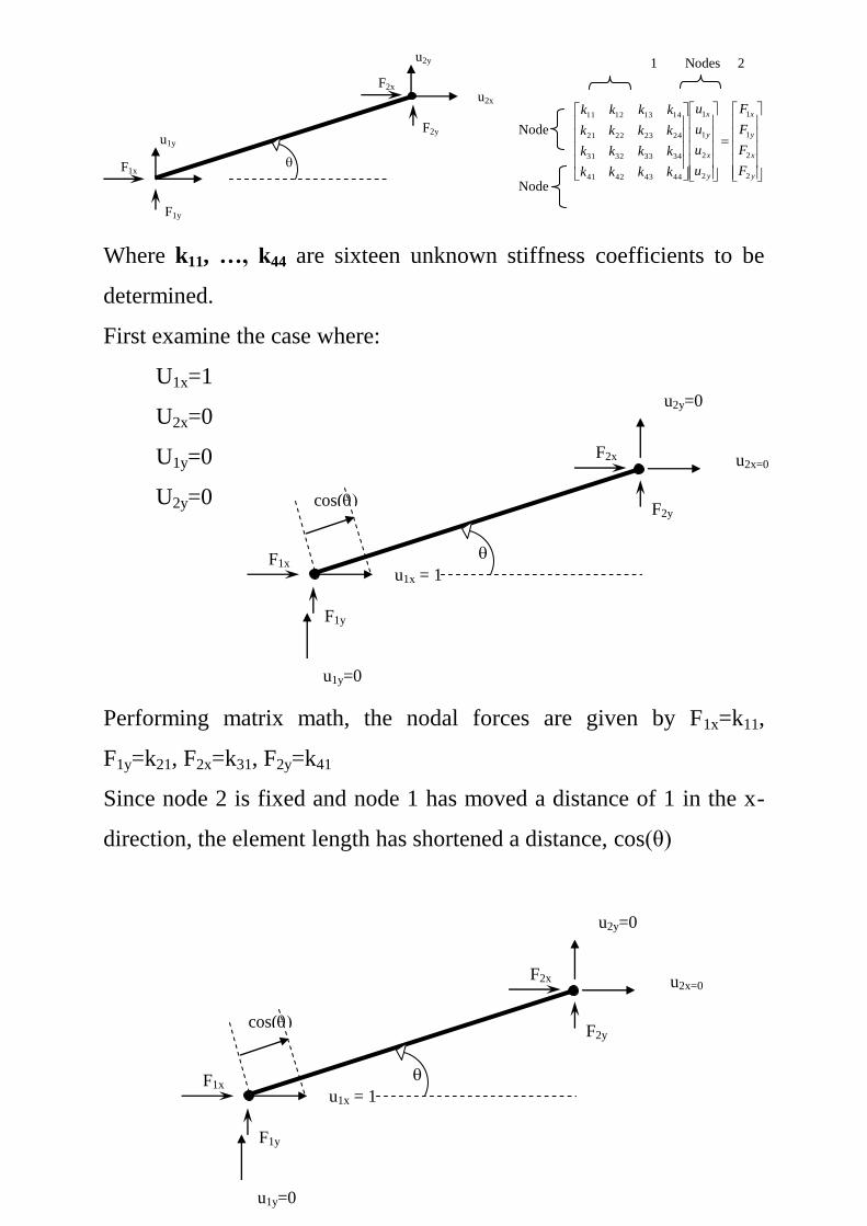
Where k11, …, k44 are sixteen unknown stiffness coefficients to be

determined.

First examine the case where:

U1x=1

U2x=0

U1y=0

U2y=0

Performing matrix math, the nodal forces are given by F1x=k11,

F1y=k21, F2x=k31, F2y=k41

Since node 2 is fixed and node 1 has moved a distance of 1 in the x-

direction, the element length has shortened a distance, cos(θ)

y

x

y

x

y

x

y

x

F

F

F

F

u

u

u

u

kkkk

kkkk

kkkk

kkkk

2

2

1

1

2

2

1

1

44434241

34333231

24232221

14131211

u1y

u2x

u2y

F1x

F1y

F2x

F2y

1 Nodes 2

x y x y

Node

1

Node

2

θ

Fe

F1Y

F1X

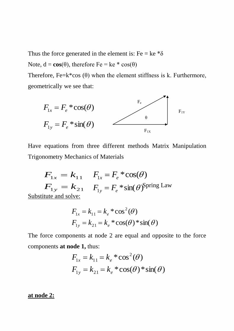
Thus the force generated in the element is: Fe = ke *δ

Note, d = cos(θ), therefore Fe = ke * cos(θ)

Therefore, Fe=k*cos (θ) when the element stiffness is k. Furthermore,

geometrically we see that:

Have equations from three different methods Matrix Manipulation

Trigonometry Mechanics of Materials

Spring Law

Substitute and solve:

The force components at node 2 are equal and opposite to the force

components at node 1, thus:

at node 2:

)cos(*1 ex FF

)sin(*1 ey FF

211

111

kF

kF

y

x

)cos(*1 ex FF

)sin(*1 ey FF

)sin(*)cos(*

)(cos*

211

2

111

ey

ex

kkF

kkF

)sin(*)cos(*

)(cos*

211

2

111

ey

ex

kkF

kkF

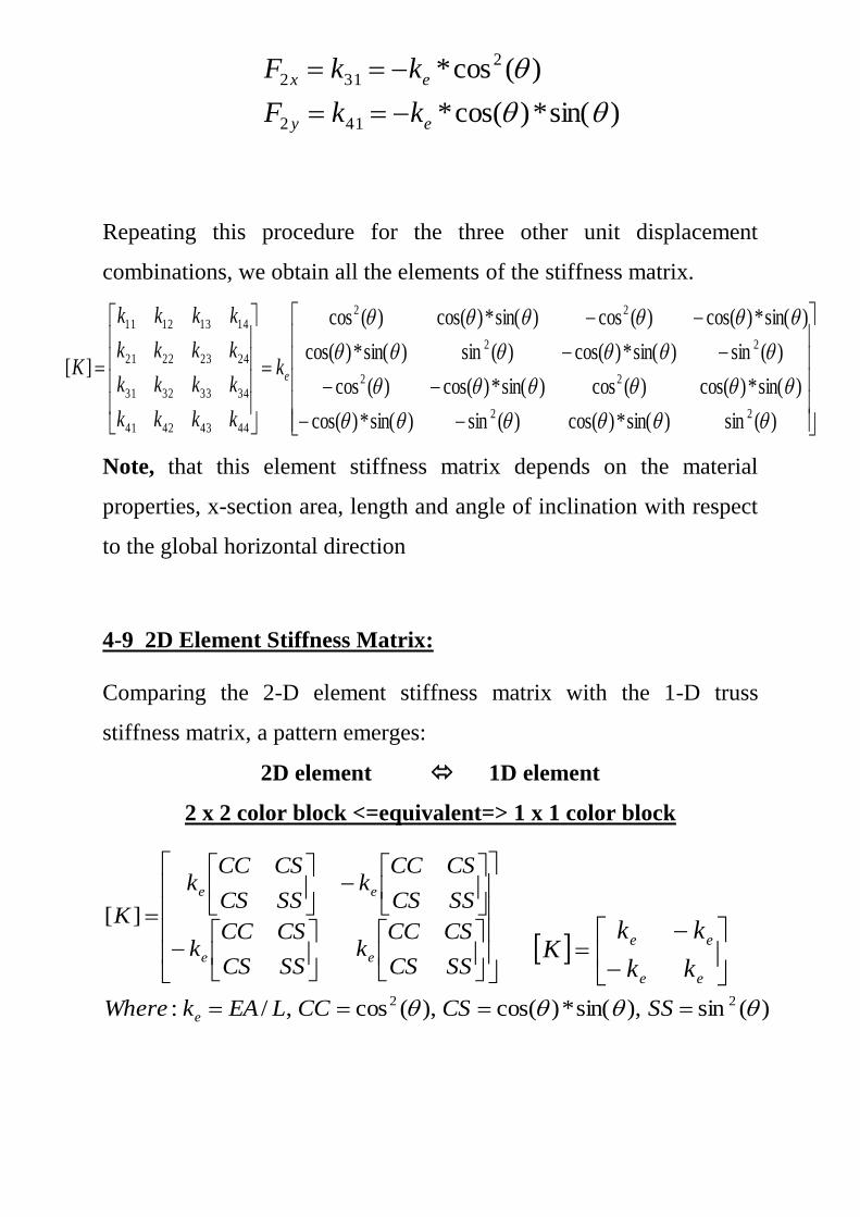
Repeating this procedure for the three other unit displacement

combinations, we obtain all the elements of the stiffness matrix.

Note, that this element stiffness matrix depends on the material

properties, x-section area, length and angle of inclination with respect

to the global horizontal direction

4-9 2D Element Stiffness Matrix:

Comparing the 2-D element stiffness matrix with the 1-D truss

stiffness matrix, a pattern emerges:

2D element 1D element

2 x 2 color block <=equivalent=> 1 x 1 color block

)sin(*)cos(*

)(cos*

412

2

312

ey

ex

kkF

kkF

)(sin)sin(*)cos()(sin)sin(*)cos(

)sin(*)cos()(cos)sin(*)cos()(cos

)(sin)sin(*)cos()(sin)sin(*)cos(

)sin(*)cos()(cos)sin(*)cos()(cos

][

22

22

22

22

44434241

34333231

24232221

14131211

ek

kkkk

kkkk

kkkk

kkkk

K

)(sin),sin(*)cos(),(cos,/:

][

22

SSCSCCLEAkWhere

SSCS

CSCCk

SSCS

CSCCk

SSCS

CSCCk

SSCS

CSCCk

K

e

ee

ee

ee

ee

kk

kkK

Therefore, the 2D element stiffness matrix is comprised of one 2 x 2

block matrix [kb] arranged so that:

and the 2 x 2 block matrix [kb] is defined by:

4-10 3D Element Stiffness Matrix:

For a 3D truss element, the element stiffness matrix the mathematical

structure of [K] is the same as for the 2D element:

Where [kb] is a 3x3 block matrix and [K] is a 6 x 6 element stiffness

matrix.

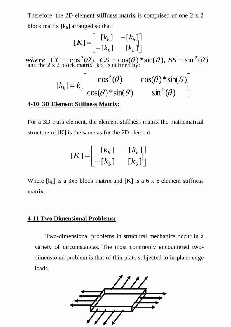
4-11 Two Dimensional Problems:

Two-dimensional problems in structural mechanics occur in a

variety of circumstances. The most commonly encountered two-

dimensional problem is that of thin plate subjected to in-plane edge

loads.

)(sin),sin(*)cos(),(cos

][][

][][][

22

SSCSCCwhere

kk

kkK

bb

bb

)(sin)sin(*)cos(

)sin(*)cos()(cos][

2

2

eb kk

][][

][][][

bb

bb

kk

kkK

Triangular elements

Quadrilateral elements

Two-dimensional domain

4-11-1 Two Dimensional Elements:

Two-dimensional problems are typically modeled using triangular

or quadrilateral elements.

4-12 Beam Element:

Beam elements are commonly used in the modeling of skeletal

structures. One may use either plane or space elements according to

the structure to be analyzed. Only plane element is introduced in this

thesis, as in our analysis we are encountered by plane problems in

which the element models the conduit walls.

The plane beam element has 2 nodes, one at each of its ends. At

each node, 3 degrees of freedom exist. The degrees of freedom are

horizontal displacement, vertical displacement and rotation from

horizontal to vertical direction. The element have six degrees of

freedom consequently, the element stiffness matrix is (6 * 6) matrix.

The formulation of stiffness matrix develops from the physical

meaning of the matrix elements. Let kij be the value of the element in

row no. i and column no. j. This value represents the force induced in

the direction of freedom no. i due to a unit displacement in the

direction of degree of freedom no. j while the other degree of freedom

are restricted. Hence, the end forces resulting from the previous

displacement configuration are the values of column j in the stiffness

matrix.

Let us consider a beam element, in a general position, inclined to the

X-axis by an angle 0 (positively measured in the counter – clockwise

sense). Also let the properties of the element material are:

E: Young's modulus of the element material.

I: second moment of area of the cross – section about the axis

perpendicular to the plane of element and passes through the

centroid of the cross – section.

A: Cross sectional area.

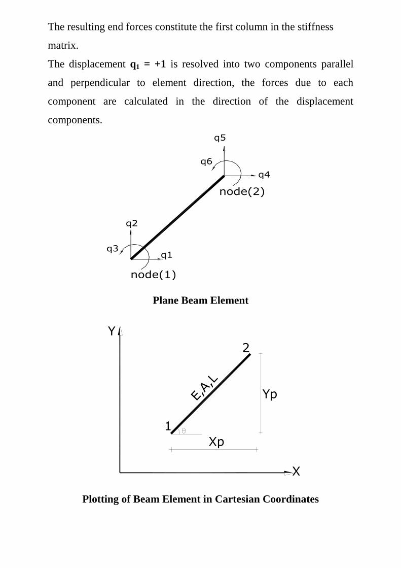
Furthermore, the coordinates of the element nodes are (X1, Y1)

and(X2, Y2). Then the projections of the element along X and Y axes

are Xp and Yp respectively.

Xp = X2 - X1

Yp = Y2 - Y1

The element length L =

Now a unit displacement (positive) is given to the degree of freedom,

q1 whereas degrees q2 and q6 restricted.

22 )()[( pp YX

node(1)

node(2)

q5

q4

q6

q2

q3q1

Y

X

E,A,L

1

2

Xp

Yp

The resulting end forces constitute the first column in the stiffness

matrix.

The displacement q1 = +1 is resolved into two components parallel

and perpendicular to element direction, the forces due to each

component are calculated in the direction of the displacement

components.

Plane Beam Element

Plotting of Beam Element in Cartesian Coordinates

2

3

3

22

2

3

3

22

sin6

cossin12cossin

sin12cos

sin6

cossin12cossin

sin12cos

L

EIL

EI

L

EAL

EI

L

EAL

EIL

EI

L

EAL

EI

L

EA

K =

C X + C Y1 p

2

2 p

2

C X Y - C X Y1 p 2 pp p

- C Y L2 p

2

2

- C X - C Y1 p

2

2 p

2

- C X Y + C X Y1 p 2 pp p

- C Y L2 p

2

2

C X Y - C X Y1 p 2 pp p

- C Y - C X1 p

2

2 p

2

C X L2 p

2

2

- C X Y + C X Y1 p 2 pp p

- C Y - C X1 p

2

2 p

2

C X L2 p

2

2

- C Y L2 p

2

2

C X L2 p

2

2

-4EI / L

C Y L2 p

2

2

- C X L2 p

2

2

2EI / L

- C X - C Y1 p

2

2 p

2

- C X Y +C X Y1 p 2 pp p

C Y L2 p

2

2

C X + C Y1 p

2

2 p

2

C X Y - C X Y1 p 2 pp p

C Y L2 p

2

2

- C X Y + C X Y1 p 2 pp p

- C Y - C X1 p

2

2 p

2

- C X L2 p

2

2

- C X Y + C X Y1 p 2 pp p

C Y + C X1 p

2

2 p

2

- C X L2 p

2

2

- C Y L2 p

2

2

C X L2 p

2

2

2EI / L

C Y L2 p

2

2

- C X L2 p

2

2

4EI / L

The forces due to the two components are added together. Then

resolved in the directions of the original degrees of freedom.

Hence, the first column is:

Similarly, unit displacement is given to the degrees q2, q3, q4, q5, q6 one

by one and keeping the other degrees restricted.

The end forces can be related to end displacements as follows:

N1 = (D4 – D1) * E* A/L = E *A /L (D4 – D1)

N2 = N1

Q1 = 12 E * I / L3

(D2-D5) +6 E * I /L2 ( D6 – D3)

Q1 = Q2

M1 = 6 E * I /L2 ( D5 – D2) - 2 E * I / L (D6 + 2D3)

M2 = 6 E * I /L2 ( D2 – D5) - 2 E * I / L (D3 + 2D6)

xj

X

i

j

qi

vj

vi

qj

xi

pi

uj

ui

k uk

vk

pj

qk

pk

Y

xk

yi

yj

yk

T

kkjjii vuvuvuu ][

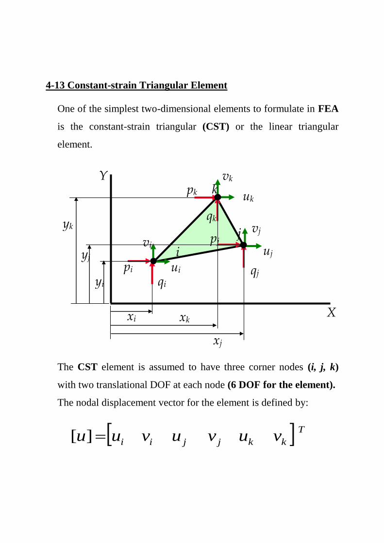
4-13 Constant-strain Triangular Element

One of the simplest two-dimensional elements to formulate in FEA

is the constant-strain triangular (CST) or the linear triangular

element.

The CST element is assumed to have three corner nodes (i, j, k)

with two translational DOF at each node (6 DOF for the element).

The nodal displacement vector for the element is defined by:

The locations of the nodes are defined by x and y coordinates

relative to a global reference frame. The triangle can have arbitrary

proportions as defined by the locations of its nodes.

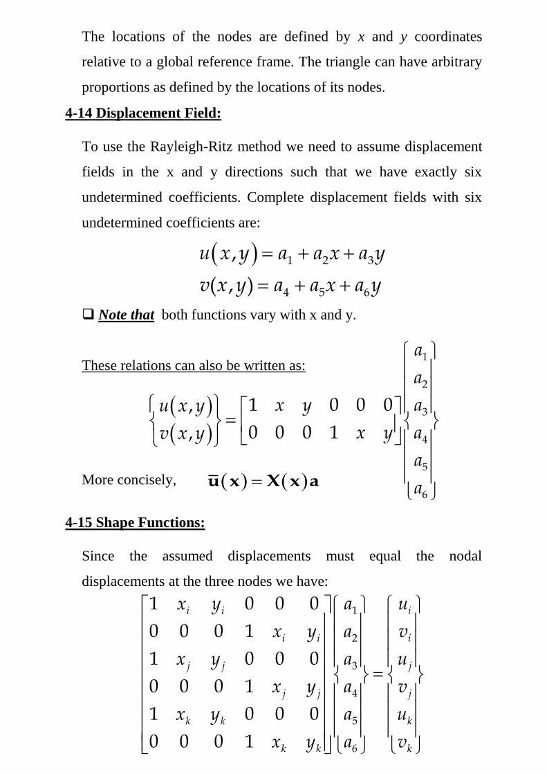
4-14 Displacement Field:

To use the Rayleigh-Ritz method we need to assume displacement

fields in the x and y directions such that we have exactly six

undetermined coefficients. Complete displacement fields with six

undetermined coefficients are:

Note that both functions vary with x and y.

These relations can also be written as:

More concisely,

4-15 Shape Functions:

Since the assumed displacements must equal the nodal

displacements at the three nodes we have:

1 2 3

4 5 6

,

( , )

u x y a a x a y

v x y a a x a y

1

2

3

4

5

6

1 0 0 0,

0 0 0 1,

a

a

x y au x y

x y av x y

a

a

u x X x a

1

2

3

4

5

6

1 0 0 0

0 0 0 1

1 0 0 0

0 0 0 1

1 0 0 0

0 0 0 1

i i i

i i i

j j j

j j j

k k k

k k k

x y a u

x y a v

x y a u

x y a v

x y a u

x y a v

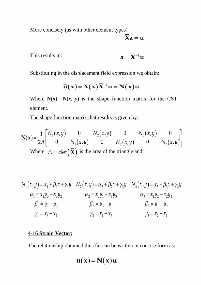
More concisely (as with other element types)

This results in:

Substituting in the displacement field expression we obtain:

Where N(x) =N(x, y) is the shape function matrix for the CST

element.

The shape function matrix that results is given by:

Where is the area of the triangle and:

4-16 Strain Vector:

The relationship obtained thus far can be written in concise form as:

Xa u

1a X u

1 u x X x X u N x u

1 2 3

1 2 3

, 0 , 0 , 01

0 , 0 , 0 ,2

N x y N x y N x y

N x y N x y N x yA

N x

detA X

1 1 1 1 2 2 2 2 3 3 3 3

1 2 3 3 2 2 3 1 1 3 3 1 2 2 1

1 2 3 2 3 1 3 1 2

1 3 2 2 1 3 3 2 1

, , ,N x y x y N x y x y N x y x y

x y x y x y x y x y x y

y y y y y y

x x x x x x

u x N x u

x

N

y

N

x

N

y

N

x

N

y

N

y

N

y

N

y

N

x

N

x

N

x

N

B

332211

321

321

000

000

][

332211

321

321

000

000

2

1][

AB

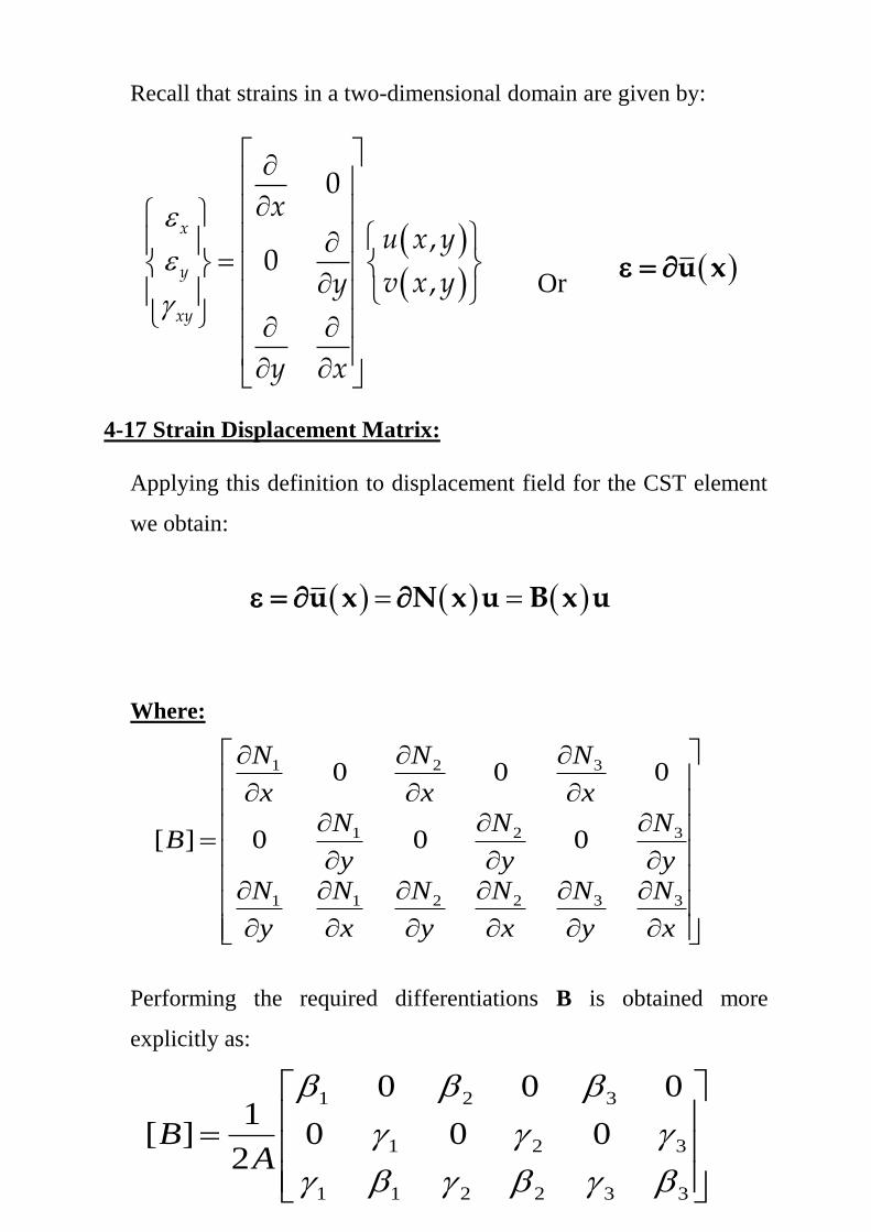
Recall that strains in a two-dimensional domain are given by:

Or

4-17 Strain Displacement Matrix:

Applying this definition to displacement field for the CST element

we obtain:

Where:

Performing the required differentiations B is obtained more

explicitly as:

0

,0

,

x

y

xy

xu x y

v x yy

y x

u x

u x N x u B x u

2

100

01

01

1][

2

EE

2

2100

01

01

)21)(1(][

EE

Where and have the same definitions as those in N Clearly the

strain-displacement matrix B is a constant matrix (no dependence

on x or y)

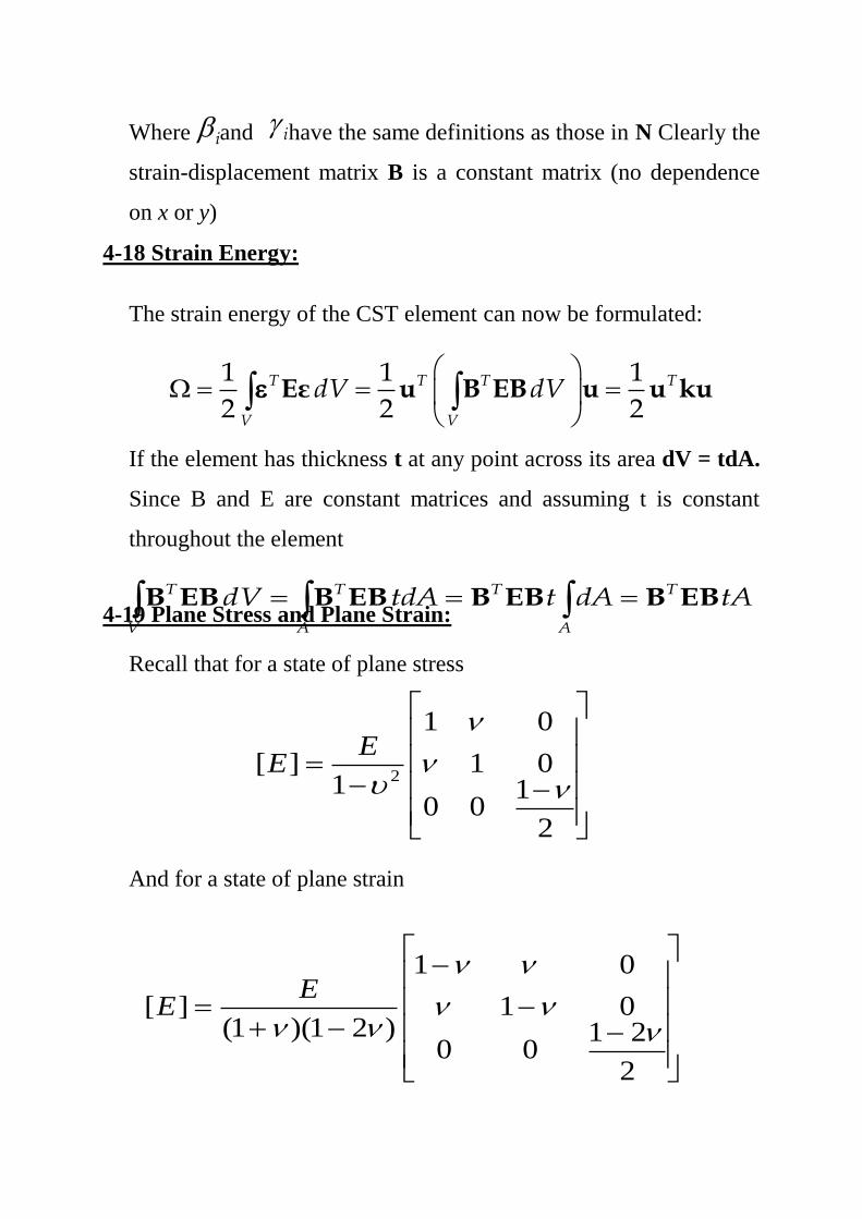
4-18 Strain Energy:

The strain energy of the CST element can now be formulated:

If the element has thickness t at any point across its area dV = tdA.

Since B and E are constant matrices and assuming t is constant

throughout the element

4-19 Plane Stress and Plane Strain:

Recall that for a state of plane stress

And for a state of plane strain

i i

1 1 1

2 2 2T T T T

V V

dV dV

Eε u B EB u u ku

T T T T

V A A

dV tdA t dA tA B EB B EB B EB B EB

X

i j vi

pi ui

k Y

l

m n

2 21 2 3 4 5 6

2 27 8 9 10 11 12

,

( , )

u x y a a x a y a x a xy a y

v x y a a x a y a x a xy a y

maxmax

min min

12 312 12 3 3 3 12yx

T

x y

t dx dy

k B E B

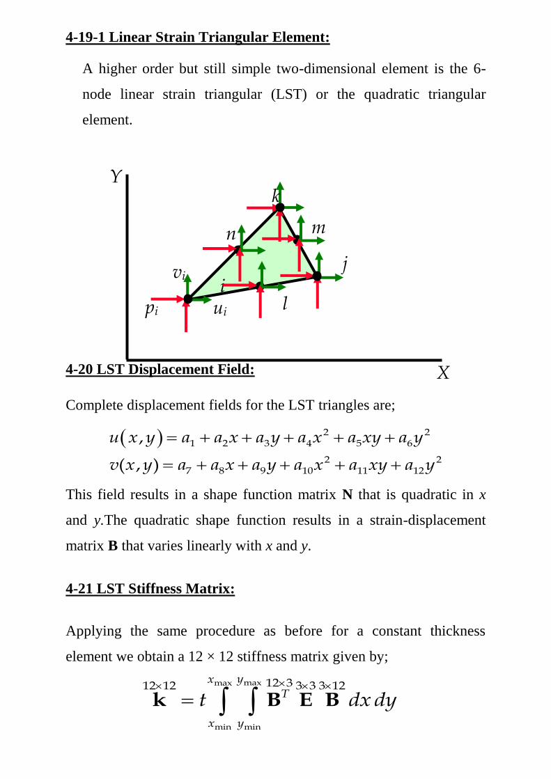
4-19-1 Linear Strain Triangular Element:

A higher order but still simple two-dimensional element is the 6-

node linear strain triangular (LST) or the quadratic triangular

element.

4-20 LST Displacement Field:

Complete displacement fields for the LST triangles are;

This field results in a shape function matrix N that is quadratic in x

and y.The quadratic shape function results in a strain-displacement

matrix B that varies linearly with x and y.

4-21 LST Stiffness Matrix:

Applying the same procedure as before for a constant thickness

element we obtain a 12 × 12 stiffness matrix given by;

1A

2A

3A

j

k

l

m

n

1 2 3 1L L L

1 1

1 2

0 0

Tt dL dL k B EB

The integration shown is in general laborious to perform analytically;

as a result a numerical method such as Gaussian quadrature is used to

obtain the matrix

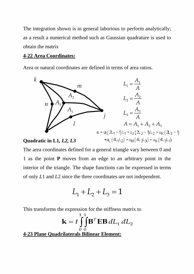
4-22 Area Coordinates:

Area or natural coordinates are defined in terms of area ratios.

Quadratic in L1, L2, L3

The area coordinates defined for a general triangle vary between 0 and

1 as the point P moves from an edge to an arbitrary point in the

interior of the triangle. The shape functions can be expressed in terms

of only L1 and L2 since the three coordinates are not independent.

This transforms the expression for the stiffness matrix to

4-23 Plane Quadrilaterals Bilinear Element:

11

22

33

1 2 3

AL

AA

LAA

LA

A A A A

xj

X

i

j

qi

vj

vi

qj

xi

pi

uj

ui

k uk

vk

pj

qk

pk

Y

xk

yi

yj

yl

ul

l vl

ql

pl

yk

xl

1 2 3 4

5 6 7 8

,

( , )

u x y a a x a y a xy

v x y a a x a y a xy

1a X u

1 u x X x X u N x u

The 4-node quadrilateral element is the simplest four-sided two-

dimensional element

4-23-1 Bilinear Displacement Field:

The assumed displacement field for this element is

Or

Note that the assumed displacement field is not “complete” (neither

linear nor quadratic).Writing these expressions more concisely and

performing the usual operations we obtain;

1

2

3

4

5

6

7

8

1 0 0 0 0,

0 0 0 0 1,

a

a

a

x y xy au x y

x y xy av x y

a

a

a

Xa u

1 2 3 4

1 2 3 4

, 0 , 0 , 0 , 0

0 , 0 , 0 , 0 ,

N x y N x y N x y N x y

N x y N x y N x y N x y

N x

u x N x u B x u

,

x x

y y

xy xy

y

x

x y

x

N

y

N

x

N

y

N

x

N

y

N

y

N

y

N

y

N

x

N

x

N

x

N

B

332211

321

321

000

000

][

Where N(x) =N(x, y) is the shape function matrix for the plane

quadrilateral bilinear (PQB) element

4-23-2 PQB Strain-Displacement Matrix:

The strain in this element can now be computed from;

Where:

Note that because of the assumed displacement field;

maxmax

min min

8 38 8 3 3 3 8yx

T

x y

h dx dy

k B E B

X

Y s

t

1

1

s

t

1

1

s

t

1

1

s

t

1

1

s

t

1

2t

1

2s

1 1

1 1

Th dsdt

k B EB

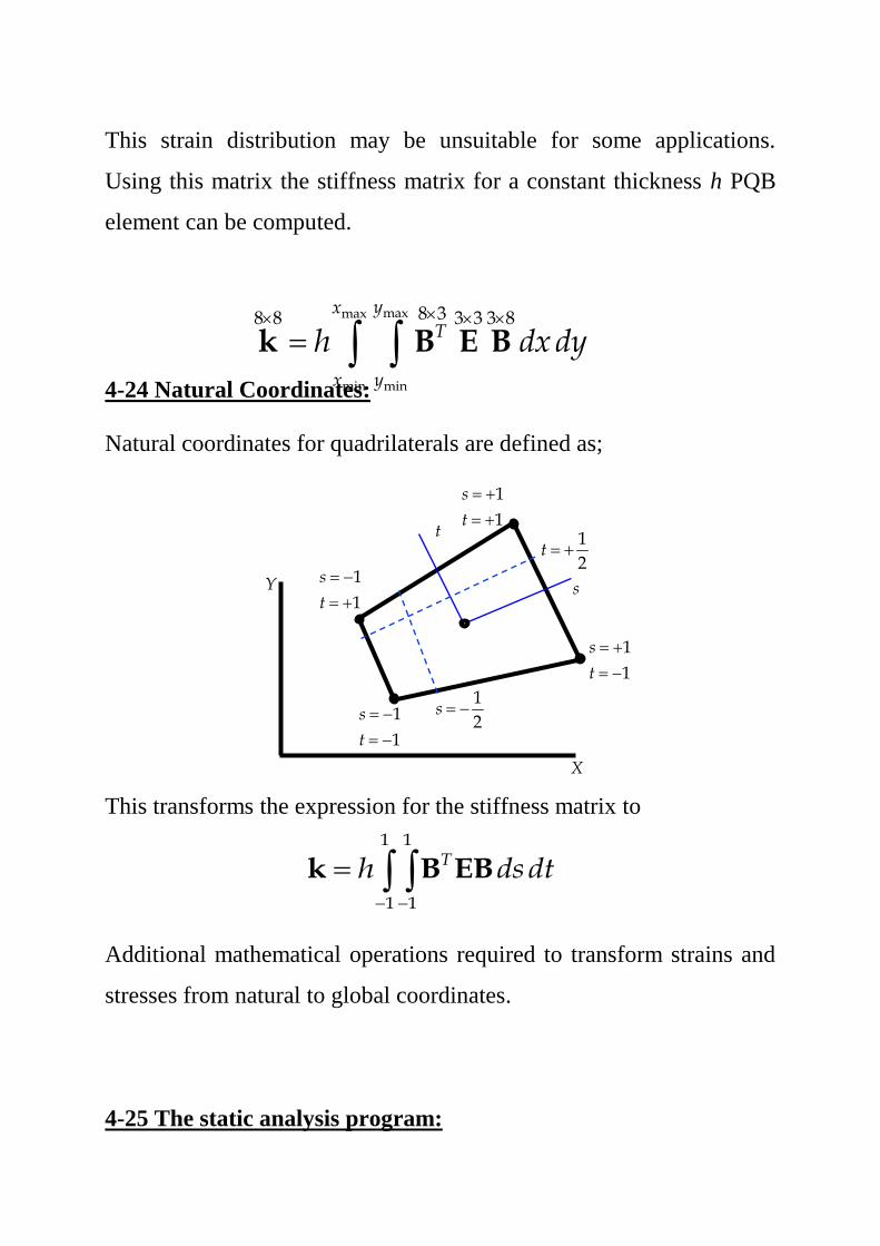
This strain distribution may be unsuitable for some applications.

Using this matrix the stiffness matrix for a constant thickness h PQB

element can be computed.

4-24 Natural Coordinates:

Natural coordinates for quadrilaterals are defined as;

This transforms the expression for the stiffness matrix to

Additional mathematical operations required to transform strains and

stresses from natural to global coordinates.

4-25 The static analysis program:

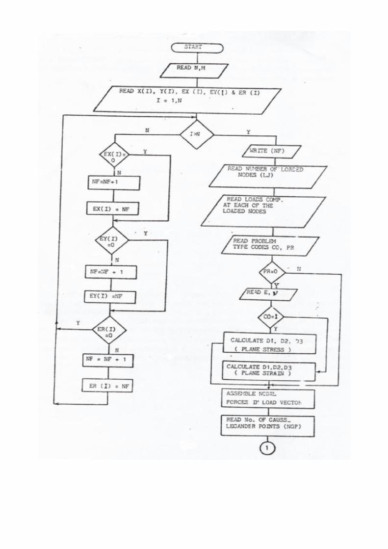
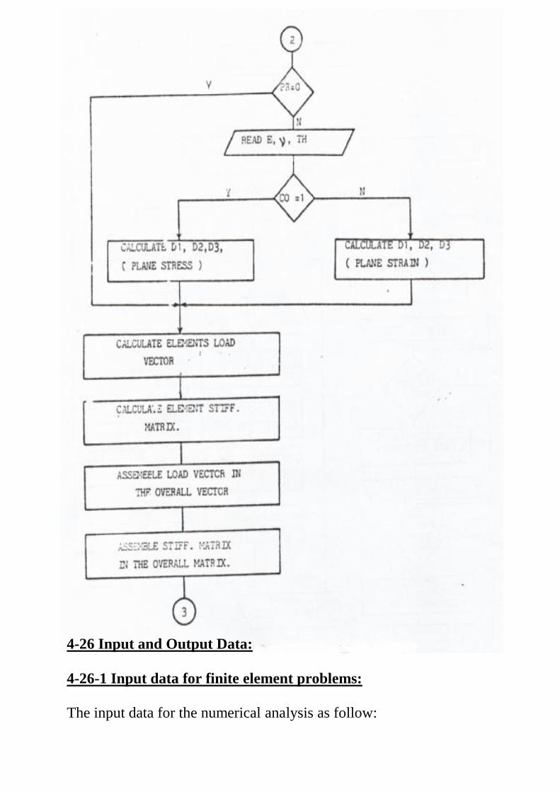
4-26 Input and Output Data:

4-26-1 Input data for finite element problems:

The input data for the numerical analysis as follow:

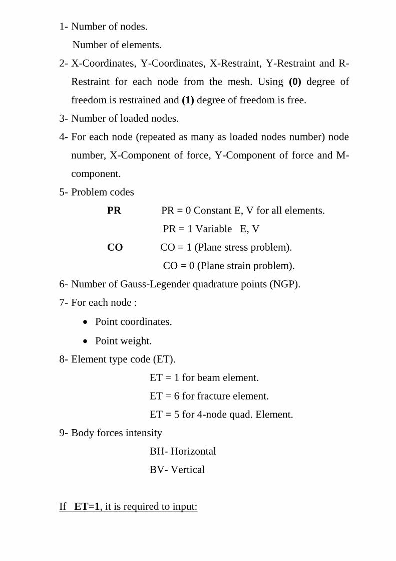
1- Number of nodes.

Number of elements.

2- X-Coordinates, Y-Coordinates, X-Restraint, Y-Restraint and R-

Restraint for each node from the mesh. Using (0) degree of

freedom is restrained and (1) degree of freedom is free.

3- Number of loaded nodes.

4- For each node (repeated as many as loaded nodes number) node

number, X-Component of force, Y-Component of force and M-

component.

5- Problem codes

PR PR = 0 Constant E, V for all elements.

PR = 1 Variable E, V

CO CO = 1 (Plane stress problem).

CO = 0 (Plane strain problem).

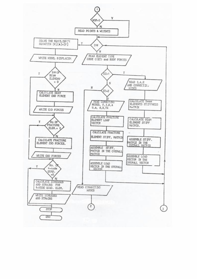
6- Number of Gauss-Legender quadrature points (NGP).

7- For each node :

Point coordinates.

Point weight.

8- Element type code (ET).

ET = 1 for beam element.

ET = 6 for fracture element.

ET = 5 for 4-node quad. Element.

9- Body forces intensity

BH- Horizontal

BV- Vertical

If ET=1, it is required to input:

10-Connecting nodes.

11-Inertia, Area, E.

If ET=6, it is required to input:

12- Connecting nodes.

13- Inertia, Area, E, V, crack-depth, depth of lining, breadth of

lining and crack code (TA = 1 crack upper and TA = 0 crack

lower).

If ET=5, it is required to input:

14- E, V, TH.

15- Connecting nodes in anticlockwise direction.

4-26-2 Output data for finite element problems:

The output data for each run were:

1- Number of nodes and number of elements.

2- CO and PR.

3- E, V and TH for soil medium.

4- Half band width.

5- Nodal displacements in tabulated form ( Randyx , ).

6- End forces of beam element (N.F, S.F and B.M) if any.

7- End forces of fracture of beam element (N.F, S.F and B.M) if

any.

8- Stress and strain for 4-node quad. Elements

( xyyxxyyx ,,,,, ) in a tabulated form.

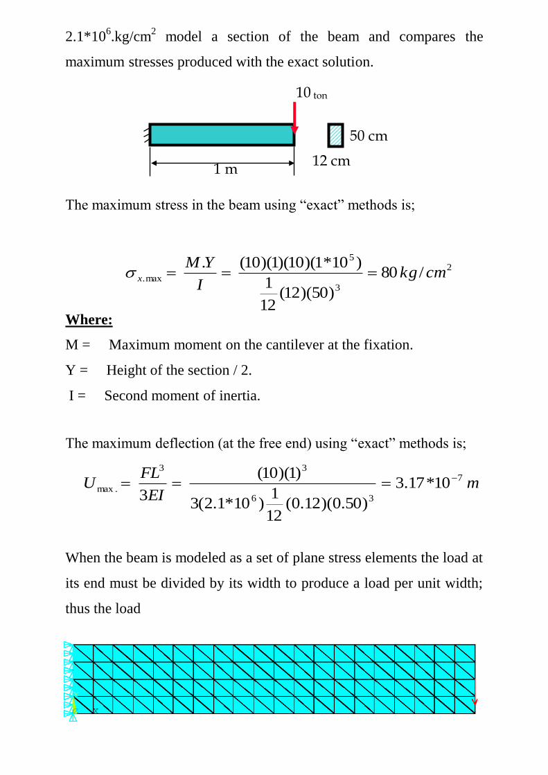
Example(1): Cantilever beam model by using finite element

method (2D element).

A cantilevered beam 1 m long, 12 cm wide and 50 cm high is loaded

by an end load of 10 ton. The Young’s modulus for the material is

1 m

10 ton

12 cm

50 cm

2

3

5

max. /80

)50)(12(12

1

)10*1)(10)(1)(10(.cmkg

I

YMx

mEI

FLU 7

36

33

.max 10*17.3

)50.0)(12.0(12

1)10*1.2(3

)1)(10(

3

2.1*106.kg/cm

2 model a section of the beam and compares the

maximum stresses produced with the exact solution.

The maximum stress in the beam using “exact” methods is;

Where:

M = Maximum moment on the cantilever at the fixation.

Y = Height of the section / 2.

I = Second moment of inertia.

The maximum deflection (at the free end) using “exact” methods is;

When the beam is modeled as a set of plane stress elements the load at

its end must be divided by its width to produce a load per unit width;

thus the load

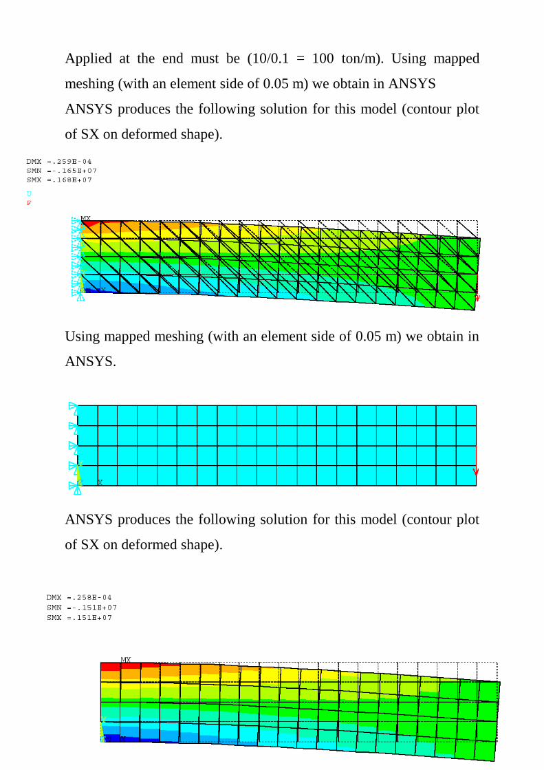
Applied at the end must be (10/0.1 = 100 ton/m). Using mapped

meshing (with an element side of 0.05 m) we obtain in ANSYS

ANSYS produces the following solution for this model (contour plot

of SX on deformed shape).

Using mapped meshing (with an element side of 0.05 m) we obtain in

ANSYS.

ANSYS produces the following solution for this model (contour plot

of SX on deformed shape).

16.00

8.00

4.00

4.00

4.00

(-ve column crack)

(mid-span crack)

SOIL MEDIUM

4.00 4.00 4.00 8.00

a

a

The second mapped mesh element provides a better approximation

with fewer elements and D.O.F than the first element in this case

because the stress variation in the y direction is linear in the exact

solution.

The first mapped mesh element may provide a better approximation in

instances when the bending moment varies quadratically or at a higher

order in the x direction.

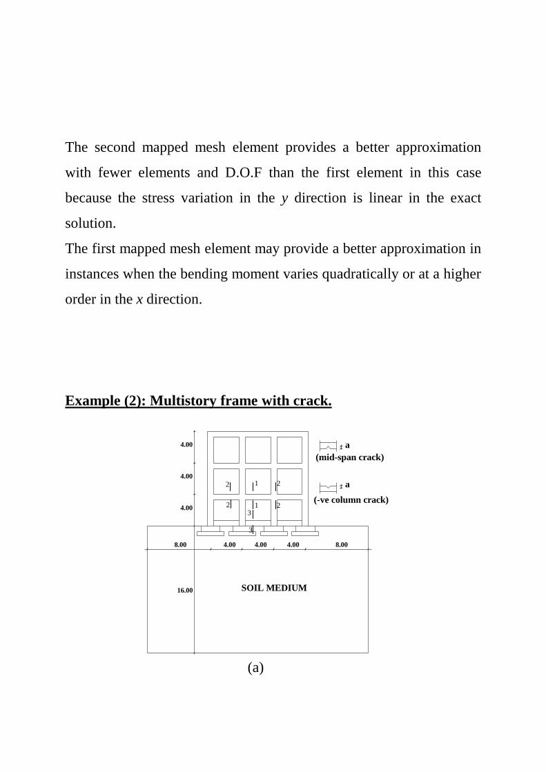
Example (2): Multistory frame with crack.

(a)

1

1

2

2 2

2

3

3

4.00

4.00

4.00

16.00

8.00 8.004.004.004.00

SOIL MEDIUM

a

a

(mid-span crack)

(-ve column crack)

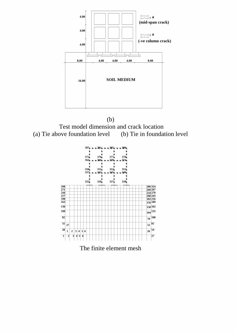
(b)

Test model dimension and crack location

(a) Tie above foundation level (b) Tie in foundation level

The finite element mesh

1 2 3 4 5 6 27

1 2 3 4 5 6 2628

55

82

109

136

163

190

217

244

271

298

54

81

108

135

162

189

216

243

270

297

324

325 326 327 328

337 341 345 349

350

362

351

366

352

370

353

374

387

375 376

391 399395

378377

27 52

78

104

130

156

182

208234

260

286

a/d = 0.6

a/d = 0.2

a/d = 0.0

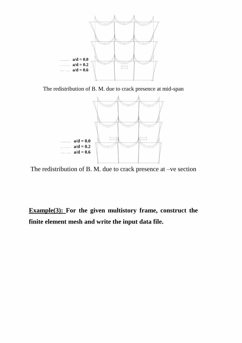
The redistribution of B. M. due to crack presence at mid-span

The redistribution of B. M. due to crack presence at –ve section

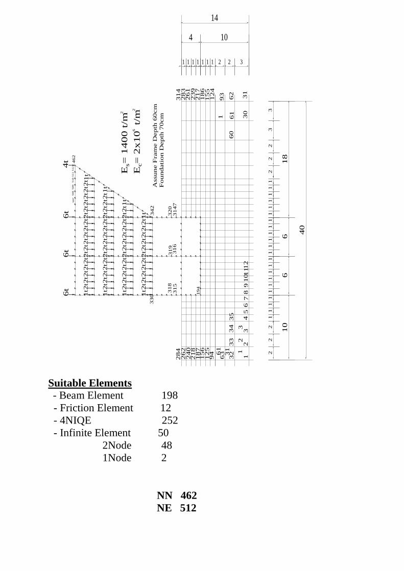
Example(3): For the given multistory frame, construct the

finite element mesh and write the input data file.

a/d = 0.0

a/d = 0.2

a/d = 0.6

1t2

t2t2

t2t2

t2t2

t2t2

t2t2

t2t2

t2t2

t2t2

t 1t

2t

2t

2t2

t2t2

t2t2

t2t2

t2t2

t2t2

t2t2

t2t

2t2

t2t2

t2t2

t2t2

t2t2

t2t2

t

2t2

t2t2

t2t2

t2t2

t2t2

t

1t

1t

1t

1t

1t

1t

6t

6t

6t

4t

33

22

21

11

11

11

11

11

11

11

11

11

11

12

22

1 1 1 1 1 1 1 2 2 3

14

4 10

18

66

10

40

12

34

56

78

91

0 111

23

03

1

32

33

34

35

63

94

12

51

56

18

72

18

24

02

62

28

4

19

3

12

41

55

18

62

17

23

92

61

28

33

14

62

61

60

46

2

315

316

31

47

318

319

320

330

342

12

3

31

61

512

511

510

509

508

507

19

4

E =

1400 t

/ms

2

E =

2x10 t/

mc

26

Assune F

ram

e D

epth

60cm

Foundati

on D

epth

70cm

Suitable Elements

- Beam Element 198

- Friction Element 12

- 4NIQE 252

- Infinite Element 50

2Node 48

1Node 2

NN 462

NE 512

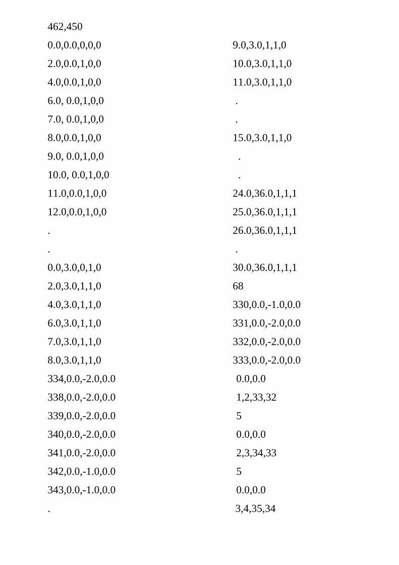
462,450

0.0,0.0,0,0,0 9.0,3.0,1,1,0

2.0,0.0,1,0,0 10.0,3.0,1,1,0

4.0,0.0,1,0,0 11.0,3.0,1,1,0

6.0, 0.0,1,0,0 .

7.0, 0.0,1,0,0 .

8.0,0.0,1,0,0 15.0,3.0,1,1,0

9.0, 0.0,1,0,0 .

10.0, 0.0,1,0,0 .

11.0,0.0,1,0,0 24.0,36.0,1,1,1

12.0,0.0,1,0,0 25.0,36.0,1,1,1

. 26.0,36.0,1,1,1

. .

0.0,3.0,0,1,0 30.0,36.0,1,1,1

2.0,3.0,1,1,0 68

4.0,3.0,1,1,0 330,0.0,-1.0,0.0

6.0,3.0,1,1,0 331,0.0,-2.0,0.0

7.0,3.0,1,1,0 332,0.0,-2.0,0.0

8.0,3.0,1,1,0 333,0.0,-2.0,0.0

334,0.0,-2.0,0.0 0.0,0.0

338,0.0,-2.0,0.0 1,2,33,32

339,0.0,-2.0,0.0 5

340,0.0,-2.0,0.0 0.0,0.0

341,0.0,-2.0,0.0 2,3,34,33

342,0.0,-1.0,0.0 5

343,0.0,-1.0,0.0 0.0,0.0

. 3,4,35,34

0,9 1,1 1,3 1,5 1,7 1,9

Are

a1 =

0.4

5X1=

0.45

m

1m

Are

a2 =

0.5

5X1=

0.5

5 m

Are

a3 =

0.6

5X1=

0.6

5 m

Are

a4 =

0.7

5X1=

0.75

m

Are

a5 =

0.8

5X1=

0.85

m

Are

a6 =

0.9

5X1=

0.95

m

2 2 2 2 2 2

Iner

tia =

0.4

5^3x

1/12

= 0.

0076

m

Iner

tia =

0.5

5^3x

1/12

= 0.

014

m

Iner

tia =

0.6

5^3x

1/12

= 0.

023

m

Iner

tia =

0.7

5^3x

1/12

= 0.

035

m

Iner

tia =

0.8

5^3x

1/12

= 0.

051

m

Iner

tia =

0.9

5^3x

1/12

= 0.

071

m

4 4 4 4 4 4

Are

a =

0.80

X1=

0.80

m Iner

tia =

0.8

0^3x

1/12

= 0.

042

m

2

4

1,6

2 2 2 2 2 2

Forc

e1 =

0.1

25 t

Forc

e1 =

1.0

t

Forc

e1 =

2.0

476

t

Forc

e1 =

1.3

274

t

Wat

er L

oads

, Are

a And

Iner

tia C

alcu

latio

n

Wat

er D

epth

3m

6

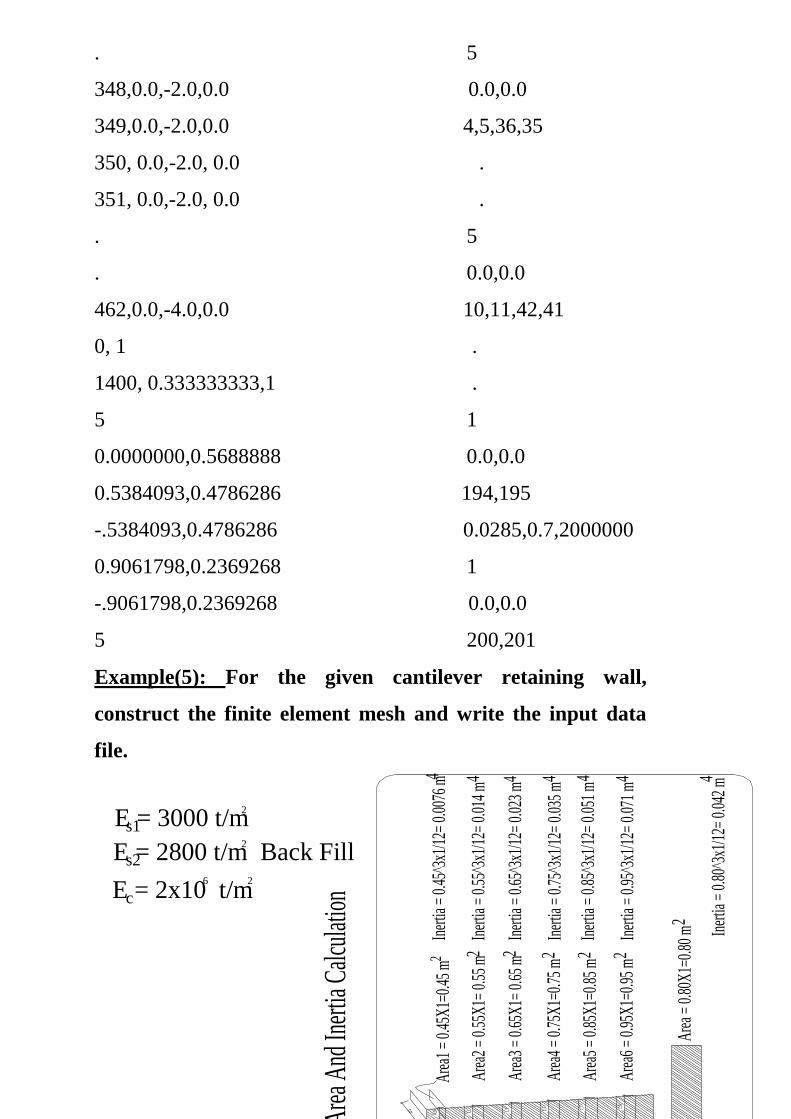
E = 2x10 t/m

E = 3000 t/m

c

s1

2

2

E = 2800 t/m Back Fills22

. 5

348,0.0,-2.0,0.0 0.0,0.0

349,0.0,-2.0,0.0 4,5,36,35

350, 0.0,-2.0, 0.0 .

351, 0.0,-2.0, 0.0 .

. 5

. 0.0,0.0

462,0.0,-4.0,0.0 10,11,42,41

0, 1 .

1400, 0.333333333,1 .

5 1

0.0000000,0.5688888 0.0,0.0

0.5384093,0.4786286 194,195

-.5384093,0.4786286 0.0285,0.7,2000000

0.9061798,0.2369268 1

-.9061798,0.2369268 0.0,0.0

5 200,201

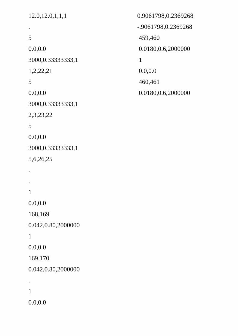
Example(5): For the given cantilever retaining wall,

construct the finite element mesh and write the input data

file.

1 1 1 1 1 1 1 1 1 1 1 2 2 3

6.0

t

24

102

22

81

21

1

21

222

20

61

413

9

21

161

141

121

101

3.0

t6

.0t

0,5

0,5

410

12

22

11

11

11

11

11

1

8

25

5

4

34

3

23

24

76

5

67

26

22

9

168

4.5

t3.0

t3

.0t

3.0

t3

.0t

1.3

27

4t

2.0

47

6t

1.0

t3

.0t

0.1

25

t

40

20

60

2t

1.8

t0

.8t

2t

2t

2t

2t

4t

3t

4t

246

2t

Suitable Elements:

- Beam Element 11

- Friction Element 5 " at the base of the R.W "

- 4NIQE 212

- Infinite Element 41

2Node 39

1Node 2

NN 246

NE 269

246,223 .

0.0,0.0,0,0,0 18.0,18.0,1,1,0

2.0,0.0,1,0,0 20.0,18.0,1,1,0

4.0,0.0,1,0,0 22.0,18.0,1,1,0

. 24.0,18.0,0,1,0

. 23

10.0,0.0,1,0,0 161,0.0,-3.0,0.0

11.0,0.0,1,0,0 162,0.0,-6.0,0.0

11.5,0.0,1,0,0 163,0.0,-6.0,0.0

0.0,3.0,0,1,0 164,0.0,-4.5,0.0

2.0,3.0,1,1,0 168,0.0,-3.0,0.0

4.0,3.0,1,1,0 169,0.0,-3.0,0.0

. 170,1.327,0.0,0.0

9.0,3.0,1,1,0 244,0.0,-4.0,0.0

10.0,3.0,1,1,0 245,0.0,-4.0,0.0

11.0,3.0,1,1,0 246,0.0,-4.0,0.0

11.5, 3.0,1,1,0 .

12.0, 3.0,1,1,0 .

. 1,0

. 5

10.0,12.0,1,1,1 0.0000000,0.5688888

11.0,12.0,1,1,1 0.5384093,0.4786286

11.5,12.0,1,1,1 -0.5384093,0.4786286

12.0,12.0,1,1,1 0.9061798,0.2369268

. -.9061798,0.2369268

5 459,460

0.0,0.0 0.0180,0.6,2000000

3000,0.33333333,1 1

1,2,22,21 0.0,0.0

5 460,461

0.0,0.0 0.0180,0.6,2000000

3000,0.33333333,1

2,3,23,22

5

0.0,0.0

3000,0.33333333,1

5,6,26,25

.

.

1

0.0,0.0

168,169

0.042,0.80,2000000

1

0.0,0.0

169,170

0.042,0.80,2000000

.

1

0.0,0.0