an interest rate model for counterparty credit risk - tu delft

Delft University of TechnologyFaculty of Electrical Engineering, Mathematics and Computer Science

Delft Institute of Applied Mathematics

An interest rate model for counterparty credit risk

A thesis submitted to theDelft Institute of Applied Mathematicsin partial fulfillment of the requirements

for the degree

MASTER OF SCIENCEin

APPLIED MATHEMATICS

by

M.C.A. de Ruijter

Delft, the NetherlandsMay 2010

Copyright c© 2010 by M.C.A. de Ruijter. All rights reserved.

MSc THESIS APPLIED MATHEMATICS

“An interest rate model for counterparty

credit risk”

M.C.A. de Ruijter

Delft University of Technology

Daily supervisors Responsible professor

Drs. J. Hommels (Rabobank) Prof. dr. F.M. Dekking

Dr. J.A.M. van der Weide (TU Delft)

Other thesis committee members

Prof. dr. C.W. Oosterlee

June 2010 Delft, the Netherlands

Abstract

Counterparty credit risk is one of the many types of risk a financial institution such as a bankhas to deal with. It is defined as the risk that the counterparty to a derivative transactioncould default before the final settlement of the transaction´s cash flows. Quantifying counter-party credit risk is complicated since the loss due to the default of a counterparty is uncertainfor a derivative contract. The future value of a derivative contract depends on one or severalmarket factors. To calculate the counterparty credit risk we estimate the exposure distribu-tion for each of the derivative contracts with a certain counterparty. This can amongst othersbe done by Monte Carlo simulation. It involves using Monte Carlo simulation to generate alarge number of possible future scenarios for several market factors. These scenarios will thenbe used to value every derivative contract, through time. This results in a exposure distribution.

Before we can generate these scenarios we have to develop a model for each of the marketfactors. In this thesis we will focus on the development of a model for the interest rates. We willresearch several options for the estimaton of the parameters such as maximum likelihood butalso methods based on the market expectations theory and the characteristics of the historicaldata. The model used here is a geometric Brownian motion with mean reversion process forthe forward rates. Using the historical data we will assess the fit of this model to the historicaldata. We will research options to change the parameter estimates in such a way that we willnot underestimate the counterparty credit risk. We will also research the assumptions madein the model. The performance of the model chosen will also be assessed by the calculation ofthe characteristics of the exposure distribution for two interest rate derivatives, the interest rateswap and the forward rate agreement.

iii

Preface

This is it, the report of my Master’s thesis at Rabobank International. Several months precededthis report, for which the foundation was laid in July 2009. During my studies, I got more andmore interested in the applications of mathematics in finance. After attending various courseson finance, Hans van der Weide pointed me on the opportunity to do an internship for my thesisat Rabobank International. From my curiosity in finance, it seemed to me as a great chance tosee how to apply mathematical principles in a business setting. More specifically, I have put mymathematical knowledge to use in the area of counterparty credit risk. A very interesting topic,where I learned a lot about in a very short period. Besides content-wise, the project exhibitedthe interesting company Rabobank International, great colleagues, and a challenging workingenvironment.

Therefore, I would like to first of all thank my supervisor at Rabobank International, JasperHommels. From the start of my internship, his support has enabled me to complete this thesiswork. In our meetings, he provided great input and together we cracked various challenges.Furthermore, I want to thank everybody I met during my internship at Rabobank for theirinterest in my work, especially everybody at the Quantative Risk Analytics deparment.

Without support from Delft University of Technology, I would not have been able to performthis project. First of all, thanks to Hans van der Weide for pointing out the opportunity of grad-uating at Rabobank International. It triggered me to make the first step towards performingthis thesis work. Michel Dekking and Kees Oosterlee, I want to thank you together with Hansfor reviewing this thesis report and my thesis defence.

Furthermore, I want to thank my family and friends, especially my boyfriend. Besides listeningto every issue I had when writing this thesis and all the enthusiastic stories about what I wasworking on, he was also a great help with some of the figures.

A final thanks goes to you, my reader. Thanks for your interest in this report and my thesiswork. This work considerably contributed to my knowledge on finance and counterparty creditrisk. Curious about what I learned? Please continue and have fun reading!

Marieke de RuijterAmsterdam, The Netherlands

June, 2010

v

Contents

List of Figures ix

List of Tables xi

List of Abbreviations xiii

1 Counterparty credit risk 1

1.1 Potential future exposure . . . . . . . . . . . . . . . . . . . . . . . . . . . . . . . 3

1.2 Exposure at default . . . . . . . . . . . . . . . . . . . . . . . . . . . . . . . . . . 5

1.3 Outline . . . . . . . . . . . . . . . . . . . . . . . . . . . . . . . . . . . . . . . . . 7

2 Interest rate products 9

2.1 Forward rate agreements . . . . . . . . . . . . . . . . . . . . . . . . . . . . . . . . 10

2.2 Interest rate swaps . . . . . . . . . . . . . . . . . . . . . . . . . . . . . . . . . . . 11

2.3 The historical exposure for the FRA and the IRS . . . . . . . . . . . . . . . . . . 13

3 Data analysis 17

3.1 Interest rate data . . . . . . . . . . . . . . . . . . . . . . . . . . . . . . . . . . . . 17

3.2 Forward rates . . . . . . . . . . . . . . . . . . . . . . . . . . . . . . . . . . . . . . 18

3.3 Yield curve . . . . . . . . . . . . . . . . . . . . . . . . . . . . . . . . . . . . . . . 20

4 Interest rate models 21

4.1 Requirements for the interest rate model . . . . . . . . . . . . . . . . . . . . . . . 21

4.2 Potential models for the interest rate . . . . . . . . . . . . . . . . . . . . . . . . . 22

4.3 Modeling forward rates . . . . . . . . . . . . . . . . . . . . . . . . . . . . . . . . . 24

4.4 Geometric Brownian motion with mean reversion . . . . . . . . . . . . . . . . . . 25

4.5 Correlation . . . . . . . . . . . . . . . . . . . . . . . . . . . . . . . . . . . . . . . 28

4.5.1 Proof of equation (4.28) . . . . . . . . . . . . . . . . . . . . . . . . . . . . 30

4.6 Disadvantage of the model . . . . . . . . . . . . . . . . . . . . . . . . . . . . . . . 31

5 Calibration 33

5.1 Estimation of the correlation ρ . . . . . . . . . . . . . . . . . . . . . . . . . . . . 33

5.2 The method of least squares/maximum likelihood estimation . . . . . . . . . . . 34

5.2.1 Independent estimation of σ . . . . . . . . . . . . . . . . . . . . . . . . . . 39

5.3 Market expectations theory . . . . . . . . . . . . . . . . . . . . . . . . . . . . . . 40

5.3.1 Disadvantages of this approach . . . . . . . . . . . . . . . . . . . . . . . . 42

5.3.2 Advantages of this approach . . . . . . . . . . . . . . . . . . . . . . . . . . 44

5.4 Using long term quantiles . . . . . . . . . . . . . . . . . . . . . . . . . . . . . . . 46

5.5 Comparison of methods . . . . . . . . . . . . . . . . . . . . . . . . . . . . . . . . 51

vii

viii CONTENTS

6 Residuals 57

6.1 Standard normal distributed residuals . . . . . . . . . . . . . . . . . . . . . . . . 576.1.1 Kurtosis scaling . . . . . . . . . . . . . . . . . . . . . . . . . . . . . . . . . 596.1.2 Quantile scaling . . . . . . . . . . . . . . . . . . . . . . . . . . . . . . . . 606.1.3 Comparison of scaling methods . . . . . . . . . . . . . . . . . . . . . . . . 61

6.2 Independent and identically distributed residuals . . . . . . . . . . . . . . . . . . 64

7 Conclusions 71

Bibliography 74

A Calculations method of least squares 77

B Calculations maximum likelihood method 79

C Value of the floating leg part in an IRS 81

List of Figures

1.1 Illustration of how to compute the PFE. . . . . . . . . . . . . . . . . . . . . . . . 4

1.2 Illustration of the computation of the effective EPE. . . . . . . . . . . . . . . . . 6

2.1 Notional outstanding per type of OTC derivative. . . . . . . . . . . . . . . . . . . 9

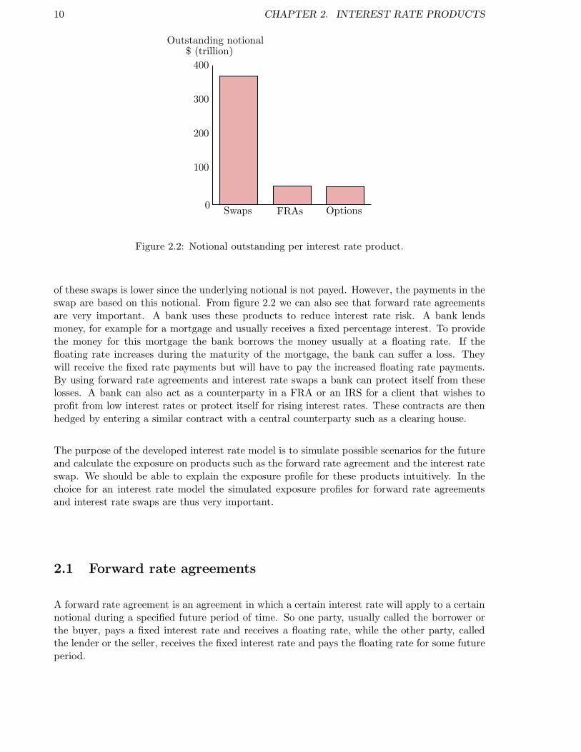
2.2 Notional outstanding per interest rate product. . . . . . . . . . . . . . . . . . . . 10

2.3 The exposure for a FRA starting at 26-04-2005. . . . . . . . . . . . . . . . . . . . 14

2.4 The exposure for a IRS starting at 20-12-2002. . . . . . . . . . . . . . . . . . . . 14

3.1 The 6 months and 20 years tenor points for the EUR interest rate data. . . . . . 18

3.2 The 6 months and 20 years tenor points for the USD interest rate data. . . . . . 18

3.3 The stepwise behavior of the 1 month EUR interest rate. . . . . . . . . . . . . . 19

3.4 The 6 months to 1 year forward rate, calculated from the interest rate data. . . . 19

3.5 Fitted yield curve at 3-12-2008 (black solid) and 2-12-2009 (green dashed). . . . . 20

4.1 A simulated path for the geometric Brownian motion with mean reversion model. 28

4.2 The correction factor c depending on the size of the time step ∆t. . . . . . . . . 30

4.3 The influence of the start value on the mean reversion. . . . . . . . . . . . . . . . 31

5.1 Density of bootstrapped estimators for k including the input value (red line). . . 36

5.2 Density of bootstrapped estimators for θ including the input value (red line). . . 36

5.3 Density of bootstrapped estimators for σ including the input value (red line). . . 37

5.4 Estimator for k through time using partitions of 1000 observations. . . . . . . . . 38

5.5 Estimator for θ through time using partitions of 1000 observations. . . . . . . . . 38

5.6 Estimator for σ through time using partitions of 1000 observations. . . . . . . . . 38

5.7 Implied expectations and the approximation by equation (5.15). . . . . . . . . . . 41

5.8 Estimates for k for the last 1000 days in the dataset. . . . . . . . . . . . . . . . . 43

5.9 Estimates for θ for the last 1000 days in the dataset. . . . . . . . . . . . . . . . . 43

5.10 The humped yield curve at 18-12-2008. . . . . . . . . . . . . . . . . . . . . . . . . 44

5.11 Approximation of the implied expectation of a humped yield curve. . . . . . . . . 44

5.12 The 2.5% and 97.5% quantiles of the simulated 5-10y forward rate. . . . . . . . . 45

5.13 The 2.5% and 97.5% quantiles of the simulated exposure for an FRA. . . . . . . 46

5.14 The 95% confidence interval for the 6 months to 1 year EUR forward rate. . . . . 49

5.15 The 95% confidence interval for the 0 to 1 month EUR forward rate. . . . . . . . 49

5.16 The 95% confidence interval for the 1 year EUR interest rate. . . . . . . . . . . . 50

5.17 The 95% confidence interval for the 20 years EUR interest rate. . . . . . . . . . . 50

5.18 The simulated PFE for an IRS where we pay floating and receive fixed. . . . . . 52

5.19 The simulated PFE for an IRS where we pay fixed and receive floating. . . . . . 52

5.20 The simulated PFE for an FRA where we pay floating and receive fixed. . . . . . 53

5.21 The simulated PFE for an FRA where we pay fixed and receive floating. . . . . . 54

ix

x LIST OF FIGURES

6.1 The density of the residuals for the USD 1y-2y forward rate. . . . . . . . . . . . 586.2 The density of the residuals R for the USD 1y-2y forward. . . . . . . . . . . . . . 596.3 The distribution of σεε for the different scaling methods. . . . . . . . . . . . . . . 626.4 The quantiles for an interest rate swap using different scaling methods. . . . . . . 636.5 The quantiles for the 6m-1y EUR forward rate using different scaling methods. . 636.6 Clustering in the EUR 10y-20y forward rate residuals. . . . . . . . . . . . . . . . 656.7 Autocorrelation function for the EUR 10y-20y forward rate residuals. . . . . . . . 656.8 Simulated quantiles for the 5 to 10 year forward rates. . . . . . . . . . . . . . . . 676.9 Simulated quantiles for the 5 to 10 year forward rates. . . . . . . . . . . . . . . . 686.10 Simulated quantiles for a 5 year interest rate swap. . . . . . . . . . . . . . . . . . 68

List of Tables

5.1 Estimates for k, θ and σ using the method of least squares/maximum likelihood 355.2 Estimates for σ. . . . . . . . . . . . . . . . . . . . . . . . . . . . . . . . . . . . . . 395.3 Estimates for k, θ and σ using market expectations theory. . . . . . . . . . . . . 415.4 Available long term interest rate data per tenor point. . . . . . . . . . . . . . . . 475.5 Quantiles and parameter estimates for the long term quantile method. . . . . . . 48

6.1 Kurtosis of the historical residuals and the resulting scaling for σ. . . . . . . . . . 606.2 Quantiles of the historical residuals and the resulting scaling for σ. . . . . . . . . 616.3 Parameter estimates for GARCH parameters. . . . . . . . . . . . . . . . . . . . . 666.4 Estimates for σt0 and the long term mean for σ. . . . . . . . . . . . . . . . . . . . 67

xi

xii LIST OF TABLES

List of Abbreviations

CCR counterparty credit risk

CRD Capital Requirements Directive

CSA credit support annex

DNB De Nederlandse Bank

EAD exposure at default

EE expected exposure

EPE expected positive exposure

FRA forward rate agreement

IRS interest rate swap

OTC over-the-counter

PFE potential future exposure

SFT security financing transaction

xiii

xiv LIST OF TABLES

Chapter 1

Counterparty credit risk

Financial institutions are subject to several types of risk such as credit risk and market risk.To safeguard themselves against these risks and to meet regulations these institutions have toquantify the risks they bear. One of these risks is counterparty credit risk, the risk that thecounterparty to a derivative transaction could default before the final settlement of the transac-tion’s cash flows1. Only over-the-counter (OTC) derivatives and security financing transactions(SFT) are subject to counterparty credit risk, since exchange-traded derivatives payments areguaranteed by the exchange. Counterparty credit risk is similar to other types of credit risk,for example the credit risk involved with a loan, since the cause of the loss is the default ofthe counterparty. Two distinctive features of counterparty credit risk are the uncertainty ofthe magnitude of the possible loss and the fact that both parties in a contract may face anexposure, which is the positive value of the contract assuming zero recovery in case of default.For a derivative contract the value depends on the future development of one or several marketfactors, such as interest rates. We can illustrate the bilateral nature of the risk by consideringan interest rate product with a certain counterparty, where for us the value of the contract willrise as interest rates rise. Then if interest rates rise the counterparty owes us money. However,if interest rates decrease the value of the contract will be negative for us, which means that weowe the counterparty money. So depending on the development of future interest rates bothparties can have an exposure.

Two examples of over-the-counter derivatives are interest rate swaps (IRS) and forward rateagreements (FRA). In an interest rate swap two parties agree to swap floating interest rate pay-ments for fixed interest rate payments based on a specified notional. In a forward rate agreementtwo parties agree to swap a floating interest rate payment for a fixed interest rate payment on aspecified notional for a single specified future period. Despite of the fact that in these contractsthe notional and fixed payments are agreed on, the future floating interest rate depends on thedevelopment of the interest rates and cannot be determined in advance. The value of an interestrate swap or a forward rate agreement will thus be uncertain for any time point in the future.The forward rate agreement and the interest rate swap will be discussed in detail in chapter2. Both the interest rate swap and the forward rate agreement fall in the category of interestrate derivatives. Besides interest rate derivatives also credit, equity, currency and commodityderivatives fall under over-the-counter derivatives and are subject to counterparty credit risk. Iffor example a financial institution has such a OTC-derivative contract with a certain counter-party and this counterparty defaults during the maturity of the contract there are two possiblescenarios. If the value of the contract is negative, meaning that the financial institution owesthis counterparty money, there will be no loss to the financial institution. This institution will

1Quoted from article 5:1 in DNB [7], documentation of the Dutch Central Bank.

1

2 CHAPTER 1. COUNTERPARTY CREDIT RISK

close out their position by paying the market value of the contract to the defaulting counterpartyand enter a similar contract with another counterparty where they will receive the market valueof the contract. If the value of the contract is positive, the financial institution will also closeout their position, making a claim equal to the positive value of the contract. Depending onthe recovery rate they may recover a part of the value of the contract. However, to enter asimilar contract with another counterparty the institution will have to pay the market value ofthe contract. The loss will thus be equal to the value of the contract less any recovery value.This means that only when the value of the contract is positive the financial institution willsuffer a credit loss in case of default of the counterparty.

Security lending transactions, repos and sell/buy back transactions are examples of securityfinancing transactions. These kind of transactions are also subject to counterparty credit risk.The common factor in these transactions is the temporary transfer of a security. In a securitylending transaction a security is temporarily lent by one party (the lender) to another party(the borrower) mostly on a collateralized basis. The borrower is obliged to return the secu-rities and will have to pay a certain fee for the lending. This lending is done to cover shortpositions for example. With a repo or sale and repurchase agreement one party (the seller)sells securities to another party (the buyer) where the parties agree that these securities will berepurchased at a specified date for a specified price. A sell/buy back transaction is similar to arepo but technically consists of two transactions; the selling of the securities and a simultaneousforward repurchase. The purpose of a repo or a sell/buy back transaction is either the transferof ownership of the security or to obtain a loan, generally at a lower rate then an unsecuredloan. The rate for this loan is lower since, in case of default of the seller the buyer still ownsthe securities. Just as with OTC derivatives the magnitude of the possible loss in case of de-fault is uncertain since this will depend on the value of the securities involved in the transaction2.

Also Rabobank will have to quantify their counterparty credit risk. To be compliant with themost risk sensitive measures for counterparty credit risk the Horizon project has been set up inRabobank. The goal of the project is two-fold. Firstly, Rabobank wants to be able to assess thepossible future exposure for every counterparty as accurately as possible to be confident that thefuture exposure for a counterparty does not exceed the limits set for this exposure. Secondly,Rabobank wants to be compliant with the most sophisticated regulations for capital reserves. Inthe Netherlands banks are regulated by the Dutch central bank (DNB). The Dutch regulationsfor counterparty credit risk are described in the Supervisory Regulation on Solvency Require-ments for Credit Risk see DNB [7]. These regulations are based on the Capital RequirementsDirective (CRD) which is meant to implement a supervisory framework for financial institutionsin the European Union.

The Horizon project consists of several steps. First, huge amounts of historical data for severalrisk drivers have to be collected and processed. Then models will have to be developed for therisk drivers. The Rabobank will then use Monte Carlo simulation to generate future scenariosfor these risk drivers. Using these scenarios the derivative contracts will be valuated, which iswhy the next step is to develop pricing functions for each of the derivative contracts. Withthese pricing functions we will obtain the value of several derivative contracts in all generatedscenarios. The last step in the project is then to process this data into a report based on whichseveral decisions about the counterparty credit risk can be made. During my internship atRabobank I cooperated on the development of models for the risk drivers, specifically on themodel for interest rates. The main purpose of this thesis is to develop an interest rate model

2More information about this kind of transactions can be found in Fabozzi and Mann [9].

1.1. POTENTIAL FUTURE EXPOSURE 3

for counterparty credit risk. This involves answering the following questions:

• How will the interest rate model be used to quantify counterparty credit risk?

• What interest rate products will be priced using this interest rate model?

• What kind of historical interest data do we have? How can we use this data?

• Which models are available for interest rates? What specific requirements do we have foran interest rate model for counterparty credit risk? Why do we choose a certain model?

• What are the characteristics of the chosen interest rate model? How do we simulate interestrates using this model?

• How can we incorporate correlation between interest rates at different maturities, interestrates of different currencies and other risk drivers?

• How do we calibrate the parameters in the chosen model?

• Which assumptions are made in the model? Are these assumptions reasonable using thehistorical data?

• What are the restrictions of the model used?

In this thesis we will try to answer all of these questions. In the rest of this chapter we willdescribe how the interest rate will be used to quantify counterparty credit risk and what measuresare available for this purpose. In section 1.1 the potential future exposure is defined. Thismeasure is used internally to be able to compare the possible future exposure to the limits setfor this exposure. We will describe the process used to quantify counterparty credit risk ingreat detail in this section. Section 1.2 will be used to explain how financial institutions shouldcompute their regulatory capital for counterparty credit risk. This involves a different measure,the exposure at default.

1.1 Potential future exposure

To quantify counterparty credit risk, the exposure per counterparty is calculated. The exposureper counterparty is defined as the maximum of zero and the market value of the portfolio ofderivative positions with this counterparty. This is the amount that would be lost due to defaultof the counterpary in case of zero recovery. Since the value of OTC-derivatives changes overtime due to market factors such as interest rates, only the current exposure can be calculatedwith certainty. The future exposure is uncertain. However large exposures would lead to largelosses in case of default of the counterpary, so a bank will set limits to the amount of exposureover time for every counterparty. One can assess the possible exposure for a certain time t in thefuture by calculating the exposure in several possible future scenarios for time t, where each ofthese scenarios corresponds to a possible set of market conditions. The exposure, computed foreach of these scenarios, will lead to a distribution of the potential exposure for the future time t.Using this distribution the potential future exposure (PFE) at time t is defined as a high, in thiscase 97.5% quantile of the exposure distribution. The PFE at time t is then the exposure thatwill only be exceeded with 2.5% probability. This quantity can be compared to the limits setfor the amount of exposure for a counterparty. Figure 1.1 illustrates the computation of the PFE.

In the Horizon project the Rabobank will implement Monte Carlo simulation to quantify expo-sure. Monte Carlo simulation is time consuming, depending on the number of counterparties,


Now Future dateHistory

PFE

Figure 1.1: Illustration of how to compute the PFE.

the number of transactions per counterparty and the number of scenarios generated, but is ableto capture the correlation between transactions and will as a consequence give a more accuratedistribution of the exposure compared to other methods. As described in Gregory [11] there areseveral methods to quantify exposure. The most simple method is an add-on method. Here theexposure is determined as the current exposure plus a component representing the uncertaintyin the exposure for the future. This add-on would ideally be different for every contract, ac-counting for the specifics of the transaction. However, for simplicity some of these specifics willbe ignored which can make the method inaccurate. A more complicated method is defining a(semi-)analytical expression for the exposure. By making assumptions about the market factors,one could approximate the potential future exposure analytically. Although an analytical ex-pression is easy to work with, the assumptions made will have to be over-simplifying to allow theexposure to be approximated analytically. Furthermore, using this method calculations throughtime are independent.

As mentioned above the calculation of the potential future exposure requires us to assess thedistribution of the exposure. Using Monte Carlo simulation we construct this distribution bygenerating a lot of scenarios corresponding to different market circumstances and calculate theexposure for every derivative at several future time points. To value, for example, a forward rateagreement we will have to model interest rates since the value of the forward rate agreementat a future date t depends on the interest rate at this time t. To calculate the potential futureexposure for several other transactions also foreign-exchange rates and credit spreads will bemodeled and simulated. To illustrate the calculation of the potential future exposure assumethat we have one contract with a certain counterparty. The value of this contract at a certaintime point t is given by V (t). The exposure E for this contract at some future time point t1 isthen given by

E(t1) = max(0, V (t1))

However the value of the contract at time t1 is unknown since the value changes due to changes

1.2. EXPOSURE AT DEFAULT 5

in the market. We assume that the value of this product depends on the interest rate. If weare able to model the interest rate we can, by simulating several scenarios of possible future in-terest rates calculate a range of possible future values for the contract V1(t1), . . . , Vn(t1). Usingthis values we can calculate the exposure in every scenario leading to a set of possible futureexposures E1(t1), . . . , En(t1). The potential future exposure is then given by the 97.5% quantileof the empirical distribution of possible exposures. When we assume that there is more thanone contract with a certain counterparty the potential future exposure for this counterparty isgiven by the sum of potential exposures per contract. The parties in a derivative contract canreduce their counterparty credit risk by means of a ISDA3 master agreement. In this agreementthe parties can decide on a netting agreement. In case of a netting agreement the value of allcontracts with this counterparty in a netting set are netted. In this case the exposure of a setof contracts is only the net positive value. An option in the ISDA master agreement is thecredit support annex (CSA). In case of a CSA one or both of the counterparties to a contractare required to pay collateral when the exposure exceeds some pre-specified threshold. Thiscollateral will reduce the exposure below the threshold. More on this approach can be found inZhu and Pykhtin [16].

1.2 Exposure at default

The regulation of banks on an international level started in 1974 following the collapse of theHerstatt Bank in Germany and the Franklin National Bank in the US due to amongst otherthings, bad international supervision. To improve international supervision the Basel Commit-tee on Banking Supervision was created. Their work led to the introduction of the Basel CapitalAccord in 1988, a framework for credit risk measurement. The current regulations are based ona revision of this capital accord, referred to as Basel II. The Basel II supervisory framework isimplemented in Europe through the CRD. The purpose of these regulations is to ensure thatevery bank holds capital reserves appropriate to the risk the bank is exposed to. This shouldstabilize the banking system and guarantee that banks have a sound risk management. The cap-ital reserves based on these regulations are usually referred to as regulatory capital. Recently,the Basel Committee on Banking Supervision has published a number of proposals to reformthe international supervisory framework as a result of the latest/current financial crisis. Oneof these proposals, which can be found in Basel [3] is to strengthen CCR capital requirements,since the financial crisis has shown that the current regulatory capital treatment for CCR is in-sufficient. This proposal may eventually lead to changes or additions to the Basel II framework.Since these changes have not been implemented so far we will in this thesis focus on the currentregulations.

The current regulations for credit risk include four methods for computing counterparty creditrisk, see DNB [7]. These methods are:

• Original exposure method

• Mark-to-market method (current exposure method)

• Standardized method

• Internal model method (IMM)

3ISDA stands for International Swaps and Derivatives Association. This organization has created the masteragreement, which is a standardized contract for derivative transactions.


Each of the subsequent methods is more risk sensitive than the previous but also more complex.The basic idea of these methods is to compute the loan equivalent exposure at default (EAD).A financial institution is supposed to choose a method that is appropriate for the nature andsize of their exposures. The original exposure method, which is the least risk sensitive method,may only be applied by institutions that fall under the ”des minimis” regulation. The internalmodel method, which is the most sophisticated method is subject to prior approval of the DutchCentral bank. With the Horizon project the Rabobank aims at implementing this method. Inthe internal model method the exposure at default will be computed using a model that specifiesa forecasting distribution for market variables such as interest rates. The exposure is then com-puted for a contract at a future date using the changes in the market variables. The frameworkdescribed for computing the potential future exposure in the previous section is similar to theframework needed to compute the EAD using the internal model method.

Effective EE

Exposure

Time

Effective EPE

EPE

EE

Figure 1.2: Illustration of the computation of the effective EPE.

Using the internal model method one will have to determine the loan equivalent exposure atdefault for every counterparty. The exposure at default is used to calculate the required capitalreserves. The actual exposure at default is a random exposure. We do not know the exposureat default unless we know when the counterparty will default. To simplify calculations we willuse the loan equivalent exposure at default which involves calculating a fixed exposure, allowingderivative positions to be treated similar to the more simple loans. The most natural choice forthis fixed exposure is the expected positive exposure (EPE). This is a loan equivalent measuresince the expected loss for the counterparty will in this case be equal for both random and fixedexposures. The exposure at default is then given by

EAD = α · Effective EPE

To obtain the EAD, we multiply the effective EPE by a constant factor α, which will amongstothers account for the correlation between exposures and defaults. For the internal modelmethod the value of α is set at a level of 1.4. However, a financial institution can obtain approvalto compute their own estimate for α subject to a floor of 1.2. If we use the models for marketvariables to simulate future scenarios and value the contracts with a certain counterparty in eachof these scenarios we have an exposure distribution. Using this distribution we can estimate theexpected exposure (EE) at any future time t as the average over the exposure in every scenario

1.3. OUTLINE 7

for time t. As a function of time the expected exposure will initially increase but from the pointwhere the maturity is reached the exposure will be equal to zero. It is however likely that thebank will enter new transactions in the future. This will result in roll-over risk, the additionalexposure generated by future financial transactions. To account for the roll-over risk we will usethe effective EE which will be a monotonically increasing function of t since it is defined by

Effective EE(t) = max(EE(t− 1), EE(t))

The average of the effective EE over time is then denoted as the effective expected positiveexposure, needed to compute the exposure at default. Figure 1.2 illustrates how the effectiveEPE is computed.

1.3 Outline

In the introduction we have explained the main purpose of this thesis: the development of aninterest rate model. We aim to answer the questions in this chapter. In this chapter we havealready explained how counterparty credit risk is quantified and why we need an interest ratemodel. We have also described the use of the model: simulating future scenarios for the interestrates. These scenarios will then be used to value derivatives. In chapter 2 we will describe twoof the most important OTC derivatives, the interest rate swap and the forward rate agreement.We will explain how these products are valued. Though the thesis we will use these products toassess the performance of the model.

The next step in the development of an interest rate model is analyzing the available data. Wewant to use this data to calibrate the parameters in the model but also to assess the fit of themodel. In the Horizon project the interest rate model will be used for interest rates for differentcurrencies. In this thesis we will only consider EUR and USD interest rates. We will limit theanalysis of the historical data to the historical interest rates for these two currencies.

Then we will choose one of the many available interest rate models in chapter 4. This chapterwill start by stating the specific requirements for the interest rate model for counterparty creditrisk. Then we will describe and compare several well known models. We will explain the choicefor the final model used and we will describe exactly how this model is defined and how we cansimulate interest rates using this model. We will also consider how correlation between interestrates at different maturities can be incorporated into the model.

After the model is selected, we have to estimate the parameters. In chapter 5 we will firstdescribe how the correlation is estimated. Then we will estimate the other parameters basedon the historical data using several methods. Each of these methods has both advantages anddisadvantages. We will use the interest rate swap and the forward rate agreement to assess theperformance of these methods for parameter estimation. We will choose one of these methods.This method will be used in the rest of the thesis.

The historical data has been used for the estimation of the parameters but can also be used toassess certain assumptions made in the interest rate model. In chapter 6 we will show whetherthe model is suitable for the historical data. We will test the assumption that the residualsin the model are standard normal distributed and that these residuals are independent. Wepropose some practical alternatives and assess the results of these alternatives by consideringthe impact on the potential future exposure for the interest rate swap.


Finally, we will conclude this thesis in chapter 7 by summarizing the results of the assessmentof the model and making some general comments on the use of the model.

Chapter 2

Interest rate products

In chapter 1 we have described how counterparty credit risk can be quantified. The scenariosgenerated using the interest rate models will be used to calculate the potential future exposureor the exposure at default for several derivative products depending on interest rates, interestrate derivatives. To be able to assess the model adequately we have to consider the exposure forsome important interest rate products. For this reason we will describe two basic but importantinterest rate products in this chapter. Interest rate products account for the biggest part of thetotal outstanding notional of OTC derivatives as can be seen in figure 2.1. The first productconsidered is the forward rate agreement (FRA). With this agreement an interest rate specifiedin the contract will apply to a specified notional value for a specified future period of time. Thesecond product we consider is the interest rate swap (IRS). In an interest rate swap two partiesagree to swap at specified future dates floating rate payments for fixed rate payments based onan agreed notional. In figure 2.2 we can see that the major part of the outstanding notional ininterest rates products is due to interest rate swaps1. Note however that the total market value

Interest rate

Foreign exchange

CDS

$ (trillion)

0

100

200

300

400

Outstanding notional

500

Commodity

OtherEquity linked

Figure 2.1: Notional outstanding per type of OTC derivative.

1The data for these figures is from BIS [2]

9

10 CHAPTER 2. INTEREST RATE PRODUCTS

Swaps FRAs Options

$ (trillion)

0

100

200

300

400

Outstanding notional

Figure 2.2: Notional outstanding per interest rate product.

of these swaps is lower since the underlying notional is not payed. However, the payments in theswap are based on this notional. From figure 2.2 we can also see that forward rate agreementsare very important. A bank uses these products to reduce interest rate risk. A bank lendsmoney, for example for a mortgage and usually receives a fixed percentage interest. To providethe money for this mortgage the bank borrows the money usually at a floating rate. If thefloating rate increases during the maturity of the mortgage, the bank can suffer a loss. Theywill receive the fixed rate payments but will have to pay the increased floating rate payments.By using forward rate agreements and interest rate swaps a bank can protect itself from theselosses. A bank can also act as a counterparty in a FRA or an IRS for a client that wishes toprofit from low interest rates or protect itself for rising interest rates. These contracts are thenhedged by entering a similar contract with a central counterparty such as a clearing house.

The purpose of the developed interest rate model is to simulate possible scenarios for the futureand calculate the exposure on products such as the forward rate agreement and the interest rateswap. We should be able to explain the exposure profile for these products intuitively. In thechoice for an interest rate model the simulated exposure profiles for forward rate agreementsand interest rate swaps are thus very important.

2.1 Forward rate agreements

A forward rate agreement is an agreement in which a certain interest rate will apply to a certainnotional during a specified future period of time. So one party, usually called the borrower orthe buyer, pays a fixed interest rate and receives a floating rate, while the other party, calledthe lender or the seller, receives the fixed interest rate and pays the floating rate for some futureperiod.

2.2. INTEREST RATE SWAPS 11

We will use the following notation in the definition of the FRA:

N = notional underlying the contractrfix = fixed interest rate agreed on in the contractT0 = starting date of the contractT1 = effective date, which is the first day of the agreed FRA− periodT2 = termination date, which is the last day of the agreed FRA− period

At the termination date of the contract one would receive (or pay) the difference between thefloating rate and the fixed rate for the period T2 − T1 for the notional N . Here we assume thatthe period between the effective date T1 and the termination date T2 is less than a year. Thisperiod is usually 3 or 6 months. The cashflow at time T2 would then be given by

C = N(

er(T1;T1,T2)(T2−T1) − 1− rfix · (T2 − T1))

(2.1)

However we assume2 here that the forward rate agreement is settled at the effective date T1. Atthis point the actual interest rate used for the FRA-period is known. Because of this settlement,the actual cashflow as a result of the contract will be at T1. To obtain this cashflow we discount(2.1) from time T2 to T1. If we pay fixed and receive the floating rate payment the cashflow isequal to

V (T1) = Ce−r(T1;T1,T2)(T2−T1) (2.2)

Furthermore, we assume that the fixed rate in the contract is chosen in such a way that thevalue of the contract is zero at T0: V (T0) = 0. Since the FRA is settled at T1 the value will onlydiffer from zero in the interval [T0, T1]. To determine the value of the FRA at a time point t inthis interval we need an estimate for the interest rate at time T1 with maturity T2 − T1. We usethe forward rate for the period [T1, T2] at t. Furthermore, we have to discount with the interestrate at t with maturity T2 denoted by r(t; t, T2) . The value of a FRA in the interval [T0, T1] isthen given by

V (t) =

0 t = T0

Ce−r(t;T1,T2)(T2−t) t ∈ (T0, T1)

Ce−r(T1;T1,T2)(T2−T1) t = T1

0 t > T1

(2.3)

As mentioned in the introduction the exposure of a single contract is given by maximum ofthe value of the contract and zero. If we want to calculate the potential future exposure fora forward rate agreement, we simulate a huge number of interest rate scenarios and value theforward rate agreement in each of these scenarios through time. The potential future exposureat time t is then given by the 97.5% quantile of the range of values of the forward rate agreementin every interest rate scenario at time t. Because of the settlement at time T1 the exposure canonly be positive in the interval [0, T1].

2.2 Interest rate swaps

An interest rate swap is an interest rate derivative where one party swaps their interest ratepayments with the interest rate payments of the other party. In most cases floating interestrate payments are swapped for fixed interest rate payments or vice versa. In this product thereis a maturity M, a number of fixed rate payments n1 and a number of floating rate paymentsn2. Furthermore the parties have agreed on a fixed interest rate and the notional N where the

2This assumption is common, see page 85 in Hull [12]: Usually FRAs are settled at time T1 rather than T2.


payments are based on. In different currencies the number of payments may differ, for examplefor EUR interest rate swaps it is convention that the fixed rate payments occur every year andthe floating payments every six months. For USD interest rate swaps it is convention that fixedpayments occur every 6 months and floating payments every three months.

There are several ways to value an interest rate swap. One might have seen the analogy betweenan interest rate swap with only one payment and the forward rate agreement described above.An interest rate swap can be seen as a portfolio of forward rate agreements payed in arrears.Another way to valuate an interest rate swap is by regarding the swap as a long position in onebond combined with a short position in another bond. We describe this method to value theinterest rate swap. We assume that the notional is exchanged at the maturity of the contract,which justifies this approach. However, since both parties pay the notional at the maturity ofthe contract, this leads to a payment with a net value of zero. We can define these two bondshere using the following notation:

Bfix = value of a fixed rate bond underlying the swapBfl = value of a floating rate bond underlying the swapN = notional principal underlying the swapti = time until ith payment is exchangedr(t; t, ti) = interest rate corresponding to maturity tirfix = fixed interest rate agreed on in the contractk = fixed payment made on the payment datesk∗ = floating payment made on the payment dates

Note that k is a payment fixed during the contract while k∗ is different for every payment,depending on the floating rate for the payment at hand. The value of the interest rate swapwhen fixed payments are received and floating payments are paid at time t, is given by

V (t) = Bfix(t)−Bfl(t) (2.4)

For an interest rate swap where one pays the fixed leg and receives the floating leg the valueof the interest rate swap is exactly the opposite: V (t) = Bfl(t) − Bfix(t). The value of thefixed-rate bond underlying the swap is given by the sum of the discounted fixed-payments andthe discounted notional:

Bfix(t) =

n1∑

i=1

1{t>ti}ke−r(t;t,ti)ti +Ne−r(t;t,tn)tn (2.5)

where n1 is the total number of fixed-payments. Using the fixed rate one can calculate the fixedpayments k. If there are m1 fixed rate payment per year, k is given by

k = N · rfix ·1

m1(2.6)

The value of the floating-rate bond is equal to a newly issued floating-rate bond after eachpayment. This is explained by an example in appendix C. Right after a payment the floating-ratepayment is known so the value of this floating-rate bond is equal to the discounted floating-ratepayment. The value of the floating-rate bond at a given day t is

Bfl(t) = (N + k∗)e−r(t;t,ti)ti (2.7)

Here i is the first payment after time t such that ti is the time until the next payment andr(t; t, t1) the interest rate corresponding to this maturity. We assume that the floating rate is

2.3. THE HISTORICAL EXPOSURE FOR THE FRA AND THE IRS 13

continuously compounding so, given m2 floating payments per year k∗ is given by

k∗ = N

(

exp

(

rfl ·1

m2

)

− 1

)

(2.8)

Here rfl is the floating rate set at the moment that the previous floating payment is due. Thismeans that at every moment the next floating payment is known. We assume that the fixedrate agreed on in the interest rate swap contract is chosen in such a way that the initial valueof the contract is 0.

By describing the interest rate swap we can already get an idea of the exposure of an interestrate swap. At t = 0 the exposure is zero. From this point the exposure will increase until thefirst payment. With every payment the exposure will decrease since part of the value of thecontract is already payed. At the maturity of the contract the value will have decreased to zeroagain.

2.3 The historical exposure for the FRA and the IRS

Using the historical data we can show the exposure of a forward rate agreement and an interestrate swap through time. This will give an idea of what the exposure can look like. For theforward rate agreement we start the contract at 26-04-2005 and take t = 0 at this date. Thestarting date of the FRA-period will be exactly one year later so T1 = 1. The termination dateof the contract will be 3 months after T1 so we have T2 = 1.25. We assume for simplicity thatN = 1. The fixed rate is chosen in such a way that the value of the contract is zero at the startdate of the contract t = 0. This means that the fixed rate in the contract is given by

rfix =er(0;T1,T2)(T2−T1) − 1

T2 − T1(2.9)

We assume that in this contract the fixed rate is payed and the floating rate is received. Infigure 2.3 we can see the value of this FRA given by the red dashed line. Where the valueof the FRA is positive this is equal to the exposure at that time. The exposure is given bythe blue line. We can see that the exposure is zero at t = 0 and then decreases initially. Fromt = 50 the value of the contract increases. At T1 the exposure drops to zero since the FRA is set-tled at this time. In the interval [T1, T2] the exposure is zero since the contract is already settled.

For the interest rate swap we will start the contract at 20-12-2002. The maturity of this contractwill be 5 years with annual payments for both the fixed and the floating leg. We assume that inthis contract we will pay floating and receive fixed. As in the FRA contract we choose the fixedrate in such a way that the value of the contract is zero at the start date of the contract. Thismeans that we have Bfix = Bfl which results in:

rfix =1− e−r(0;0,tn)tn

1m2

∑n1

i=1 e−r(0;0,ti)ti

(2.10)

From the red dashed line representing the value of the IRS in figure 2.4 we see that the value ofthe IRS is initially increasing. After about 240 days the value of the swaps decreases. The valueis negative from about 500 days after the start of the contract. At the termination date of thecontract the last payment is due which reduces the value of the interest rate swap to zero. The


0 50 100 150 200 250 300−1.5

−1

−0.5

0

0.5

1

1.5

2

2.5

3

3.5x 10

−3

Time (days)

Figure 2.3: The exposure for a FRA starting at 26-04-2005.

0 200 400 600 800 1000 1200−0.03

−0.02

−0.01

0

0.01

0.02

0.03

0.04

0.05

0.06

Time (days)

3rdpayment

2ndpayment

1stpayment 4th

payment

5thpayment

Figure 2.4: The exposure for a IRS starting at 20-12-2002.

2.3. THE HISTORICAL EXPOSURE FOR THE FRA AND THE IRS 15

black vertical lines in this figure indicate the times at which payments are due. Note that asthe contract is maturing the value curve is less spiky. This is caused by the fact that after eachpayment there is one insecure factor removed from the price. The value between the last twopayments is almost constant. This is because right after the fourth payment is due the floatingrate for the last payment is known, reducing the insecurity in the pricing. In future chapterswe will use the exposure profiles of forward rate agreements and interest rate swaps to assess,for example, the estimates for the parameters in the process. The exposure for this interest rateswap is given by the blue line.

Chapter 3

Data analysis

In the calibration and testing of the model historical interest rate data will be used. It isimportant to analyze this data first to get an idea of the data that is available and how it canbe used in the derivation of the model. The interest rate model should also be suitable for thehistorical data. Since in this thesis we will only look at the model for Euro and United Statesdollar interest rates, we require historical interest rates for both of these currencies. The dataarchive used by Rabobank contains daily interest rate data for these currencies from 22-01-2001until 01-12-2009, which is about 9 years of data. Interest rates are not the same for everymaturity. Generally the interest rate for a maturity of 30 years will be higher than the interestrate for a maturity of 1 month. To capture this relation between maturity and interest ratethrough time, the dataset contains information for 9 maturities. These maturities are calledtenor points and will be denoted by τ . The available tenor points for the interest rates are 1month, 3 months, 6 months, 1 year, 2 years, 5 years, 10 years, 20 years and 30 years. For thetenor points corresponding to a maturity less than or equal to 1 year the rates are given bythe interbank rate for this maturity. For tenor points corresponding to maturities longer than1 year the data corresponds to the swap rate for this maturity. The dataset consists of 2313data points for each of the nine maturities. In this thesis we assume that a year is 250 businessdays, excluding weekends and holidays. Since there was a change in the type of interest ratedata recorded after day 2038 in the dataset, resulting in a large jump from day 2038 to 2039 wehave shifted the data to remove these large jumps.

3.1 Interest rate data

In this section we will analyze the dataset in order to detect outliers or specific periods in theinterest rate data. These interest rates are continuous compounding rates. For all tenor pointsthe interest rates vary between 0.1% and 7.6%. For most of the history given, the interestrates corresponding to longer maturities such as 20 or 30 year are higher than the interest ratescorresponding to shorter maturities like 1 or 3 months. There is however a period in whichall interest rates are rather high with only small differences between the interest rates for dif-ferent tenor points. This period is followed by relatively low interest rates especially for theshort maturities. For the EUR interest rates this period corresponds to late 2007 to early 2009.For the USD interest rate this period is slightly earlier, starting in 2006 continuing through2007. These periods are due to the recent financial crisis, which started in 2006 in the UnitedStates and around 2007 in Europe. Figure 3.1 shows the 6 months and 20 years tenor pointsfor the EUR interest rates. In figure 3.2 one can see these tenorpoints for the USD interest rates.

Another notable aspect of the dataset is the stepwise change in several of the short maturity

17

18 CHAPTER 3. DATA ANALYSIS

0 500 1000 1500 20000

0.01

0.02

0.03

0.04

0.05

0.06

0.07

Time (days)

6m IR

20y IR

Figure 3.1: The 6 months and 20 years tenor points for the EUR interest rate data.

0 500 1000 1500 20000

0.01

0.02

0.03

0.04

0.05

0.06

0.07

Time (days)

6m IR

20y IR

Figure 3.2: The 6 months and 20 years tenor points for the USD interest rate data.

interest rates. This stepwise behavior is most obvious in the 1 month EUR interest rate, whichcan be seen in figure 3.3. The stepwise behavior of this interest rate is caused by the sensitivityof these short maturity interest rates to the policy of the central banks.

3.2 Forward rates

Forward rates are rates of interest implied by the current interest rates for a period of timein the future. For the pricing of interest rate products not only interest rates are used butalso forward rates. For example, in a forward rate agreement where we pay fixed and receivefloating rate for a period of 3 months starting 9 months from now the forward rate from 9 to12 months is chosen for the fixed rate to guarantee that the value of the contract is zero at thecontract date. Since the forward rate at time t is actually the interest rate for a future period oftime [T1, T2] we will denote the T1, T2-forward rate by r(t;T1, T2). This implies that the inter-

3.2. FORWARD RATES 19

0 500 1000 1500 20000

0.01

0.02

0.03

0.04

0.05

0.06

0.07

Time (days)

Figure 3.3: The stepwise behavior of the 1 month EUR interest rate.

0 500 1000 1500 20000

0.005

0.01

0.015

0.02

0.025

0.03

0.035

0.04

0.045

Time (days)

Figure 3.4: The 6 months to 1 year forward rate, calculated from the interest rate data.

est rate at time t for a maturity T will be denoted by r(t; t, T ). All times will be denoted in years.

If we consider the current interest rates for a maturity T1 and T2 where T2 > T1, the T1, T2-forward rate will be defined in such a way that there is no arbitrage possible. If 1 euro would beinvested at this moment for T2 years one would receive exp(r(0; 0, T2) · T2) after T2 years. Thisamount should be equal to the amount received when we first invest 1 euro for T1 years andthen reinvest for the period [T1, T2] for the current forward rate in this period: exp(r(0; 0, T1) ·T1) exp(r(0;T1, T2) · (T2 − T1)). If we solve this we find that the forward rate at time 0 for theperiod [T1, T2] is given by1

r(0;T1, T2) =r(0; 0, T2) · T2 − r(0; 0, T1) · T1

T2 − T1(3.1)

Using the relation given above we can compute the forward rates from the interest rate data.Figure 3.4 shows the 6 months to 1 year EUR forward rate through time. At every time point t

1This definition of the forward rate is also used in Hull [12].

20 CHAPTER 3. DATA ANALYSIS

0 5 10 15 20 25 300

0.01

0.02

0.03

0.04

0.05

0.06

Maturity (years)

Figure 3.5: Fitted yield curve at 3-12-2008 (black solid) and 2-12-2009 (green dashed).

this is the forward rate for the period 6 months to 1 year from t, implied in the interest rates attime t. We see in this figure that the behavior of the forward rate through time is very similarto the behavior of the interest rates.

3.3 Yield curve

The yield curve is the curve that represents the relation between the interest rate and the cor-responding maturity. Since the dataset used here consists of interest rates for several maturitieswe can construct the yield curve. The yield curve is most often2 upward sloping but in cases ofuncertainty or decline in the economy and in cases of deflation the shape of the yield curve canbe flat or negatively sloped. The upward sloping yield curve can be explained by the liquidity

preference theory. This is a theory from economics in which one assumes that the long-terminterest rates include a premium for the added risk of having the money fixed for a longer periodof time. This results in higher interest rates for long-term maturities.

Another theory motivating the shape of the yield curve is the market expectations hypothesis.With this hypothesis one assumes that the shape of the yield curve represents the expectationof the market participants for the future interest rates. Here an upward sloping yield curveis explained by the expectation that interest rates will rise in the future. If we for exampleassume that T1 and T2 are two maturities with T1 < T2 then the current forward rate from T1 toT2 implied in the yield curve is equal to the expected interest rate for the maturity T2−T1 at T1.

In figure 3.5 one can see the yield curve for two dates in the dataset for EUR interest rates.The black dots indicate the interest rates observed at 3-12-2008. The black line is a line fittedthrough these observations using cubic splines. This line is humped and does not have thetypical upward sloping shape. This could be explained by the uncertainty in the economy atthis time. The green dots indicate the interest rates observed at the last observation in the dataset, 2-12-2009. The green line is fitted through these dots using cubic splines. Here we see thetypical shape of the yield curve, although the 30 years tenor point is slightly lower than the 20years tenor point.

2See section 4.10 Theories of the term structure of interest rates in Hull [12].

Chapter 4

Interest rate models

As described earlier we need a model for the interest rates to be able to simulate interest ratescenarios for the future and determine the exposure profiles for products depending on theinterest rates. Using this profiles we will be able to calculate the potential future exposure for acounterparty. In the previous chapters we have described several of these interest rate productsand analyzed the historical data that will be used in the parameter estimation. In this chapterwe will describe the selection of the interest rate model and motivate the choice for the modelthat we will focus on in this thesis. The Horizon project and also the research on suitableinterest rate models started before my internship at Rabobank. A description of the research isincluded to give the reader a complete overview of the process and motivation for this model.We will conclude this chapter with a detailed description of the chosen interest rate model.

4.1 Requirements for the interest rate model

Modeling interest rates is very complex. To know exactly what the interest rates will be in thefuture one should know all factors that influence the interest rate and be able to estimate thesefactors. Since this is seen as an impossible job several stochastic models have been developedfor the interest rates. A large number of these models are described in Brigo and Mercurio[4]. Each of these models has both advantages and disadvantages. To choose between differentmodels we will have to keep the purpose of the model in mind. In this section we will list severalrequirements for the interest rate model.

• The model is required to simulate sensible interest rates. We require that both the interestrates and the forward rates are positive. Furthermore, the model must be suitable for thesimulation of interest rates for different currencies. To limit the extent of this thesis wewill only consider the two most important currencies for Rabobank, the Euro (EUR) andthe United States dollar (USD). Forward rates should be positive since these rates are usedin a interest rates swap or forward rate agreement as estimate for future interest rates.

• The model is required to be implementable without complex numerical approximation.Most of the models in Brigo and Mercurio [4] are described by a stochastic differentialequation. If this stochastic differential equation cannot be solved analytically we will haveto use numerical approximation techniques. However, with this numerical approximationwe will make a small error every step. For this reason it is preferable that the stochasticdifferential equation defining the model is analytically solvable. This allows us to simulatescenarios fast and efficient. The resulting (long term) behavior of the interest rates willbe transparent.

21

22 CHAPTER 4. INTEREST RATE MODELS

• The parameters in the model are required to be calibrated with the historical data available.These parameters should be reasonable and stable with respect to small changes in thedata.

• The model should allow for the definition of a clear correlation structure between interestrates at different maturities, interest rates in different currencies and other risk drivers.

• The model must generate reasonable exposure profiles for the derivatives (for example theinterest rate swap and the forward rate agreement).

• The model should be able to simulate interest rates using time steps of varying sizes.This is because the exposure exists for the maturity of a contract, which can be up to 30years. We would therefore want to compute the potential future exposure daily for thenext month but also in 10 years. It would however be very time consuming to simulateten years ahead using daily steps.

• The model should be used and accepted in the industry.

4.2 Potential models for the interest rate

In chapter 1 we have described the purpose of the interest rate model. We will use simulatedinterest rates to calculate prices for amongst others the interest rate swap through time. Tocalculate these prices while the contract is maturing, we will need simulated interest rates atevery maturity. For example, to value an interest rate swap we need to discount all fixed ratepayments using interest rates corresponding to the time to the payments. The simulation ofinterest rates at different maturities can be done in various ways. Firstly, we could simulatethe interest rates at several industry standard maturities. These standard maturities are, forexample the maturities in the historical dataset. A second option is to simulate the yield curveor properties of this yield curve through time. Although modeling the entire yield curve throughtime would give us the opportunity to calculate the interest rate at every maturity, we only havehistorical interest rate data available at 9 industry standard tenor points. The interest rateswill be modeled at these tenor points. Furthermore, it is chosen that one model will be used forall tenor points and all currencies. Per tenor point the parameters in the model will be calibrated.

The simplest models tested are Brownian motion models. Here we use the term Brownianmotion models for a group of models based on Brownian motion. The models in this group aredefined by the following general stochastic differential equation:

dr(t) = (b+ ar(t))dt+ σdW (t) + ξdJ(λ) (4.1)

Here b, a and σ > 0 are constants, W (t) is the Wiener process, ξ is a jump either random orconstant and J(λ) is a Poisson process with parameter λ. The Wiener process, the Poissonprocess and the jump ξ are assumed to be independent. The models in this group are:

• Simple Brownian motion (a = 0, b = 0, ξ = 0)

• Brownian motion with drift (a = 0, b 6= 0, ξ = 0)

• Brownian motion with mean reversion (a 6= 0, b 6= 0, ξ = 0) also known as the Vasicekmodel

• Brownian motion with mean reversion and jumps (a 6= 0, b 6= 0, ξ 6= 0), see Das [6]

4.2. POTENTIAL MODELS FOR THE INTEREST RATE 23

The main disadvantage of these models is the possibility to generate negative interest rates.Furthermore, the estimation of the parameters in the Brownian motion with mean reversionand jumps is very complicated. For these reasons all of these models are considered unsuitable.

The next group of models researched are geometric Brownian motion (GBM) models. Thesemodels are in a way the exponential versions of the Brownian motion models above. Themodels have the advantage that the simulated interest rates are always positive. The geometricBrownian motion models are:

• Simple geometric Brownian motion defined by dr(t) = σr(t)dW (t)

• Geometric Brownian motion with drift defined by dr(t) = µr(t)dt+ σr(t)dW (t)

• Geometric Brownian motion with mean reversion given by d ln(r(t)) = k (θ − ln(r(t))) dt+σdW (t)1

• Geometric Brownian motion with mean reversion and jumps given by d ln(r(t)) =k (θ − ln(r(t))) dt+ σdW (t) + ξdJ(λ)

In the stochastic differential equations above σ > 0, µ, k > 0, θ and λ are assumed to beconstant. W (t) is the Wiener process, ξ is a random or constant jump and J(λ) is a Poissonprocess. Again the Wiener process, the Poisson process and the jump ξ are assumed to be inde-pendent. Again the option with jumps was considered too complex because there is no analyticalsolution to the differential equation and the estimation of the parameters is very complicated.Furthermore using this option, determining a correlation structure is too complicated or notfeasible since we have to deal with two random processes. The other models in this group arerejected since it is possible to generate interest rates that will lead to negative forward rates.When pricing an interest rate swap or a forward rate agreement we will use these forward rates.Negative forward rates are considered unrealistic. Furthermore, the simple GBM model and theGBM model with drift are unbounded if t increases. This will lead to a very wide distributionin 10 to 30 years. Interest rates simulated using these models can be as high as 50% which isvery unrealistic with respect to the historically observed rates.

Another researched model is the Cox-Ingersoll-Ross or CIR model. The interest rates in thismodel are given by

dr(t) = a(b− r(t))dt+ σ√

r(t)dW (t) (4.2)

Here a,b and σ are considered constant and W (t) is the Wiener process. This model is how-ever not analytically solvable and therefore rejected. The Variance-Gamma process was alsoconsidered. Here interest rates satisfy the following equation:

r(t) = B(G(t);µ, σ) (4.3)

where G(t) is a Gamma process. Here B(t;µ, σ) is the Brownian motion process with drift givenby the stochastic differential equation:

dB(t) = µdt+ σdW (t) (4.4)

where µ and σ are constant and W (t) is again the Wiener process. In this model interest ratesare modeled as Brownian motion where the time follows a Gamma process. More on this modelcan be found in Madan et al. [13]. Estimating parameters for this model is very complicated.

1This model is known as the Black-Karasinski model as described on page 73 of Brigo and Mercurio [4].


Furthermore, determining a correlation structure was considered difficult or infeasible.

The last model researched is the principal components model. For a description of the modelwe follow Reimers and Zerbs [14]. The idea behind this model is that we see the interest ratesas linear combination of several principal components. Principal component analysis involvescomputing the eigenvalue decomposition of the covariance matrix of the historical data. Ap-plying principal components analysis to the historical dataset of log interest rates will give usthese independent principal components x1, . . . , x9. The first of these components will accountfor as much of the variability in the data as possible. Each of the other components will accountas much as possible for the remaining variability in the data. In the example in the article ofReimers and Zerbs three principal components account for almost all variability in the data. Inthis model the interest rates are constructed as follows:

ln (r(t)) = ln (r∞) +k∑

i=1

bixi(t) (4.5)

Here r∞ is the long term mean for the interest rates, bi are coefficients corresponding to theith principal component and xi is the ith principal component. Simulation of interest ratesaccording to this model involves simulating the principal components. These are modeled as amean reverting process with long term mean zero:

dxi(t) = −axi(t)dt+ σdW (t) (4.6)

Here a and σ > 0 are considered constant. The difference between this model and the modelsabove is that interest rates for different tenor points are here considered as a linear combinationof the same components. In the other models the interest rate at every tenor point is consideredseparately. Furthermore, if a major part of the variance can be explained by only three princi-pal components, the simulation would be more efficient. One would only have to simulate thesethree components. Also in this model it can not be guaranteed that the forward rates computedfrom the simulated interest rates are positive. Furthermore, the components in this model donot really have an intuitive meaning.

From this research we can conclude that modeling the interest rates was not satisfactory. Severalmodels were omitted because of difficulties in simulation or parameter estimation. Other modelswere unrealistic since there was a significant possibility that the generated interest rates arenegative. The geometric Brownian motion with mean reversion and the principal componentsmodel are considered the best options if we do not take into account the problem of simulatingnegative forward rates.

4.3 Modeling forward rates

Most of the research was focussed on the modeling of interest rates. However, for all the modelsconsidered, there is a possibility for negative forward rates. By the definition of the forwardrates in equation (3.1) we can derive when the forward rate will be positive:

r(0; 0, T2) >T1

T2r(0; 0, T1) (4.7)

However, none of the models described above will always satisfy this constraint. Motivated bythis drawback and inspired by amongst others the model for the interest rate curve known asthe Heath-Jarrow-Morton framework it was decided to model the forward rates instead of the

4.4. GEOMETRIC BROWNIAN MOTION WITH MEAN REVERSION 25

interest rates. In chapter 3 we have seen how the historical forward rates evolved through time.This data shows similar figures compared to plotting historical interest rate data. Althoughpositive interest rates cannot guarantee positive forward rates, we will have positive interestrates if the forward rates are positive. Because of the relation between interest rate and forwardrates we will be able to construct interest rates from the simulated forward rates.

In chapter 3 on data analysis we have already explained how one can derive forward rates fromthe interest rates in the historical dataset. We can describe this more generally; given theinterest rates r(0; 0, τi) and r(0; 0, τi+1) with maturities τi and τi+1 respectively, the forwardrate r(0; τi, τi+1) is given by

r(0; τi, τi+1) =τi+1 · r(0; 0, τi+1)− τi · r(0; 0, τi)

τi+1 − τi(4.8)

where τi is in the set of tenor points. From this definition for the forward rates we can, giventhe forward rate and the interest rate at the preceding tenor point, derive the interest rate:

r(0; 0, τi+1) =τiτi+1

r(0; 0, τi) +τi+1 − τiτi+1

r(0; τi, τi+1) (4.9)

Remember that we also define the forward rate from time zero to the first tenor point. This isactually equivalent to modeling the interest rate at the first tenor point. Since we simulate allforward rates of which the first is actually the interest rate we can recursively reconstruct allinterest rates. This leads to the following expression for the interest rate for the nth tenor pointin terms of forward rates:

r(0; 0, τn) =τ1τn

r(0; 0, τ1) +n−1∑

i=1

τi+1 − τiτn

r(0; τi, τi+1) (4.10)

Since we have shown that it is possible to calculate forward rates from interest rate and toreconstruct interest rates from forward rates, we will from now on focus on modeling the forwardrates. We will develop a model that simulates the forward rates between two successive interestrates. From the research described above we can conclude that using the requirements in section4.1 two models were found suitable; the geometric Brownian motion with mean reversion modeland the principal components approach. If we use these models for the forward rates we cansimulate positive forward rates and thus positive interest rates. The stochastic differentialequation defining geometric Brownian motion with mean reversion is analytically solvable, whichmakes it easy to implement and allows us to vary the size of the time step during the simulations.In the principal components approach we can also analytically solve the equation defining thecomponents. However, geometric Brownian motion with mean reversion is a more commonlyused2 and a more transparent model. For these reasons it was decided that the forward rateswill be modeled by geometric Brownian motion with mean reversion.

4.4 Geometric Brownian motion with mean reversion

In this section we will describe the geometric Brownian motion by a stochastic differentialequation and we will derive several properties of the process. To be able to simulate forwardrates using geometric Brownian motion with mean reversion we propose a discretization of the

2Quoted from page 74 in Brigo and Mercurio [4]: (..) the rather good fitting quality of the model to marketdata (..) has made the model quite popular among practitioners and financial engineers.


stochastic differential equation. In the next chapter we will describe several methods for param-eter estimation, both based on historical data as on expectations for the future.

As explained in the section 4.3 we decided to model the forwards instead of the interest rates.From this point on we will only work with the forward rates. Using the relation between theforward rates and interest rates in section 4.3 it is always possible to calculate interest ratesfrom these forward rates. We define geometric Brownian motion with mean reversion for theforward rates by the following stochastic differential equation:

d ln(r(t; t+ τi, t+ τi+1)) = k(θ − ln(r(t; t+ τi, t+ τi+1)))dt+ σdW (t) (4.11)

r(0; τi, τi+1) = r0 (4.12)

with k > 0, θ and σ > 0 constant. From this point on we assume that time t is always measuredin years. If we would replace ln(r(t; t+ τi, t+ τi+1)), the logarithm of the forward rates, by X(t)we would get the following stochastic differential equation for the logarithm of the forward rates:

dX(t) = k(θ −X(t))dt + σdW (t) (4.13)

This can easily be recognized as an Ornstein-Uhlenbeck process or simply Brownian motionwith mean reversion. We can see that simulating forward rates following a geometric Brownianmotion with mean reversion process is actually similar to simulating the log forward rates fol-lowing Brownian motion with mean reversion. Since Brownian motion with mean reversion isless complicated we will work here with the logarithms of the forward rates.

The Brownian motion with mean reversion process is given by the differential equation (4.13)subject to some initial condition X(0). Here θ is usually noted as the mean reversion level. Thisis the level to which the process converges through time. The parameter k is usually referred toas the mean reversion speed. This parameter indicates how fast the process is being pulled tothe long term mean. The process will be mean reverting if k > 0. This differential equation hasan explicit solution given by:

X(t) = X(0)e−kt + θ(1− e−kt) + σ

∫ t

0e−k(t−s)dW (s) (4.14)

From this solution and the fact that W (t) − W (s) ∼ N(0,√

(t − s)) it follows that X(t) is aGaussian process with mean

E [X(t)] = X(0)e−kt + θ(1− e−kt) (4.15)

and covariance

Cov (X(s),X(t)) = σ2 e−k(s+t)

2k

(

e2kmin(s,t) − 1)

(4.16)

In the expression for the mean of the log forward rate we can see that this is actually an weightedaverage over the start value X(0) and the parameter θ. Since we require k > 0, the influence ofthe start value on the expectation for the log forward rate will damp out as t grows. Eventuallythe expectation for the log forward rate converges to θ, which explains why this parameter iscalled the mean reversion level. For the variance we have a similar result. If we substitute s = tin equation (4.16) above we find that Var(X(t)) = σ2

2k

(

1− e−2kt)

. As t → ∞ the expression

for the variance converges to σ2

2k which will be bounded. This means that for this process wecan exactly determine the confidence bounds for the forward rates which we will use for the

4.4. GEOMETRIC BROWNIAN MOTION WITH MEAN REVERSION 27

estimation of the parameters.

To simulate paths using this process we can use the fact that X(t) is normally distributed withindependent increments. Given the values for the parameters k, θ and σ the discretization for atime step of size ∆t = ti+1 − ti is

X (ti+1) = X (ti) e−k∆t + θ(1− e−k∆t) + σ

√

1− e−2k∆t

2kε (4.17)

Here ε is a standard normal distributed random variable. This step of size ∆t is in distributionequal to a step of size ∆t in X(t). We could simulate the time path from time 0 to time t in Nsteps (for example days) using ∆t = t/N . We simplify the notation by using

a = e−k∆t and b = σ

√

1− e−2k∆t

2k(4.18)

which leads to the following recursion scheme:

X(∆t) = aX(0) + θ(1− a) + bε1

X(2∆t) = aX(∆t) + θ(1− a) + bε2...

......

X(N∆t) = aX((N − 1)∆t) + θ(1− a) + bεN (4.19)

Since ∆t = t/N we have X(N∆t) = X(t) which leads to the N -steps discretization for X(t):

X(t) = aNX(0) + θ(1− a)N−1∑

i=0

ai + bN−1∑

i=0

aiεN−i

= aNX(0) + θ(1− aN ) + b

N−1∑

i=0

aiεN−i (4.20)

Using the expressions for a and b it is easy to verify that this discretization will have the samedistribution as the continuous version of X(t) given by equation (4.14).

From the above we have seen that the log forward rates are modeled to be normally distributed.This implies that the forward rates are then lognormally distributed. The discretization for theforward rates is

r(t+∆t; t+∆t+ τi, t+∆t+ τi+1) = exp (ln (r(t; t+ τi, t+ τi+1)) a+ θ(1− a) + bε) (4.21)

Using the properties of the lognormal distribution the expectation is given by

E [r(t+∆t; t+∆t+ τi, t+∆t+ τi+1)] = exp

(

ln (r(t; t+ τi, t+ τi+1)) a+ θ(1− a) +1

2b2)

(4.22)Figure 4.1 shows one simulated path using equation (4.21). We have taken daily steps here andsimulated the curve 10 years ahead. The black line in this figure indicates the mean given byequation (4.22).


0 1 2 3 4 5 6 7 8 9 100.02

0.025

0.03

0.035

0.04

0.045

0.05

0.055

0.06

0.065

Time (years)

Figure 4.1: A simulated path for the geometric Brownian motion with mean reversion model.

We can now compute the forward rates using a time step of some size ∆t by using equation(4.21). To compute the forward rates from time 0 to time t we can apply the recursive schemeof solve the continuous version from time 0 to t. The forward rate is then given by

r(t; t+ τi, t+ τi+1) = exp

(

ln (r(0; τi, τi+1)) e−kt + θ(1− e−kt) + σ

√

1− e−2kt

2kε

)

(4.23)

Since this quantity is again lognormal distributed the mean of the forward rates in the continuouscase is given by

E [r(t; t+ τi, t+ τi+1)] = exp

(

ln (r(0; τi, τi+1)) e−kt + θ(1− e−kt) + σ2 1− e−2kt

4k

)

(4.24)

We can also compute the variance of the forward rates, again using the properties of the lognor-mal distribution

Var (r(t; t+ τi, t+ τi+1)) =

(

exp

(

σ2 1− e−2kt

2k

)

− 1

)

· exp(

2 ln (r(0; τi, τi+1)) e−kt + 2θ(1− e−kt) + σ2 1− e−2kt

2k

)

(4.25)

The result of the fact that the forward rates are modeled to be lognormal distributed is that theinterest rates, which are a weighted sum over the forward rates, have no closed form expressionfor the distribution. It is however possible to calculate, for example the mean of an interest rateby using the linearity of the expectation and equation (4.10). Since the 0m-1m forward rate isthe same as the 1m interest rate, we can exactly define the distribution of the 1m interest rates,which will also be lognormal.

4.5 Correlation

To be able to model interest rates realistically we also have to incorporate correlation betweendifferent tenor points and different currencies. In this section we will work out how correlation

4.5. CORRELATION 29

between two Brownian motion processes will result in correlation between two processes satis-fying the stochastic differential equation above. We will show how the correlation between twoBrownian motion processes will result in correlation between the ε terms in the discretizationscheme. The correlation will among others depend on the step size ∆t. This is important sincethe model will be used for simulations with various step sizes. We will have to adapt the corre-lation from the historical residuals to the time step used for simulation.

We start here by calculating the covariance between the logarithm of two forward rates X(t) andY (t). To be able to deduce the correlation between the ε terms we will calculate the covariancebetween X(t) and Y (t) at time ti+1 where X(ti+1) and Y (ti+1) are given by

X(ti+1) = X(ti)e−kX∆t + θX(1− e−kX∆t) + σXe−kX ti+1

∫ ti+1

ti

ekXsdWX(s) (4.26)

Y (ti+1) = Y (ti)e−kY ∆t + θY (1− e−kY ∆t) + σY e

−kY ti+1

∫ ti+1

ti

ekY sdWY (s) (4.27)

Here ∆t = ti+1 − ti is the step size. We assume that the Brownian motion processes WX(t)and WY (t) are correlated such that dWX(t)dWY (t) = ρdt. The covariance between X(ti+1) andY (ti+1) is given by

Cov (X(ti+1), Y (ti+1)) =σXσY ρ

kX + kY

(

1− e−(kX+kY )∆t)

(4.28)

Here we omit the proof of this equation. This proof is given in section 4.5.1.

We can do the same for a step of size ∆t in the discretization scheme. Here X(ti+1) and Y (ti+1)are given by

X(ti+1) = X(ti)e−kX∆t + θX

(

1− e−kX∆t)

+ σX

√

1− e−2kX∆t

2kXεX(ti+1) (4.29)

Y (ti+1) = Y (ti)e−kY ∆t + θY

(

1− e−kY ∆t)

+ σY

√

1− e−2kY ∆t

2kYεY (ti+1) (4.30)

Then the covariance between X(ti+1) and Y (ti+1) is given by

Cov (X(ti+1), Y (ti+1)) = σXσY

√

1− e−2kX∆t

2kX

√

1− e−2kY ∆t

2kYCorr

(

εX(ti+1), εY (ti+1)

)

(4.31)

Here Cov(


)

= Corr(


)

since ε is a standard normal distributedrandom variable. Now we should choose the correlation between the ε terms in such a way thatthe covariance between X(ti+1) and Y (ti+1) is equal in both cases. This leads to

Corr (εX(ti+1), εY (ti+1)) =2√kXkY ρ

kX + kY

1− e−(kX+kY )∆t

√1− e−2kX∆t

√1− e−2kY ∆t

(4.32)

We see that this expression depends on the correlation ρ, the mean reversion speeds kX and kYand the size of the time step ∆t. However if we assume that ∆t is very small we can approximatethe exponential by the first order Taylor expansion, so ex = 1 + x. This will result in

Corr (εX(ti+1), εY (ti+1)) ≈ 2√kXkY ρ

kX + kY

1− (1− (kX + kY )∆t)√

1− (1− 2kX∆t)√

1− (1− 2kY ∆t)

= ρ (4.33)


0 0.1 0.2 0.3 0.4 0.5 0.6 0.7 0.8 0.9 10.93

0.94

0.95

0.96

0.97

0.98

0.99

1

Time step (years)

Figure 4.2: The correction factor c depending on the size of the time step ∆t.

We can conclude from this that for small time steps we can approximate the correlation betweenthe ε terms by ρ. For larger time steps we will have to compensate with the factor

c =2√kXkY

kX + kY

1− e−(kX+kY )∆t

√1− e−2kX∆t

√1− e−2kY ∆t

(4.34)

To show the influence of this factor c on the correlation we will compute this factor for differentvalues of ∆t. When the time step is very small c will be more or less equal to 1. As the timestep is increasing, c will decrease. The speed at which c is decreasing depends on the values forkX and kY , or more specifically on their difference. When kX = kY the factor c will be equal toone. For a large difference between kX and kY , c will decrease faster for an increasing stepsize∆t. Here we take kX = 0.0322 and kY = 1.38873. The resulting values of the factor c can beseen in figure 4.2. We see that indeed for c = 1 when the time step is very small. As the stepsize increases, c will decrease indicating that the correlation between different rates for this timestep should decrease.

4.5.1 Proof of equation (4.28)

Here we will give the proof of equation (4.28). The covariance between X(ti+1) and Y (ti+1) isgiven by

Cov (X(ti+1), Y (ti+1)) = σXσY e−(kX+kY )ti+1Cov

(∫ ti+1

ti

ekXsdWX(s),

∫ ti+1

ti

ekY sdWY (s)

)

= σXσY e−(kX+kY )ti+1E

[∫ ti+1

ti

ekXsdWX(s)

∫ ti+1

ti

ekY sdWY (s)

]

= σXσY e−(kX+kY )ti+1

∫ ti+1

ti

e(kX+kY )sρds

=σXσY ρ

kX + kYe−(kX+kY )ti+1

(

e(kX+kY )ti+1 − e(kX+kY )ti)

=σXσY ρ

kX + kY

(

1− e−(kX+kY )∆t)

(4.35)

3These values are the minimum and maximum estimators for k obtained using the long term quantile method,see table 5.5

4.6. DISADVANTAGE OF THE MODEL 31

0 500 1000 1500 2000 25000

0.01

0.02

0.03

0.04

0.05

0.06

Time (days)

Figure 4.3: The influence of the start value on the mean reversion.

In the third step we used Ito’s isometry

E

[∫ t

0f(s)dWX(s)

∫ t

0g(s)dWY (s)

]

=

∫ t

0f(s)g(s)ρds (4.36)

when dWX(t)dWY (t) = ρdt.

4.6 Disadvantage of the model

The geometric Brownian motion with mean reversion model had many advantages over the othermodels researched but it also has disadvantages. The problem with models based on geometricBrownian motion in general and this model in particular is that the increment between theforward rates at two time points ti and ti+1 is proportional to the forward rate at time ti. Thiscan be shown by taking a closer look at equation (4.23). For simplicity we will replace e−kt bya to find

r(t; t+ τi, t+ τi+1) = exp

(

ln (r(0, τi, τi+1)) a+ θ(1− a) + σ

√

1− a2

2k

)

= r(0; τi, τi+1)a exp

(

θ(1− a) + σ

√

1− a2

2k

)

(4.37)

So at time t the rate is determined by multiplication with a power of the start value r(0; τi, τi+1).In this model, starting with a low start value will result in very flat paths. We can show thisby an example. Figure 4.3 shows two daily simulated paths over 10 years. One of these paths(blue) is simulated using a start value close to the mean of the historical data. The other path(red) is simulated using a very low start value. The black dashed lines indicate the mean ofthe distribution through time. We see that the red line is very flat indicating that in the first 5years of simulating the increment between forward rates at successive time points is very small.


The blue line is more jumpy from the start.

This disadvantage of the geometric Brownian motion model does not need to be very influential.However, in the data used the last year consist of very low forward rates, especially for the ratescorresponding to short maturities. The distribution for the forward rates will be very narrowclose to the starting point. This is an unrealistic feature of the model.

Chapter 5

Calibration

In the model chosen for the forward rates in the previous chapter we still have to find estimatesfor the parameters k, θ, σ and the correlation ρ. In this section we will first explain how thecorrelation is estimated for the geometric Brownian motion with mean reversion model. Byusing the estimated correlation we can give a more accurate comparison of different methods toestimate the other parameters. The estimation of k, θ and σ can be done using historical dataor market prices. Both of these methods have their advantages. Using historical data simulatedforward and interest rates are based on observed forward and interest rates. A consequence ofthis choice is that the model may be slow to adapt to changes in the market. Here one implicitlyassumes that the process generating future interest rates is the same as observed in the past.When using market prices the calibrated parameters reflect the market’s expectations for thefuture. However, market prices are not only based on expectations for the near future but alsoon, for example a risk premium. We will start this chapter by explaining how the correlation willbe calibrated. Then we will consider the most common method for estimating the parametersk, θ and σ based on historical data. This is the method of least squares/maximum likelihood.We will work out this method and assess the quality of the estimators given by this method.Furthermore, we will consider a forward looking model based on the market expectations theory.The last method we will use for the estimation of k, θ and σ is estimation based on long termquantiles. We will assess these methods by the characteristics of the distribution of the forwardrates simulated using these parameter estimates as well as their performance on simulatingexposure profiles for products such as the forward rate agreement and the interest rate swap.At the end of this chapter we will compare the advantages and disadvantages of the differentmethods for estimating k, θ and σ.

5.1 Estimation of the correlation ρ

In section 4.5 we had defined the correlation structure for the model. Now we will use thiscorrelation structure to estimate the correlation ρ based on the historical dataset. We do thisby computing the observed residuals from the historical dataset. To compute the residuals weactually need the estimates for the other parameters k, θ and σ. In this chapter we will discussseveral methods to estimate these parameters. However, the correlation ρ will be estimated inthe same way independent of the method used for the estimation of k, θ and σ. We define thehistorical residuals in terms of the log rates by

R(tj) =X(tj)−X(tj−1)e

−k∆t − θ(1− e−k∆t)

σ√

1−e−2k∆t

2k

(5.1)

33

34 CHAPTER 5. CALIBRATION

where ∆t = tj − tj−1. These are the historical observations for the ε terms. For each of thehistorical forward rates we can compute these residuals. The correlation in the discretizationscheme is given as correlation between these ε terms. For this reason we will estimate thecorrelation between the ε terms for log forward rates X(t) and Y (t) by the correlation betweenthe observed residuals. The correlation between these residuals RX(t1), RX (t2), . . . , R(tn) forlog rates X(t) and RY (t1), RY (t2), . . . , RY (tn) for the log rates Y (t) can be estimated using thesample correlation coefficient, which is given by

rXY =n∑

j RX(tj)RY (tj)−∑

j RX(tj)∑

j RY (tj)√

n∑

j RX(tj)2 −(

∑

j RX(tj))2√

n∑

j RY (tj)2 −(

∑

j RY (tj))2

(5.2)

Here n is the number of residuals so we have n + 1 historical observations. Since this is theestimated correlation between the ε terms we can use equation (4.32) to estimate ρ by

ρ =kX + kY

2√kXkY

√1− e−2kX∆t

√1− e−2kY ∆t

1− e−(kX+kY )∆trXY (5.3)

In section 4.5 we have seen that the correlation between the ε terms was approximately equalto ρ. If we substitute the first order Taylor approximation for ex here, we have a similar result:

ρ = rXY (5.4)

This means that we could also approximate ρ by the sample correlation between the ε terms. Forall parameter estimation methods for k, θ and σ described below we will estimate the correlationρ by equation (5.3).

5.2 The method of least squares/maximum likelihood estima-

tion

The method of least squares seeks for the best parameter estimate by minimizing the sum of thesquared residuals of the data. The residuals meant here are slightly different from the residualsdefined in section 5.1. The least squares residuals Ri in terms of the log forward rates X(t) willbe given by

Ri = X (ti)−X (ti−1) e−k∆t − θ(1− e−k∆t) (5.5)

since X (ti) is modeled as X (ti−1) e−k∆t + θ(1 − e−k∆t) plus some random term. One can see

that σ is not included in the residuals but we can estimate σ using the standard deviation of theresiduals. The details of the computations will be omitted here but can be found in appendixA. The estimators given by this method are

k =1

∆tln

∑Ni=1X

2 (ti−1)− 1N

(

∑Ni=1X (ti−1)

)2

∑Ni=1 X (ti)X (ti−1)− 1

N

∑Ni=1 X (ti)

∑Ni=1X (ti−1)

(5.6)

θ =1

N · (1− e−k∆t)

N∑

i=1

(

X (ti)− e−k∆tX (ti−1))

(5.7)

σ =

√

√

√

√

√

1N

∑Ni=1

(

X (ti)−X (ti−1) e−k∆t − θ(1− e−k∆t))2

1−e−2k∆t

2k

(5.8)

5.2. THE METHOD OF LEAST SQUARES/MAXIMUM LIKELIHOOD ESTIMATION 35

Forward rate k θ σ

EUR 0m-1m −0.6507 −2.6906 0.1806EUR 1m-3m −0.3018 −2.9724 0.1021EUR 3m-6m −0.0111 8.5629 0.1777EUR 6m-1y 0.4448 −4.2414 0.4683EUR 1y-2y 0.2903 −3.4963 0.3057EUR 2y-5y 0.9632 −3.2679 0.2026EUR 5y-10y 0.9617 −3.0633 0.1562EUR 10y-20y 1.1674 −3.0123 0.1629EUR 20y-30y 1.1038 −3.2099 0.2635USD 0m-1m −0.3129 −2.5388 0.4148USD 1m-3m −0.3483 −2.8688 0.2492USD 3m-6m 0.1308 −6.0862 0.5833USD 6m-1y 0.4087 −4.3277 0.6527USD 1y-2y 0.6160 −3.4183 0.4932USD 2y-5y 1.5258 −3.1111 0.3108USD 5y-10y 1.4826 −2.9486 0.2364USD 10y-20y 1.0045 −2.9398 0.2065USD 20y-30y 1.2749 −2.9956 0.2454

Table 5.1: Estimates for k, θ and σ using the method of least squares/maximum likelihood

Since the estimator for θ depends on k and the estimator for σ depends both on k and θ, weneed to evaluate these estimators sequentially. Although the computations are slightly different,the maximum likelihood method will lead to the same estimators as can be seen in appendix B.

Using the formula’s given above we can compute the parameters for the historical dataset. Thisresults in table 5.1. Note that for the 0m-1m, 1m-3m and 3m-6m EUR forward rates and forthe 0m-1m and 1m-3m USD forward rates the parameter estimator for k is smaller than zero.This indicates that the process is not mean reverting but mean averting. This shows that thehistorical data for these forward rates is not suitable for modeling with a mean reverting process.This issue will be dealt with in chapter 6. For the moment we will assume that the geometricBrownian motion with mean reversion is the correct model for the historical data. We wantto find the least squares/maximum likelihood estimate for k constraining k > 0. We could dothis by minimizing the sum of squares numerically using the additional constraint that k > 0.However, this will lead to parameter estimates that are highly unrealistic. We can see this fromthe estimator for the EUR 3m-6m forward rate. Here the estimate for k is very close to zero.This leads to a very high and unrealistic estimate for θ. In most cases Matlab is not able to finda minimum for the optimization problem if we require the estimate for k to be larger than zero.

In several articles, see for example Tang and Xi [15] it is mentioned that the estimator for themean reversion speed is biased1. To get an idea of the size of this bias we will use a parametricbootstrap. We will simulate data according to the model using the parameter estimates for theEUR 5y-10y forward rate in the table for k, θ and σ. Then based on this dataset, which willhave the same size as the original dataset, we will re-estimate the parameters. Next we repeat

1In this article it is shown that the estimator for the mean reversion speed parameter k given by equation (5.6)is biased for the Ornstein-Uhlenbeck process. In section 4.4 we have seen that for the log forward rates X(t) ourmodel is equivalent to the Ornstein-Uhlenbeck process.


−1 0 1 2 3 4 5 60

0.1

0.2

0.3

0.4

0.5

0.6

0.7

0.8

k

Figure 5.1: Density of bootstrapped estimators for k including the input value (red line).

−3.4 −3.3 −3.2 −3.1 −3 −2.9 −2.8 −2.7 −2.60

1

2

3

4

5

6

7

8

θ

Figure 5.2: Density of bootstrapped estimators for θ including the input value (red line).

this 10000 times and compare the parameter estimates to the parameters used for simulation.

In figure 5.1, figure 5.2 and figure 5.3 one can see the density of the bootstrapped estimates forthe three parameters k, θ and σ respectively. In each of these figures the input value for the pa-rameter is indicated by the red line. In figure 5.1 we see that the top of the estimated probabilitydensity is slightly more to the right compared to the red line. The mean of the estimators is1.4588 indicating an average absolute difference of 0.4971. This is an average relative differenceof 0.5169. From this figure and the numbers we can conclude that the estimator for k is biased.In Figure 5.2 there is no visual evidence that the estimator is biased. The mean of the estimateshere is −3.0628 which results in an average absolute difference of 0.0005 and an average relativedifference of −0.0002. In Figure 5.3 the top of the probability estimate does visually not deviatefrom the red line. The mean of the estimates for σ is 0.1562 which results in an average absolutedifference of 0.00003 and an average relative difference of 0.0002. Therefore, we can conclude


0.145 0.15 0.155 0.16 0.165 0.170

20

40

60

80

100

120

140

160

180

σ

Figure 5.3: Density of bootstrapped estimators for σ including the input value (red line).

that the estimators for θ and σ are not biased. In Tang and Xi [15] the bootstrap is consideredas a method to reduce the bias. This procedure is however very time consuming.

Another issue with this approach is that we assume the parameters to be constant through time.To check if this is a correct assumption, we use a rolling window of 1000 days in the datasetfor the EUR 2 years to 5 years forward rate. We start with the first 1000 days and determinethe estimate for k, θ and σ. Then we will shift this period 1 day forward and re-estimate theparameters. We will continue this until the last day in our dataset. Figures 5.4, 5.5 and 5.6 showthe results of this analysis. We can see that the assumption that the parameters are constantthrough time is not true. The estimates for k range from 0.2211 to 2.6267, which is very unstablethrough time. The estimates for θ are in the interval [−3.7177,−3.0090]. These are more stablethan k but we see here that through time the estimators for θ show several large shocks. andthe estimates for σ are in the interval [0.1649, 0.2096]. Compared to the other estimates σ israther stable. The behavior of the estimators for σ through time is far less jumpy.

We have seen several disadvantages of the least squares/maximum likelihood estimators. Firstly,there is a possibility for the estimate for k to be negative. This is due to the fact that ourhistorical data for these forward rates does not match the behavior of the geometric Brownianmotion with mean reversion. This is a problem that we will address in one of the followingchapters. Solving the problem numerically with the additional constraint k > 0 leads to veryunrealistic estimates for θ and k. Secondly, there is a bias in the estimator for k. Thirdly, wehave seen that the parameter estimates, especially for k are very unstable through time. Theassumption that k is constant through time does not hold. Adding new data to the historicaldataset would lead to very different estimates for k. This is undesirable since it would changethe model and thus lead to possibly large changes in the potential future exposure from day today. Our conclusion is that the method of least squares/maximum likelihood are not suitablefor estimating the parameters.


0 200 400 600 800 1000 12000

0.5

1

1.5

2

2.5

3

Number of interval

Figure 5.4: Estimator for k through time using partitions of 1000 observations.

0 200 400 600 800 1000 1200−3.8

−3.7

−3.6

−3.5

−3.4

−3.3

−3.2

−3.1

−3

−2.9

Number of interval

Figure 5.5: Estimator for θ through time using partitions of 1000 observations.

0 200 400 600 800 1000 12000.16

0.17

0.18

0.19

0.2

0.21

0.22

Number of interval

Figure 5.6: Estimator for σ through time using partitions of 1000 observations.


Forward rate σ

EUR 0m-1m 0.1818EUR 1m-3m 0.1025EUR 3m-6m 0.1778EUR 6m-1y 0.4682EUR 1y-2y 0.3056EUR 2y-5y 0.2025EUR 5y-10y 0.1561EUR 10y-20y 0.1628EUR 20y-30y 0.2632USD 0m-1m 0.4154USD 1m-3m 0.2499USD 3m-6m 0.5833USD 6m-1y 0.6525USD 1y-2y 0.4929USD 2y-5y 0.3104USD 5y-10y 0.2361USD 10y-20y 0.2064USD 20y-30y 0.2452

Table 5.2: Estimates for σ.

5.2.1 Independent estimation of σ

Although, we have seen that the estimation of k and θ is very unstable through time and that theestimator for k is biased using the method of least squares/maximum likelihood, the estimatorfor σ is more reasonable. We have seen that the estimator for σ using this methods is unbiasedand is relatively stable through time. Motivated by these advantages we want to estimate σ in asimilar way and only change the estimates for k and θ. However, we have seen that the estimatefor σ in the method of least squares/maximum likelihood depends on the estimates for k and θ.To remove this dependence we will assume that the effect of the mean reversion is very smallfor a small time step. With this assumption we can model the data for the estimation of σ byBrownian motion for the log forward rates given by dX(t) = σdW (t). For a small time step ofsize ∆t this leads to

X(ti+1)−X(ti) = σW (ti)

= σ√∆tε (5.9)

with ε ∼ N(0, 1). We can motivate this assumption looking at the same difference in theBrownian motion with mean reversion for the forward rates and using a first order Taylorapproximation for the exponential: ex = 1 + x.

X(ti+1)−X(ti) = X(ti)(

e−k∆t − 1)

+ θ(

1− e−k∆t)

+ σ

√

1− e−2k∆t

2kε

≈ −X(ti)k∆t+ θk∆t+ σ√∆tε

= k (θ −X(ti))(√

∆t)2

+ σ√∆tε (5.10)

Since ∆t is very small and the term θ −X(ti) will be bounded, we can can neglect the secondorder term in

√∆t leading to X(ti+1) − X(ti) ≈ σ

√∆tε. Now given the log forward rates we


can estimate σ independently from k and θ as the standard deviation of the log forward ratesdivided by

√∆t:

σ =

√

√

√

√

1

(N − 1)∆t

N∑

i=1

(Xi −Xi−1)2 (5.11)

In table 5.2 the estimators for σ given by (5.11) are summarized. If we put table 5.1 next totable 5.2, we see that for at least two decimals these estimators are equal. This justifies theassumptions we have made. In the other methods for parameter estimation described below wewill use this estimator for σ.

5.3 Market expectations theory

In the previous two approaches to calibrate the parameters of the geometric Brownian motionprocess we considered the rate at every tenor point separately. However, for each time t theserates form the yield curve, describing the relation between the rate and the time to maturity.As mentioned in section 3.3 there exist several theories trying to explain the shape of the yieldcurve. One of those theories is the market expectations theory, also called the pure expectationstheory, suggesting that the shape of the yield curve is determined by the expectations of themarket for future interest rates. In this view market participants do not see long term as morerisky than short term, difference in interest rates for different maturities are solely explainedby the expectations about future interest rates. This view can be used in the calibration of themodel. We can choose the parameters in such a way that the mean of the interest rate in themodel corresponds to the expected interest rate implied in the yield curve.

Using this motivation for the shape of the yield curve the expected interest rate implied in theyield curve is given by the forward rate. For example, the expectation for the 6 months interestrate in 3 months is given by the current 3 months to 9 months forward rate. We can denote thisby

E[r(t; t, t+ τi)] = r(0; t, t+ τi) (5.12)

In the model described above, we model the forward rate. We will have to translate the problemof choosing the parameters in such a way that the mean of the interest rate equals the expectationimplied in the yield curve to forward rates. Remember that in the model used, the interest rateis a sum of forward rates. Because of the linearity property the expectation of the interest ratecan be written as a sum of the expectations of forward rates:

E [r(0; 0, τn)] =τ1τn

E [r(0; 0, τ1)] +n∑

i=1

τi+1 − τiτn

E [r(0; τi, τi+1] (5.13)

From this expression we can conclude that if we match the expectation of the forward rates tothe implied expectation for the forward rates derived from the yield curve then also the expectedinterest rate will match the implied expected interest rates derived from the yield curve. Theexpectation for the forward rates implied by the yield curve is given by

E[r(t; t+ τi, t+ τi+1)] = r(0; t+ τi, t+ τi+1) (5.14)

In the Geometric Brownian motion model used here for the forward rates, the expectation ofthe forward rate is given by:

E [r(t; t+ τi, t+ τi+1)] = exp

(

ln(r(0; τi, τi+1))e−kt + θ(1− e−kt) + σ2 1− e−2kt

4k

)

(5.15)

5.3. MARKET EXPECTATIONS THEORY 41

Forward rate k θ σ

EUR 0m-1m 0.2980 −3.3036 0.1818EUR 1m-3m 0.3082 −3.3078 0.1025EUR 3m-6m 0.3276 −3.3180 0.1778EUR 6m-1y 0.2917 −3.3002 0.4682EUR 1y-2y 0.2149 −3.2201 0.3056EUR 2y-5y 0.1247 −3.1334 0.2025EUR 5y-10y 0.0026 −3.9891 0.1561EUR 10y-20y 0.0278 −4.0849 0.1628EUR 20y-30y 0.0848 −3.9982 0.2632USD 0m-1m 0.3626 −3.2999 0.4154USD 1m-3m 0.4435 −3.3605 0.2499USD 3m-6m 0.4112 −3.3479 0.5833USD 6m-1y 0.4128 −3.3462 0.6525USD 1y-2y 0.2948 −3.2257 0.4929USD 2y-5y 0.3456 −3.2129 0.3104USD 5y-10y 0.0069 −3.8120 0.2361USD 10y-20y 0.7801 −3.1086 0.2064USD 20y-30y 0.1333 −2.8801 0.2452

Table 5.3: Estimates for k, θ and σ using market expectations theory.

0 20 40 60 80 100 1200.005

0.01

0.015

0.02

0.025

0.03

0.035

0.04

Time (months)

implied expectation 1m-3m

approximation exp 1m-3m

implied expectation 3m-6m

approximation exp 3m-6m

Figure 5.7: Implied expectations and the approximation by equation (5.15).

With this approach we will match this function with the expectations derived from the yieldcurve, so we will choose the parameters in such a way that the right hand sides of equations(5.14) and (5.15) are equal.

In this approach we will use the estimator for σ derived in section 5.2.1. This estimator is stablethrough time and unbiased. We will then use the parameters k and θ to match the expectationof the forward rates to the implied expectation in the forward rates. We will start this procedureby inter- and extrapolating the yield curve of the current day using cubic splines. If we consider


the last day in our dataset as the current day the interpolated EUR interest rate can be seen inFigure 3.5. The yield curve for this day is nicely upward sloping and contains no humps. Theonly exception is the 30 years tenor point which is slightly below the 20 years tenor point. Fromthis yield curve we can then derive the implied expectation for every forward rate. Here wewill use equation (5.14). Now we have to choose k and θ in such a way that the expectation ofthe forward rate will match these implied expectations. We do this numerically by minimizingthe difference between the expectation of the forward rate and the implied expectation in amean squared sense. The parameter estimates obtained using this method can be found in table5.3. Figure 5.7 shows for the 1m-2m forward rate and the 3m-6m forward rate the impliedexpectations and the expectations used in the model. One can see that the expression (5.15) isa reasonable function to approximate these expectations.

5.3.1 Disadvantages of this approach

There are several issues with this approach. In the first place, the estimates for k and θ in thisapproach are solely based on the information of today’s yield curve. Through time this makes theestimators unstable since the yield curve varies from day to day. Furthermore, our expression forthe mean will not always be able to match the shape of the expectations derived from this yieldcurve. In these cases the numerical optimization used to determine the parameter estimates fork and θ will come up with unrealistic estimates. This is shown by the next experiment. We takea rolling window of 1000 days starting from the last day in the dataset, working backwards usethe yield curve of each of these days to derive the expectations and estimate both θ and k forthe EUR 3m-6m forward rate. The result can be seen in figure 5.8 and figure 5.9. We can seethat both parameters are far from constant. There are several large jumps from the estimate onone day to the estimate at the next day. The estimates for k are in the interval [9.05 ·10−5, 3.51].The largest change in parameter estimates between two consecutive days for k is 2.77. For θ theestimates are in the interval [−3.74, 14.27]. The largest change in parameter estimates betweentwo consecutive days for θ is 16.97. Such a large change in parameter estimates would changethe resulting model for the interest rate completely in 1 day. Changing the model for the interestrates from day to day will lead to very different potential future exposure profiles for the inter-est rate products from day to day. This would complicate managing the counterparty credit risk.

As mentioned the shape of our expression for the mean will not always be able to match theshape of the expectations derived from the yield curve. This is due to the fact that the shapeof the expression for the mean given by (5.15) is limited. In reality the yield curve may resultin expectations that can be upward and downward sloping as well as humped. This functionmay not be able to capture the different shapes of some of these expectations. We can illustratethis using a humped yield curve from the dataset. Figure 5.10 shows the interpolated yieldcurve at 18-12-2008. We see that the curve is initially downward sloping but from the 5 yeartenor point the curve is upward sloping to become downward sloping again after the 20 yearstenor point. Using this curve to derive the implied expectations for the forward rates will leadto humped expectations. The approximation given by (5.15) will then deviate a lot from theimplied expectations as can be seen in figure 5.11 for the 1m-3m forward rate. Here we derivedthe implied expectations from the humped yield curve at 18-12-2008. An alternative to theexpression in (5.15) for the expectation is a Nelson-Siegel function, which will not be consideredhere. This function is able to capture various shapes of the expectations. More information onthe Nelson-Siegel approach can be found in [8]. In this article the term structure is modeledusing the Nelson-Siegel function.


0 100 200 300 400 500 600 700 800 900 10000

0.5

1

1.5

2

2.5

3

3.5

4

Time (days from last day in dataset)

Figure 5.8: Estimates for k for the last 1000 days in the dataset.

0 100 200 300 400 500 600 700 800 900 1000−4

−2

0

2

4

6

8

10

12

14

16

Time (days from last day in dataset)

Figure 5.9: Estimates for θ for the last 1000 days in the dataset.

Another issue comes with approximating the yield curve. The yield curve is determined by theinterest rate at nine tenor points. However, to derive expectations we will have to interpolatebetween these nine tenor points. Furthermore, to be able to derive the expectation for the lastforward rate we have to extrapolate the yield curve. Here we choose to inter- and extrapolateusing cubic splines, so the data points are connected by piecewise cubic polynomials. We usethe polynomial fitted between the last two tenor points to extrapolate beyond the last tenorpoint. This means that the expectation for the 20 years to 30 years forward rate is based on theassumption that the behavior of the yield curve between the 20 years and 30 years tenor pointis equal to the behavior beyond the 30 years tenor point. There is however no indication thatthis is a realistic assumption.


0 50 100 150 200 250 300 3500.026

0.028

0.03

0.032

0.034

0.036

0.038

0.04

Time (months)

Figure 5.10: The humped yield curve at 18-12-2008.

0 20 40 60 80 100 1200.026

0.028

0.03

0.032

0.034

0.036

0.038

0.04

Time (months)

implied expectation

approximation

Figure 5.11: Approximation of the implied expectation of a humped yield curve.

5.3.2 Advantages of this approach

There are also several advantages of this approach to estimate the parameters. Here, instead ofconsidering the forward rates at every tenor point separately although correlated, the forwardrates are more coherent. We do not only use information about the rates at the specific tenorpoint, as we did in the least squares/maximum likelihood approach, but we use the relationbetween the tenor to derive the expectation per tenor point. Furthermore, the model nowcontains more intuitive expectations since these are simply derived from today’s yield curve.Another advantage is that, in theory the net value of all payments in an interest rate swap ora forward rate agreement will be zero. This is because in both the interest rate swap contractand the forward rate agreement the fixed rate is chosen in such a way that the value of thecontract is zero at t = 0 using the expectations implied in today’s yield curve. For example,for a forward rate agreement we do not know the actual rate at which the payments will beexchanged before T1. We need to know the rate at time T1 for the period [T1, T2] denoted by


0 500 1000 1500 2000 25000

0.02

0.04

0.06

0.08

0.1

0.12

Time (days)

Figure 5.12: The 2.5% and 97.5% quantiles of the simulated 5-10y forward rate.

r(T1;T1, T2) but at time t = 0 we will approximate this by the current forward rate for theperiod [T1, T2], r(0;T1, T2). Using the market expectation theory we have set that

E[r(T1;T1, T2)] = r(0;T1, T2) (5.16)

Using this approach the floating rate in the forward rate agreement will on average be equalto the estimate used to price the contract. Because we use the implied expectations for thesimulation of the forward rates the expected exposure for an forward rate agreement will bezero throughout the contract. The net value of the payments is expected to be zero because thevalue of the floating part will at any time t be equal to the value of the fixed part. The expectedexposure for the interest rate swap will not be equal to zero since we have several payments asthe contract is maturing. The net value of these payments will however also be equal to zero.

Figure 5.12 shows the result of 1000 simulations of the 5 to 10 years forward rate. The blackdashed line represents the expectation for this forward rate derived from the yield curve. Wehave chosen the parameters in such a way that the mean of the simulations given by the redline, should exactly match this expectation. The figure shows that this is not exactly the case.This is due to the limited shape of the expression for the expectation. Due to this deviation theexposure distribution for a FRA will not exactly be symmetrical around zero. We can see thisin figure 5.13 which shows the 2.5% and 97.5% exposure for a forward rate agreement based on1000 simulations. In this forward rate agreement we receive the fixed interest rate payment andpay the floating interest rate payment. The effective date of the contract is 1 year from now,the termination date is 3 months later. The red line in this figure represent the mean of thesimulations, which is not exactly equal to zero. It is remarkable that both the 2.5% quantileand the 97.5% quantile of the exposure distribution are negative. This is due the low startvalues and high mean reversion speeds, which will result in increasing interest rates in 95% ofthe scenarios. Note however that the deviation from zero is very small. Another remarkableaspect in this figure is that the 95% confidence interval initially gets wider, but will becomemore narrow towards the end of the contract. This is counterintuitive, one would expect thatthe potential future exposure would increase from the start date of the contract until the timeof settlement and then drop to zero. However, between day 100 and day 150 we switch frommainly using the 1 year interest rate to the 6 months interest rate. These interest rates are


0 50 100 150 200 250 300−3

−2

−1

0

1

2

3x 10

−3

Time (days)

Figure 5.13: The 2.5% and 97.5% quantiles of the simulated exposure for an FRA.

mainly determined by the 6m-1y and the 3m-6m forward rates respectively. In table 5.3 we seethat for these two forward rates there is a huge difference in the estimate for σ. This results inthe confidence interval becoming more narrow as the contract is maturing.

5.4 Using long term quantiles

The purpose of the development of an interest rate model in this thesis is the ability to use thismodel to generate various scenarios for future forward or interest rates. From this point of viewwe should, in our parameter estimation procedure, take into account the resulting distributionof the forward or interest rates. However, the method of least squares/maximum likelihoodestimators are not very transparent in this area. The method using the market expectationtheory does focus on the expectation which is a certain aspect of the resulting distribution, butwhat may be a more important feature is the spread in the generated scenarios. We could assessthe estimated parameters by calculating for example the resulting 95% confidence interval after10 years. Based on expert’s assumptions or historical data we can assess if these estimates arereasonable.

In this section we we use the opposite idea to obtain parameter estimates. We will computea limiting 95% confidence interval of the historical data and we will chose the parameters insuch a way that for t → ∞ 95% of the scenarios generated by the resulting distribution will fallwithin the limiting 95% interval of the historical data. This way of parameter estimation is moretransparent, since the parameter estimates result in the set 2.5% and 97.5% quantiles for thedistribution of the forward rates on the long run. For this approach we will have to assume thatthe quantiles for the historical data are representative for the quantiles of future rates. Usingthe (geometric) Brownian motion with mean reversion model implies that we can compute the2.5% and 97.5% quantiles of the distribution for the forwards exact. Since every forward ratehas a log normal distribution the upper bound of the confidence interval is given by

exp

(

ln(r(0; τi, τi+1))e−kt + θ(1− e−kt) + qσ

√

1− e−2kt

2k

)

(5.17)

5.4. USING LONG TERM QUANTILES 47

Interest rate Available from date

EUR 1m 22-01-2001EUR 3m 01-11-1989EUR 6m 01-11-1989EUR 1y 06-06-1991EUR 2y 01-09-1988EUR 5y 01-09-1988EUR 10y 01-09-1988EUR 20y 22-04-1997EUR 30y 12-02-1998USD 1m 22-01-2001USD 3m 06-12-1984USD 6m 06-12-1984USD 1y 06-12-1984USD 2y 01-11-1988USD 5y 01-11-1988USD 10y 01-11-1988USD 20y 05-05-1994USD 30y 05-05-1994

Table 5.4: Available long term interest rate data per tenor point.

where q is the 0.975-quantile of the standard normal distribution. The lower bound of the 95%confidence interval for the forward rates is given by

exp

(

ln(r(0; τi, τi+1))e−kt + θ(1− e−kt)− qσ

√

1− e−2kt

2k

)

(5.18)

Let t → ∞ in the expressions above to find the upper and lower bound of the limiting 95%confidence interval. The upper bound of this interval is given by

exp

(

θ + qσ

√

1

2k

)

(5.19)

and the lower bound is given by

exp

(

θ − qσ

√

1

2k

)

(5.20)

Here we again use q for the 0.975-quantile of the standard normal distribution. In this approachwe use the same estimate for σ as in the previous section given by (5.11). Now if we haveestimates for the long term 97.5% and 2.5% quantiles of the forward rates α and β respectively,we can estimate k and θ by solving the system:

α = exp

(

θ + qσ

√

1

2k

)

(5.21)

β = exp

(

θ − qσ

√

1

2k

)

(5.22)


Forward rate 2.5% quantile 97.5% quantile k θ σ

EUR 0m-1m 0.0110 0.0482 0.0719 −3.5693 0.1818EUR 1m-3m 0.0106 0.0516 0.0322 −3.7537 0.1025EUR 3m-6m 0.0175 0.0974 0.0826 −3.1860 0.1778EUR 6m-1y 0.0182 0.0956 0.6135 −3.1758 0.4682EUR 1y-2y 0.0212 0.0902 0.3433 −3.1291 0.3056EUR 2y-5y 0.0325 0.0908 0.2990 −2.9122 0.2025EUR 5y-10y 0.0390 0.0899 0.2685 −2.8266 0.1561EUR 10y-20y 0.0409 0.0717 0.6466 −2.9165 0.1628EUR 20y-30y 0.0331 0.0615 1.3887 −3.0987 0.2632USD 0m-1m 0.0029 0.0539 0.1469 −4.3395 0.4154USD 1m-3m 0.0032 0.0545 0.0609 −4.3470 0.2499USD 3m-6m 0.0122 0.0956 0.6147 −3.3784 0.5833USD 6m-1y 0.0151 0.1019 0.9007 −3.2369 0.6525USD 1y-2y 0.0124 0.0942 0.4546 −3.3751 0.4929USD 2y-5y 0.0337 0.0962 0.6715 −2.8659 0.3104USD 5y-10y 0.0424 0.0975 0.6179 −2.7447 0.2361USD 10y-20y 0.0374 0.0844 0.4959 −2.8789 0.2064USD 20y-30y 0.0346 0.0839 0.5877 −2.9214 0.2452

Table 5.5: Quantiles and parameter estimates for the long term quantile method.

This will result in the following estimators for k and θ

k =2q2σ2

(ln(α) − ln(β))2(5.23)

θ =ln(α) + ln(β)

2(5.24)

What remains is to find reasonable estimates for α and β. One option would be to use expertinput for the choice of α and β. In this thesis we will estimate α and β using historical data.We hereby assume that the historical forward rates are representable for future forward rates.The problem is that we will the quantiles of the historical dataset as the quantiles for t → ∞.However our historical dataset only contains data from about 8 years. This is why, only for thisapproach, we will extend our dataset. We will use EUR and USD interest rate data available onwebsites of central banks. There are however several difficulties with both obtaining and usingthis extra data. Firstly, the EUR interest rates were introduced in 1999 so no interest rates priorto this date are available. In this analysis we use DEM (Deutsche Mark) interest rate data priorto 1999. Secondly, not all tenor points are available. We cannot obtain the long term history ofthe 1 month tenor point. For this tenor point we only have the data in the dataset analyzed inchapter 3. In table 5.4 we have summarized the available data per tenor point.

Using the long term interest rate data we can construct long term forward rates. To constructforward rates we need the interest rate data at two tenor points. Since the data available doesnot contain the same time span for every tenor point we will use the shortest of the time spansfor the two tenor point in computing the forward rates. For these forward rates we then calculatethe 2.5% and 97.5% quantiles. These are summarized in table 5.5. Now using equations (5.23)and (5.24) we can obtain parameter estimates for k and θ. Remember that in this approachwe will use the same estimates for σ as in the approach using the market expectations theory.

5.4. USING LONG TERM QUANTILES 49

0 500 1000 1500 2000 25000.01

0.02

0.03

0.04

0.05

0.06

0.07

0.08

0.09

0.1

0.11

Time (days)

Figure 5.14: The 95% confidence interval for the 6 months to 1 year EUR forward rate.

0 500 1000 1500 2000 25000

0.01

0.02

0.03

0.04

0.05

0.06

0.07

0.08

Time (days)

Figure 5.15: The 95% confidence interval for the 0 to 1 month EUR forward rate.

The resulting parameter estimates can also be found in table 5.5. Figure 5.14 shows how the2.5% and 97.5% quantiles based on 1000 simulations of the 6 months to 1 year EUR forwardrate converge to the long term 2.5% and 97.5% quantiles indicated by the red lines. The speedwith which the quantiles of the simulated forward rates will converge to the long term quantileswill depend on the mean reversion speed k. If the estimate for k is low the forward rate willtake longer to converge to the long term quantiles. In table 5.5 we see that the estimates for kfor the EUR 0m-1m, 1m-3m and 3m-6m forward rates are low compared to the estimates for kfor the other forward rates. This will result in slow convergence to the long term quantiles forthese forward rates as is shown by the quantiles of 1000 simulations of the 0 to 1 month forwardrate in figure 5.15. The long term quantiles for this forward rate are represented by the red lines.

Although the forward rates will eventually converge to the long term quantiles, the same will


0 500 1000 1500 2000 25000

0.01

0.02

0.03

0.04

0.05

0.06

0.07

0.08

0.09

0.1

Time (days)

Figure 5.16: The 95% confidence interval for the 1 year EUR interest rate.

0 500 1000 1500 2000 25000.03

0.035

0.04

0.045

0.05

0.055

0.06

0.065

0.07

0.075

Time (days)

Figure 5.17: The 95% confidence interval for the 20 years EUR interest rate.

generally not hold for the interest rates. Since the interest rates are a weighted sum over theforward rates, this will depend on the correlation between the forward rates. The correlationbetween the forward rates for this parameter estimation method will vary between −0.2 and 0.8.Forward rates with a long maturity, more than a year, generally have a high correlation. Thecorrelation between forward rates with a long maturity and forward rates with a short maturity,less than a year, is generally low and sometimes negative. This can be caused by the fact thatthe historical data for the short maturities comes from the LIBOR rate while the long maturitydata comes from swap rates. However, due to these less than perfect correlations the interestrates will not converge to the long term quantiles. Figure 5.16 shows the 2.5% and 97.5% quan-tiles of 1000 simulated scenarios for the 1 year EUR interest rate. Again the red lines in thisfigure indicate the historical quantiles for this interest rate. We see here that the confidenceinterval for this interest rate is quite narrow and low. This can be explained by the fact that this

5.5. COMPARISON OF METHODS 51

interest rate is build up as a weighted sum over the 0m-1m, 1m-3m, 3m-6m and 6m-1y forwardrates. We have seen that except for the 6m-1y forward rate these forward rates converge veryslowly and will have very low simulated interest rate scenarios for the next 10 years. If we lookat the 20 years EUR interest rate in figure 5.17 we see that the 95% confidence interval for thisinterest rate is wider. It is even slightly wider than the interval given by the long term quantilesfor this interest rate. This is due to the fact that the short maturity forward rates will have avery small weight compared to the long tenor forward rates in building this forward rates, thehigh correlation between the long tenor forward rates and the mean reversion speed for the longtenor forward rates is high such that the forward rates will converge to their long term quantilesin the 10 years used for the simulation.

For this method of parameter estimation we can conclude that the parameter estimates for k,θ and σ are obtained in a simple and intuitively reasonable way. Furthermore, this method ofparameter estimation is more stable than the methods used in previous sections since we uselong history data for calibrating these parameters. We see however that in simulating theseforward rates the convergence to the long term mean is slow for the maturities less than a year.This will result in low forward rates and low interest rates for these maturities.

5.5 Comparison of methods

In this section we will summarize the advantages and disadvantages of every method and de-scribe the research in this chapter. The first method considered was the least squares/maximumlikelihood method. Using this method we can obtain analytical expressions for the estimatorsofthe parameters k, θ and σ. For some of the historical forward rate data the estimate for k wasnegative. This is unwanted since it will lead to mean aversion rather then mean reversion. Fur-thermore, the estimator for k is biased. Also the parameter estimates are very unstable throughtime, indicating that as the dataset changes through time the parameter estimates change sig-nificantly, thereby changing the model. Due to these disadvantages this method is thought tobe unsuitable for parameter estimation.

The second method considered was the market expectation method. One of the advantagesof this method is a more intuitive way for parameter estimation since we set the mean of theforward rates. Furthermore, this method will result in more coherent forward rates and interestrates, since we use the relation between the rates at different maturities in today´s yield curve.This methods has also several disadvantages. The estimates for k and θ depend only on theinformation of the last day in the data set. Furthermore, these estimates are unstable throughtime, due to daily changes in the yield curve and the fact that the parameters are calibratednumerically. Also the shape of the expression we use to approximate the expectations is limited,which leads to bad parameter estimates on days where the yield curve is not smooth and upwardsloping. Furthermore, to obtain the yield curve we inter- and extrapolate the data at the ninetenor points using cubic splines. Especially beyond the last tenor point this leads to unreliableexpectations.

The last method considered is the method that obtains parameter estimates for k and θ usingthe long term historical quantiles. Using this method we set the 2.5% and 97.5% quantiles ofthe distribution, which again is a more intuitive approach. Furthermore, the parameter esti-mates will be very stable through time since we only look at the 2.5% and 97.5% quantiles ofa extended historical dataset. However, we have seen that the forward rates for maturities lessthan a year converge very slowly to the long term quantiles. This leads to very low forward


0 500 1000 1500 2000 25000

0.02

0.04

0.06

0.08

0.1

0.12

Time (days)

market expectation method

long term quantile method

Figure 5.18: The simulated PFE for an IRS where we pay floating and receive fixed.

0 500 1000 1500 2000 25000

0.02

0.04

0.06

0.08

0.1

0.12

0.14

0.16

0.18

0.2

Time (days)



Figure 5.19: The simulated PFE for an IRS where we pay fixed and receive floating.

rates and interest rates for these maturities.

To compare the market expectation method and the long term quantile method even furtherwe will assess the simulated potential future exposure for two interest rate swaps. Figure 5.18shows the potential future exposure for a 10 year interest rate swap where we receive fixed andpay floating rate annually based on the notional N = 1. The blue line is the potential futureexposure for the market expectation method and the black line is the potential future exposurefor the long term quantile method. We see here that the PFE has a dip between day 250 andday 1500 for the long term quantile method. During this period we the interpolated yield curvebetween the 5 year and 10 year interest rates and the interpolated yield curve between the 5year and 2 year interest rates to determine the floating rate for the floating rate payments andfor discounting. The most influential part building these interest rates are the 2 to 5 year and


0 50 100 150 200 250 300−2

−1

0

1

2

3

4x 10

−3

Time (days)



Figure 5.20: The simulated PFE for an FRA where we pay floating and receive fixed.

5 to 10 year forward rates. From table 5.3 we see that the estimates for k for these forwardrates are 0.1247 and 0.0026 respectively for the market expectation method. For the long termquantile method the estimates for k are 0.2990 and 0.2685 respectively, see table 5.5. We canconclude here that the forward rates contributing to these interest rates are converging muchfaster to their long term mean for the long term quantiles method than for the market expecta-tions method. The simulated forward rates and also the simulated interest rates will be muchhigher for these tenors using the long term quantile method. For an interest rate swap where wepay floating and receive fixed rate payments, higher simulated interest rates will lead to lowerexposure. Although this explains the shape of the potential future exposure for this swap, thepotential future exposure for the swap using the market expectation theory is more intuitive.Here we see the exposure increase initially as there is more insecurity about the interest ratesas time progresses, then as the number of payment due decreases also the exposure decreases.Figure 5.19 shows the potential future exposure for a 10 year interest rate swap where we receiveflaoting and pay fixed rate annually based on the notional N = 1. Again the blue line is thepotential future exposure for the market expectation method and the black line is the potentialfuture exposure for the long term quantile method. Here we see the exact opposite behavior.The exposure for the long term quantile method is here larger than the exposure for the marketexpectations method for t < 1500 days. This can also be explained by the higher estimates forthe parameter k. In a swap were we receive floating and pay fixed higher interest rates willlead to a larger exposure. If we compare the exposure profiles for both methods we see that thedifference in exposure between the two methods is small relative to the exposure compared tofigure 5.18. In figure 5.19 the potential future exposure is quite similar.

In figure 5.20 we see the 97.5% quantile of simulated values for a forward rate agreement withnotional N = 1. Here the fixed rate payment is received and the floating rate is payed. Theeffective date of the contract is 1 year from now, the termination date is 3 months later. Re-markable is that for both methods the 97.5% quantile of the simulated values is negative in theperiod from 200 days to 250 days. This means that even in a case where interest rates are verylow the floating rate payment will be worth more than the fixed rate payment. This is due tothe fact that interest rates and thus the forward rates are very low in the end of the historical


0 50 100 150 200 250 3000

0.5

1

1.5

2

2.5

3x 10

−3

Time (days)

market expectations method

long term quantiles method

Figure 5.21: The simulated PFE for an FRA where we pay fixed and receive floating.

dataset. Since we use a model that reverts to a long term mean, where we estimate the longterm mean based on historical data containing higher rates, the rate will increase significantlyin 95% of all scenarios. Furthermore we see that the 97.5% quantile of the possible values forthe forward rate agreement is closer to zero through time for the market expectations theory.This is due to the fact that the simulated rates with this method are closer to the rates impliedin the yield curve. Figure 5.21 shows the potential future exposure for the same forward rateagreement but now we receive the floating rate payment and pay the fixed rate payment. For thelong term quantile method this potential future exposure is what we would intuitively expect.The insecurity in the rate will increase though time since interest rates are more insecure whent increases. Then if the FRA is settled at the effective date T1 the exposure will drop to zero.For illustration we have inserted the estimate for the correlation ρ for the long term quantilemethod. This matrix contains the correlations between the ε terms for the EUR forward rates,which results in a 9× 9-matrix:

ρ =

1.00 0.28 −0.11 −0.13 −0.21 −0.11 −0.05 −0.07 −0.040.28 1.00 0.41 0.26 −0.08 0.01 −0.02 −0.07 −0.03

−0.11 0.41 1.00 0.82 0.15 0.23 0.09 0.02 0.04−0.13 0.26 0.82 1.00 0.18 0.28 0.15 0.06 0.07−0.21 −0.08 0.15 0.18 1.00 0.71 0.47 0.44 0.35−0.11 0.01 0.23 0.28 0.71 1.00 0.62 0.56 0.45−0.05 −0.07 0.02 0.06 0.44 0.56 0.69 1.00 0.80−0.04 −0.03 0.04 0.07 0.35 0.45 0.61 0.80 1.00

(5.25)

Here we see the behavior we discussed in section 5.4. There is generally a high correlationbetween neighboring rates. We also see that there is a high correlation between the long tenorforward rates but a low correlation between the short tenor and the long tenor forward rates.As mentioned before, this is due to the fact that the historical data for the short tenor ratesis given by the LIBOR rates. For the long tenor rates the historical dataset consists of swap rates.

We can conclude from this analysis that there is no conclusive decision for either of both methodsbased on the potential future exposure for the interest rate swap and the forward rate agreement.The market expectations theory will give more intuitive results when fixed payments are received


and floating rate is payed for both products. However, if floating rate is received and fixed rateis payed the potential future exposure for the long term quantile method is more intuitive.However, the parameter estimates for the long term quantile method are more intuitive andmore stable compared to the market expectations method. Based on the analysis in this chapterwe will choose the long term quantile method to calibrate the parameters k, θ and σ based onthe historical data.

Chapter 6

Residuals

In the previous chapters we have proposed a model for the interest rates and used the historicaldata to calibrate this model. We have however, not asked ourselves the question whether thismodel is actually fit for the data. We use the geometric Brownian motion model with meanreversion which results in the following expression for the forward rates

r(tj ; tj + τi, tj + τi+1) =

exp

(

ln (r(tj−1; tj−1 + τi, tj−1 + τi+1)) e−k∆t + θ(1− e−k∆t) + σ

√

1− e−2k∆t

2kε

)

(6.1)

Here we assume that ε is distributed standard normal. If this model is the correct model forour data the residuals of the historical data should be distributed standard normal. If we usethe notation X(t) = ln(r(t; t+ τi, t+ τi+1)) again we find that the residuals are defined as


−k∆t − θ(1− e−k∆t)

σ√

1−e−2k∆t

2k

(6.2)

Using this residuals we can not only assess the assumption that ε is standard normally dis-tributed, but also the other assumption ε(t1), ε(t2), . . . , ε(tn) are independent and identicallydistributed. We illustrate the impact of this assumption by implementing a time varying σt.

6.1 Standard normal distributed residuals

In the introduction to this section we have defined the residuals. Using our historical data wecan compute these residuals for every data set. By definition of the model these residuals shouldbe distributed standard normal. To test this hypothesis we use the Jarque-Bera test. This testis a goodness-of-fit test for normality with an unknown mean and unknown variance. The nullhypothesis is that the data are from a normal distribution. The Jarque-Bera test rejects this nullhypothesis for all tenor points for both the currencies at a significance level of α = 0.05. Thisindicates that the chosen model for the forward rates is not suitable for the historical dataset.In figure 6.1 we see the density of the residuals for the USD 1 to 2 years forward rate. We havescaled these residuals such that the mean is equal to zero and the standard deviation is equal to1. The dashed black line is the probability density for the standard normal distribution givenby

f(x) =1√2π

exp

(

−x2

2

)

(6.3)

57

58 CHAPTER 6. RESIDUALS

−6 −4 −2 0 2 4 60

0.1

0.2

0.3

0.4

0.5

0.6

0.7

Figure 6.1: The density of the residuals for the USD 1y-2y forward rate.

What we see in this figure is typical. The density of the residuals is more narrow around zero,compared to the standard normal probability density. We also see that the tails of the densityof the residuals are fatter than the tails of the standard normal distribution. The fact that theresiduals of the historical data are not normal, as assumed in the model, will have consequencesfor the exposure profiles for the forward rate agreement and the interest rate swap. However,we do not want to drop this assumption in our model. This assumption is what allows thestochastic differential equation to have a analytical solution, which is a very important featureof the model. Instead of dropping the assumption that ε is distributed normally, we will try tocompensate for this by scaling the normal distribution. We have seen that the distribution ofthe residuals has a more sharper peak around zero and fatter tails. These fatter tails could forma problem. Fatter tails indicate that there is more weight on more extreme values. This willlead to more extreme forward rates. We use these forward rates to price derivatives and usingmore extreme rates can lead to a higher exposure for this derivative. Since we would ratheroverestimate the potential future exposure slightly, instead of underestimating the potentialfuture exposure, we will make the normal distribution wider by choosing σε in such a way thatwe compensate for the fat tails. The consequence of scaling the variance of ε is that ε is nolonger distributed standard normal. We can write ε ∼ N(0, σε) or define ε ∼ N(0, 1) and writeε = σεε. If we use this last definition in the expression for the log forward rates we find

X(tj) = X(tj−1)e−k∆t + θ(1− e−k∆t) + σ

√

1− e−2k∆t

2kε (6.4)

= X(tj−1)e−k∆t + θ(1− e−k∆t) + σ

√

1− e−2k∆t

2kσεε (6.5)

= X(tj−1)e−k∆t + θ(1− e−k∆t) + σ

√

1− e−2k∆t

2kε (6.6)

From the above we can conclude that scaling the variance of ε will result in scaling the parameterσ in the expression for the log forward rates. The issue with scaling σ is that we use σ to choosek and θ in such a way that the 2.5% and 97.5% quantiles of the simulated rates match thesequantiles for the historical forward rates. After scaling σ this will no longer hold. However, if were-estimate k and θ using this scaled σ we will change the residuals again and may have to scale

6.1. STANDARD NORMAL DISTRIBUTED RESIDUALS 59

−6 −4 −2 0 2 4 60

0.1

0.2

0.3

0.4

0.5

0.6

0.7

Figure 6.2: The density of the residuals R for the USD 1y-2y forward.

σ even further. The solution to this problem is to scale σ based on the residuals of a geometricBrownian motion process without mean reversion. In section 5.2.1 we have shown that for asmall time step ∆t the process with mean reversion can be approximated by a process withoutmean reversion. Based on this assumption we have chosen the estimator for σ. The idea is touse the residuals of this process without mean reversion to scale sigma and then estimate k andθ using the long term quantiles as described in section 5.4. The expression used for the residualshere is

R(tj) =X(tj)−X(tj−1)

σ√∆t

(6.7)

In figure 6.2 we see the density of the residuals R for the USD 1 to 2 years forward rate. Ifwe compare the density of the residuals in this figure to the density of the residuals R given infigure 6.1, we can see that the residuals are barely influenced by neglecting the mean reversionfor a small time step.

In this section we will discuss two methods to scale σ and compensate for the fatness in the tailsof the distribution of the historical residuals R. In the first method we will scale σ to match thefourth moment of the density of the historical residuals. For the second method we will matchthe quantiles of the density of the historical residuals. At the end of this section we will comparethe performance of these two methods.

6.1.1 Kurtosis scaling

We can measure the difference in shape between the historical residuals and the standard normaldistribution by the kurtosis. High kurtosis points to a distribution with fat tails and a high peak.The kurtosis of R is given by the centralized fourth moment divided by the square of the variance

κ =E[

(R− µ)4]

(

E[

(R − µ)2])2 (6.8)

Here µ is the mean of the residuals R. Using this definition the standard normal distribution haskurtosis 3. For the historical residuals R this kurtosis is much higher, see also the second column


Forward rate Kurtosis Scaling factor Scaled σ

EUR 0m-1m 52.7452 2.0477 0.3723EUR 1m-3m 25.7883 1.7123 0.1754EUR 3m-6m 7.9122 1.2744 0.2265EUR 6m-1y 13.1554 1.4471 0.6776EUR 1y-2y 6.0819 1.1932 0.3647EUR 2y-5y 4.8336 1.1266 0.2281EUR 5y-10y 8.3249 1.2907 0.2015EUR 10y-20y 30.8397 1.7906 0.2915EUR 20y-30y 95.5429 2.3756 0.6254USD 0m-1m 89.0911 2.3344 0.9697USD 1m-3m 27.2108 1.7354 0.4337USD 3m-6m 31.9956 1.8071 1.0541USD 6m-1y 13.0034 1.4429 0.9415USD 1y-2y 6.8623 1.2298 0.6061USD 2y-5y 16.8618 1.5395 0.4778USD 5y-10y 23.7066 1.6766 0.3958USD 10y-20y 29.9330 1.7773 0.3668USD 20y-30y 28.0960 1.7494 0.4289

Table 6.1: Kurtosis of the historical residuals and the resulting scaling for σ.

of table 6.1. We can scale the standard deviation of ε in such a way that the fourth moment ofε matches the centralized fourth moment of the historical residuals. The fourth moment of ε isgiven by 3σ4

ε . Using this, matching the fourth moment results in

σε =4

√

κ

3(6.9)

This is the scaling factor that we will apply to σ. It is summarized for all tenor points for bothEUR and USD in the second column of table 6.1. We can see that this scaling factor can be asmuch as 2.3 which would more than double the estimate for σ. We will assess the results of thismethod after describing the second method for scaling σ.

6.1.2 Quantile scaling

Besides scaling based on the kurtosis we can also scale σ based on quantiles. The 2.5% andespecially the 97.5% quantiles are very important for the calculation of the potential futureexposure. We know that for the standard normal distribution the 95% confidence interval isgiven by [−1.96, 1.96]. For most of the historical residuals this is not the case as we can see intable 6.2. Sometimes the 95% confidence interval is smaller than the confidence interval for thenormal distribution. This indicates that most of the mass is in the peak. The distribution ofthese residuals may still have fat tails but these will contain less then 5% of the total mass. Herewe scale with a factor such that the quantiles of the residuals match. Since we would ratheroverestimate the potential future exposure slightly then underestimate it, we will only scale σ ifthe observed quantiles of the historical residuals are outside the 95% confidence interval for thestandard normal distribution. We will then scale σ, given that the confidence interval for thehistorical residuals is wider than the confidence interval for the standard normal distribution,


Forward rate 2.5% quantile 97.5% quantile Scaling factor Scaled σ

EUR 0m-1m −2.2373 1.2729 1.1415 0.2075EUR 1m-3m −2.3927 1.5758 1.2208 0.1251EUR 3m-6m −2.2345 2.0962 1.1401 0.2027EUR 6m-1y −2.0518 2.0211 1.0469 0.4902EUR 1y-2y −2.0465 2.0508 1.0463 0.3198EUR 2y-5y −1.9448 2.1453 1.0946 0.2216EUR 5y-10y −2.0113 2.0198 1.0305 0.1609EUR 10y-20y −1.7203 1.8932 1.0000 0.1628EUR 20y-30y −1.4265 1.4078 1.0000 0.2632USD 0m-1m −1.8910 1.0730 1.0000 0.4154USD 1m-3m −2.3183 1.6494 1.1828 0.2956USD 3m-6m −2.1947 1.9955 1.1198 0.6532USD 6m-1y −2.2778 1.9561 1.1622 0.7584USD 1y-2y −2.0676 2.1215 1.0824 0.5335USD 2y-5y −1.9974 2.1424 1.0931 0.3393USD 5y-10y −1.8724 1.9899 1.0153 0.2397USD 10y-20y −1.7240 1.9464 1.0000 0.2064USD 20y-30y −1.8482 1.7967 1.0000 0.2452

Table 6.2: Quantiles of the historical residuals and the resulting scaling for σ.

by

σε = max

{

qR0.9751.96

,qR0.025−1.96

}

(6.10)

Here qR0.025 and qR0.975 are the 2.5% and 97.5% quantiles of the residuals. We will use the maximumhere since the quantiles of the historical residuals are not exactly centered around zero. Theresulting scaling factor can be found in the third column of table 6.2. The fourth column of thistable shows the scaled values for σ.

6.1.3 Comparison of scaling methods

We have described two methods to find an estimate for σε in such a way that the distribution ofthe residuals will be wider and be a closer match to the density of the historical residuals. Thisσε can in the simulation of the forward rates be seen as a scaling of the parameter estimate forσ. In the tables above we have summarized both the scaling factors and the new estimates forσ. If we compare the scaling factors for the kurtosis scaling method to the scaling factors forthe quantile scaling method we see that in all cases kurtosis scaling will lead to a higher scalingfactor. This scaling method will thus lead to a much wider distribution for the simulated rates.In figure 6.3 we show σεε in for the different methods for the USD 1 to 2 years forward rate.This figure indeed shows that the kurtosis scaling leads to the most widest distribution.

It is difficult to assess the performance of each of these methods based on the scaled estimatesfor σ or figure 6.3. However, our goal with both of these methods was to make sure that thepotential future exposure was not underestimated in our model. We can assess this by simulatingthe potential future exposure for a product with the different estimates for σ. Here we will choosea 5 year EUR interest rate swap with annual payments for both the fixed and the floating leg


−6 −4 −2 0 2 4 60

0.1

0.2

0.3

0.4

0.5

0.6

0.7

historical observed R

standard normal distribution

kurtosis scaling

quantile scaling

Figure 6.3: The distribution of σεε for the different scaling methods.

based on 1000 simulations. The notional N is assumed to be equal to 1. We will simulate theforward rates in four different ways:

• Using the model with σ unscaled and simulate ε from the historically observed residuals.These residuals are corrected to have mean equal to zero. This way we can guarantee thatthe quantiles of the simulated rates converge to the long term quantiles as in the othercases.

• Using the model with σ unscaled and ε standard normal.

• Using the scaled estimate for σ given by the kurtosis scaling method.

• Using the scaled estimate for σ given by the quantile scaling method.

Figure 6.4 shows the result of this test. We will take the simulation based on the unscaledestimates for σ with ε simulated from historical data as a benchmark here. The 2.5% and 97.5%quantiles of this simulation are indicated by the blue lines. We see that these quantiles are notvery different from the 2.5% and 97.5% quantiles of the simulation based on the standard nor-mal ε and unscaled σ indicated by the dashed black lines. The 97.5% quantile is slightly higherbetween the second and third payment for the simulations based on the historically observedresiduals. Furthermore, we see that for the 97.5% quantile, the potential future exposure for thisswap, both scaling methods will lead to underestimation of the exposure instead of the intendedslight overestimation. This can be explained by the fact that σ will increase in both scalingmethods. An increase in σ will lead to an increase in the mean reversion speed parameter k ascan be seen from equation (5.23). This increase in k will then lead to faster mean reversion inthe forward rates. Since the start value for most forward rates is currently below the long term2.5% quantile this will lead to higher forward rates. The 2.5% quantile of the forward rates usinga scaling method for σ will thus be above the 2.5% quantile for the forward rate with unscaledσ. This can be seen in figure 6.5 where the black lines indicate the 95% confidence interval forunscaled σ and the red lines form the 95% confidence interval for σ scaled based on the kurtosis.The pink lines represent the long term quantiles for this forward rate. The effect we see in the2.5% quantile for the forward rates will also show up in the 2.5% quantile for the interest rates.


0 200 400 600 800 1000 1200−0.1

−0.08

−0.06

−0.04

−0.02

0

0.02

0.04

0.06

Time (days)

Figure 6.4: The quantiles for an interest rate swap using different scaling methods.

0 200 400 600 800 1000 12000.01

0.02

0.03

0.04

0.05

0.06

0.07

0.08

0.09

0.1

0.11

Time (days)

Figure 6.5: The quantiles for the 6m-1y EUR forward rate using different scaling methods.

For the interest rate swap where we receive fixed and pay floating rate payments, this will resultin a lower exposure, since low interest rates will result in low floating rate payments and thusa higher value/exposure for this swap. The 2.5% quantile for an interest rate swap where wereceive fixed and pay floating is actually minus the potential future exposure for an interestrate swap were we receive floating and pay fixed. From the 2.5% quantile in figure 6.4 we seethat for this quantile the scaling methods will both lead to higher potential future exposure.This is explained by the fact that the scaling methods will lead to more extreme high forwardrates and thus more extreme high interest rates. The exposure for an interest rate swap wherefloating is received and fixed is payed will be higher when the simulated interest rates are higher.

From our research on the scaling methods we can conclude that this will not lead to the desiredresults. We have seen that the historical residuals have a more leptokurtic distribution compared


to the standard normal distribution. Because of the fat tails this may lead to underestimatingthe potential future exposure. From simulating an interest rate swap, where in one case we usethe historical residuals for ε and in the other case ε ∼ N(0, 1), we have seen that the difference isapproximately equal for both these cases. There are however periods where the potential futureexposure is slightly underestimated by using ε ∼ N(0, 1). The scaling method proposed in thissection will not compensate for this as was shown in figure 6.4. We can conclude that using oneof the scaling methods will not compensate for the leptokurtic distribution. We therefore decidenot to use any of these methods.

6.2 Independent and identically distributed residuals

Another explanation for the fat tails in the density of the historical residuals is heteroscedasticityin the data. In the current model σ is assumed constant and we make the assumption thatε(t1), . . . , ε(tn) are independent and identically distributed. In this section we will test thisassumption and propose an alternative to the discretization scheme given by

X(tj) = X(tj−1)e−k∆t + θ(1− e−k∆t) + σ

√

1− e−2k∆t

2kε(tj) (6.11)

by assuming that σ varies through time. We will then illustrate how such a time-varying σ caninfluence the exposure profile of an interest rate swap. We will consider only the EUR forwardrates here to keep the analysis more simple. To see if our assumption about independent andidentically distributed residuals is correct, we will calculate the observed historical values forz = σε in the historical dataset. These are given by


−k∆t − θ(1− e−k∆t)√

1−e−2k∆t

2k

(6.12)

Our motivation for testing the independence of the historical residuals given by (6.12) is Alexan-der [1]. In her book on financial data analysis she states that financial time series often showclustering in the residuals. Periods with small residuals are then alternated with volatile periodsof large residuals. This behavior can also be seen in our residuals. In figure 6.6 we see theresiduals given by (6.12) for the 10 to 20 years EUR forward rate. One can see that aroundday 700 there are some larger values for the residuals and especially around day 2100 we seeseveral large residuals. In our simulations we miss this clustering in the residuals if we modelthe residuals by an independent and identically distributed process.

The clustering in the residuals is called heteroscedasticity. We can test for heteroscedasticity byassessing the autocorrelation function of the residuals and the squared residuals. If the residualsare independent the autocorrelation function should show correlation 1 at lag 0 but no significantcorrelation at any other lags for the residuals and the squared residuals. Figure 6.7 shows onthe right some small but slightly significant correlations between the residuals at different lags.The dependence between the residuals is even more obvious in the autocorrelation function forthe squared residuals shown on the right. To account for this independence in the residuals wewill use a time-varying σt given by a GARCH-type model. The input data for a GARCH modelshould be stationary. Using the KPSS1 test we find a p-value larger than 0.1 indicating that thehypothesis that the EUR 10 to 20 years forward rate residuals are stationary, cannot be rejected

1KPSS tests (Kwiatkowski-Phillips-Schmidt-Shin tests) are used for testing the null hypothesis that a timeseries is stationary.

6.2. INDEPENDENT AND IDENTICALLY DISTRIBUTED RESIDUALS 65

Time (days)

0 500 1000 1500 2000

−1.

0−

0.5

0.0

0.5

1.0

1.5

Figure 6.6: Clustering in the EUR 10y-20y forward rate residuals.

0 5 10 15 20 25 30

0.0

0.2

0.4

0.6

0.8

1.0

Lag

AC

F

Residuals

0 5 10 15 20 25 30

0.0

0.2

0.4

0.6

0.8

1.0

Lag

AC

F

Squared residuals

Figure 6.7: Autocorrelation function for the EUR 10y-20y forward rate residuals.


Forward rate p-value KPSS test ω α β

EUR 0m-1m < 0.01 2.3555 · 10−15 0.7078 0.8012EUR 1m-3m < 0.01 2.2357 · 10−4 0.2517 0.7982EUR 3m-6m 0.0160 4.1848 · 10−4 0.0718 0.9176EUR 6m-1y > 0.1 8.1816 · 10−4 0.0938 0.9106EUR 1y-2y 0.0997 1.7751 · 10−4 0.0575 0.9435EUR 2y-5y > 0.1 3.1758 · 10−4 0.0385 0.9539EUR 5y-10y > 0.1 4.7210 · 10−4 0.0665 0.9127EUR 10y-20y > 0.1 7.3740 · 10−4 0.1035 0.8623EUR 20y-30y > 0.1 7.3940 · 10−4 0.0999 0.8784

Table 6.3: Parameter estimates for GARCH parameters.

at a significance level of α = 0.05. Since it is stated in Alexander [1] that it is rarely necessaryto use more than a GARCH(1,1) model2, we will model σt by

σ2t = ω + αz2t−1 + βσ2

t−1 (6.13)

with ω > 0 and α, β ≥ 0. Here β can be interpreted as the persistence of σ. For a large estimatefor β a shock in σ will take a long time to die out. The parameter α is seen as the reactionparameter, determing how intense the σ will react to movements in the rates. For financial timeseries β is commonly estimated in the excess of 0.8 and α as no more than 0.2. Using this modelσ2t will converge to

σ2 =ω

1− α− β(6.14)

if α+β < 1. The parameter estimates in a GARCH model are obtained by maximum likelihoodas described in Bollerslev [5]. We will use the routine implemented in R for the parameterestimation. The results for all EUR forward rates can be seen in table 6.3. We see that forthe short maturity forward rates the assumption that the residuals are stationary is rejectedusing the KPSS test with significance level α = 0.05. By summarizing α and β we see that forthe short maturity forward rates, the 0 to 1 month, 1 to 3 months, 3 to 6 months, 6 monthsto 1 year and 1 year to 2 year forward rates, the resulting GARCH model will not converge.This causes σt to grow unbounded, resulting in very high and unrealistic forward rates. Theproblem with fitting GARCH to short term rates is also mentioned in Gray [10]3. Since theGARCH model cannot be estimated for the short maturity forward rates, we will compare theimpact of the GARCH model only for the long term forward rates. However, for simulatingthe potential future exposure for an interest rate swap we need all forward rates. We will workround this problem by using the model with constant σ for the short maturity rates and themodel with GARCH for σt for the long maturity rates. To start simulating with the modelincluding GARCH the disretization scheme is changed to

2See Alexander [1] on page 72: However, it is rarely necessary to use more that a GARCH(1,1) model, whichhas justed one lagged error square and one autoregressive term.

3On page 27-28 of Gray [10]: The key role that the nominal short-term interest rate plays in the valuation of al-most all securities has made it one of the most frequently modeled variables in financial economics. Unfortunately,many popular models of the short rate produce untenable results when fit to the data. For example, stationarityis only guaranteed for special types of diffusion models, and estimates of generalized autoregressive conditionalheteroscedasticity (GARCH) models often imply an explosive conditional variance.


0 500 1000 1500 2000 25000.03

0.04

0.05

0.06

0.07

0.08

0.09

0.1

Time (days)

Figure 6.8: Simulated quantiles for the 5 to 10 year forward rates.

EUR 2y-5y EUR 5y-10y EUR 10y-20y EUR 20y-30y

σt0 0.0301 0.0568 0.0582 0.0567σhigh 0.1795 0.2131 0.4034 0.8776σ 0.2043 0.1508 0.1468 0.1847

Table 6.4: Estimates for σt0 and the long term mean for σ.

X(tj) = X(tj−1)e−k∆t + θ(1− e−k∆t) + σtj

√

1− e−2k∆t

2kε(tj) (6.15)

σ2tj

= ω + α(

σtj−1ε(tj−1)

)2+ βσ2

tj−1 (6.16)

with start conditions X(t0) = X(0), σt0 = σ0 and ε(t0) = ε0. X(0) is estimated by the lastobserved log forward rate, however σt and ε(t) are not observed in the historical data. To obtainan estimate for σ0 and ε0 we will use the historical residuals R(t). We assume that the firsthistorical σ is equal to the absolute value of the first residual. From that point we can obtainevery historical σ using

σ2t1

≈ |R(t1)|2

σ2t2

= ω + αR(t1)2 + βσ2

t1

......

...

σ2tn

= ω + αR(tn−1)2 + βσ2

tn−1(6.17)

Then σt0 is estimated by the last historical estimate for σ: σt0 = σtn and ε(t0) is estimated asR(tn)/σtn . Using these estimates for the start values we can start simulating the forward ratesand the potential future exposure for an interest rate swap. Figure 6.8 shows the quantiles ofthe simulated 5 to 10 years forward rate with constant σ (blue lines) and σ modeled by GARCH(green lines) using 500 simulations. We see that the effect of the GARCH model is that the


0 500 1000 1500 2000 25000.03

0.04

0.05

0.06

0.07

0.08

0.09

0.1

Time (days)

Figure 6.9: Simulated quantiles for the 5 to 10 year forward rates.

0 500 1000 1500 2000 2500

−0.2

−0.15

−0.1

−0.05

0

0.05

Time (days)

Figure 6.10: Simulated quantiles for a 5 year interest rate swap.

quantiles for the forward rate are more narrow initially, compared to the quantiles for the for-ward rates simulated with a constant σ. This is due to the low start value for σt. In table 6.4we see that the estimate for σt0 is very low compared to the long term σ. Obviously, the rateswill only be underestimated using constant σ if the start value for σ would be high. In a secondsimulation we used the 99.9% most extreme value derived from the historical rates as start value.This estimate for the start value is σhigh in table 6.4. Figure 6.9 shows the quantiles for the 5 to10 year EUR forward rate using this high start value. Now we see that the simulated quantilesusing the GARCH model (green lines) are initially wider than the simulated quantiles using aconstant value for σ (blue lines). This effect will also influence the potential future exposure forthe interest rate swap. In figure 6.10 we see the simulated quantiles based on 500 simulationsfor a 10 year interest rate swap with annual floating and fixed rate payments. We receive thesepayments based on a notional of N = 1. We see that initially the exposure is slightly higher


for the interest rate swap using the GARCH model for σ (green lines). Because of the meanreversion in σt there will not be a difference in the exposure on the long term.

Based on this GARCH analysis we can conclude that using a time varying σt would make themodel more accurate. In the historical data we see clustering for the residuals and significantautocorrelation between the (squared) residuals. However, if we simulated the potential futureexposure for an interest rate swap we see that the the potential future exposure is only slightlyunderestimated at the start of the contract provided that the start value for σt is very high. Thepotential future exposure will thus only be underestimated in a very volatile period. We shouldhowever keep in mind the fact that we only used the GARCH model for σ for the long termtenors, since for the short term tenors the estimated GARCH model would not converge. Weconclude that when using constant σ we be aware that in a very volatile period the potentialfuture exposure could be underestimated at the start of the contract.

Chapter 7

Conclusions

Quantifying counterparty credit risk is an important part of risk management for a bank. Dur-ing the crisis it has been made clear that the probability of default cannot be neglected. Evenlarge financial institutions can default. To safeguard themselves from default, banks should holdsufficient capital to cover the losses due to the default of a counterparty. Every contract shouldbe considered with care. However, for derivatives it is complicated to assess the possible losssince the value of such a contract will depend on one or several market factors. To get an ideaof the possible loss of such a contract we will have to simulate the underlying market factors.In this thesis we have developed an interest rate model for quantifying counterparty credit risk.Most of the thesis is concerned with the challenges one has to deal with after a model for theinterest rate is chosen. How do we estimate the parameters? Is the model suitable for thehistorical data? How do we include correlation in the model?

The model chosen for the interest rate is a model where the interest rates are built as a weightedsum of the forward rates. These forward rates are then modeled using geometric Brownianmotion with mean reversion, which is equivalent to using the Ornstein-Uhlenbeck process forlog forward rates. The choice for this model is motivated by the fact that it guarantees positiveforward rates, which is important in the pricing of the interest rates subject to counterpartycredit risk. Furthermore, the forward rates and thus the interest rates will be mean reverting.This is an important characteristic of an interest rate model, since mean reversion is seen inthe actual rates and it will result in bounded rates. Because of the simplicity of the geometricBrownian motion with mean reversion the stochastic differential equation defining the model isanalytically solvable. This leads to a simple discretization used to simulate the forward rates.It was important to have a simple solution to make the simulation transparent since the modelwill be incorporated in a framework simulating interest rates for several different currencies aswell as other market factors, such as exchange rates. Then the framework will generate ex-posure profiles for a range of different derivative products subject to counterparty credit risk.In this thesis we have described two of these products, the interest rate swap and the forwardrate agreements. Since the purpose of the interest rate model is to estimate the potential futureexposure for these type of products, pricing these products with our interest rate model will givemore insight in the performance of the model. A curiosity of the geometric Brownian motionmodel is that the difference between the forward rate at two successive days depends partly onthe level of the forward rate at the first day. The simulated paths for the forward rate startingfrom a low start value will initially be very flat.

For parameter estimation in the model we have used historical data. In the model we have madethe assumption that the parameters are constant through time. We have assessed three different

71

72 CHAPTER 7. CONCLUSIONS

methods for parameter estimation: the method of least squares/maximum likelihood method, amethod based on the market expectations theory and a method in which we set the long termquantiles of the forward rates to the quantiles for a dataset of historical rates containing a longhistory (up to 24 years of data). The least squares/maximum likelihood method resulted inestimators that were biased for the mean reversion speed and very unstable though time. Ifthe parameter estimates are unstable through time this might lead to very different estimatesfor the potential future exposure every time the model is recalibrated. The method based onmarket expectations leads to more intuitive parameter estimates since here we are setting themean of the simulated forward rates. However, for this method the parameter estimates arealso unstable through time due to failure of the numerical optimization routine and failure ofthe expression for the mean to adapt to various observed shapes of the yield curve. The lastmethod used was the method based on setting the long term quantiles. This will automaticallylead to very stable parameter estimates and is a more intuitive method of parameter estimation.In simulating forward rates using these methods we saw that especially for the short tenors,the forward rates will converge to the long term mean very slowly. This results in very nar-row confidence intervals for the short tenor interest rates. From simulating the potential futureexposure for an interest rate swap we can conclude that the potential future exposure for aswap, where we receive fixed rate and pay floating rate payments, may be low. For both themarket expectation method and the long term quantile method the potential future exposurefor a forward rate agreement where fixed rate is received and floating rate is payed may be zerobefore the end of the contract. This can be explained by the fact that, due to the parameterestimates and the current low interest rates, the forward rate will increase in 95% of the scenarios.

When assessing the historical residuals for the historical data used, we saw that the shape of thedensity of these residuals is more leptokurtic then the density of the standard normal distribu-tion. We tried to compensate for this by considering to scale the estimates for σ. However, dueto the fact that a larger estimate for σ leads to a larger estimate for the mean reversion speedk, this scaling did not necessarily lead to a higher potential future exposure for the interest rateswap. To try and compensate for the shape of the historical residuals we modeled σ using theGARCH model. Here we encountered several difficulties in the estimation of the parameters.The GARCH model only converges for the long term tenors. Using the GARCH model only forthe long term tenors, leads to a slight underestimation of the potential future exposure at thestart of the interest rate contract if we start the model in a very volatile period. For the longrun the GARCH model will not influence the potential future exposure.

We can conclude from our research that the geometric Brownian motion with mean reversionmodel has several restrictions. However, for any model assumptions will have to be made andthis will lead to restrictions. Since there is not a perfect model for the interest rates it is impor-tant to make a choice based on the specific requirements for the use of the model. Every choicewe make in the model, will effect the results as we have seen in choosing a method for parameterestimation. Furthermore, the parameter estimates lead to favoring the receive fixed-pay floatinginterest rate swap because according to the model the potential future exposure for this productis lower compared to the receive floating-pay fixed interest rate swap. In this thesis we haveresearched the restrictions and assumptions of the model and attempted to compensate for someof them. In the end we should always be aware of the restrictions of the model used and assessthe outcomes of the the model keeping these restrictions in mind.

Recommendations for further research are changing the market expectations method for param-eter estimation to adapt for different shapes of the yield curve and implementing the generalized

73

regime switching model proposed by Gray [10]. The market expectations theory is a nice basisfor parameter estimation since the quantiles for a simulated forward rate agreement will approxi-mately be symmetrical around zero. This should make sure that using potential future exposure,for example for approving new trades, would not favor one type of the forward rate agreementover the other. Perhaps combining the market expectations theory and the Nelson-Siegel func-tion described in Diebold and Canlin [8] would lead to a better parameter estimation method.Gray claims in his article that using a regime switching model will lead to better models for theshort tenor rates, also leading to a converging GARCH model.

74 CHAPTER 7. CONCLUSIONS

Bibliography

[1] Alexander, Carol, Market Models, A Guide to Financial Data Analysis. John Wiley & Sons,2001.

[2] Bank for International Settlements, OTC derivatives market activity in the second half of

2009. May 2010.

[3] Basel Committee for Banking Supervision, Strengthening the resilience of the banking sector.December 2009.

[4] Brigo, Damiano and Fabio Mercurio, Interest Rate Models: Theory and Practice. Springer-Verlag, 2001.

[5] Bollerslev, T., Generalized autoregressive conditional hetroskedasticity. Journal of Economet-rics, 1986, Vol. 31, pp. 307-327.

[6] Das, Sanjiv R., The suprise element: jumps in interest rates. Journal of Econometrics, 2002,Vol. 106, pp. 27-65.

[7] De Nederlandse Bank NV, Supervisory Regulation on Solvency Requirements for Credit Risk.December 2006.

[8] Diebold, Francis X. and Canlin Li, Forecasting the term structure of government bond yields

Journal of Econometrics, 2006, Vol. 130, pp. 337-364.

[9] Fabozzi, Frank J. and Steven V. Mann, Securities Finance: Securities Lending and Repur-

chase Agreements. Wiley, 2005.

[10] Gray, Stephen F., Modeling the conditional distribution of interest rates as a regime-

switching process. Journal of Financial Economics, 1996, Vol. 42, pp.27-62.

[11] Gregory, Jon, Counterparty credit risk, the new challenge for global financial markets. JohnWiley & Sons, 2010.

[12] Hull, John C., Options, Futures, and Other Derivatives 7th ed. Prentice-Hall, Inc., 2009

[13] Madan, Dilip B., Peter P. Carr and Eric C. Chang, The Variance Gamma Process and

Option Pricing. European Finance Review, 1998, Vol. 2, pp.79-105.

[14] Reimers, Mark and Michael Zerbs, A Multi-factor Statistical Model for Interest Rates. AlgoResearch Quarterly, 1999, Vol. 2, pp. 53-63.

[15] Tang, Chen Yong and Chen Song Xi, Parameter estimation and bias correction for diffusion

processes. Journal of Econometrics, 2009, Vol. 149, pp. 65-81.

[16] Zhu, Steven H. and Michael Pykhtin, A Guide to Modeling Counterparty Credit Risk. GARPRisk Review, July/August 2007

75

76 BIBLIOGRAPHY

Appendix A

Calculations method of leastsquares

Here we will work out the method of least squares in detail. The residuals for the Brownianmotion with mean reversion model are given by

Ri = X (ti)−X (ti−1) e−k∆t − θ(1− e−k∆t) (A.1)

We can use the least squares method to find the best parameter estimates for k and θ. Thismethod minimizes the sum of squared residuals, which is given by

S =N∑

i=1

R2i (A.2)

for N + 1 historical observations. Since we can write out the square of the residuals as

R2i = X2 (ti) +X2 (ti−1) e

−2k∆t + θ2(1− e−k∆t)2 − 2X (ti)X (ti−1) e−k∆t

−2θX (ti) (1− e−k∆t) + 2θX (ti−1) e−k∆t(1− e−k∆t) (A.3)

the sum of the squared residuals is given by

S =N∑

i=1

X2 (ti) + e−2k∆t

N∑

i=1

X2 (ti−1) +Nθ2(1− e−k∆t)2 − 2e−k∆t

N∑

i=1

X (ti)X (ti−1)

−2θ(1− e−k∆t)

N∑

i=1

X (ti) + 2θe−k∆t(1− e−k∆t)

N∑

i=1

X (ti−1)

The least squares estimators for the parameters k and θ can then be found by differentiatingS with respect to these parameters and setting these derivatives equal to zero. DifferentiatingS with respect to θ will give

∂S

∂θ= 2N(1− e−k∆t)2θ− 2(1− e−k∆t)

N∑

i=1

X (ti) + 2e−k∆t(1− e−k∆t)

N∑

i=1

X (ti−1) = 0 (A.4)

From this expression one can easily obtain the estimator for θ:

θ =1

N(1− e−k∆t)

N∑

i=1

(

X (ti)− e−k∆tX (ti−1))

(A.5)

77

78 APPENDIX A. CALCULATIONS METHOD OF LEAST SQUARES

This expression for θ depends on the estimator for k so to obtain the least squares estimatorfor k we substitute the expression for θ in the sum of squared residuals S. After rearrangingterms this leads to the following expression for S:

S(k) =

N∑

i=1

X2 (ti)−1

N

(

N∑

i=1

X (ti)

)2

+

N∑

i=1

X2 (ti−1)−1

N

(

N∑

i=1

X (ti−1)

)2

e−2k∆t

+

(

1

N

N∑

i=1

X (ti)

N∑

i=1

X (ti−1)−N∑

i=1

X (ti)X (ti−1)

)

2e−k∆t (A.6)

We can differentiate this with respect to k which leads to

∂S

∂k= −2∆t

N∑

i=1

X2 (ti−1)−1

N

(

N∑

i=1

X (ti−1)

)2

e−2k∆t

−2∆t

(

1

N

N∑

i=1

X (ti)

N∑

i=1

X (ti−1)−N∑

i=1

X (ti)X (ti−1)

)

e−k∆t (A.7)

= 0

If we solve this for k we will find the estimator for k:

k =1

∆tln

∑Ni=1X

2 (ti−1)− 1N

(

∑Ni=1X (ti−1)

)2

∑Ni=1 X (ti)X (ti−1)− 1

N

∑Ni=1 X (ti)

∑Ni=1X (ti−1)

(A.8)

By definition of the model these residuals Ri will be distributed normally with mean 0 and astandard deviation given by

std(R) = σ

√

1− e−2k∆t

2k(A.9)

We can solve this for σ using the definition of the sample standard deviation. The estimatorfor σ will then be given by

σ =

√

√

√

√

√

1N

∑Ni=1

(

X (ti)−X (ti−1) e−k∆t − θ(1− e−k∆t))2

1−e−2k∆t

2k

(A.10)

Appendix B

Calculations maximum likelihoodmethod

To obtain the maximum likelihood estimators we maximize the likelihood to obtain the his-torical data given the specified model. From the model we know that the distribution of X (ti)given X (ti−1) is normal:

X (ti) |X (ti−1) ∼ N

(

X (ti−1) e−k∆t + θ(1− e−k∆t), σ2 1− e−2k∆t

2k

)

(B.1)

The likelihood function is then given by the product of the density at every data point in thedataset of N historical observations

L(k, θ, σ) =

1√

2πσ2 1−e−2k∆t

2k

NN∏

i=1

exp

(

−(

X (ti)−X (ti−1) e−k∆t − θ(1− e−k∆t)

)2

2σ2 1−e−2k∆t

2k

)

(B.2)Since maximizing the log likelihood function will lead to the same estimators as maximizingthe likelihood function we will use the simpler log likelihood function, which is given by

l(k, θ, σ) = −N ln(√2π)−N ln

(

σ

√

1− e−2k∆t

2k

)

−N∑

i=1

(

X (ti)−X (ti−1) e−k∆t − θ(1− e−k∆t)

)2

2σ2 1−e−2k∆t

2k

(B.3)

We start by differentiating this expression with respect to θ and setting the derivative equalto zero:

∂l

∂θ=

2k(1− e−k∆t)

σ2(1− e−2k∆t)

N∑

i=1

(

X (ti)−X (ti−1) e−k∆t − θ(1− e−k∆t)

)

= 0 (B.4)

If we solve this for θ we find that the maximum likelihood estimator for θ is given by

θ =1

N(1− e−k∆t)

N∑

i=1

(

X (ti)−X (ti−1) e−k∆t

)

(B.5)

Next we will differentiate with respect to σ to find the following expression

∂l

∂σ= −N

σ+

2k

σ3(1− e−2k∆t)

N∑

i=1

(

X (ti)−X (ti−1) e−k∆t − θ(1− e−k∆t)

)2= 0 (B.6)

79

80 APPENDIX B. CALCULATIONS MAXIMUM LIKELIHOOD METHOD

The maximum likelihood estimator for σ is then given by

σ =

√

√

√

√

1N

∑Ni=1 (X (ti)−X (ti−1) e−k∆t − θ(1− e−k∆t))

2

1−e−2k∆t

2k

(B.7)

Since the expression for θ depends on the estimator for the parameter k and the expression forσ depends both on k and on θ, we substitute both expressions into the log likelihood functionbefore we differentiate the log likelihood function with respect to k. The log likelihood functionresults in

l(k) = −N ln(√2π) (B.8)

+N

2

ln

1

N

N∑

i=1

X (ti)−X (ti−1) e−k∆t − 1

N

N∑

j=1

(

X (tj)−X (tj−1) e−k∆t

)

2

− 1

Differentiating with respect to k gives

∂l

∂k=

∆t

1N

∑Ni=1

(

X (ti)−X (ti−1) e−k∆t − 1N

∑Nj=1 (X (tj)−X (tj−1) e−k∆t)

)2

·N∑

i=1

X (ti)−X (ti−1) e−k∆t − 1

N

N∑

j=1

(

X (tj)−X (tj−1) e−k∆t

)

·

X (ti−1) e−k∆t − 1

N

N∑

j=1

X (tj−1) e−k∆t

(B.9)

= 0

If we set this equal to zero and solve the equation we find that the maximum likelihoodestimator for k is given by

k = − 1

∆tln

∑Ni=1 X (ti)X (ti−1)− 1

N

∑Ni=1X (ti)

∑Ni=1X (ti−1)

∑Ni=1X

2 (ti−1)− 1N

(

∑Ni=1 X (ti−1)

)2

(B.10)

Appendix C

Value of the floating leg part in anIRS

In this appendix we will show by an example how the value of the floating leg part of aninterest rate swap is equal to a newly issued floating rate bond after each payment. Weconsider an interest rate swap with maturity of 3 years with annual payments for both thefixed-rate and floating-rate payments. In this case there will be three floating rate payments,one after each year. Assuming that time is measured in years, these payments are given by:

Time of payment Payment

1 N(er(0;0,1) − 1)

2 N(er(1;1,2) − 1)

3 N(er(2;2,3) − 1) +N

Now we will calculate the value of the floating leg of the IRS right after the first payment sot = 1. The value of the floating leg is then given by discounting the payments still to come.Since the interest rate r(2; 2, 3), which represents the interest rate in 2 years for a maturity of1 year, is unknown we will have to estimate this rate by using the current 2 to 3 year forwardrate r(1; 2, 3). The floating leg is then given by

Bfl(1) = N(er(1;1,2) − 1)e−r(1;1,2) +(

N(er(2;2,3) − 1) +N)

e−r(1;1,3)·2

= N(

1− e−r(1;1,2) + er(1;2,3)−2·r(1;1,3))

(C.1)

In this expression we can rewrite the forward rate in terms of interest rates using the formulain chapter 3:

r(1; 2, 3) = 2 · r(1; 1, 3) − r(1; 1, 2) (C.2)

If we substitute this in the expression for Bfl(1) we find the the value of the floating leg isexactly equal to the notionalN right after the payment. This means that instead of discountingall future floating-rate payments we can consider the floating leg to be equal to a bondproviding a cash flow of N + k∗ at the payment dates.

81

an interest rate model for counterparty credit risk - tu delft

Documents