HAL Id: hal-00563092https://hal.archives-ouvertes.fr/hal-00563092

Submitted on 4 Feb 2011

HAL is a multi-disciplinary open accessarchive for the deposit and dissemination of sci-entific research documents, whether they are pub-lished or not. The documents may come fromteaching and research institutions in France orabroad, or from public or private research centers.

L’archive ouverte pluridisciplinaire HAL, estdestinée au dépôt et à la diffusion de documentsscientifiques de niveau recherche, publiés ou non,émanant des établissements d’enseignement et derecherche français ou étrangers, des laboratoirespublics ou privés.

An Integrated Bayesian Network Approach to BloomInitiation

Sandra Johnson, Fiona Fielding, Grant Hamilton, Kerrie Mengersen

To cite this version:Sandra Johnson, Fiona Fielding, Grant Hamilton, Kerrie Mengersen. An Integrated Bayesian NetworkApproach to Bloom Initiation. Marine Environmental Research, Elsevier science, 2009, 69 (1), pp.27.�10.1016/j.marenvres.2009.07.004�. �hal-00563092�

Accepted Manuscript

An Integrated Bayesian Network Approach to Lyngbya majuscula Bloom Ini‐

tiation

Sandra Johnson, Fiona Fielding, Grant Hamilton, Kerrie Mengersen

PII: S0141-1136(09)00103-2

DOI: 10.1016/j.marenvres.2009.07.004

Reference: MERE 3360

To appear in: Marine Environmental Research

Received Date: 15 January 2009

Revised Date: 25 July 2009

Accepted Date: 28 July 2009

Please cite this article as: Johnson, S., Fielding, F., Hamilton, G., Mengersen, K., An Integrated Bayesian Network

Approach to Lyngbya majuscula Bloom Initiation, Marine Environmental Research (2009), doi: 10.1016/

j.marenvres.2009.07.004

This is a PDF file of an unedited manuscript that has been accepted for publication. As a service to our customers

we are providing this early version of the manuscript. The manuscript will undergo copyediting, typesetting, and

review of the resulting proof before it is published in its final form. Please note that during the production process

errors may be discovered which could affect the content, and all legal disclaimers that apply to the journal pertain.

ACCEPTED MANUSCRIPT 1

An Integrated Bayesian Network Approach to 1

Lyngbya majuscula Bloom Initiation 2

3

Sandra Johnson*, Fiona Fielding, Grant Hamilton, Kerrie Mengersen 4

5

School of Mathematical Sciences, Queensland University of Technology, 6

GPO Box 2434, Brisbane, QLD 4001, Australia 7

8

*Corresponding author: Sandra Johnson, School of Mathematical Sciences, 9

Queensland University of Technology, GPO Box 2434, Brisbane, QLD 4001, 10

Australia 11

Email: sandra.johnson@qut.edu.au 12

Tel: +61 (0)7 3138 1292, Fax: +61 (0)7 3138 2310 13

14

Abstract 15

Blooms of the cyanobacteria Lyngbya majuscula have occurred for decades 16

around the world. However, with the increase in size and frequency of these 17

blooms, coupled with the toxicity of such algae and their increased biomass, 18

they have become substantial environmental and health issues. It is therefore 19

imperative to develop a better understanding of the scientific and 20

management factors impacting on Lyngbya bloom initiation. This paper 21

suggests an Integrated Bayesian Network (IBN) approach that facilitates the 22

merger of the research being conducted by various parties on Lyngbya. 23

Pivotal to this approach are two Bayesian networks modelling the 24

ACCEPTED MANUSCRIPT 2

management and scientific factors of bloom initiation. The research found that 25

Bayesian networks (BN) and specifically Object Oriented BNs (OOBN) and 26

Dynamic OOBNs facilitate an integrated approach to modelling ecological 27

issues of concern. The merger of multiple models which explore different 28

aspects of the problem through an IBN approach can apply to many multi-29

faceted environmental problems. 30

Keywords: Bayesian network, cyanobacteria, DOOBN, dynamic, IBN, 31

Lyngbya majuscula, object oriented, OOBN. 32

33

1 Introduction 34

Lyngbya majuscula is a cyanobacterium (blue-green algae) occurring 35

naturally in tropical and subtropical coastal areas worldwide (Osborne et al., 36

2001; Arquitt and Johnstone, 2004; Dennison et al., 1999), including Moreton 37

Bay in Queensland, Australia. Lyngbya grows on the sediment or over the 38

seagrass, algae or coral (Dennison and Abal, 1999; Watkinson et al., 2005) 39

and when the conditions are favourable, the algae goes through a rapid 40

growth phase, resulting in a substantial increase in biomass, commonly 41

referred to as a bloom (Ahern et al., 2007; Hamilton et al., 2007c). Lyngbya 42

blooms appear to be increasing in both frequency and extent (Dennison and 43

Abal, 1999; Albert et al., 2005; Ahern et al., 2007), which can have major 44

ecological (Stielow and Ballantine, 2003; Paul et al., 2005; Watkinson et al., 45

2005), health (Osborne et al., 2001; Osborne et al., 2007) and economic 46

consequences (Dennison and Abal, 1999). It is therefore imperative to better 47

ACCEPTED MANUSCRIPT 3

understand the scientific and management factors that drive the initiation of L. 48

majuscula blooms. 49

50

Deception Bay, located in Northern Moreton Bay in Queensland, Australia, 51

has a history of Lyngbya blooms (Watkinson et al., 2005; Ahern et al., 2007) 52

and forms a case study for this investigation. With its proximity to Brisbane, 53

Australia’s third largest city with an estimated population in 2004 of 1.78 54

million (ABS, 2004), it is a popular tourist destination. The many waterways 55

feeding from intensive and rural agricultural activities into the Bay and its use 56

for commercial and recreational fishing, put pressure on the marine 57

environment and compound the issues resulting from a nuisance algal bloom 58

(Dennison and Abal, 1999). 59

60

A modelling approach was required to identify the high priority research that 61

needed to be undertaken into the poorly known features of Lyngbya initiation. 62

Therefore it was necessary to capture and represent all the available data and 63

expert knowledge about the initiation of Lyngbya blooms in Deception Bay. 64

This approach had to engage stakeholders, represent the available 65

information at different spatial and temporal scales, identify scientific and 66

management factors affecting Lyngbya initiation and quantify the factors and 67

their inter-dependencies. Moreover, the stakeholders were particularly diverse 68

comprising ecologists and scientists familiar with Lyngbya and the factors that 69

affect its bloom, state and local government representatives, committee 70

members of local organisations, as well as individuals with an active interest 71

ACCEPTED MANUSCRIPT 4

in Lyngbya, including a third generation local fisherman with decades of 72

accumulated knowledge of Lyngbya blooms in the Bay. 73

74

There are several modelling approaches that could be considered for such a 75

problem, including decision trees, stochastic petri nets and Bayesian 76

networks. A decision tree has a “top-down approach”. The first factor (root 77

node) at the top of the tree is split according to the decision taken. Each 78

subsequent node is then split in a similar way (Janssens et al., 2006). This 79

approach lacked the ability to represent the many interactions between the 80

factors which would be needed to model the initiation of a Lyngbya bloom. A 81

stochastic petri net (SPN), also known as a place/transition net is used to 82

model concurrent systems (Angeli et al., 2007). Implementing a SPN is not 83

trivial, even with the use of bespoke software. It mandates some statistical 84

knowledge as well as some familiarity with stochastic process theory and 85

Monte Carlo simulation techniques (Goss and Peccoud, 1998). A Bayesian 86

Network (BN) provides a graphical representation of key factors, which are 87

represented as nodes in the diagram and their causal relationships with each 88

other and with the outcome of interest (Borsuk et al., 2006; McCann et al., 89

2006; Jensen and Nielsen, 2007; Uusitalo, 2007) are depicted as directed 90

links or arrows connecting a ‘parent node’ to a ‘child node’, resulting in a 91

directed acyclic graph (DAG) (Saddo et al., 2005; Jensen and Nielsen, 2007; 92

Uusitalo, 2007; Park and Stenstrom, 2008). BNs are better able to portray the 93

complexity of the decision process and the many inter-dependencies between 94

the factors of the decision process (Janssens et al., 2006). Moreover, they are 95

visually appealing, easy to use, comprehend and interact with. For more 96

ACCEPTED MANUSCRIPT 5

detailed information about the advantages and disadvantages of BNs and 97

comparisons with alternative statistical methods, we refer the reader to 98

(Wilson et al., 2006; Uusitalo, 2007; Ahmed et al., 2009). 99

100

Bayesian networks have been used successfully to better understand and 101

model many complex environmental problems (Bromley et al., 2005). They 102

facilitate the representation of different management decisions and scenarios 103

that may impact on the environmental issue being modelled and the 104

consequences of these situations and actions (McCann et al., 2006; Uusitalo, 105

2007). However, the focus of many networks is often on a single aspect of the 106

outcome, and multi-faceted inferential needs are most commonly addressed 107

through multiple independent networks. This paper describes an approach to 108

integrating diverse knowledge about Lyngbya bloom initiation in the Deception 109

Bay area, by developing an Integrated Bayesian Network (IBN). The IBN 110

comprises a series of BNs designed to conceptualize and quantify the major 111

factors and their pathways contributing to the initiation of Lyngbya, from both 112

scientific and management perspectives. In Figure 1 a unified modelling 113

language (UML) use case diagram illustrates the conceptual processes of the 114

Lyngbya IBN. To our knowledge an IBN approach has not previously been 115

applied to Lyngbya bloom initiation. 116

117

(Place figure 1 here) 118

119

In Section 2 we describe the characteristics of a traditional BN, an object 120

oriented BN (OOBN) and the natural progression to a dynamic OOBN 121

ACCEPTED MANUSCRIPT 6

(DOOBN). We then introduce the integrated BN approach (IBN) which 122

consolidates the information held in various networks and models. We present 123

the results of this approach in Section 3 by applying it to the initiation of 124

Lyngbya blooms. 125

126

2 Methods 127

2.1 Bayesian Network (BN) 128

As described in Section 1, a BN visualizes knowledge about an ecological 129

issue of interest with the important factors depicted as nodes in the network. 130

These nodes may be at different temporal and spatial scales and the data 131

represented in the BN may originate from diverse sources such as empirical 132

data, expert opinion and simulation outputs (Saddo et al., 2005; Borsuk et al., 133

2006; McCann et al., 2006; Jensen and Nielsen, 2007; Pollino et al., 2007; 134

Park and Stenstrom, 2008). In the case of the Lyngbya network, the outcome 135

of interest is the initiation of a Lyngbya bloom. Each node of the network is 136

described by a set of states (for example high/medium/low, 137

adequate/inadequate) and quantified by associating a probability table with 138

each node. The probability table is determined by these states and the states 139

of the nodes that influence it. An example is the conditional probability table 140

(CPT) for the Bottom Current Climate node, shown in Table 1, which has two 141

states (Low and High) and has three parent nodes that influence it (Wind 142

Direction, Wind Speed and Tide) (Saddo et al., 2005; Pollino et al., 2007; Park 143

and Stenstrom, 2008). 144

145

ACCEPTED MANUSCRIPT 7

(Place Table 1 here) 146

147

Two important characteristics of a BN which also simplify probability 148

calculations are directional separation (d-separation) and the assumption of 149

the Markov property (Jensen and Nielsen, 2007). The criterion for d-150

separation was first proposed by (Pearl, 1988) and an alternative criterion was 151

specified by Lauritzen et al., (1990). If nodes are d-separated then they are 152

conditionally independent (Kjaerulff, 1995, Taroni et al., 2006). The Markov 153

property means that the probability distribution of a variable depends only on 154

its parents. Consequently from the multiplication law of elementary probability 155

theory, the conditional independence (d-separation) and the Markov property 156

enable the probability distribution of a BN with n nodes ( )nXX ,...1 to be 157

factorized as follows: 158

( ) ( )( )∏=

=n

iiin XPaXPXXP

11,... where ( )iXPa is the set of parents of node iX 159

This greatly simplifies calculations of the joint probability distribution and 160

allows us to focus on each node in turn to combine the expertise and data 161

available for that node and its parents. The BNs described in this paper were 162

developed as part of a larger study of the major factors and their pathways 163

contributing to the initiation of Lyngbya blooms. They were constructed in 164

close collaboration with a Lyngbya Science Working Group (LSWG) drawn 165

from a range of disciplines and a Lyngbya Management Working Group 166

(LMWG) drawn from local and state government and private organisations 167

(Abal et al., 2005). 168

169

ACCEPTED MANUSCRIPT 8

The Science Network focused on nutrient and physical factors that were 170

agreed by the LSWG to be the most influential contributors to the initiation of 171

Lyngbya. To construct the Science Network, numerous meetings were 172

convened to determine the most important factors that were believed to have 173

an impact on the ecosystem surrounding Deception Bay. Once the initial 174

structure was agreed upon, the factors were then clearly defined. This was 175

necessary to ensure throughout the process all involved could refer to these 176

definitions to agree that this was indeed the focus of that particular aspect. 177

The initial Lyngbya Science BN was then colour coded into six logical groups 178

of coherent nodes. The groups are Water (containing nodes Rain-present, No 179

prev dry days, Groundwater Amount and Land Run-off Load), Sea Water 180

(containing Tide, Turbidity and Bottom Current Climate), Air (containing nodes 181

Wind and Wind Speed), Light (containing nodes Light Quantity, Light Quality 182

and Light Climate), Nutrients (containing nodes Dissolved Fe Concentration, 183

Dissolved Organics, Dissolved N Concentration, Dissolved P Concentration, 184

Particulates (Nutrients), Sediments Nutrient Climate, Point Sources and 185

Available Nutrient Pool), and Lyngbya Algae (containing only the target node 186

Bloom Initiation). 187

188

Thereafter the network was quantified by populating a conditional probability 189

table for each node, based on the factors affecting that node. For example, 190

the probability of low or high Bottom Current Climate was determined for 191

different states of its parent nodes, Wind Direction (north, south-east or other), 192

Wind Speed (low or high) and Tide (spring or neap), as shown in Table 1. The 193

CPTs were populated in this way using data obtained from expert elicitation, 194

ACCEPTED MANUSCRIPT 9

output from simulation models and statistical models and data obtained from 195

monitoring sites and government agencies. The datasets spanned different 196

time periods ranging from one season to several years, depending on 197

availability and applicability. Meta-data on these datasets were compiled as a 198

key component of the project. The meta-database, comprising the source, 199

ownership, type of data and dates collected, is summarised in a Healthy 200

Waterways report (Fielding et al., 2007), and is available on the organisation’s 201

website. 202

203

Validation of the BN was assessed in three ways: through sensitivity analysis, 204

outcomes comparison and scenario testing. Sensitivity analysis is a popular 205

technique in mathematical modelling and the field of decision theory to 206

investigate uncertainty in a model’s parameters and their effect on the model 207

output (Hamby, 1994; Coupe et al., 2000). For BNs this means studying the 208

changes in the probabilities of the target node as a result of changes in the 209

network’s CPT values (Coupe et al., 2000). In the Science BN the 210

probabilities of one node was varied, while keeping the others fixed, and then 211

observing the changes in the probability of a Lyngbya bloom initiation. 212

Sensitivity analysis is considered crucial to model validation and for targeting 213

further research (Hamby, 1994). It is performed on the BN model to reduce 214

uncertainty in the target node and to identify those nodes that have the largest 215

impact on the target node (Hamby, 1994; Coupe et al., 2000). Additional 216

research effort can then be directed to the quantification of those nodes 217

(Bednarski et al., 2004). 218

219

ACCEPTED MANUSCRIPT 10

Outcomes comparison involves comparison between external data and model 220

predictions. In the case of the Lyngyba Science BN, no such external data 221

were available since all known available data had been used to populate 222

aspects of the BN. Moreover, for any observed Lyngbya outbreak, data were 223

not available for the complete set of nodes in the BN model. As a result, a 224

more limited outcomes comparison was undertaken through scenario testing, 225

in which selected scenarios reflected known conditions associated with 226

documented initiation or lack of initiation of Lyngbya outbreaks in the last 30 227

years. 228

229

Scenario testing is important to investigate model behaviour for different 230

expert defined scenarios, assessing whether the model behaves as expected 231

in light of past experience and in accordance with current credible research 232

(Laskey, 1995; Bednarski et al., 2004). The expert team therefore nominated 233

scenarios of interest and evidence was entered into the BN to represent these 234

scenarios. The relevant nodes were updated to reflect the proposed scenario 235

and this evidence was propagated through the BN to update the probability of 236

a Lyngbya bloom initiation under those conditions (Laskey, 1995; Bednarski et 237

al., 2004). For example, evidence of ‘best practice’ was entered into the BN 238

by setting the Point sources node to low. Further sensitivity analysis was then 239

performed on the other nodes in the BN to observe the sensitivity of the target 240

node to changes in node probabilities for that scenario. 241

242

The Management Network focused on management inputs that potentially 243

influence the delivery of nutrients to the Bay and was constructed through a 244

ACCEPTED MANUSCRIPT 11

series of meetings with the LMWG. The potential nutrient sources that were 245

identified by the LMWG were split into point sources (coming from a relatively 246

concentrated area e.g. waste water treatment plants) and diffuse sources 247

(nutrients being contributed to the water catchment from a larger geographical 248

area e.g. grazing land). The management model has evolved into a graphical 249

representation of the catchment area showing the waterways and identifying 250

the location of the sources within the catchment as well as their nutrient 251

contributions. Participants of the LMWG identified the existing, committed and 252

best practice management options for each source. The network was then 253

quantified by assigning probabilities to each node to reflect the probability of 254

low or high nutrient discharge for each source under each management 255

option. 256

2.2 Object Oriented Bayesian Network (OOBN) 257

The basic building block in an Object Oriented Bayesian Network (OOBN) is 258

an object, which can be a physical or an abstract entity, or a relationship 259

between two entities. Typically, an entity comprises one or more nodes in a 260

BN that are related in a physical, functional or abstract sense. From a 261

probabilistic point of view, the attributes (nodes and links) are encapsulated in 262

an object and therefore d-separated from the rest of the network. 263

264

The definition of classes of objects in OOBNs enables a more generic, 265

reusable network to be described, which can then be used in different 266

contexts. A class is a generic network fragment and when this class is 267

instantiated it is called an object. A class may be instantiated many times 268

(Jensen and Nielsen, 2007). It is not uncommon for several classes to share 269

ACCEPTED MANUSCRIPT 12

common substructures. These subclasses can inherit many attributes and 270

behaviours from the parent class, which they can then modify and enhance. 271

The parent class can be viewed as being more abstract than its subclasses 272

with only the important details being retained, whereas subclasses define 273

more specific attributes and behaviours. The ability to create subclasses that 274

inherit properties from another class is a well known and very useful 275

characteristic of object oriented modelling (Koller and Pfeffer, 1997). 276

277

Applying this object oriented approach to BN modelling, an OOBN can be 278

instantiated within another OOBN. An instantiated OOBN is called an instance 279

node and represents an instance of another network, which in turn could 280

contain instance nodes. Connectivity between these OOBNs is achieved 281

through interface nodes (input nodes and/or output nodes) (Hugin, 2007; 282

Jensen and Nielsen, 2007). It is clear that OOBNs enable a more structured, 283

hierarchical approach to modelling and consequently the construction of 284

complex and dynamic models (Koller and Pfeffer, 1997; Hepler and Weir, 285

2008). 286

287

The groups of nodes defined in Section 2.1 for the Science Network formed 288

the basis for the creation of OOBN sub-networks, for example the ‘Dissolved 289

Elements subnet’ and ‘Light subnet’, respectively. Thereafter the interface 290

nodes were identified and added to the sub-networks to facilitate the transfer 291

of information and evidence into and out of the sub-nets. The OOBN sub-292

networks were then linked via the interface nodes to recreate the Lyngbya 293

Science network. The new structure now facilitated the independent parallel 294

ACCEPTED MANUSCRIPT 13

development and interrogation of the sub-networks so that they could be 295

reintegrated into the parent network when they were deemed to be complete. 296

2.3 Dynamic Object Oriented Bayesian Network (DOOBN) 297

The temporal behaviour of a network can be represented by time slices, one 298

for each period of interest. The resulting network, consisting of several OOBN 299

time slices, is referred to as a dynamic OOBN (DOOBN) (Kjaerulff, 1995; 300

Weber and Jouffe, 2006). Lyngbya blooms in Moreton Bay occur more 301

frequently during the summer months when conditions are more favourable 302

for bloom initiation (Watkinson et al., 2005). Additional statistical modelling 303

was conducted by Hamilton et al. (2007a) on the effects of temperature, 304

rainfall and light on L .majuscula blooms and the importance of groundwater 305

in stimulating Lyngbya blooms has been studied by (Ahern et al., 2006) and 306

was nominated by LSWG as a key node that may exhibit temporal behaviour. 307

It was thus considered that the DOOBN would be better able to predict the 308

probability of Lyngbya bloom initiation. A UML use case diagram illustrating 309

the processes involved in creating this DOOBN, is shown in figure 2. 310

311

(Place Figure 2 here) 312

313

The initial static Science BN model used annual averages for rainfall and 314

temperature, but captured some temporal behaviour by introducing a node to 315

represent the previous number of dry days. As directed by the LSWG the 316

Lyngbya Science BN was extended to incorporate the temporal nature of L. 317

majuscula to create a DOOBN with five time slices (one for each of the 318

months of November to March). The DOOBN is therefore able to predict the 319

ACCEPTED MANUSCRIPT 14

probability of a Lyngbya bloom initiation by incorporating specific monthly data 320

while also taking into account the influence of the previous month. 321

322

Using Bayesian statistical modelling (Hamilton et al., 2007b) investigated the 323

response of Lyngbya bloom initiation to temporal factors such as average 324

minimum and maximum monthly temperature, monthly rainfall, average 325

monthly solar exposure and average monthly clear sky (the inverse of cloud 326

cover). One month time lags and interaction terms were also included for rain 327

and minimum temperature. From a total of 890 models evaluated, the single 328

term average minimum monthly temperature model (with an intercept term) 329

had the best predictive behaviour. Rainfall at a lag of one month was the only 330

other variable that appeared in the top five identified models. 331

332

2.4 Integrated Bayesian Network (IBN) 333

We describe here the IBN for the probability of initiation of a Lyngbya bloom. 334

This network comprises two primary BNs, the Management Network and the 335

Science Network described in Section 2.1, integrated with a Water Catchment 336

simulation model, which was concurrently developed under the Lyngbya 337

Programme. The IBN is conceived as a series of steps, in which the 338

Management Network informs about nutrient discharge into the Deception 339

Bay catchment, the Catchment model simulates the movement of these 340

nutrients to the Lyngbya site in the Bay, and the Science model then 341

integrates this nutrient information with other factors to determine the 342

probability of initiation of a Lyngbya bloom. 343

344

ACCEPTED MANUSCRIPT 15

Figure 3 is a UML activity diagram detailing the processes of the IBN for 345

Lyngbya bloom initiation. In addition to providing a rich, cohesive model of 346

Lyngbya bloom initiation from both a science and management perspectives, 347

an important use of the IBN was for scenario modelling. A set of exemplar 348

scenarios that could impact on nutrient delivery to the Lyngbya site was 349

proposed. This included: upgrading point sources from existing to best 350

practice (e.g. eliminating potassium output from sewage treatment plants 351

across the catchment), describing a climate event (e.g. a severe summer 352

storm), and conditions least favourable for bloom initiation (e.g. low 353

temperature and nutrients). 354

355

For each proposed scenario the changes in the level of nutrients or to the 356

factors affecting the initiation of Lyngbya in the Science network were 357

assessed. If nutrient loads were changed, the impact on nutrient 358

concentrations across the catchment arising from a management scenario 359

could then be simulated through the Water Catchment model by the 360

application of filters. The E2 software package (eWater CRC, 2007) used to 361

create the Water Catchment model contains several pre-defined filters 362

capable of simulating various complex management actions and adjusting the 363

catchment load output accordingly. For example filters such as percentage 364

removal of a nutrient and nutrient trapping may be chosen. Thereafter the 365

Science Network was updated to reflect the modified nutrient loads and other 366

changes related to the proposed scenario. This evidence was then 367

propagated through the network to yield the probability of initiation of a 368

Lyngbya bloom under the specific scenario. 369

ACCEPTED MANUSCRIPT 16

370

(Place Figure 3 here) 371

372

The networks in the IBN were developed using a variety of software modelling 373

tools. The conceptual Management Network was visually represented using 374

the BN package Netica® (Norsys, 2007) and then interfaced with the 375

hydrological flow and nutrient load model created in the whole of catchment 376

simulation software package, E2 (eWater CRC, 2007), in order to identify 377

nutrient loads reaching the Lyngbya site. The Science Network was 378

developed entirely in Netica® and later in Hugin® (Hugin, 2007) where the 379

network was transformed into a DOOBN by creating time slices (Kjaerulff, 380

1995; Weber and Jouffe, 2006; Jensen and Nielsen, 2007). In summary, the 381

novelty factor here is that although a static BN is unable to ‘communicate’ with 382

another BN, we can transform it to an OOBN to facilitate information flow and 383

linkage to other OOBNs of interest. Thus we can exploit the purpose for which 384

each model was designed to build a more comprehensive model of the 385

environmental issue of concern. 386

387

3 Results 388

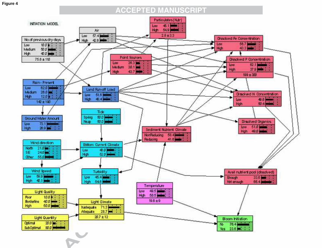
The static Science BN for initiation of Lyngbya is depicted in figure 4 with the 389

nodes representing the factors identified by the LSWG as important in the 390

initiation of a Lyngbya bloom. 391

392

(Place Figure 4 here) 393

394

ACCEPTED MANUSCRIPT 17

Sensitivity analysis of this BN revealed that the seven most influential factors 395

in the Science Network were (in decreasing order of influence): available 396

nutrient pool (dissolved), bottom current climate, sediment nutrients, dissolved 397

iron (Fe), dissolved phosphorous (P), light and temperature. Furthermore 398

scenario modelling consistently identified available nutrient pool as the factor 399

which most heavily influences the probability of initiation of a bloom. Point and 400

diffuse sources deliver nutrients to the bay and this nutrient delivery is 401

affected by management actions at the sources. 402

403

The Science BN was also interrogated using management and climatic 404

scenarios and analysing the effect on the probability of bloom initiation to 405

changes in the various factors. The predicted changes in the probability of a 406

Lyngbya bloom initiation as a result of each of the seven most influential 407

factors in isolation, is shown in Table 2. In a ‘typical’ year, as defined by the 408

LMWG, the probability of a bloom initiation was reported as 28%; this 409

increased significantly during a severe summer storm event to 42%, when 410

light climate was optimal and rain-present was high. Bloom initiation was a 411

predicted as a certainty (100%) when the available nutrient pool (dissolved) 412

was enough, temperature was high and light climate was optimal. However, 413

when only the available nutrient pool (dissolved) was set to ‘not enough’, the 414

probability of a bloom initiation dropped to 3%, but jumped to 80% when it 415

was changed to ‘enough’. Although bottom current climate was a key 416

influential factor, changing only this factor caused the probability of bloom 417

initiation to drop to 15% when the bottom current climate was ‘high’ and to 418

increase to 43% when it was ‘low’. This is a variation of 28% in the probability 419

ACCEPTED MANUSCRIPT 18

of a bloom initiation and although large, is clearly overshadowed by the 77% 420

variation caused by changes in nutrient availability. Changing iron availability 421

alone increased the probability of a bloom initiation from 21% to 37%. 422

Changing organics availability alone increased the probability of a bloom 423

initiation from 25% to 31%. 424

425

(Place Table 2 here) 426

427

Next the Science OOBN sub-network (figure 5) was created from the static 428

Lyngbya Science BN as outlined in Section 2.2, retaining all the key factors 429

(with the exception of the No of prev dry days) and their CPTs from the static 430

BN. As is characteristic of Object Oriented networks, the Science OOBN sub-431

network includes instances of other sub-networks, shown in figure 5 as 432

rectangles with rounded edges, such as the Wind subnet and the Turbidity 433

subnet. Input nodes were added to the Science OOBN sub-network as 434

placeholders for the real nodes, Temperature, Rain- present, Land Run-off 435

Load and Ground Water Amount. The sub-networks were based on the 436

groups created in the static Science BN to yield standalone networks capable 437

of linking to other networks via the interface nodes (input and output nodes), 438

or being instantiated in other networks. Importantly, providing the interface 439

remains intact, these OOBN sub-networks can be further expanded without 440

affecting the structure of any other networks linking to it. As a consequence 441

we have a powerful concept of parallel development by independent expert 442

teams while retaining the overall cohesive model. 443

444

ACCEPTED MANUSCRIPT 19

(Place Figure 5 here) 445

446

In collaboration with the LSWG and based on the findings of (Hamilton et al., 447

2007a) as described in Section 2.3, the static Lyngbya Science network was 448

adapted in the following manner to incorporate monthly rainfall and 449

temperature data and the lag effect of rainfall on the amount of groundwater 450

and land run-off. First, the lag effect of rainfall on groundwater amount and 451

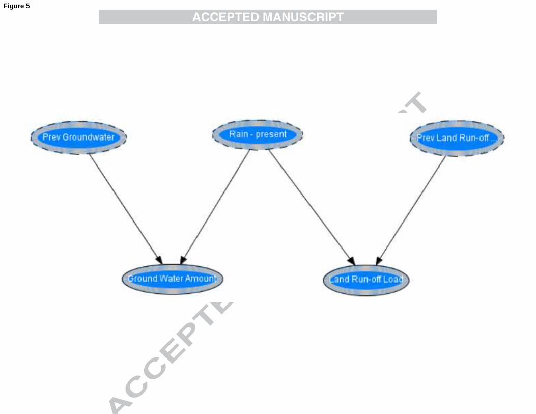
land run-off was replicated by creating a Rainwater OOBN sub-network as 452

shown in figure 6. In this OOBN, the Prev Groundwater and the Prev Land 453

Run-off are input nodes (double edged eclipse with a broken outer line), which 454

enable connectivity to the previous time slice’s Ground Water Amount and 455

Land Run-off nodes, respectively. The Rain – present input node enables the 456

instances of the Rainwater OOBN to be bound to the rainfall relating to that 457

instance, e.g. the November Rainwater OOBN instance will have November’s 458

rainfall bound to the Rain – present input node. The Ground Water Amount 459

and Land Run-off Load output nodes (double edged eclipse with a solid outer 460

line) make them visible to other networks and therefore allow them to be 461

bound to input nodes in other networks. 462

463

(Place Figure 6 here) 464

465

Finally the DOOBN was created with five time slices (figure 7), one time slice 466

for each of the summer months (December to February), one for the end of 467

spring (November) and one for the start of autumn (March) . Every time slice 468

has an instance of the Rainwater and Science sub-networks as well as the 469

ACCEPTED MANUSCRIPT 20

temperature and rainfall nodes for that month. Data from the Bureau of 470

Meteorology was used to quantify the DOOBN, as well as the information 471

contained in the initial static BN. 472

473

(Place Figure 7 here) 474

475

As can be seen in figure 8, the rainfall information for a particular month is 476

bound to the Rain present input node in the Rainwater and Science model 477

sub-network instances for that month and the Groundwater Amount and Land 478

Run-off output nodes from one month bind to the Prev Groundwater and Prev 479

Land Run-off input nodes of the following month, respectively. 480

481

(Place Figure 8 here) 482

483

The point and diffuse nutrient sources contributing to the Management 484

Network for Lyngbya initiation included: aquaculture, composting, onsite 485

sewage, poultry, waste disposal, waste water treatment plant, agriculture, 486

artificial development, development and clearing, extractive industries, 487

forestry, grazing, natural vegetation and stormwater. The sources and 488

nutrients identified by the management committee are shown in Table 3. 489

490

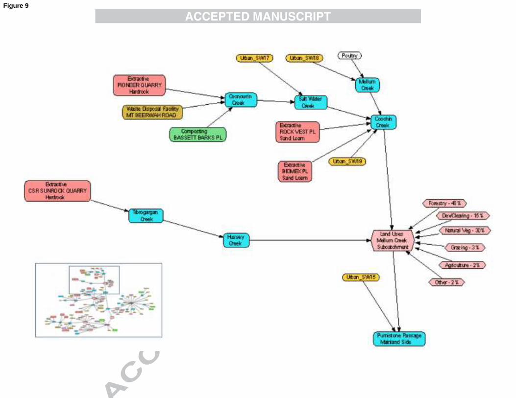
An extract of the Management Network, which identifies and locates point and 491

diffuse sources of nutrients for the Mellum Creek Sub-catchment, visually 492

represented in Netica®, is shown in figure 9. 493

494

ACCEPTED MANUSCRIPT 21

(Place Figure 9 here) 495

496

Scenario modelling predicted higher probabilities of Lyngbya bloom initiation 497

during the summer months and confirmed the temporal nature of Lyngbya 498

bloom initiation. Incorporating this behaviour resulted in the DOOBN for 499

Lyngbya bloom initiation (figure 7) being developed as outlined above with 500

one month lag effects included for groundwater amount and land run-off. 501

502

As shown in figure 10 below, the BN predicts a sharp increase in the 503

probability of initiation of a Lyngbya bloom from the end of spring (November) 504

to the first month of summer (December). The increased probability continued 505

during the next two summer months, with a slight fall in autumn (March). 506

Although these predicted probabilities for Lyngbya bloom initiation are low, the 507

increased trend in bloom initiation is clearly visible. When evidence of summer 508

rainfall was added to these time slices we observed a more dramatic 509

increase. For example, the probability of a bloom initiation was predicted as 510

52% when evidence of a summer rainfall event was entered into the 511

December time slice. This compares to 42% in the original static annual BN 512

model. 513

514

(Place Figure 10 here) 515

516

4 Discussion 517

This paper describes an Integrated Bayesian Network approach applied to the 518

initiation of Lyngbya blooms. The aim was to present the exposition of BN 519

ACCEPTED MANUSCRIPT 22

methodology to a complex ecological problem such as Lyngbya bloom 520

initiation and illustrate how it can be used to integrate models for different 521

aspects of the same issue. We have illustrated the process that could be 522

followed to integrate two static BNs and another type of model (such as the 523

E2 model of the Whole of Catchment) to achieve an integrated BN. The IBN 524

approach described here can also be used for investigating other features of 525

this organism, such as growth, biomass and decay, through appropriate 526

changes to the Science Network. These networks are currently being 527

developed. The Integrated Network approach is also conceptually suitable for 528

investigating other outcomes of interest that are impacted by nutrient outputs 529

and water movement in a catchment. 530

531

It is noted that it is beyond the scope of the present paper to provide an actual 532

test of the utility of BNs for predicting cyanobacterial blooms. The paper 533

therefore does not include a comparison of the predictions against classical 534

multivariate techniques; a test of the BNs own output reliability, that is, 535

whether the probabilistic estimate of the likelihood the BNs output is correct 536

for the target data set; a clear presentation of exactly what data are being 537

used; a sufficient amount of data to first build and refine the model on one 538

data set and then test it on a previously unseen set of data. However the 539

Science BN, which has been adopted by Healthy Waterways, will be validated 540

through future data collected as part of the next phase of the Lyngbya project. 541

542

More broadly, the general approach proposed in this paper is applicable to 543

environmental or other outcomes involving both scientific and management 544

ACCEPTED MANUSCRIPT 23

considerations. Information arising from expert knowledge, data and research 545

can be formally conceptualized and quantified through Science and 546

Management Networks, and combined into an Integrated Network. Such an 547

approach involves definition of the problem or outcome of interest, agreement 548

as to significant contributing factors and their definitions and pathways which 549

impact on this outcome, and identification and integration of information that 550

allow quantification of these factors and impacts. The benefits of such an 551

approach include a much greater specification of the issue at hand or 552

research focus, buy-in from diverse stakeholders, consolidation and 553

formalisation of information, an audit trail for decision-making and future 554

research, and quantitative outcomes in the form of probability statements 555

about the outcome of interest. 556

557

In the static Lyngbya BN (figure 4) similar factors were grouped together and 558

colour coded as a visual aid. The nature of the Science BN enabled a simple 559

conversion of the network to an OOBN (figure 6), with a sub-network for each 560

group of factors and interface nodes providing the communication links to 561

other OOBNs (figure 8). In the same way many complex BNs can be 562

simplified by abstracting the network to a higher level to include sub-networks 563

of logically grouped factors, which in turn can include other sub-networks, 564

thereby having several levels of abstraction. An important feature of the 565

OOBN sub-networks is that they can be developed simultaneously by the 566

various expert groups who are responsible for them. When the sub-networks 567

have been quantified, tested and ratified, they are integrated into the master 568

network containing instances of those sub-networks. 569

ACCEPTED MANUSCRIPT 24

570

The extension to a DOOBN not only improved prediction but also enhanced 571

interpretability of the network. The inclusion of time-specific dynamics for 572

temperature and water was more consistent with the conceptual framework of 573

Lyngbya behaviour held by both science and management stakeholders. 574

Moreover, it is more straightforward to include expert opinion and data of a 575

temporal nature in this expanded model. It is suggested that for other complex 576

ecological systems, the additional complexity of a DOOBN is more than 577

compensated for by the increased flexibility of representation of information 578

and acceptability of the outputs. 579

580

Finally, the creation of an IBN to combine multiple networks which describe 581

different aspects of an outcome of interest is an effective way of providing a 582

cohesive, quantifiable and auditable tool for better understanding and 583

coordination of multi-faceted environmental problems. 584

585

Acknowledgements 586

Financial assistance was provided by the Environmental Protection Agency 587

and Australian Government through the South East Queensland Healthy 588

Waterways Partnership, the ARC Centre for Dynamic Systems and Control, 589

and QUT Institute for Sustainable Resources. We fully acknowledge the 590

contributions of the Lyngbya Management Working Group and the Lyngbya 591

Science Working Group. For helpful comments on the manuscript we 592

acknowledge Kathleen Ahern, Barry Hart and an anonymous reviewer. 593

ACCEPTED MANUSCRIPT 25

594

References 595

Abal E G, Greenfield P F, Bunn S E and Tarte D M 2005 Healthy Waterways: 596

Healthy Catchments – An Integrated Research/Management Program 597

to Understand and Reduce Impacts of Sediments and Nutrients on 598

Waterways in Queensland, Australia, Frontiers of WWW Research and 599

Development - APWeb 2006: Springer Berlin / Heidelberg) pp 1126-600

1135 601

ABS 2004 3222.0 - Population Projections, Australia, 2004 to 2101. Australian 602

Bureau of Statistics) 603

Ahern K S, Ahern C R, Savige G M and Udy J W 2007 Mapping the 604

distribution, biomass and tissue nutrient levels of a marine benthic 605

cyanobacteria bloom (Lyngbya majuscula) Marine and Freshwater 606

Research 58 883-904 607

Ahern K S, Udy J W and Pointon S M 2006 Investigating the potential for 608

groundwater from different vegetation, soil and landuses to stimulate 609

blooms of the cyanobacterium, Lyngbya majuscula, in coastal waters 610

Marine and Freshwater Research 57 177-186 611

Ahmed B A, Matheny M E, Rice P L, Clarke J R and Ogunyemi O I 2009 A 612

comparison of methods for assessing penetrating trauma on 613

retrospective multi-center data Journal of Biomedical Informatics 42 614

308-316 615

Albert S, O’Neil J M, Udy J W, Ahern K S, O'Sullivan C M and Dennison W C 616

2005 Blooms of the cyanobacterium Lyngbya majuscula in coastal 617

ACCEPTED MANUSCRIPT 26

Queensland, Australia: disparate sites, common factors Marine 618

Pollution Bulletin 51 428-437 619

Angeli D, De Leenheer P and Sontag E D 2007 A Petri net approach to the 620

study of persistence in chemical reaction networks Mathematical 621

Biosciences 210 598-618 622

Arquitt S and Johnstone R 2004 A scoping and consensus building model of a 623

toxic blue-green algae bloom System Dynamics Review 20 179-198 624

Bednarski M, Cholewa W and Frid W 2004 Identification of sensitivities in 625

Bayesian networks Engineering Applications of Artificial Intelligence 17 626

327-335 627

Borsuk M E, Reichert P, Peter A, Schager E and Burkhardt-Holm P 2006 628

Assessing the decline of brown trout (Salmo trutta) in Swiss rivers 629

using a Bayesian probability network Ecological Modelling 192 224-244 630

Bromley J, Jackson N A, Clymer O J, Giacomello A M and Jensen F V 2005 631

The use of Hugin to develop Bayesian networks as an aid to integrated 632

water resource planning Environmental Modelling & Software 20 231-633

242 634

Coupe V M H, van der Gaag L C and Habbema J D F 2000 Sensitivity 635

analysis: an aid for belief-network quantification The Knowledge 636

Engineering Review 15 215-232 637

Dennison W C and Abal E G 1999 Moreton Bay Study: A Scientific Basis for 638

the Healthy Waterways: South East Queensland Regional Water 639

Quality Management Strategy) 640

Dennison W C, O’Neil J M, Duffy E J, Oliver P E and Shaw G R 1999 Blooms 641

of the cyanobacterium Lyngbya majuscula in coastal waters of 642

ACCEPTED MANUSCRIPT 27

Queensland, Australia Bulletin de l’Institut Oceanographique, Monaco 643

19 501-506 644

eWater CRC 2007 E2 Catchment Modelling Toolkit. 645

Fielding F, Alston C, Dwyer M, Hamilton G, Johnson S, McVinish R, Peterson 646

N and Mengersen K 2007 LYNGBYA Task 2.3: Development of an 647

Integrating Framework for the Lyngbya Research and Management 648

Program 2005-2007 Bayesian Belief Networks. (Brisbane, Australia: 649

Healthy Waterways Partnership) pp 1-39 650

Goss P J E and Peccoud J 1998 Quantitative Modeling of Stochastic Systems 651

in Molecular Biology by Using Stochastic Petri Nets Proceedings of the 652

National Academy of Sciences of the United States of America 95 653

6750-6755 654

Hamby D M 1994 A Review of Techniques for Parameter Sensitivity Analysis 655

of Environmental Models Environmental Monitoring and Assessment 656

32 135-154 657

Hamilton G, McVinish R and Mengersen K 2007a Bayesian model 658

identification and averaging for coastal algal bloom prediction. 659

Hamilton G, McVinish R and Mengersen K 2007b Bayesian model 660

identification and averaging for coastal algal bloom prediction 661

Ecological Applications in press 662

Hamilton G S, Fielding F, Chiffings A W, Hart B T, Johnstone R W and 663

Mengersen K 2007c Investigating the Use of a Bayesian Network to 664

Model the Risk of Lyngbya majuscula Bloom Initiation in Deception 665

Bay, Queensland Human and Ecological Risk Assessment 13 1271-666

1279 667

ACCEPTED MANUSCRIPT 28

Hepler A B and Weir B S 2008 Object-oriented Bayesian networks for 668

paternity cases with allelic dependencies Forensic Science 669

International: Genetics 2 166-175 670

Hugin 2007 Hugin. 671

Janssens D, Wets G, Brijs T, Vanhoof K, Arentze T and Timmermans H 2006 672

Integrating Bayesian networks and decision trees in a sequential rule-673

based transportation model European Journal of Operational Research 674

175 16-34 675

Jensen F V and Nielsen T D 2007 Bayesian Networks and Decision Graphs: 676

Springer Science + Business Media, LLC) 677

Kjaerulff U 1995 dHugin - a computational system for dynamic time-sliced 678

Bayesian networks International Journal of Forecasting 11 89-111 679

Koller D and Pfeffer A 1997 Object-Oriented Bayesian Networks. In: 680

Thirteenth Annual Conference on Uncertainty in Artificial Intelligence 681

(UAI-97), (Providence, Rhode Island pp 302-313 682

Laskey K B 1995 Sensitivity Analysis for Probability Assessments in Bayesian 683

Networks IEEE Transactions on Systems, Man and Cybernetics 25 684

901-909 685

Lauritzen S L, Dawid A P, Larsen B N and Leimer H G 1990 Independence 686

properties of directed Markov fields Networks 20 491-505 687

McCann R K, Marcot B G and Ellis R 2006 Bayesian belief networks: 688

applications in ecology and natural resource management1 Canadian 689

Journal of Forest Research 36 3053 690

Norsys 2007 Netica. 691

ACCEPTED MANUSCRIPT 29

Osborne N J, Shaw G R and Webb P M 2007 Health effects of recreational 692

exposure to Moreton Bay, Australia waters during a Lyngbya majuscula 693

bloom Environment International 33 309-314 694

Osborne N J T, Webb P M and Shaw G R 2001 The toxins of Lyngbya 695

majuscula and their human and ecological health effects Environment 696

International 27 381-392 697

Park M-H and Stenstrom M K 2008 Classifying environmentally significant 698

urban land uses with satellite imagery Journal of Environmental 699

Management 86 181-192 700

Paul V J, Thacker R W, Banks K and Stjepko G 2005 Benthic cyanobacterial 701

bloom impacts the reefs of South (Broward County, USA) Coral Reefs 702

24 693-697 703

Pearl J 1988 Probabilistic Reasoning in Intelligent Systems (San Francisco, 704

California: Morgan Kaufmann Publishers Inc) 705

Pollino C A, White A K and Hart B T 2007 Examination of conflicts and 706

improved strategies for the management of an endangered Eucalypt 707

species using Bayesian networks Ecological Modelling 201 37-59 708

Saddo A, Letcher R A, Jakemana A J and Newham L T H 2005 A Bayesian 709

decision network approach for assessing the ecological impacts of 710

salinity management Mathematics and Computers in Simulation 69 711

162–176 712

Stielow S and Ballantine D L 2003 Benthic cyanobacterial, Micro-coleus 713

lyngbyaceus, blooms in shallow, inshore Puerto Rican seagrass 714

habitats, Caribbean Sea Harmful Algae 2 127-133 715

ACCEPTED MANUSCRIPT 30

Taroni F, Aitken C, Garbolino P and Biedermann A 2006 Bayesian Networks 716

and Probabilistic Inference in Forensic Science: John Wiley & Sons, 717

Ltd) 718

Uusitalo L 2007 Advantages and challenges of Bayesian networks in 719

environmental modelling Ecological Modelling 203 312-318 720

Watkinson A J, O'Neil J M and Dennison W C 2005 Ecophysiology of the 721

marine cyanobacterium, Lyngbya majuscula (Oscillatoriaceae) in 722

Moreton Bay, Australia Harmful Algae 4 697-715 723

Weber P and Jouffe L 2006 Complex system reliability modelling with 724

Dynamic Object Oriented Bayesian Networks (DOOBN) Reliability 725

Engineering & System Safety 91 149-162 726

Wilson A G, Graves T L, Hamada M S and Reese C S 2006 Advances in Data 727

Combination, Analysis and Collection for System Reliability 728

Assessment Statistical Science 21 514–531 729

730

731

ACCEPTED MANUSCRIPT 31

732 Legends 733

Figure 1: UML use case diagram of the conceptual processes in the Lyngbya 734

bloom initiation Integrated Network 735

Figure 2: UML use case diagram of the processes for the Lyngbya bloom 736

initiation DOOBN 737

Figure 3: UML activity diagram detailing the processes for the Lyngbya bloom 738

initiation IBN 739

Figure 4: Science Network for Lyngbya initiation (Netica®) 740

Figure 5: Rainwater OOBN sub-network showing two output nodes, 741

Groundwater Amount and Land Run-off Load, which are then connected to 742

the input nodes Prev Groundwater and Prev Land Run-off in the next time 743

slice 744

Figure 6: Science OOBN sub-network 745

Figure 7: Five time slices forming the DOOBN for Lyngbya bloom initiation 746

Figure 8: Expanded sub-network instances in Hugin®, showing the interface 747

nodes for each instance. The input and output nodes are represented here as 748

ellipses with broken and solid lines, respectively. Also evident are the directed 749

links between the sub-network instances of the same and the next time slice, 750

so that information from one time slice can flow into the next time slice. 751

Figure 9: Extract of the Management Network for Mellum Creek Sub-752

catchment, a visual representation of the sub-catchment, showing point and 753

diffuse sources of nutrients. The inset shows the complete Management 754

Network 755

Figure 10: Probability of Lyngbya bloom initiation 756

ACCEPTED MANUSCRIPT 32

757 Table 1: Conditional probability table for Bottom Current Climate node with 758

states Low and High and parent nodes Wind Direction (states North, SE and 759

Other), Wind Speed (states Low and High) and Tide (states Spring and 760

Neap). These nodes, their states, probabilities and relationships are visible in 761

the Bayesian network in figure 4 762

763 Wind

Direction Wind Speed Tide Low High

North Low Spring 0.33 0.67 North Low Neap 0.61 0.39 North High Spring 0.43 0.57 North High Neap 0.54 0.46

SE Low Spring 0.42 0.58 SE Low Neap 0.58 0.42 SE High Spring 0.37 0.63 SE High Neap 0.59 0.41

Other Low Spring 0.39 0.61 Other Low Neap 0.59 0.41 Other High Spring 0.43 0.57 Other High Neap 0.50 0.50

764

ACCEPTED MANUSCRIPT 33

765 Table 2: Changes to the probability of Lyngbya bloom initiation for key 766

factors. All possible states for each of the nodes were assessed individually to 767

ascertain the delta effect it had on the probability of a Lyngbya bloom 768

initiation. 769

770

Factor Change in P(Bloom) (%)

Available Nutrient Pool 77 Bottom Current Climate 28 Sediment Nutrient Climate 17 Dissolved Fe 16 Dissolved P 15 Light Climate 14 Temperature 14

771

ACCEPTED MANUSCRIPT 34

772 Table 3: Point and diffuse sources contributing nutrients to Deception Bay 773

774 Source Point(P) or

Diffuse (D) Nitrogen Phosphorous Iron Organics

Aquaculture P X X Composting P X X Onsite Sewage P X X Poultry P X X X Waste Disposal P X X X Waste Water Treatment Plant P X X Agriculture D X X X X Artificial Development D X X Developing & Clearing D X X X X Extractive D X X Forestry D X X X X Grazing D X X Natural Vegetation D X X X Stormwater D X X 775 776

ACCEPTED MANUSCRIPT Figure 1

ACCEPTED MANUSCRIPT Figure 4

ACCEPTED MANUSCRIPT Figure 5

ACCEPTED MANUSCRIPT Figure 5

ACCEPTED MANUSCRIPT Figure 5

ACCEPTED MANUSCRIPT Figure 6

ACCEPTED MANUSCRIPT Figure 7

ACCEPTED MANUSCRIPT Figure 8

ACCEPTED MANUSCRIPT Figure 9

ACCEPTED MANUSCRIPT Figure 9

ACCEPTED MANUSCRIPT Figure 10

ACCEPTED MANUSCRIPT Figure 2

ACCEPTED MANUSCRIPT Figure 3