an integral equation approach for operators arising...
TRANSCRIPT

An Integral Equation Approach for Operators Arising From theIncompressible Navier-Stokes Equations
A Final Project for APMA930
Bryan Quaife
April 9, 2007
1 Introduction
The incompressible Navier-Stokes equations can be solved in various forms.In two dimensions, we have the luxury of being able to reduce the threeequations in the usual form to a single equation for a stream function. Theresult is that instead of two second order equations and the incompressibilityconstraint, we now have one fourth order partial differential equation (pde).
This fourth order pde can be discretized in time which leads to a fourthorder linear elliptic problem. Although standard methods for solving thistype of equation were introduced in APMA930, I will be discussing some ofthe theory necessary to solve parts of the problem as an integral equation.
In this report, I will first setup the stream function and discuss integralequations in sections two and three. Then, the scheme that I will be using isdescribed in the third section along with a brief discussion of the stability. Adiscussion of the numerical experiments as well as results from the numericalexperiments is found in the fifth section. Finally, some discussion of futurework and a conclusion of the results are in the last two sections.
2 The Stream Function
The stream function is simply a way to pose the Navier-Stokes equations. Itreduces the system of non-linear pdes to a single non-linear pde. It is thispde that I will be solving numerically.
2.1 The Equations
The incompressible Navier-Stokes equations in two dimensions form a systemof three coupled pdes. The notation that I will be using is
ut + uux + vuy = −px +1
Re∆u (1)
vt + uvx + vvy = −py +1
Re∆v (2)
ux + vy = 0. (3)
In the above equations, (1) and (2) is the conservation of momentum con-dition and (3) is the incompressibility condition. u and v are the x and ycomponents respectively of the velocity field, p is the pressure and Re is theReynolds number. The unknowns in the equations are u, v and p.
1

In two dimensions, we can reformulate the equations as follows. Considera function ψ : R2 → R, which will be called a stream function, which satisfies
ψy = u and ψx = −v.
Its mixed partials will commute and thus
ux + vy = ψyx − ψxy = 0.
That is, the incompressibility constraint (3) is automatically satisfied andthus can be disregarded from now on. Taking the curl of (1) and (2), weobtain the single fourth order equation
∂∆ψ
∂t− ∂ψ
∂y
∂∆ψ
∂x+∂ψ
∂x
∂∆ψ
∂y=
1
Re∆2ψ
where ∆2 is the usual biharmonic operator. There are three important ob-servations worth mentioning at this point. First, one should note that thepressure is now gone. After solving for ψ, one could solve for the pressuregradient by simply forming the sum
Op =1
Re∆u− ut − u · Ou
whereu := (u, v).
Secondly, another physical variable of interest is easily obtained. The vortic-ity, which is the curl of the velocity field is defined by w := vx−uy. In termsof the stream function,
w = vx − uy = −ψxx − ψyy = −∆ψ.
Finally, the streamlines of solutions to the Navier-Stokes are easy to obtainusing the stream function. Consider any level set (or contour line) of ψ.
2
Then,
C = ψ(x, y)
⇒0 =d
dxψ(x, y)
⇒0 = ψx + ψydy
dx
⇒dy
dx= −ψy
ψx
⇒dy
dx=v(x, y)
u(x, y)
which is exactly what characterizes streamlines.My interests are mostly concerned with numerically solving the fourth
order pde∂
∂t∆ψ − 1
Re∆2ψ =
∂ψ
∂y
∂∆ψ
∂x− ∂ψ
∂x
∂∆ψ
∂y
using integral equations. For the sake of simplifying the notation, I will usea Jacobian to represent the right hand side. That is, the fourth order pde is
∂
∂t∆ψ − 1
Re∆2ψ = J [∆ψ, ψ]. (4)
At this point, one can discretize the time derivative using some sort of finitedifference scheme and create a scheme having explicit and implicit parts. Aswe will see, this always leads to a pde of the form
(∆− α∆2)u = f
for some positive number α and some forcing term f . This operator can alsobe formulated as
∆− α∆2 = ∆(1− α∆).
Thus, we will dedicate the next section to formulating and solving integralequations for the three operators ∆− α∆2, 1− α∆ and ∆.
3

2.2 Boundary Conditions
Boundary conditions are necessary to impose on (4) in order to have a well-posed problem. I am only going to be considering boundary conditions de-fined on the boundary of the domain of the form
u · n = g1
u · s = g2.
Above, n is the unit outward normal and s is the unit tangent vector. Interms of the stream function, this gives the boundary conditions
(ψy,−ψx) · n = g1
(ψy,−ψx) · s = g2.
As n and s are always linearly independent, we can pose these two conditionsas one condition in terms of the gradient of ψ. Then we have the compactway of writing the boundary condition as
Oψ = G
for some vector valued function G. This function G is uniquely determinedby g1 and g2. So, the full fourth order equation with boundary conditionsof interest is
∂
∂t∆ψ − 1
Re∆2ψ = J [∆ψ, ψ]
Oψ = G.
One thing worth noting is that solutions to this problem are not unique.More particularly, if ψ is a solution to the pde with the correct boundarydata, then so is ψ + C for any constant C. However, this does not pose aproblem as the velocity field u is formed by taking derivatives of ψ.
3 Integral Equations
3.1 Formulation
Many homogeneous elliptic pdes can be solved using what are known asintegral equation methods. Consider a general second order homogeneouselliptic pde on a domain Ω ⊂ R2 of the form
Lu = 0 in Ω.
4
Give u either Dirichlet boundary data
u = f on ∂Ω
or Neumann boundary data
∂u
∂n= f on ∂Ω.
The goal is to write u as a convolution of some density function with somekernel. That is, find functions µ(x) and K(x) such that
u(x) =
∫∂Ω
K(x− y)µ(y)ds(y)
=: TK(µ)(x)
where ds is an arclength component. Above I am thinking of TK as theoperator that convolutes its argument against K.
The kernel is found by solving the equation
LK(x) = δ(x) in R2
where δ(x) is the usual delta distribution centered at the origin. There aregeneral methods for solving an equation of this kind and the kernels will begiven for all the operators of interest.
The more difficult task is finding the density function µ. This is wherethe integral equation comes into play. What is done is some kind of limitingprocess as points go through the boundary. For the operators we will beconsidering, this leads to an equation of the form
f(x) = λµ(x) +
∫∂Ω
K(x− y)µ(y)ds(y)
= λµ(x) + TK(µ)(x). (5)
Equation (5) is known as an integral equation for the function µ. f(x) isthe boundary data, regardless of if it is Dirichlet or Neumann and λ is somereal number. λ depends on the operator K, whether we have Dirichlet orNeumann boundary data and if we are solving an interior or exterior problem.All the coefficients λ, assuming an interior problem, will be given for each ofthe operators of interest.
5

Before we attempt to solve the integral equations, a word regarding theexistence of solutions is in order. We can rely on the Fredholm Alternativefor compact operators to discuss the existence of solutions. The operatorTK is a compact operator on L2(∂Ω) for all the elliptic problems we will beconsidering. Thus, the Fredholm Alternative does apply and it guarantees asolution to the integral equation (5) if the homogeneous problem
0 = λµ(x) +
∫∂Ω
K(x− y)µ(y)ds(y)
only has the trivial solution µ = 0. Depending on the domain and the kernelK, this may or may not be the case, but for the numerical experiments I willconsider in this report, the only homogeneous solution is the trivial solution.
Another result worth noticing is the computational cost of an integralequation formulation. Solving an integral equation numerically and per-forming point evaluation only requires studying functions on the boundaryof the domain. This substantially reduces the cost with comparison to typicalfinite difference schemes which require discretizing the entire domain. Thedownside to the integral equation is that the linear system that arises will bedense. This differs from the typical finite difference schemes which generallylead to some sort of banded sparse linear system.
3.2 The Operator ∆
The most common way of analytically solving Laplace’s equation with eitherNeumann or Dirichlet boundary data is via Green’s identities. First, onemust know the fundamental solution
Φ(x) := − 1
2πlog(x) (6)
which satisfies
∆Φ(x) = δ(x).
Then, applying Green’s third identity∫Ω
(u∆v − v∆u)dx =
∫∂Ω
(u∂v
∂n− v
∂u
∂n
)ds
6

with v(y) = Φ(x− y), we get
u(x) =
∫∂Ω
(u(y)
∂Φ(x− y)
∂ny
− Φ(x− y)∂u
∂ny
(y)
)ds(y).
At first glance, it appears that in order to solve Laplace’s equation, we requireNeumann boundary and Dirichlet boundary data. However, this is knownto be an overdetermined problem. At this point, one can replace the funda-mental solution (6) with the Green’s function for the domain, to eliminateone of the boundary integrals.
It is well-known [1] that one can also solve the interior Laplace equationin a simply connected domain Ω using an integral equation. For the Dirichletproblem where one has boundary data f , the solution is
u(x) =1
2π
∫∂Ω
∂
∂ny
log |x− y|µ(y)ds(y)
where
f(x) =1
2µ(x) +
1
2π
∫∂Ω
∂
∂ny
log |x− y|µ(y)ds(y).
For Neumann boundary data f , a solution is
u(x) =1
2π
∫∂Ω
log |x− y|µ(y)ds(y)
where
f(x) = −1
2µ(x) +
1
2π
∫∂Ω
∂
∂ny
log |x− y|µ(y)ds(y).
That is, the kernel is 12π
log |x| and the parameter λ from (5) is 12
for Dirichletboundary data and −1
2for Neumann boundary data.
One problem that one encounters when discretizing the boundary is thatwe will have to evaluate the kernel K(x − y) when x and y are arbitrarilyclose together. As the kernel is in terms of the logarithm function, this willpose a problem. However, it is easily shown using only l’hopital’s rule that
limy→x
∂
∂ny
log |x− y| = 1
2K(x)
7

where K(x) is the curvature of the boundary at the point x. The limit is as-sumed to be taken from the interior of the domain. That is, y is approachingx from inside Ω.
One other observation is that the integral equations for the Dirichlet andthe Neumann boundary data differ very slightly. It is only a minus sign thatdistinguishes the two equations.
3.3 The Operator 1− α∆
I have managed to derive very similar results concerning the operator 1−α∆where α is some positive real number. The first result is that
(1− α∆)1
2παK0
(|x− y|√
α
)= δ(x− y)
where Kn(x) is the nth modified Bessel function of the second kind. We willnow consider solving the problem
(1− α∆)u = 0 in Ω.
For Dirichlet boundary data f , the solution is
u(x) =1
2πα
∫∂Ω
∂
∂ny
K0
(|x− y|√
α
)µ(y)ds(y)
where
f(x) = − 1
2αµ(x) +
1
2πα
∫∂Ω
∂
∂ny
K0
(|x− y|√
α
)µ(y)ds(y).
For Neumann boundary data f , the solution is
u(x) =1
2πα
∫∂Ω
K0
(|x− y|√
α
)µ(y)ds(y)
where
f(x) =1
2αµ(x) +
1
2πα
∫∂Ω
∂
∂ny
K0
(|x− y|√
α
)µ(y)ds(y).
8
So, the parameter λ from (5) for this operator is −12α
for Dirichlet boundarydata and 1
2αfor Neumann boundary data. Notice again the very mild dif-
ference between integral equations for the Dirichlet boundary data and theNeumann boundary data.
As in the integral equation for Laplace’s equation, we will have difficultyevaluating the kernel as its argument goes to zero. I have proved a similarresult to that of the kernel of Laplace’s equation. Using l’hopital’s rule, onecan show that
limy→x
∂
∂ny
K0
(|x− y|√
α
)= −1
2K(x).
The limit again is understood to be taken from inside the domain Ω.
3.4 The Operator ∆− α∆2
Having the two previous integral equation formulations for the operators ∆and 1−α∆, an integral equation for ∆−α∆2 nearly comes for free. Considerthe problem
(∆− α∆2)u = 0 in Ω.
First, we need to find the kernel K(x) satisfying
(∆− α∆2)K(x) = δ(x).
Based on the kernels of the two previous operators, one can predict that
K(x) = C1 log |x|+ C2K0
(|x|√α
).
Then,
(∆− α∆2)K(x) = (∆− α∆2)
(C1 log |x|+ C2K0
(|x|√α
))= C1(1− α∆)∆ log |x|+ C2∆(1− α∆)K0
(|x|√α
)= −2πC1(1− α∆)δ(x) + 2παC2∆δ(x)
= δ(x)(−2πC1) + ∆δ(x)(2παC1 + 2παC2).
9
Then matching coefficients we have that
K(x) = − 1
2πlog |x|+ 1
2πK0
(|x|√α
).
A result concerning the evaluation of the kernel when its argument goes tozero is also easy to derive. We have that
limy→x
∂
∂ny
(− log |x− y|+K0
(|x− y|√
α
)= −K(x).
The difficulty with the scheme comes into play with the boundary data. Onecan easily find a solution with Dirichlet boundary data f by setting
u(x) =1
2π
∫∂Ω
∂
∂ny
(− log |x− y|+K0
(|x− y|√
α
))µ(y)ds(y)
where
f(x) = −µ(x) +1
2π
∫∂Ω
∂
∂ny
(− log |x− y|+K0
(|x− y|√
α
))µ(y)ds(y).
If one wants to satisfy Neumann boundary data f , a solution is
u(x) =1
2π
∫∂Ω
(− log(|x− y|+K0
(|x− y|√
α
))µ(y)ds(y)
where
f(x) = µ(x) +1
2π
∫∂Ω
∂
∂ny
(− log |x− y|+K0
(|x− y|√
α
))µ(y)ds(y).
However, as both these problems are under determined, it is not yet knownwhich solution the integral equation will return. That is, if we impose Dirich-let boundary data, the Neumann boundary data that the integral equationwill return is unknown and vice versa. For now, the most promising ideais to use two density functions. That is, if we are given Dirichlet boundarydata f and Neumann boundary data g, then look for a solution of the form
u(x) =1
2π
∫∂Ω
∂
∂ny
(− log |x− y|+K0
(|x− y|√
α
))µ1(y)ds(y)
+1
2π
∫∂Ω
(− log |x− y|+K0
(|x− y|√
α
))µ2(y)ds(y).
10

This would lead to a system of integral equations for µ1 and µ2 which I havenot yet been able to pose.
Assuming the geometry is extremely simple, there is an easy fix to getaround this fact that I am not yet able to implement all the boundary con-ditions of this fourth order equation. This will be discussed when I discussthe scheme.
3.5 Solving Integral Equations Numerically
We are now ready to discretize the integral equation. We cut up the boundaryof the domain ∂Ω into n equal pieces (whether this is done with respect toarclength or some other type of parametrization is irrelevant) and setup alinear system. Define the vector f and the vector µ by
f = (f(x1), f(x2), . . . , f(xn))
µ = (µ(x1), µ(x2), . . . , µ(xn))
where x1, x2, . . . , xn are the discrete points on ∂Ω. Then, the integral equation(5) is replaced by the linear system
f(xi) = λµ(xi) +n∑
j=1
K(xi − yj)µ(yj)∆syj
for all i = 1, . . . , n. These are n linear equations for the unknowns µ(x1), . . . , µ(xn).Call the matrix associated to this linear system K. That is
Kµ = f .
The nature of the integral equation causes the matrix K to be dense.However, preliminary results for simple domains show that even though thismatrix is dense it is extremely well-conditioned. As well, it has the phe-nomenon that increasing the number of points on the boundary does notincrease the condition number of the system. Thus, it is an ideal system forusing an iterative technique such as GMRES to solve the linear system.
The integral equation method can also be solved numerically in sucha manner that we get spectral convergence. This has been achieved forLaplace’s equation in [2].
11

4 The Scheme
From now on, the only domain we are going to be working in is the unit disccentered at the origin. The long term goal is to able to use integral equationsto solve for the stream function in arbitrary geometries.
Recall that we are trying to solve the pde in equation (4) with the gra-dient on the boundary specified to be G. For the sake of simplicity, I amgoing to use a first order scheme in time and treat the nonlinear terms in anobvious manner. A higher order finite difference could be used to increasethe accuracy in time without much more effort. To approximate (4), thescheme of interest is
∆ψN+1 −∆ψN
∆t− 1
Re∆2ψN+1 = J [∆ψN , ψN ].
Rearranging, we have
∆ψN+1 − ∆t
Re∆2ψN+1 = ∆ψN + ∆tJ [∆ψN , ψN ]. (7)
At this point, it is crucial to notice that this is simply the pde we werestudying in the previous section. That is, we are solving
(∆− α∆2)u = f
where
u = ψN+1
α =∆t
Ref = ∆ψN + ∆tJ [∆ψN , ψN ].
In order to solve this pde with the appropriate boundary conditions, I de-compose the solution as ψ = ψP + ψH where
(∆− α∆2)ψP = f in Ω
ψP = 0 on ∂Ω
and
(∆− α∆2)ψH = 0 in Ω
OψH = G− OψP on ∂Ω.
That is, ψP imposes the forcing term and ψH corrects for the boundarycondition.
12
4.1 The Particular Problem
I solve the particular problem with finite differences. To do this, I firstdecompose the fourth order equation into the two second order equations bydefining w := ∆ψP . Then I solve
(1− α∆w) = f
with zero Dirichlet boundary data. As we are working in the unit disc, I firstconsider the operator in polar coordinates as
1− α
(∂2
∂r2+
1
r
∂
∂r+
1
r2
∂2
∂θ2
).
Define the usual notation
wi,j := w(ri, θj)
where ri are the discrete values for the radius and θj are the discrete values forthe angle between the discrete point and the positive x axis, or the abscissa.I use the second order scheme
wi,j − α
(wi+1,j − 2wi,j + wi−1,j
∆r2+
1
i∆r
wi+1,j − wi−1,j
2∆r+
1
i2∆r2
wi,j+1 − 2wi,j + wi,j−1
∆θ2
)= fi,j
for all interior points except the origin. The Dirichlet boundary data is easilyimplemented in the scheme by replacing these values with zeros wheneverthey appear in the scheme.
The vector of unknowns that I am solving for is
w = (w0,0, w1,0, w1,1, . . . , w1,N−1, . . . , wM−1,0, wM−1,1, . . . , wM−1,N−1)
where
M∆r = 1 and N∆θ = 2π.
Notice that only one abscissa is used when r = 0 as w0,j corresponds to thesolution at the origin regardless of j.
At the origin, the 1∆r
term causes a problem as the scheme is forced todivide by zero. As we do not have boundary data at the origin, we can onlyuse the fact that we need the solution to be bounded. We do not yet have
13

an equation for the solution at the origin, so we still have one more linearequation we can put into the scheme. The code I am using approximates thesolution at the origin by using the average solution at the two previous radii.What is done is a line is fitted to the average values of the solution at the twoprevious radii and then the solution at the origin is extrapolated off of thisline. There is not a whole lot of justification to this method except that itseems to keep the scheme stable and returns a reasonable rate of convergence.Although the linear extrapolation is only based on a first order method, itshould not cause the solution well inside the domain to be less than secondorder.
Next, I solve the Poisson equation
∆ψP = w
with Dirichlet boundary data. This is almost a carbon copy of the previousparticular problem except that some of the coefficients in the matrix change.Where the coefficients are placed remains fixed. I use the same strategy forthe boundary data and the solution at the origin.
A plot indicating where there are non-zero entries (sparsity plot) is in-cluded. It corresponds to a system where there are only 5 radial and 8abscissa discretizations.
There are some key features to no-tice about the structure of this ma-trix. First, it is nearly in the typi-cal tridiagonal sparse matrix form.Even though I have simply usedthe backslash operator in matlab,one could use some kind of sparsematrix solver. Next, there are afew coefficients on the edges of thematrix. The entries on the left handside correspond to the fact that at
level ∆r, all the points use the origin as part of their solution. The entries onthe bottom correspond to the linear extrapolation that was used to obtaina solution at the origin. The last thing to notice is how the periodicity intheta is built in. This can be seen in the zoomed in version of the sparsityplot.
14

This zoomed in version of the spar-sity plot shows part of the sevenequations for the different abscissaat a single radius. The two entriesin the top right corner and the bot-tom left corner demonstrate the pe-riodicity in theta.
I have also included a plot show-ing the rate of convergence in theradial direction for the Poisson equa-tion. Here, the number of abscissadiscretized points is held fixed and the number of radial discretized points isallowed to vary. I am expecting second order convergence.
The forcing term in the partic-ular solution was taken to be f = 1so that the unique solution is
w(x, y) =x2 + y2 − 1
4.
All the errors were measured in the`1 norm. The slope of the line is ap-proximately equal to -2.1771 indi-cating a second order scheme withrespect to the radius.
As for the rate of convergence with respect to the abscissa, forming anactual plot indicating the rate of convergence is very difficult to do. However,there should be no trouble getting second order convergence with respect toθ as we did use a second order approximation for the only derivative withrespect to θ that arises in the equations. Thus, the overall rate of convergenceof the particular solution of (7) is second order.
4.2 The Homogeneous Problem
The homogeneous problem is where the integral equations will eventuallycome into play. Currently, the difficulty lies in assuring that all the boundaryconditions of the fourth order equation are satisfied. However, there is a wayaround it based on the geometry of the domain. The homogeneous problem
15

in polar coordinates is
(∆− α∆2)ψH(r, θ) = 0 in Ω (8)
OψH(1, θ) = (g1(θ), g2(θ)) on ∂Ω
where
(g1(θ), g2(θ)) = G(θ)− OψP (1, θ).
First, define the complex valued function g(θ) = g1(θ) + ıg2(θ). Next, thebounded radially symmetric solutions to the homogeneous problem are
AnIn
(r√α
)+Bnr
|n|
where In(r) is the modified Bessel function of the first kind. With the knowl-edge of the radially symmetric solutions, we can write the homogeneous so-lutions as
ψH(r, θ) =
(AnIn
(r√α
)+Bnr
|n|)eınθ.
Then, we simply match coefficients so that OψH(1, θ) agrees with
g(θ) =∑n∈Z
gneinθ.
Before the coefficients are given, one should note that the scheme is extremelyfast as I have implemented the fast Fourier transform. However, we can onlyuse finitely many Fourier coefficients in the sum, but this does not limit theaccuracy of the scheme if enough discrete points are taken on ∂Ω.
It is discussed in [3] that the coefficients An are given by
A0 =
√αg0
I1(1/√α)
An =
√αgn
In+1(1/√α)
n ≥ 1
An =A−n n ≤ −1,
16

and the coefficients Bn are given by
Bn =1
2n
An√αIn+1
(1√α
)− gn n ≤ −1
Bn =B−n n ≥ 1.
The one coefficient that we have not defined is B0. This can in fact be anynumber you want as it corresponds to adding a constant to the solution.Thus, my code simply sets it to be zero.
Two plots indicating the rate ofconvergence are include. The firstcorresponds to the error with re-spect to the radial direction andthe second corresponds to the er-ror with respect to the abscissa di-rection. As I am using a spectralcode, I expect the error to be ex-tremely small. Both plots indicatethat the scheme gives a solutionaccurate to no less than fifteen dec-
imal places in the `1 norm. That is, the error does seem to be spectral. Theboundary data that I took to study the order of convergence was
∂ψH
∂n= cos(θ) + sin(θ)
∂ψH
∂s= cos(θ)− sin(θ).
This is the boundary data of ψH(r, θ) = r cos(θ) + r sin(θ) which solves (8).
17
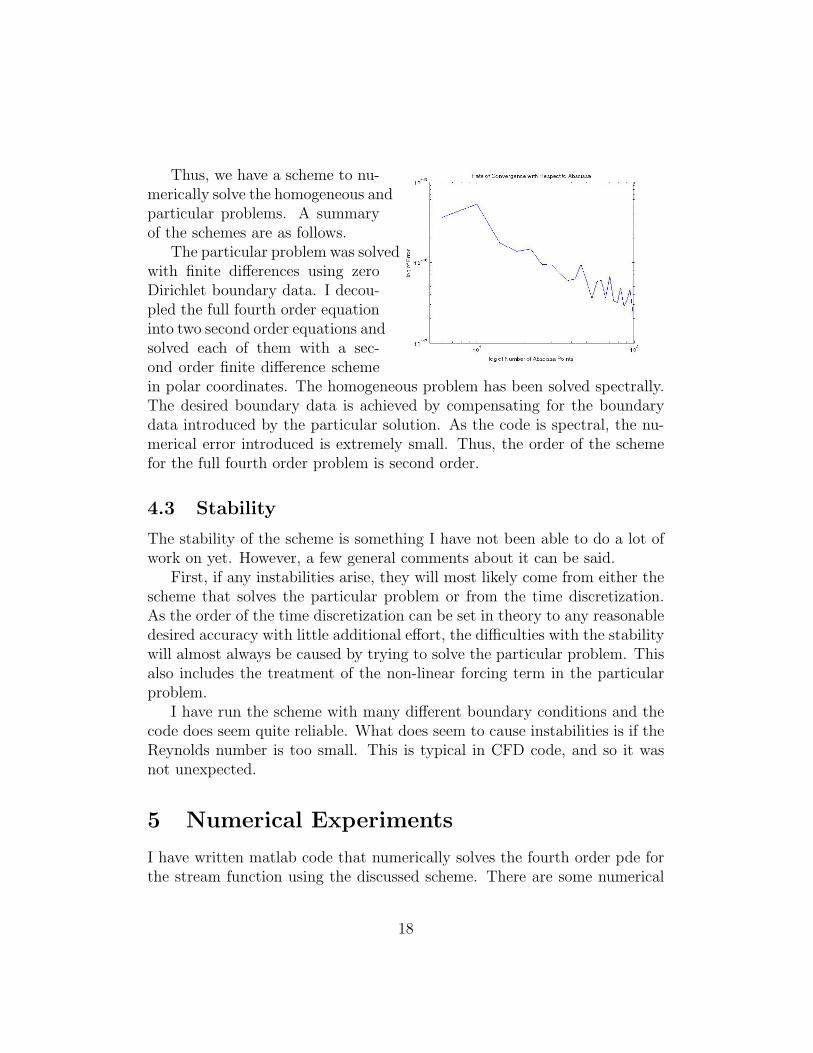
Thus, we have a scheme to nu-merically solve the homogeneous andparticular problems. A summaryof the schemes are as follows.
The particular problem was solvedwith finite differences using zeroDirichlet boundary data. I decou-pled the full fourth order equationinto two second order equations andsolved each of them with a sec-ond order finite difference schemein polar coordinates. The homogeneous problem has been solved spectrally.The desired boundary data is achieved by compensating for the boundarydata introduced by the particular solution. As the code is spectral, the nu-merical error introduced is extremely small. Thus, the order of the schemefor the full fourth order problem is second order.
4.3 Stability
The stability of the scheme is something I have not been able to do a lot ofwork on yet. However, a few general comments about it can be said.
First, if any instabilities arise, they will most likely come from either thescheme that solves the particular problem or from the time discretization.As the order of the time discretization can be set in theory to any reasonabledesired accuracy with little additional effort, the difficulties with the stabilitywill almost always be caused by trying to solve the particular problem. Thisalso includes the treatment of the non-linear forcing term in the particularproblem.
I have run the scheme with many different boundary conditions and thecode does seem quite reliable. What does seem to cause instabilities is if theReynolds number is too small. This is typical in CFD code, and so it wasnot unexpected.
5 Numerical Experiments
I have written matlab code that numerically solves the fourth order pde forthe stream function using the discussed scheme. There are some numerical
18

experiments in [3] that solve this problem in a similar manner. I ran my codewith some of the same boundary data that is in [3] as well as some boundarydata that I thought would give some interesting results.
Example For this example, I will solve for the stream function starting withan initial profile of zero and boundary conditions
∂u
∂n= 0
∂u
∂s= −1
2(1 + cos(θ)).
This corresponds to a fluid initially at rest and driven by a boundary rotatingin the clockwise direction with varying speed. The code was run until it wasnear steady state.
Figure 1: The Streamlines and Vorticity Contour Lines for Re = 16
The two different Reynolds numbers that I used were 16 and 100. InFigures 1 and 2, the left plots correspond to the streamlines and the rightplots correspond to the contour lines of the vorticity. The results seem to beconsistent with those found in [3].
Example This example is setup exactly the same as the previous exceptthat the boundary condition is
∂u
∂n= 0
∂u
∂s= − cos(θ) sin(θ).
19
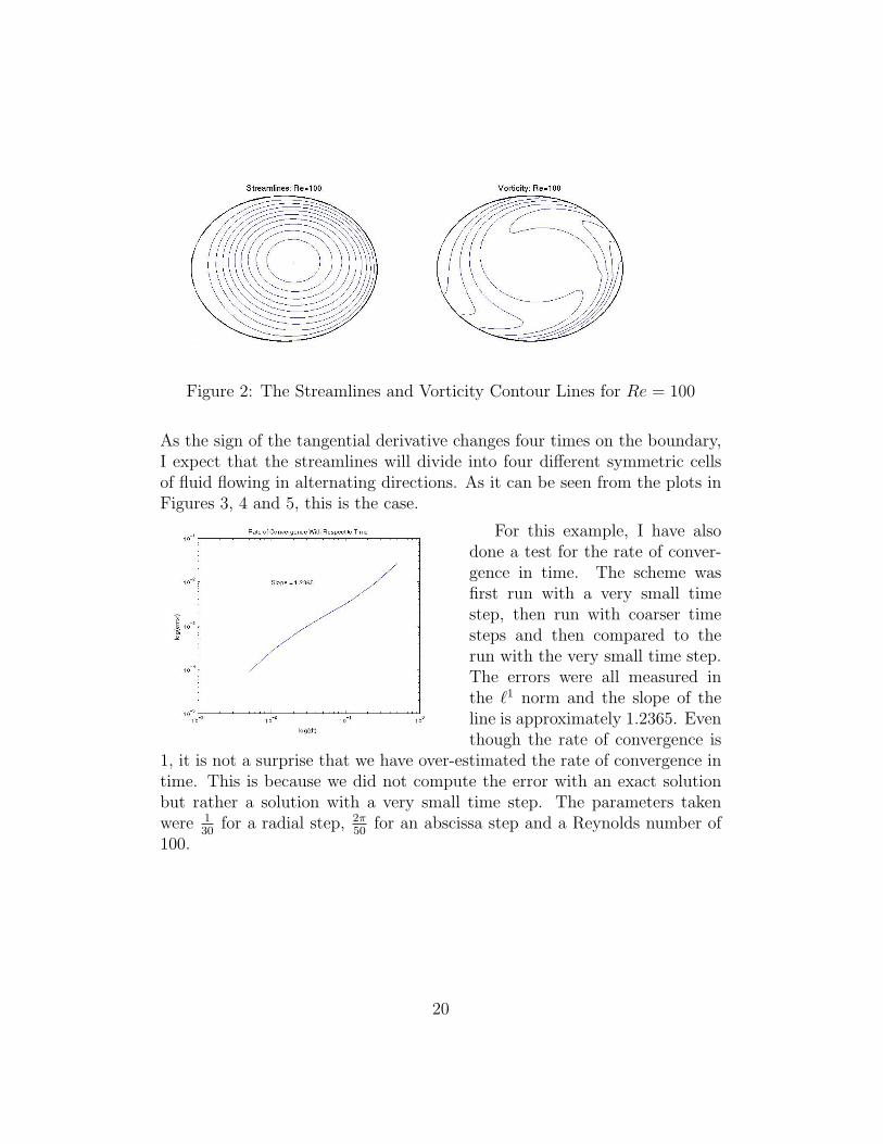
Figure 2: The Streamlines and Vorticity Contour Lines for Re = 100
As the sign of the tangential derivative changes four times on the boundary,I expect that the streamlines will divide into four different symmetric cellsof fluid flowing in alternating directions. As it can be seen from the plots inFigures 3, 4 and 5, this is the case.
For this example, I have alsodone a test for the rate of conver-gence in time. The scheme wasfirst run with a very small timestep, then run with coarser timesteps and then compared to therun with the very small time step.The errors were all measured inthe `1 norm and the slope of theline is approximately 1.2365. Eventhough the rate of convergence is
1, it is not a surprise that we have over-estimated the rate of convergence intime. This is because we did not compute the error with an exact solutionbut rather a solution with a very small time step. The parameters takenwere 1
30for a radial step, 2π
50for an abscissa step and a Reynolds number of
100.
20

Figure 3: The Streamlines and Vorticity Contour Lines for Re = 100
Figure 4: The Streamlines and Vorticity Contour Lines for Re = 300
Figure 5: The Streamlines and Vorticity Contour Lines for Re = 1000
Example For a final example, consider a flow with no penetration on theentire boundary but a discontinuous tangential derivative. I have used the
21

boundary data
∂u
∂n= 0
∂u
∂s= signum(sin(3πθ))
where
signum(x) :=x
|x|x 6= 0
signum(0) := 0.
The tangential derivative changes discontinuously from -1 to 1 numeroustimes on the boundary of the domain. The purpose of this example is to firstshow some interesting looking streamlines and vorticity contour lines andsecondly to demonstrate that the code can iterate on discontinuous boundarydata without going unstable.
Figure 6: The Streamlines and Vorticity Contour Lines for Re = 20
Figure 7: The Streamlines and Vorticity Contour Lines for Re = 100
22
Reynolds numbers of 20 and 100 were taken. The simulation for Reynoldsnumber 20 reached a steady state after about time 12 and is plotted in Figure(6). The simulation for Reynolds number 100 was run until time 50 and isplotted in Figure (7). Both codes had a time step of 0.1.
6 Future Work
There is still a lot of work to be done with this method. A few of them arelisted below.
• Use a true integral equation method to solve all the necessary homo-geneous problems.
• Use an iterative technique to solve all the linear systems.
• Treat the nonlinear term in a more sophisticated manner to increasethe accuracy.
• Generalize the code to arbitrary geometries including exterior problemsand multiply connected domains.
• Avoid polar coordinates as it does not have a uniform resolution.
• Increase the order of accuracy of the particular problem so that itcompares to the order of accuracy of the integral equation method.
• Implement the Fast Multipole Method (FMM) whenever possible toincrease the cost of the entire algorithm to order N where N is thenumber of grid points on ∂Ω.
• Come up with interesting boundary data to test.
7 Conclusions
In this report I have discussed some of the theory necessary to solve a fourthorder equation for the stream function using integral equations. An integralequation method is potentially very fast and very accurate. As I have not yetfully derived all the theory to solve the integral equations arising from the
23

stream function, an alternative method was used to look at some preliminarynumerical results.
The original fourth order pde for the stream function was discretized intime leading to a fourth order linear pde at each time step. These equationswere split into a homogeneous and particular problem. The particular prob-lem was solved using a finite difference scheme. The homogeneous problemcorrected for the boundary data introduced by the particular problem andwas solved using a spectral code.
The methods introduced in this report have a lot of promise in solvingthe stream function in arbitrary geometries not only accurately, but rapidly.Thus, there is a lot of promising results that can be found in this line ofresearch.
24
References
[1] Gerald B. Folland. Introduction to Partial Differential Equations. Prince-ton University Press, second edition, 1996.
[2] A Greenbaum and L. Greengard. Laplace’s equation and the dirichlet-neumann map in multiply connnected domains. Journal of ComputationalPhysics, 105:267–278, 1993.
[3] Leslie Greengard and Mary-Catherine Kropinski. An integral equationapproach to the incompressible navier-stokes equations in two dimensions.SIAM Journal of Scientific Computing, 1998.
25