an incidence loss model for wave rotors with axially ... · an incidence loss model for wave rotors...

NASA/TM--1998-207923 AIAA-98-3251

An Incidence Loss Model for Wave Rotors

With Axially Aligned Passages

Daniel E. Paxson

Lewis Research Center, Cleveland, Ohio

Prepared for the

34th Joint Propulsion Conference

cosponsored by AIAA, ASME, SAE, and ASEE

Cleveland, Ohio, July 12-15, 1998

National Aeronautics and

Space Administration

Lewis Research Center

June 1998

https://ntrs.nasa.gov/search.jsp?R=19980210003 2018-07-17T10:32:49+00:00Z

NASA Center for Aerospace Information7121 Standard Drive

Hanover, MD 21076Price Code: A03

Available from

National Technical Information Service

5287 Port Royal Road

Springfield, VA 22100Price Code: A03

AIAA-98-3251

AN INCDENCE LOSS MODEL FOR WAVE ROTORS

WITH AXIALLY ALIGNED PASSAGES

Daniel E. Paxson t

NASA Lewis Research Center

Cleveland, Ohio, USA

Abstract

A simple mathematical model is described to accountfor the losses incurred when the flow in the duct (port)

of a wave rotor is not aligned with the passages. The

model, specifically for wave rotors with axially aligned

passages, describes a loss mechanism which is sensitiveto incident flow angle and Mach number.

Implementation of the model in a one-dimensional CFD

based wave rotor simulation is presented. Comparisons

with limited experimental results are consistent with the

model. Sensitivity studies are presented which highlight

the significance of the incidence loss relative to otherloss mechanisms in the wave rotor.

Introduction

Inlet flowfields of nearly any wave rotor typically

contain significant velocity non-uniformities. This is

true for both on and off-design operation. The non-uniformities arise from, among other causes, mis-timed

waves in the passages, and reflected expansion waves offinite width. From the reference frame of the rotor

passages, the non-uniformities result in inflow incidence

angles which can be severe, and can in turn result inlarge relative total pressure losses. Despite the largelosses in the relative frame however, incidence can

result in work being done on (or by) the entering flow,

which can affect the overall performance of the

machine. Thus, accurate predictions of wave rotor

performance requires adequate accounting of theseeffects. In the case of two and three-dimensional

unsteady CFD calculations they are computed directly)

For unsteady one-dimensional, and steady . two-dimensional calculations however, they must be

modeled. 2_ Unfortunately, little has been found in theliterature, either theoretical or experimental, to shed

light on an appropriate modeling approach.

This paper presents a model which has been

implemented in a one-dimensional CFD based waverotor simulation 4. It applies specifically to wave rotor

configurations in which the passages are aligned with

t Member AIAA

Copyright © 1998 by the American Institute of Aeronautics and Astronautics,

Inc. No copyright is asserted in the United States under Title 17, U.S. Code.

"nae U.S. Government has a royalty-free license to exercise all rights under the

copyright claimed herein for Governmental Purposes. All other rights are

reserved by the copyright owner.

NASA/TM--1998-207923

_U

Figure 1 Incidence Flow Schematic

the axis of rotation (e.g. pressure exchange machines);

however, it could be modified to include more general

configurations. It produces realistic loss estimates over

a wide range of incidence angles, at low to moderateincident Mach numbers. The model and its

implementation are described. Comparisons are thenmade between simulated data and those from the NASA

Lewis 3-port wave rotor experiment 5. These include

both limited dynamic pressure traces within a wave

rotor passage in a high incidence region of a wave rotorflowfield, and averaged port performance data. The

relative significance of incidence losses are then

compared to other (modeled) loss mechanisms by wayof simulated performance maps with various models'turned on' or 'off'. The results will show that

incidence losses can be at least as significant as other

major losses such as those due to finite passage opening

time, leakage, or friction.

Model Description

A schematic diagram of the envisaged flowfield, alongwith relevant nomenclature is shown in Fig. 1. It is

shown again in Fig. 2 from the reference frame of a

passage. Flow entering the passage at incidence forms a

separated region, or vena contracta. The flow thenreattaches downstream having lost relative total

pressure (momentum) primarily due to the shear stressat the boundary between recirculating, separated flow

American Institute of Aeronautics and Astronautics

_ sepam_egion

G

Figure 2 Incidence Flow Schematic From PassagePerspective

and that which passes directly through.

To estimate the total pressure loss, several

simplifications are made. First, the flow to the left of

plane t in Fig. 2 and outside the separated region is

assumed isentropic. Second, the flow in plane t, butoutside the separated region, as well as the flow in

region 2 is assumed parallel to the passage. Third, the

static pressure in plane t is constant, and there is no netvelocity in the separated region. These assumptions

imply that the losses are kinematically equivalent to

those of a backward facing step of height h shown in

Fig. 2. The gas is also assumed calorically perfect.

The maximum height of the separated region h is

considered a function the incidence angle i. The

particular choice of this functionality used in the presentmodel is based upon a low speed (e.g. incompressible)

incidence loss model which may be written as

AP°2 = sin2(i)low 2 (I)

where w is the relative velocity in Fig. 2. This relation,suggested by Roelke 6 arises from the assumption that all

of the kinetic energy in region 1 which is normal to thepassage of region 2 is lost at constant mean static

pressure.

Using Eqn. 1, the assumptions described above, and the

incompressible equations of mass and momentum from

plane t to region 2, the following relationship for h isobtained

h Isin(i)l

b Isin(i)l+ cos(i)(2)

0.6

0.5

•.; 0.4

"B

0.3

0.2

0.1

/

I

!

I

I

I

I

I

I

I ./°

I /"

i I //

I ,°°°°

/ o.O°

l oO°°

I .°°°

/ °o°°

/ .°""

j °oO-°"

j .°,°

0 10 20 30

Dam of Emmm

Sharp no_l blades

Model

l_cid_mt Math Nu_.2

Prater Model

Tau:id_atMada Number--0.5

0 I ,

40 50 60

Incidence Angle, i (deg.)

Figure 3 Experimental vs. Modeled Loss

Coefficients for a Sharp Nosed Turbine Cascade.

where b is the passage height shown in Fig. 2. Using

the nomenclature of Fig. 1, this may be rewritten as

h V sin(_l)- U

= V sin(I]) - U + V cos(I])(3)

Where V is the absolute velocity upstream and U is the

rotor speed. Of course, since Eqn. 3 is derived from

Eqn. 1 it will yield the same total pressure loss.Equation 1 has simply been reinterpreted; however, it is

strictly incompressible. Compressibility effects may be

included by assuming that Eqn. 3 remains valid;however, the mixing calculation from the throat region,

t to region 2 now becomes a compressible mass

momentum and energy balance, namely

h

ptwt (1 - _-)= P2W2 (4)

hPt +PtWt2(1-_)=P2 +p2w2 (5)

ptwt(1-h)(y-1)H =(,yP2w2+_-_p2w2 3) (6)

a 2 w 2where H t =- +--, and a is the local speed of

y-1 2

sound. The shear stress at the walls is assumed

negligible and the flow is considered isentropic in

region 1. Thus, if absolute stagnation conditions, wheel

speed, duct angle 9, and static pressure Pl are known in

region 1 of Fig. 2, then Eqns. 3-6 may be used to find

conditions in region 2.

NASA/TM--1998-207923 2American Institute of Aeronautics and Astronautics

1.15

1.10Q

t_1.05

_ 1.00

0.95

0.90

present isentropic Eqn. 1model

0.00 0.05 0.10 0.15 0.20 0.25 0.30 0.35

Normalized Inlet Mass Flow rate

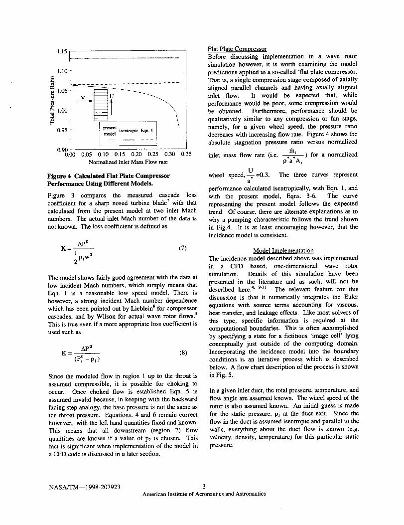
Figure 4 Calculated Flat Plate Compressor

Performance Using Different Models.

Figure 3 compares the measured cascade loss

coefficient for a sharp nosed turbine blade 7 with that

calculated from the present model at two inlet Mach

numbers. The actual inlet Mach number of the data is

not known. The loss coefficient is defined as

Ap °K=--

lpl w2

(7)

The model shows fairly good agreement with the data at

low incident Mach numbers, which simply means that

Eqn. 1 is a reasonable low speed model. There is

however, a strong incident Mach number dependence

which has been pointed out by Lieblein s for compressor

cascades, and by Wilson for actual wave rotor flows. 5

This is true even if a more appropriate loss coefficient is

used such as

_kp °

K - (8)

(pO _ Pl)

Since the modeled flow in region 1 up to the throat is

assumed compressible, it is possible for choking to

occur. Once choked flow is established Eqn. 5 is

assumed invalid because, in keeping with the backward

facing step analogy, the base pressure is not the same as

the throat pressure. Equations. 4 and 6 remain correct

however, with the left hand quantities fixed and known.

This means that all downstream (region 2) flow

quantities are known if a value of P2 is chosen. This

fact is significant when implementation of the model in

a CFD code is discussed in a later section.

Flat Plate Compressor

Before discussing implementation in a wave rotor

simulation however, it is worth examining the model

predictions applied to a so-called 'fiat plate compressor.

That is, a single compression stage composed of axially

aligned parallel channels and having axially aligned

inlet flow. It would be expected that, while

performance would be poor, some compression would

be obtained. Furthermore, performance should be

qualitatively similar to any compression or fan stage,

namely, for a given wheel speed, the pressure ratio

decreases with increasing flow rate. Figure 4 shows the

absolute stagnation pressure ratio versus normalized

thi ) for a normalizedinlet mass flow rate (i.e. . .paAi

wheel speed,-UrU.--0.3. The three curves representa

performance calculated isentropically, with Eqn. 1, and

with the present model, Eqns. 3-6. The curve

representing the present model follows the expected

trend. Of course, there are alternate explanations as to

why a pumping characteristic follows the trend shown

in Fig.4. It is at least encouraging however, that the

incidence model is consistent.

Model Implementation

The incidence model described above was implemented

in a CFD based, one-dimensional wave rotor

simulation. Details of this simulation have been

presented in the literature and as such, will not bedescribed here. 4' 9-11 The relevant feature for this

discussion is that it numerically integrates the Euler

equations with source terms accounting for viscous,

heat transfer, and leakage effects. Like most solvers of

this type, specific information is required at the

computational boundaries. This is often accomplished

by specifying a state for a fictitious 'image cell' lying

conceptually just outside of the computing domain.

Incorporating the incidence model into the boundary

conditions is an iterative process which is described

below. A flow chart description of the process is shown

in Fig. 5.

In a given inlet duct, the total pressure, temperature, and

flow angle are assumed known. The wheel speed of the

rotor is also assumed known. An initial guess is made

for the static pressure, Pt at the duct exit. Since the

flow in the duct is assumed isentropic and parallel to the

walls, everything about the duct flow is known (e.g.

velocity, density, temperature) for this particular static

pressure.

NASA/TM--1998-207923 3


Ks wn"

p_,p_,w_

Find p_for choked flow at throat using:7+!

• . 2 2 ¥-1 .2 2 • •

1 u2

"_ 2 )

Use ERns. 3-6 and_,p_) =w*Sh°ckor expansiOn_w2laws to find:

Yes

Unchokcd _ _ No _ Choked

P_ =P_;Yk,,,=Y. Ph_h= P..2;Yh_h=YPI_ =P_l;Yl_ =w PI°w=P ;Yk_=-'W2 I

p**--pressure across

)_. wave between region 2Pl = Pk,__ y_,__Ph_h(--Plow and interior required to

stop flow_,Y_,, -Y_h

t t

y(pl)mW*--W2 P2 =Pk_--Yk. Ph_--Pk,_

,No Use Eqns. 4 & 6 and shock or expansion laws to fred:

_l_)=w*-w2

Done _Ycs No

Done

Figure 5 Flow Chart for Implementation of Incidence Model in the NASA 1-D Wave RotorSimulation.

With the duct flow conditions known, Eqn. 3 may be words, if the initial guess at Pt was correct, then u2=u*.

used to calculate the vena contracta height, h. Under If u2_u*, then another guess must be made for Pl.the assumption of isentropic flow from region 1 to the

throat region t of Fig. 2, the left side of Eqns. 4-6 may The process is easily accomplished by establishing athen be calculated. This results in three equation with function y(p0= w-w2 and using a numerical root

three unkowns, P2, P2 and w2, thus allowing these finding technique such as the false point method to find

quantifies to be obtained, y=0. These techniques typically require initial values

which bound the function. That is values p_andThe assumed separation, turning, and mixing process isimplemented in the image cell of the computing P7 which yield positive and negative values of y

domain. Thus, the image cell is assigned the state 2 just respectively. A good choice for p_ is the known

calculated. Assuming flow from left to right, the first absolute total pressure in thc duct. The value ofinterior computational cell, denoted henceforth with thesubscript int., is positioned immediately to the right of P7 should be that static pressure which yields Mach 1.0

the image cell. The current state of the first interior cell flow in plane t of Fig. 2. If this value does not yield a

is known. This state is not, in general, the same as that negative value of y, then the flow is assumed choked in

in the image cell and thus, a compression or expansion the separated region.wave is established between the two cells. With the

known interior cell gas state, and the known pressure P2, At this point, the left sides of Eqns. 4 and 6 becomein the image cell, the velocity across this wave, u may fLxed. A guess is made at p2 thus yielding P2 and u2.

be calculated using shock laws or isentropic relations. The value of w" .may also be found so that a newThis should be the velocity in the image cell. In other function q(p2)= w -w2 may be defined and solved for

NASA/TM--1998-207923 4


;_,i Pressure11 transducer

Highpressureport

PH

Inlet Lowpressureport

x/L

Figure 6 NASA 3-Port Wave Rotor Experiment

Cycle.

the choked condition in precisely the same manner as

Y(P0.

Results and Comparison With ExperimentThe NASA 3-Port wave rotor experiment 5 was used as a

basis for evaluating the present incidence model. Thereasons for this are twofold. First, there is a plethora of

data available from the experiment. Second, the design

was such that large incidence angles at relatively highrelative Mach numbers were observed. The experiment

was a so-called divider cycle in which flow is brought

on board the rotor at an intermediate pressure and is

split by the gasdynamic waves. A portion of the flow

exits through one port at a higher pressure than the inlet,

a portion exits through another port at a lower pressurethan the inlet. The cycle is shown in Fig. 6 as an x-t

diagram.

Several rotor configurations were tested in the

experiment using the same wave cycle. The results to

be presented here are from the rotor which was 22.9 cm.long, 30.5 cm. in diameter, having passages 1.0 cm.

high, and a 0.6 cm wide. The rotor spun at a constant

7400 rpm. Inlet stagnation pressure and temperaturewere maintained at 0.21 MPa. and 322 K, respectively.

The ratio of high pressure port mass flow to inlet mass

flow, _ was maintained at approximately 0.37.

The geometry of the inlet duct was such that, withreference to Fig. 6, the lower wall possessed significant

curvature. The actual geometry is shown in Fig. 7.

Flow angle measurements were made in the planeshown and curve-fit to create the estimated flow angle

YMeasurementPlane

/I

Compu_ [ /incid .else_. angle ] /

-80 -60 -40 -20 0 20

Inlet Flow Angle (deg.)

2.80

2.60 o=.,_

2.40 N

2.20 _

2.00

40

Figure 7 Inlet Geometry and Assumed Flow Angleof the NASA 3-Port Wave Rotor.

(representing _ in Fig. 1) shown in the figure. Also

shown in Fig. 7 is the computed distribution of

incidence angle for one operating point.

It is noted that in this experiment, like most, other loss

mechanisms were present, and it was not possible toisolate one from another. Similarly, the simulation

contains loss models for leakage, friction, and finite

passage opening time among others, and all of these

interact. It is possible that within the experiment, andwithin the simulation, two different loss mechanismscan manifest the same overall behavior. The fact that

the NASA experiment was so highly instrumented

however, did help to delineate the various effects.Nevertheless, Wilson 5 concluded that it was not

possible to interpret the experimental results without

including incidence loss

Figure 8 shows the measured and computed

performance of the NASA wave rotor using variousincidence loss models. For all of the simulation results

to be presented, a numerical cell spacing of Ax/L=0.02

was used with an associated time step of Ata*/L=0.008.

For each operating point the simulation was run untilthe total mass flow rate from the exit ports matched that

of the inlet port. With reference to Fig. 6, the plot

shows the ratio of high to medium total pressure versusthe ratio of low to medium total pressure.

The leakage and finite opening time loss models of the

simulation do not have adjustable parameters; however,the viscous model (a source term in the momentum

equation) does. In particular, the momentum equationof the simulation has the non-dimensional form:

NASA/TM--1998-207923 5American Institute of Aeronautics and Astronautics

1.30

1.25

1,20

/P_,1.15

m __

i... ---

". NO

I.I0

.... J

1.050.40 0.50 0.60 0,70 0.80 0.90

PZ/P_

Figure 8 Computed and Measured Performance ofthe NASA 3-Port Wave Rotor.

+ +"'w"1 (9)

For each of the incidence models shown in Fig. 8, the

viscous source term coefficient o was adjusted until the

mass flow ratio _=0.37 was obtained subject to the

experimental port boundary conditions corresponding to

the point furthest to the left in the figure (the design

point). For all other points in the figure, the coefficientwas then fixed. It is noted that this procedure also had

the effect of closely matching the mass flow through thewave rotor for all of the incidence models examined.

An exception to this procedure was made for the linelabeled 'no incidence model'. This calculation was

obtained by assuming flow entirely in the relativereference frame, and always aligned with the passage.

For exit ports, which utilize static pressure to specify

boundary conditions, nothing is changed by this

assumption. For inflow ports, which utilize stagnationconditions at the boundaries, relative values wereestimated from the measured absolute conditions, rotor

speed, mass flow rate, and duct angle at the high mass

flow rate operating point (far left of Fig. 8).

It is clear from Fig. 8 that (assuming other aspects of thesimulation are correct) some form of incidence model

is needed in order to accurately predict the wave rotor

performance. The simulation results with no incidence

model are not only incorrect in magnitude, but in trend,

which is arguably much more important.

The line indicated as ideal in the figure was generated

by assuming a loss free turning of the incident flow.

This is obviously not physically correct as shown by thelarge performance enhancement toward the right of the

plot; however, it serves the purpose of bounding the

3.00

"_ 2.80

v 2.60

o

N 2.40

_2.20

2.00

l,!,

Experiment

Present

Model

F_.qn.1

........ ." _)

Id_ !I

:f i,• I

No . 11I • l! i,

......./. .}; ,'----J. /: 1_

." / , L. /_. _."_-'r"_.'7 "- t

0.4 0.6 0.8

Choked

Flow

L } ,

0.2 1.0 1.2

p/p*

Figure 9 Computed and Measured Static Pressure

In the Inlet Region at x/L--0.025 for the Far Left

Point in Fig. 8 of the NASA 3-Port Wave Rotor.

limit of incidence effect for this particular experiment.

The predicted performance using Eqn. 1 and the presentmodel appear to predict very similar performance. It

should be noted however, that the calculations using

Eqn. 1 required a viscous source term coefficient 1.59times that used for the present model in order to match

at the experimental boundary conditions. In other

words, the viscous losses were increased to compensatefor the reduced incidence losses. The same

compensation was required with the 'ideal' incidencemodel. Here however, the viscous source term

coefficient was 1.78 times that used in the presentmodel

The consequences of this compensation are large whenthe simulation is extended to predict the performance of

other wave rotor cycles. Using the Eqn. 1 incidence

model, results from the NASA 3-Port Experiment, and aprocedure outlined in Ref. 11, a scaling law for the

viscous source term coefficient may be obtained which

can be used to predict the performance of other wave

rotor geometries and cycles. When this was done, itwas found that a four-port wave rotor used as a topping

cycle on a small helicopter engine drops in design point

performance from an overall pressure ratio of 1.20 to

1.16. This result underscores the large; albeit indirectinfluence of incidence loss models on performance

predictions of wave rotor cycles of interest.

NASA/TM--1998-207923 6American Institute of Aeronautics and Astrorautics

2.80

2.60

Low flow _ 2AO°u.

,_36 deg. Reaitive Incident Mach Number

g

Figure 10 Computed Distribution of Inlet Incident

Mach Number for Two OPerating Points of theNASA 3-Port Wave Rotor.

1.50

/P_

1.40

1.30

1.20

1.10

1.00

No incidence model ..... L=Ltakage lossNo losses ... O=Openmgtime loss

No incidcncemodel "-. V=trLSCOUSloss

L,O...... " " x "\,,.:x

Present incidence model " x '\'\

L,O,V _ x x """..

...... _N_I ", ,, "\\

losses due to mixing of non-tmifi3rm port el

velocity profiles included L,O,V

0.40 0.50 0.60 0.70 0.80

PeL/P_,

Figure 11 Comparison of Loss Mechanisms in theNASA 3-Port Wave Rotor.

Mach number range to which passages are exposed in

this experiment.

Figure 9 shows circumferential distributions of

computed and measured static pressure in the inlet

region, at x/L=0.025, for the operating point

corresponding to the far left of the curves in Fig. 8,

using the same incidence models as those of Fig. 8. Ofparticular interest is the lower third of the figure. In this

region, the present model predicted a choked flow

situation with the accompanying large losses. Theshape of the curve using the present model matches the

data to a reasonable degree, which cannot be said for

any of the other incidence models. This observation

may lend credence to the present incidence modelingapproach. It should be kept in mind however, that there

are numerous other explanations for the shape of the

pressure profile in Fig. 9, not the least of which are two

and three-dimensional effects not resolved by thesimulation. Furthermore, the region shown as choked in

Fig. 9 temporally represents only about 70% of the time

required for a wave to travel down the passage. It is notclear that steady state incidence models, as described

here, are even appropriate. Nevertheless, the agreementis encouraging.

The computed distribution of incident Mach number in

the inlet is shown in Fig. 10 for two different operatingpoints. The solid line corresponds to the high mass

flow rate design point (far left of Fig. 8), while the

dashed line corresponds to a low mass flow operatingpoint (far fight of Fig. 8). The portion of the low flow

curve showing zero relative Mach number densotes a

region of computed outflow in the inlet port. The

purpose of the figure is simply to indicate the incident

Comparison of Loss Mechanisms

Although not presented in this paper, the simulationused in this investigation contains models for other lossmechanisms associated with wave rotors. These include

losses due to leakage from passage ends to and from the

casing, viscosity (e.g. wall shear stress), finite passageopening time, mixing of non-uniform port velocity

profiles, and heat transfer. It is worthwhile to examine

the losses (or effects) due to incidence in comparison to

the others. For the experimental results presented, thelosses due to heat transfer and finite passage opening

time are considered negligible. Figure 11 shows the

same performance curve as that shown in Fig. 8 with thevarious loss mechanisms 'turned on' or 'off'. Non-

uniform velocity profile mixing loss calculations were

included for all of the computational results.

It can be seen that viscous and leakage losses

predominate over most of the performance curve. Inthe low mass flow region however (to the right of the

figure, far from the design point) the effect of incidence

is relatively large and actually shows an improvement in

performance. This is likely because, although theincidence is large, the 'flat plate compressor' effect is

still doing useful work on the flow. This is also true at

operating points in the left of the figure, however, atthese points, the inlet flow on which the work is done

exits through the low pressure port. In the low flow

fight hand region of the figure the inlet flow on which

the work is done exits through the high pressure port.These flow paths are illustrated with dashed lines on the

x-t diagrams shown in Fig. 12.

NASA/TM--1998-207923 7


Low P°/_0 High pLO//_o/ P_ / P_

= i i

-_ -_ ! t

eL : t

"_ = 1 '

0 _ i '

LP

_ x/L

Work done on flow in /____Work done on flow in

this region this region

Figure 12 X-t Diagrams Illustrating Particle Paths

for Different Operating Points of the NASA 3-PortWave Rotor.

Conclusions

A simple incidence loss model for wave rotors with

axially aligned passages has been presented. The model

shows losses which depend on both incident Mach

number and flow angle. When implemented in a one-dimensional CFD wave rotor simulation, the model

predictions are consistent with experimental

measurements made on a 3-port Divider Cycle rig. Thisincludes favorable comparison with overall

performance data and on-board static pressure

measurements in a high incidence inflow region. It hasalso been shown that several other modeling approaches

fall short when compared to experimental data.

References

1. Welch, G. E. , "Two-Dimensional Computational

Model for Wave Rotor Flow Dynamics", ASME

Paper 96-GT-550, June 1996 (also NASA. TM107192).

2. Lear, W. E., Candler, G. V., "Direct BoundaryValue Solutions for Wave Rotor Flowfields,"

AIAA 93-0483, January, 1993.3. Paxson, D. E. and Lindau, J. W., "Numerical

Assessment of Four-Port, Through-Flow Wave

Rotor Cycles With Passage Height Variation,"

AIAA paper 97-3143, July, 1997, also NASA TM107490.

4. Paxson, D. E., "A Comparison Between

Numerically Modelled and ExperimentallyMeasured Loss Mechanisms in Wave Rotors,"

AIAA Journal of Propulsion and Power, Vol. 11,

No. 5, 1995, pp. 908-914, (also NASA TM106279).

5. Wilson, J., "An Experiment on Losses in a 3-Port

Wave Rotor", NASA Contractor Report, CR-198508, 1997.

6. Roelke, R. J., "Miscellaneous Losses," Chapter 8of Turbine Design and Applications, NASA SP-

290, Glassman, A. J., ed., 1994.

7. Emmert, H. D., "Current Design Practices for Gas

Turbines Power Elements", Transaction of theASME, Vol. 72, pp. 189-200, 1950.

8. Lieblein, S., "Experimental Flow in Two-

Dimensional Cascades," Chapter VI of

Aerodynamic Design of Axial Flow Compressors,NASA SP-36, Johnson, I. A., ed., 1965.

9. Paxson, D. E., "A General Numerical Model for

Wave Rotor Analysis," NASA TM 105740,

July,1992.10. Paxson, D. E., "Numerical Simulation of Dynamic

Wave Rotor performance," AIAA Journal of

Propulsion and Power, Vol. 12, No. 5, 1996, pp.949-957, (also, NASA TM 106997).

11. Paxson, D. E. , Wilson, J., "Recent Improvementsto and Validation of the One Dimensional NASA

Wave Rotor Model," NASA TM 106913, May,1995.

NASA/TM--1998-207923 8


REPORT DOCUMENTATION PAGE Form ApprovedOMB No. 0704-0188

Public reporting burden for this collection of information is estimated to average 1 hour per response, including the time for reviewing instructions, searching existing data sources,gathering end maintaining the data needed, and completing and rewewing the collection of information. Send comments regarding this burden estimate or any other aspect of thiscollection of information, including suggestions for reducing this burden, to Washington Headquarters Services, Directorate for Information Operations and Reports, 1215 JeffersonDavis Highway, Suite 1204, Arlington, VA 22202-4302, and to the Office of Management and Budget, Paperwork Reduction Projecl (0704-0188), Washington, DC 20503.

1. AGENCY USE ONLY (Leave blank) 2. REPORT DATE 3. REPORT TYPE AND DATES COVERED

June 1998 Technical Memorandum

4. TITLE AND SUBTITLE

An Incidence Loss Model for Wave rotors With Axially Aligned Passages

e. AUTHOR(S)

Daniel E. Paxson

7. PERFORMING ORGANIZATION NAME(S) AND ADDRESS(ES)

National Aeronautics and Space Administration

Lewis Research Center

Cleveland, Ohio 44135-3191

9. SPONSORING/MONITORING AGENCY NAME(S) AND ADDRESS(ES)

National Aeronautics and Space Administration

Washington, DC 20546-0001

5. FUNDING NUMBERS

WU-523-26--33-00

8. PERFORMING ORGANIZATION

REPORT NUMBER

E-11208

10. SPONSORING/MONITORING

AGENCY REPORT NUMBER

NASA TM--1998-207923

AIAA-98-3251

11. SUPPLEMENTARY NOTES

Prepared for the 34th Joint Propulsion Conference cosponsored by AIAA, ASME, SAE, and ASEE, Cleveland, Ohio,

July 12-15, 1998. Responsible person, Daniel E. Paxson, organization code 5530, (216) 433-8334.

12a. DISTRIBUTION/AVAILABILITY STATEMENT

Unclassified - Unlimited

Subject Categories: 07 and 34 Distribution: Nonstandard

This publication is available from the NASA Center for AeroSpace Information, (301) 621-0390.

12b. DISTRIBUTION CODE

13. ABSTRA_'T (Maximum 200 words)

A simple mathematical model is described to account for the losses incurred when the flow in the duct (port) of a wave

rotor is not aligned with the passages. The model, specifically for wave rotors with axially aligned passages, describes a

loss mechanism which is sensitive to incident flow angle and Mach number. Implementation of the model in a

one-dimensional CFD based wave rotor simulation is presented. Comparisons with limited experimental results are

consistent with the model. Sensitivity studies are presented which highlight the significance of the incidence loss relative

to other loss mechanisms in the wave rotor.

14. SUBJECT TERMS

Wave rotor; Computational Fluid Dynamics (CFD)

17. SECURITY CLASSIFICATION

OF REPORT

Unclassified


OF THIS PAGE

Unclassified


OF ABSTRACT

Unclassified

15. NUMBER OF PAGES

1418. PRICE CODE

A0320. LIMITATION OF ABSTRACT

NSN 7540-01-280-5500 Standard Form 298 (Rev, 2-89)

Prescribed by ANSI Std. Z39-18298-102

an incidence loss model for wave rotors with axially ... · an incidence loss model for wave rotors...

Documents