Mathematical Modelling and Applications 2016; 1(1): 20-25

http://www.sciencepublishinggroup.com/j/mma

doi: 10.11648/j.mma.20160101.14

An Improved Model for Predicting Fluid Temperature in Deep Wells

Boyun Guo, Jinze Song

Petroleum Engineering Department, University of Louisiana at Lafayette, Louisiana, USA

Email address: guo.boyun@gmail.com (Boyun Guo), pete.songjinze@gmail.com (Jinze Song)

To cite this article: Boyun Guo, Jinze Song. An Improved Model for Predicting Fluid Temperature in Deep Wells. Mathematical Modelling and Applications.

Vol. 1, No. 1, 2016, pp. 20-25. doi: 10.11648/j.mma.20160101.14

Received: July 17, 2016; Accepted: October 14, 2016; Published: October 21, 2016

Abstract: The objective of this study was to develop an improved method to predict fluid temperature profiles in high-

temperature wells for designing production string in deep-water development. The method was developed on the basis of heat

transfer involves heat convection and conduction inside the production string and in the annular space. The governing

equations were solved using the method of characteristics, resulting in two simple closed-form equations. The method was

coded in a spreadsheet for easy applications. Data from three wells were employed to check the accuracy of the new method.

Comparisons of results from Hasan's method, Gilbertson et al.'s method, and the new method with temperature data measured

in two gas-lift wells show that the new method best predicts well temperatures in trend. A comparison of results given by

Mao's method and the new method with temperatures observed in a deep-water gas well testing indicates that the new method

better predicts well temperatures with errors less than 4%. This work provides petroleum engineers a simple and accurate

method for predicting temperature profiles in oil and gas production operations, especially deep-water operations. It eliminates

the need for sophisticated analytical and numerical models in fluid temperature analysis.

Keywords: Fluid Temperature, Deep Wells, Gas-Lift Wells, Heat Transfer

1. Introduction

Prediction of fluid temperature profile is vitally important

for designing test string in deep-water gas wells. A literature

survey shows that several researchers have proposed their

theoretical models for fluid temperature profiles in oil wells.

Ramey (1962) presented a theoretical model to estimate fluid

temperature as a function of well depth and production time.

An approximate analytical solution to the transient heat-

conduction problem involved in movement of hot fluids

through a wellbore was derived. This model was modified by

later researchers.

Sagar extended Ramey’s model to multiphase flow in

wellbore by considering kinetic energy and Joule-Thompson

expansion effect [1], [2]. A simplified model suitable for

hand calculations was proposed on the basis of the general

model in which the Joule-Thomson and kinetic-energy terms

were replaced with correlations. In addition, his contribution

was to introduce the Coulter-Bardon equation into gas lift

wells. Alves developed a general model for predicting

flowing temperature in deviated wellbores and pipelines [3].

Also, approximate methods for determining two-phase heat

capacity and Joule-Thomson coefficient were proposed.

Hasan presented an approach to estimate wellbore fluid

temperature during steady-state two phase flow. It allows for

wellbore heat transfer by conduction, convection, and

radiation [4]. King showed an analytical solution for transient

temperature field around a cased and cemented wellbore [5].

Guo developed a simple model for predicting heat loss and

temperature profiles in insulated pipelines [6]. Spindler

derived analytical models for wellbore-temperature

distribution [7].

Some investigations were performed on heat losses in

steam injection in the wellbore. Investigators include Satter,

Huygen, Back, Durrant, and Pacheco [8] ~ [12]. Chiu and

Thakur presented heat losses in directional wells considering

the change of injection conditions [13].

The initial investigation of gas temperature at injection

depth of gas-lift wells was presented by Kirkpatrick [14]. His

simple model presented a flowing temperature gradient to

calculate gas temperature at depth of injection valves.

Winkler presented algorithm for more accurately predicting

nitrogen-charged gas-lift valve operation at different

Mathematical Modelling and Applications 2016; 1(1): 20-25 21

temperatures [15]. Lagerlef claimed gas-lift-valve test rack

opening design methodology for extreme kickoff temperature

conditions [16]. Hasan developed a mechanistic model for

the flowing temperature of annular and tubing in gas lift

wells based on energy balance equation [17]. The author

assumes steady state flow and steady heat transfer between

tubing and casing. However, kinetic and potential energy

terms are neglected in the energy balance equation.

Hernandez performed downhole temperature survey analysis

for wells on intermittent gas lift [18]. Yu modeled the

prediction of wellbore temperature profiles during heavy oil

production assisted with light oil lift [19]. Several

researchers, including Gilbertson et al, have designed

thermally actuated safety valves for gas lift wells [20].

Gilbertson modeled steady-state temperature profile in gas

lift wells and verified with experimental data. However,

Joule-Thompson effect was not considered when calculating

the mixed temperature in tubing. So the accurate prediction

of temperature profiles became the limits for their design.

Han presented iteration algorithms for multi-interface heat

transfer in pipe flow based on mass- and momentum

conservation [21].

Wooley computed downhole temperatures in circulation,

injection, and production wells with a numerical model [22].

Other numerical models include those developed by

Leutwyler, Tragesser, and Nelson [23] ~ [25]. Although these

numerical models have removed several unrealistic

assumptions made for deriving those analytical models, their

applications have not been popular due to their very limited

access by most engineers.

In summary, a number of thermal models, both analytical

and numerical, have been developed for predicting fluid

temperature profiles in oil wells. These models cover natural

flow, gas-lift, and thermal-recovery oil wells. Among these

models, Hasan’s mechanistic model has gained most

applications in gas lift wells and Gilbertson et al’s model has

been widely accepted for naturally flowing oil wells [17]

[20]. These two models are compared with a new model

developed for deep-water gas wells and field data in this

work.

2. New Analytical Model

A new analytical solution was derived in this study for

predicting temperature profiles inside work string (test string,

tubing, or drill string) and in the annulus, assuming upward

flow in the string and down-ward flow in the annulus.

Resultant equations in the new model are summarized in this

section. Derivation of the model is available upon request.

The derivation of the mathematical models was based on the

following assumptions:

(1) The thermal conductivity of casing is infinite.

(2) The geothermal gradient is not affected by the fluids in

the wellbore.

(3) Heat capacity of fluid is constant.

(4) Friction-induced heat is negligible.

The fluid temperature profiles inside the string t

T and in

the annulus a

T are expressed as:

1 21 2

2 2

r L r L

t

C CT e e EL D

q q= + + + (1)

1 2 1 21 2 1 2

1 22 2 2 2

1 r L r L r L r L

a

r r C ChT C e C e E e e EL D

f fq q q q

= − + + − + + +

(2)

where

1

( )R A J SGC

FR KG

− −=−

(3)

2

( )K A J SFC

GK FR

− −=−

(4)

2

1

4

2

p p qr

− + −= (5)

2

2

4

2

p p qr

− − −= (6)

a γ β= − (7)

2

'4

t t

t

da

m

πρ= −

ɺ (8)

( )2 t t

t t t t

D Kb

C m D d

π=

−ɺ (9)

c Gβ= (10)

god Tβ= (11)

2

dfq QD

q

−= (12)

cfE

q= (13)

1

2

r hF

fq

+= − (14)

f b= (15)

2

2

r hG

fq

+= − (16)

h b= − (17)

22 Boyun Guo and Jinze Song: An Improved Model for Predicting Fluid Temperature in Deep Wells

EhI

f= − (18)

E hDJ

f

+= − (19)

1 max

2

1 r LK F eq

θ = −

(20)

m γ= − (21)

( ) ( )N ah mf M a h cf= − + + (22)

p a h= + (23)

q ah mf= − (24)

2 max

2

1 r LR G eq

θ = −

(25)

S EL D IL Jθ θ σ= + − − − (26)

( )2 2

4

a c t

a

d D

m

πρα

−=

ɺ

(27)

( )2 c c

a a w c

D K

C m D D

πβ = −−ɺ

(28)

( )2 t t

a a t t

D K

C m D d

πγ =−ɺ

(29)

0.84a a

o o a a

C m

C m C mθ ⋅ ⋅

=⋅ + ⋅

ɺ

ɺ ɺ (30)

-43.7o o oil a a

o o a a

C m T C m

C m C mσ ⋅ ⋅ ⋅

=⋅ + ⋅ɺ ɺ

ɺ ɺ (31)

where

Aa = Cross section area of the annulus, m2.

At = Cross section area of string, m2.

Ca = Heat capacity of fluid in annulus, J/kg- C.

Co = Heat capacity of fluid from formation, J/kg- C.

Ct = Heat capacity of fluid in string, J/kg-C.

Dc = Outer diameter of cement sheath, m.

dt = Inner diameter of string, m.

Dt = Outer diameter of string, m.

Dw = Dc, wellbore diameter of cased hole, m.

Kc = Thermal conductivity of cement, W/m- C.

Kt = Thermal conductivity of string, W/m- C.

Lmax = Total depth, m

amɺ = Mass flow rate of fluid in annulus, kg/s.

tmɺ = Mass flow rate of fluid in string, kg/s.

Qa = Flow rate in annulus, m3/s.

Ta,0 = Temperature in annulus at surface L, C.

Ta,L = Temperature in annulus in point L, C.

Toil = Temperature of formation fluid, C.

Tt,L = Temperature in string at point L, C.

ρa = Density of fluid in annulus, kg/m3.

ρt = Density of fluid in string, kg/m3.

3. Model Comparison

The new analytical model was compared with Hasan’s

model, Gilbertson et al.’s model, and data measured in the

actual wells reported by these authors [17], [20]. Figure 1

presents a comparison of results given by Hasan’s model and

the new model using the basic well data presented by Hasan’s

paper [17].

Figure 1. Comparison between the new model and Hasan’s model.

Figure 1 indicates that, in general, there is a good

agreement between the temperature profiles in annulus and

tubing from Hasan’s model and the new model. The

calculated temperatures of fluid in tubing from these two

Mathematical Modelling and Applications 2016; 1(1): 20-25 23

models are both close to the actual data. The temperature of

fluid inside the tubing given by the new model is slightly

higher at shallow depth and lower at deep depth than that by

Hasan’s model. Temperature profile given by the new model

is more accurate than that by Hasan’s model. The new model

that considers Joule-Thomson cooling rigorously gives

temperatures in tubing and in annulus that are lower than the

geothermal temperature at the bottom. However these three

temperatures are identical according to Hasan’s model. This

is because in Hasan’s model, the Joule-Thomson effect is

accounted by using the theoretical approach developed by

Alves et al. where the mass fraction of annular fluid is

neglected [3]. In addition, the kinetic and potential energy

terms are neglected in the energy balance equation in Hasan’s

model.

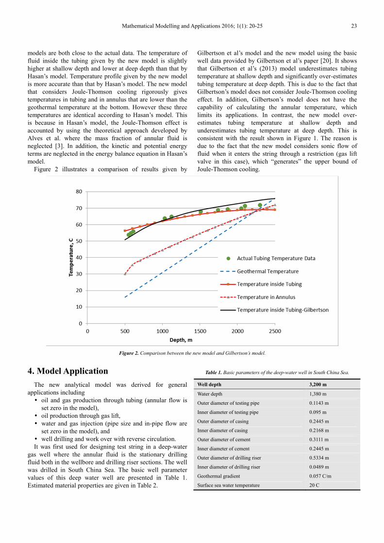
Figure 2 illustrates a comparison of results given by

Gilbertson et al’s model and the new model using the basic

well data provided by Gilbertson et al’s paper [20]. It shows

that Gilbertson et al’s (2013) model underestimates tubing

temperature at shallow depth and significantly over-estimates

tubing temperature at deep depth. This is due to the fact that

Gilbertson’s model does not consider Joule-Thomson cooling

effect. In addition, Gilbertson’s model does not have the

capability of calculating the annular temperature, which

limits its applications. In contrast, the new model over-

estimates tubing temperature at shallow depth and

underestimates tubing temperature at deep depth. This is

consistent with the result shown in Figure 1. The reason is

due to the fact that the new model considers sonic flow of

fluid when it enters the string through a restriction (gas lift

valve in this case), which “generates” the upper bound of

Joule-Thomson cooling.

Figure 2. Comparison between the new model and Gilbertson’s model.

4. Model Application

The new analytical model was derived for general

applications including

� oil and gas production through tubing (annular flow is

set zero in the model),

� oil production through gas lift,

� water and gas injection (pipe size and in-pipe flow are

set zero in the model), and

� well drilling and work over with reverse circulation.

It was first used for designing test string in a deep-water

gas well where the annular fluid is the stationary drilling

fluid both in the wellbore and drilling riser sections. The well

was drilled in South China Sea. The basic well parameter

values of this deep water well are presented in Table 1.

Estimated material properties are given in Table 2.

Table 1. Basic parameters of the deep-water well in South China Sea.

Well depth 3,200 m

Water depth 1,380 m

Outer diameter of testing pipe 0.1143 m

Inner diameter of testing pipe 0.095 m

Outer diameter of casing 0.2445 m

Inner diameter of casing 0.2168 m

Outer diameter of cement 0.3111 m

Inner diameter of cement 0.2445 m

Outer diameter of drilling riser 0.5334 m

Inner diameter of drilling riser 0.0489 m

Geothermal gradient 0.057 C/m

Surface sea water temperature 20 C

24 Boyun Guo and Jinze Song: An Improved Model for Predicting Fluid Temperature in Deep Wells

Table 2. Estimated material properties for the deep-water well in South

China Sea.

Material Density Specific heat Thermal conductivity

(kg/m3) (J/kg-K) (J/(m-K)

Gas 6.5 2,227 0.03

Sea water 1,025 4,180 0.57

Drilling fluid 1,200 1,600 1.75

Steel 7,850 400 43.7

Cement 2,700 600 1.75

Rock 2,640 837 2.25

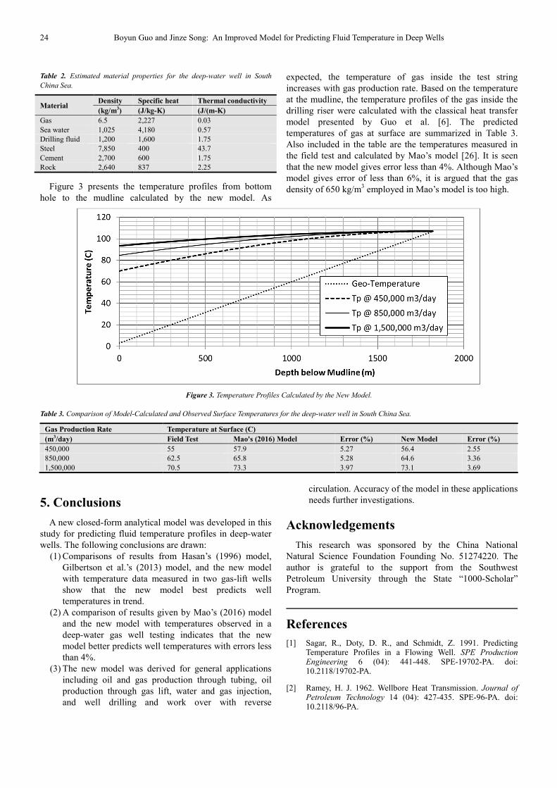
Figure 3 presents the temperature profiles from bottom

hole to the mudline calculated by the new model. As

expected, the temperature of gas inside the test string

increases with gas production rate. Based on the temperature

at the mudline, the temperature profiles of the gas inside the

drilling riser were calculated with the classical heat transfer

model presented by Guo et al. [6]. The predicted

temperatures of gas at surface are summarized in Table 3.

Also included in the table are the temperatures measured in

the field test and calculated by Mao’s model [26]. It is seen

that the new model gives error less than 4%. Although Mao’s

model gives error of less than 6%, it is argued that the gas

density of 650 kg/m3 employed in Mao’s model is too high.

Figure 3. Temperature Profiles Calculated by the New Model.

Table 3. Comparison of Model-Calculated and Observed Surface Temperatures for the deep-water well in South China Sea.

Gas Production Rate Temperature at Surface (C)

(m3/day) Field Test Mao's (2016) Model Error (%) New Model Error (%)

450,000 55 57.9 5.27 56.4 2.55

850,000 62.5 65.8 5.28 64.6 3.36

1,500,000 70.5 73.3 3.97 73.1 3.69

5. Conclusions

A new closed-form analytical model was developed in this

study for predicting fluid temperature profiles in deep-water

wells. The following conclusions are drawn:

(1) Comparisons of results from Hasan’s (1996) model,

Gilbertson et al.’s (2013) model, and the new model

with temperature data measured in two gas-lift wells

show that the new model best predicts well

temperatures in trend.

(2) A comparison of results given by Mao’s (2016) model

and the new model with temperatures observed in a

deep-water gas well testing indicates that the new

model better predicts well temperatures with errors less

than 4%.

(3) The new model was derived for general applications

including oil and gas production through tubing, oil

production through gas lift, water and gas injection,

and well drilling and work over with reverse

circulation. Accuracy of the model in these applications

needs further investigations.

Acknowledgements

This research was sponsored by the China National

Natural Science Foundation Founding No. 51274220. The

author is grateful to the support from the Southwest

Petroleum University through the State “1000-Scholar”

Program.

References

[1] Sagar, R., Doty, D. R., and Schmidt, Z. 1991. Predicting Temperature Profiles in a Flowing Well. SPE Production Engineering 6 (04): 441-448. SPE-19702-PA. doi: 10.2118/19702-PA.

[2] Ramey, H. J. 1962. Wellbore Heat Transmission. Journal of Petroleum Technology 14 (04): 427-435. SPE-96-PA. doi: 10.2118/96-PA.

Mathematical Modelling and Applications 2016; 1(1): 20-25 25

[3] Alves, I. N., Alhanati, F. J. S., & Shoham, O. 1992. A Unified Model for Predicting Flowing Temperature Distribution in Wellbores and Pipelines. Presented at SPE Annual Technical Conference and Exhibition, New Orleans, Louisiana, USA, 23-26 September. SPE- 152039-MS. doi: 10.2118/20632-PA.

[4] Hasan, A. R., and Kabir, C. S. 1994. Aspects of Wellbore Heat Transfer During Two-Phase Flow (includes associated papers 30226 and 30970). SPE Production & Facilities 9 (03): 211-216. SPE-22948-PA. doi: 10.2118/22948-PA.

[5] King, V. P. S., Coelho, L. C., Guigon, J., Cunha, G., and Landau, L. 2005. Analytical Solution for Transient Temperature Field Around a Cased and Cemented Wellbore. Presented at SPE Latin American and Caribbean Petroleum Engineering Conference, Rio de Janeiro, Brazil, 20-23 June. SPE- 94870-MS. doi: 10.2118/94870-MS.

[6] Guo, B., Duan, S., and Ghalambor, A. 2006. A Simple Model for Predicting Heat Loss and Temperature Profiles in Insulated Pipelines. SPE Production & Operations 21 (01): 107-113. doi: 10.2118/86983-PA.

[7] Spindler, R. P. 2011. Analytical Models for Wellbore-Temperature Distribution. SPE Journal 16 (01): 125-133. SPE-140135-PA. doi: 10.2118/140135-PA

[8] Satter, A. 1965. Heat Losses during Flow of Steam down a Wellbore. Journal of Petroleum Technology 17 (07): 845-851. SPE-1071-PA. doi: 10.2118/1071-PA.

[9] Huygen, H. H. A., & Huitt, J. L. 1966. Wellbore Heat Losses and Casing Temperatures during Steam Injection. Presented at Drilling and Production Practice, New York, New York, USA, 1 January. API-66-025.

[10] Back, L. H., and Cuffel, R. F. 1978. Analysis of Heat Losses and Casing Temperatures of Steam Injection Wells with Annular Coolant Water Flow. Presented at SPE California Regional Meeting, San Francisco, California, USA, 12-14 April. SPE- 7148-MS. doi: 10.2118/7148-MS.

[11] Durrant, A. J., and Thambynayagam, R. K. M. 1986. Wellbore Heat Transmission and Pressure Drop for Steam/Water Injection and Geothermal Production: A Simple Solution Technique. SPE Reservoir Engineering 1 (02): 148-162. SPE-12939-PA. doi: 10.2118/12939-PA.

[12] Pacheco, E. F., & Ali, S. M. F. 1972. Wellbore Heat Losses and Pressure Drop In Steam Injection. Journal of Petroleum Technology 24 (02): 139-144. SPE-3428-PA. doi: 10.2118/3428-PA.

[13] Chiu, K., and Thakur, S. C. 1991. Modeling of Wellbore Heat Losses in Directional Wells under Changing Injection Conditions. Presented at SPE Annual Technical Conference and Exhibition, Dallas, Texas, USA, 6-9 October. SPE- 22870-MS. doi: 10.2118/22870-MS.

[14] Kirkpatrick, C. V. 1959. Advances in Gas-lift Technology. Presented at Drilling and Production Practice, New York, New York, USA, 1 January. API-59-024.

[15] Winkler, H. W., and Eads, P. T. 1989. Algorithm for More Accurately Predicting Nitrogen-Charged Gas-Lift Valve Operation at High Pressures and Temperatures. Presented at SPE Production Operations Symposium, Oklahoma City, Oklahoma, USA, 13-14 March. SPE- 18871-MS. doi: 10.2118/18871-MS.

[16] Lagerlef, D. L., Smalstig, W. H., and Erwin, M. D. 1992. Gas-Lift-Valve Test Rack Opening Design Methodology for Extreme Kickoff Temperature Conditions. Presented at SPE Western Regional Meeting, Bakersfield, California, USA, 30 March-1 April. SPE- 24065-MS. doi: 10.2118/24065-MS.

[17] Hasan, A. R., and Kabir, C. S. 1996. A Mechanistic Model for Computing Fluid Temperature Profiles in Gas-Lift Wells. SPE Production & Facilities 11 (03): 179-185. SPE-26098-PA. doi: 10.2118/26098-PA.

[18] Hernandez, A., Garcia, G., Concho, A. M., Garcia, R., and Navarro, U. 1998. Downhole Pressure and Temperature Survey Analysis for Wells on Intermittent Gas Lift. Society of Petroleum Engineers. doi: 10.2118/39853-MS.

[19] Yu, Y., Lin, T., Xie, H., Guan, Y., and Li, K. 2009. Prediction of Wellbore Temperature Profiles During Heavy Oil Production Assisted With Light Oil Lift. Presented at SPE Production and Operations Symposium, Oklahoma, USA, 4-8 April. SPE- 119526-MS. doi: 10.2118/119526-MS.

[20] Gilbertson, E., Hover, F., and Freeman, B. 2013. A Thermally Actuated Gas-Lift Safety Valve. SPE Production & Operations 28 (01): 77-84. SPE-161930-PA. doi: 10.2118/161930-PA.

[21] Han, G., Ling, K., and Zhang, Z. 2014. A Transient Two-Phase Fluid- and Heat-Flow Model for Gas-Lift-Assisted Waxy-Crude Wells with Periodical Electric Heating. Presented at SPE Heavy Oil Conference-Canada, Calgary, Alberta, Canada, 11-13 June. SPE-165415-MS. doi: 10.2118/165415-MS.

[22] Wooley, G. R. 1980. Computing Downhole Temperatures in Circulation, Injection, and Production Wells. Journal of Petroleum Technology 32 (09): 1509 – 1522. SPE-8441-PA. doi: 10.2118/8441-PA.

[23] Leutwyler, K. 1966. Casing Temperature Studies in Steam Injection Wells. Journal of Petroleum Technology 18 (09): 1,157 - 1,162. SPE- 1264-PA. doi: 10.2118/1264-PA.

[24] Tragesser, A. F., Crawford, P. B., & Crawford, H. R. 1967. A Method for Calculating Circulating Temperatures. Journal of Petroleum Technology 19 (11): 1,507-1,512. SPE-1484-PA. doi: 10.2118/1484-PA.

[25] Nelson, W. C. 1977. Circulating Temperatures Existing Prior To Cementing Casing In Prudhoe Bay Wells. Presented at SPE Annual Fall Technical Conference and Exhibition, Denver, Colorado, USA, 9-12 October. SPE- 6802-MS. doi: 10.2118/6802-MS.

[26] Mao, J. and Liu, Q. (2016). Temperature prediction model of gas wells for deep-water testing in South China Sea. Personal communication, JNGSE-D-16-0101.