an improved fuzzy neural network based on t–s model

Available online at www.sciencedirect.com

www.elsevier.com/locate/eswa

Expert Systems with Applications 34 (2008) 2905–2920

Expert Systemswith Applications

An improved fuzzy neural network based on T–S model

Min Han *, Yannan Sun, Yingnan Fan

School of Electronics and Information Engineering, Dalian University of Technology, Linggong Road 2,

Ganjingzi District, Liaoning, Dalian 116023, China

Abstract

An improved fuzzy neural network based on Takagi–Sugeno (T–S) model is proposed in this paper. According to characteristics ofsamples spatial distribution the number of linguistic values of every input and the means and deviations of corresponding membershipfunctions are determined. So the reasonable fuzzy space partition is got. Further a subtractive clustering algorithm is used to derive clus-ter centers from samples. With the parameters of linguistic values the cluster centers are fuzzified to get a more concise rule set withimportance for every rule. Thus redundant rules in the fuzzy space are deleted. Then antecedent parts of all rules determine how a fuzz-ification layer and an inference layer connect. Next, weights of the defuzzification layer are initialized by a least square algorithm. Afterthe network is built, a hybrid method combining a gradient descent algorithm and a least square algorithm is applied to tune the para-meters in it. Simultaneous, an adaptive learning rate which is identified from input-state stability theory is adopted to insure stability ofthe network. The improved T–S fuzzy neural network (ITSFNN) has a compact structure, high training speed, good simulation preci-sion, and generalization ability. To evaluate the performance of the ITSFNN, we experiment with two nonlinear examples. A compar-ative analysis reveals the proposed T–S fuzzy neural network exhibits a higher accuracy and better generalization ability than ordinaryT–S fuzzy neural network. Finally, it is applied to predict markup percent of the construction bidding system and has a better predictioncapability in comparison to some previous models.� 2007 Published by Elsevier Ltd.

Keywords: Takagi–Sugeno model; Fuzzy neural network; Fuzzy space; Rule set

1. Introduction

Fuzzy systems are good at processing the vague anduncertainty information and provide clear advantages inknowledge acquisition but have poor learning ability, whilea neural network has good learning abilities but is not suit-able for expressing rule-based knowledge. Neural networkis usually called a black-box for it is difficult to verify whatthe network has learned so that the users cannot make adecision. Fuzzy logic and artificial neural network havesome similar properties. Both of them may be able tomap the typical nonlinear relation of the input–outputwithout a precise mathematical formula or model betweenthe input and output variables. Functionally, a fuzzy sys-

0957-4174/$ - see front matter � 2007 Published by Elsevier Ltd.

doi:10.1016/j.eswa.2007.05.020

* Corresponding author. Tel.: +86 411 84707847/84708719; fax: +86 41184707847.

E-mail address: [email protected] (M. Han).

tem or a neural network can be described as a functionapproximator. More specifically, they aim at obtaining anapproximation of an unknown mapping f : Rr ! Rs fromsample patterns drawn from the function f (Wu & Er,2000). Theoretical investigations have revealed that neuralnetworks and fuzzy inference systems are universal approx-imators, i.e., they can approximate any function to any pre-scribed accuracy provided that sufficient hidden neurons orfuzzy rules are available. Fuzzy neural network capturesthe advantages of both fuzzy logic and neural networkand discards their weakness. The black-box nature of theneural-network paradigm is resolved, as the connectioniststructure of a fuzzy neural network essentially defines theIF-THEN fuzzy rules (Tung & Quek, 2002). Moreover, afuzzy neural network can self-adjust the parameters offuzzy rules using neural network based learning algo-rithms. So it has been widely used in many fields, such ascontrol, pattern recognition, fault diagnosis and etc.

mailto:[email protected]

2906 M. Han et al. / Expert Systems with Applications 34 (2008) 2905–2920

According to combination ways of fuzzy logic and neu-ral network, fuzzy neural networks are classified into twotypes. The first type is neural networks incorporating somefuzzy logic or fuzzy mathematic operation (Bortolan &Pedrycz, 2002; Ishibuchi & Nii, 2001; Li, Kevman, & Ichik-awa, 2002). The second type is neural networks based onfuzzy inference (Oh, Pedrycz, & Park, 2003; Lin, Yeh,Liang, Chung, & Kumar, 2006; Plamen & Dimitar,2004). The neural networks based on fuzzy inference arepaid more attention. They include fuzzy neural networksbased on Mamdani model and T–S model. As Mamdanimodel the consequent parts of rules are a fuzzy set. Whileas T–S model the consequent parts of rules are functions ofinputs, usually linear one is adopted as a function. Themain advantage of T–S model is to simulate the complexnonlinear system with fewer rules. For its defuzzificationprocess is simpler than Mamdani model it is studied moreuniversally. Recently many studies concentrate on newalgorithms adjusting the weights of fuzzification anddefuzzification layer. Oh, Pedrycz, and Park (2005), Oh,Pedrycz, and Park (2006) proposed a fuzzy polynomialneural network. In fact it was some type of T–S fuzzy neu-ral network. The difference with ordinary T–S fuzzy neuralnetwork was inputs of consequent network may be parts ofinputs. The antecedent network was same to the ordinaryT–S fuzzy neural network. The linguistic values of inputswere set 2 or 3. The number of rules was determined bythe number of inputs and the linguistic values of everyinput. Oh et al. used genetic algorithm to select the conse-quent parameters for the fuzzy polynomial neural network.Because the complexity of the genetic algorithm, more rulesor more outputs will induce large computation cost. Ouy-ang, Lee, and Lee (2005) used the method constructed bythemselves to extract cluster centers, then translated theminto rules. The number of linguistic values of every inputwas same to the number of centers, i.e. means of member-ship functions. More rules, more linguistic values of everyinput. Thus it increased computation cost and the linguisticvalues lost actual meaning. Lin and Xu (2006) built T–Sneural network with consequent parts as constants. Theparameters of membership functions and consequent partof the network were coded and an improved genetic algo-rithm was used to search for the optimum parameters.Tang, Quek, and Ng (2005) proposed T–S network withconsequent part as a linear function of inputs. He also useda genetic algorithm to adjust the parameters. For aboveT–S fuzzy neural networks, in the space partition methodsspace distribution of samples is not considered. The num-ber of linguistic values was determined by experts or users.Means and deviations were determined only by the Min–Max value of samples while the density of samples distribu-tion is not considered. Rules would increase in exponentwith the number of inputs increasing. Hence it aggravatedthe computation burden.

For solving above shortcomings, an improved T–Smodel fuzzy neural network (ITSFNN) is proposed includ-ing structure identification and parameter learning. Fuzzy

space partition process, i.e. antecedent parameters of net-work determination, may automatically run according tothe samples distribution characteristics so that the spaceis partitioned reasonably. A subtractive cluster algorithmis utilized to get kernel rules and an importance of everyrule, removing the redundant rules in fuzzy space. Andthen according to antecedent parts of the rules connectthe fuzzification layer and the inference layer. Thus it sim-plifies the network structure. The parameters of defuzzifi-cation layer are initialized by a least square estimationalgorithm. To refine parameters a hybrid method of thegradient descent algorithm and the least square estimationalgorithm is used to train the network with an adaptivelearning rate. The organization of this paper is as follows.Sections 2 and 3 describe respectively the structure of thenetwork and the learning algorithm. In Section 4 twoexamples are simulated by ordinary T–S fuzzy neuralnetwork (OTSFNN) and the improved T–S fuzzy neuralnetwork. After ITSFNN is verified the ITSFNN is appliedto predict bidding markup percent of construction and iscompared with other fuzzy neural networks in Section 5.

2. Architecture of the ITSFNN

2.1. Takagi–Sugeno model

Let x = [x1,x2, . . . ,xn]T denotes input vector, every vari-able xi is fuzzy linguistic variable. The set of linguistic vari-ables is represented by T ðxiÞ ¼ fA1

i ;A2i ; . . . ;Ami

i g, i =1,2, . . . ,n, where Asi

i ðsi ¼ 1; 2; . . . ;miÞ is the sith linguisticvalue of the input xi. The membership function of fuzzyset defined on domain of xi is lA

siiðxiÞ. Let y =

[y1,y2, . . . ,yr]T denotes output vector. A rule takes form of

Rj : IF x1 is Ajs11 ; x2 is A2js2 ; . . . ; xn is Ajsn

n ; THEN

yj1 ¼ p1j1x1 þ p1

j2x2 þ � � � þ p1jnxn þ p1

jðnþ1Þ;

..

.

yjr ¼ prj1x1 þ pr

j2x2 þ � � � þ prjnxn þ pr

jðnþ1Þ;

where j = 1,2, . . . ,m, m 6Qn

i¼1mi.The degree the input vector x matches rule Rj is com-

puted by the min operator: aj ¼ lA

js11

ðx1Þ ^ lA

js22

ðx2Þ ^ . . .^lAjsn

nðxnÞ or the product operator: aj ¼ l

Ajs11

ðx1Þ�l

Ajs22

ðx2Þ . . . lAjsnnðxnÞ and is called the firing strength of rule

Rj. Suppose the importance of every rule is also knownwj (wj P 1). So output of fuzzy system is weighted averageof outputs of all rules.

yk ¼Pm

j¼1wjajyjkPmj¼1wjaj

; k ¼ 1; . . . ; r: ð1Þ

2.2. Structure of the ITSFNN

The network structure is shown in Fig. 1 based on theabove fuzzy inference process. Fuzzification layer and

Fig. 1. Structure of the ITSFNN.

M. Han et al. / Expert Systems with Applications 34 (2008) 2905–2920 2907

inference layer compose the antecedent network which cor-responds to the ‘‘IF’’ parts of rules. Consequent networkconsists of defuzzification layer corresponding to the‘‘THEN’’ parts of rules. Function of every layer isdescribed as follows.

Fuzzification layer: Input data are fuzzified and member-ships that they belong to every linguistic value are got.Gaussian function is adopted to be membership function.The ith input has mi linguistic values and their meansand deviations of membership functions denoted byðcsii; rsiiÞ, i = 1,2, . . . ,n; si = 1,2, . . . ,mi. So the membershipfunction of the sith linguistic variable for the ith input is

lAsiiðxi; csii; rsiiÞ ¼ exp�ðxi � csiiÞ

2

2r2sii

: ð2Þ

Inference layer: Firing strength of every rule is calculated.There are m rules. According to the premise parts of rules

the neuron representing some linguistic value of some inputis connected with the neuron representing some rule. Forthe rule Rj, we can get the firing strength aj ¼ l

Ajs11

ðx1Þl

Ajs22

ðx2Þ . . . lAjsnnðxnÞ. If importance is known as wj, fir-

ing strength of the rule may be corrected. Then a new firingstrength is got with /j = aj Æ wj. To normalize firing strengthof all rules to [0,1] we can get

�/j ¼/jPmj¼1/j

; j ¼ 1; 2; . . . ;m: ð3Þ

Defuzzification layer: For output yk, outputs of m rules arewk = [wk1,wk2, . . . ,wkm]T, wk ¼ P k~x. The output

yk ¼ /T wk ¼ /T P k~x: ð4Þ

where / ¼ ½�/1; �/2; � � � ; �/m�T , P k ¼pk

11 � � � pk1ðnþ1Þ

. ..

pkm1 � � � pk

mðnþ1Þ

264375,

~x ¼ ½x1; . . . ; xn; xnþ1�T , here xn+1 = 1.


2.3. Fuzzy space partition

Reasonable fuzzy space partition will not only containmore information but also produce fewer rules. A processof partitioning fuzzy space is the premise for constructinga fuzzy neural network. By the traditional method thenumber of linguistic values of every input is given andMin–Max algorithm is used to decide the mean and devia-tion of every membership function. In this traditionalmethod information hidden in data is not used enough.In the paper, according to the distribution density of everyinput and the golden partition algorithm, the number oflinguistic values of inputs and the means and deviationsof the membership functions responding to linguistic valuesare determined.

First a fuzzy space is formed. Each universe Di =[xi,min,xi,max], i = 1,2, . . . ,n is discretized by formulating aset Di of pi > 1 points uniformly distributed along Di.

Di ¼ fdij 2 Dijj ¼ 1; 2; . . . pig;dij ¼ xi;min þ ðj� 1Þðxi;max � xi;minÞ=ðpi � 1Þ; ð5Þ

where pi is an integer representing the discretization accu-racy. The overall set D ¼ D1 � D2 � � � � � Dn defines a gridnetwork over the space D = D1 · D2 · � � � · Dn. Supposethe set Li comprising all possible crisp intervals lr

i uniquelydefined over Di : Li ¼ flw

i ¼ ðuwi ; v

wi Þjuw

i ; vwi 2 Di; uw

i < vwi ;

w ¼ 1; 2; . . . ; cardðLiÞ ¼ piðpi � 1Þ=2g, where uwi and vw

i arethe starting and ending point of the interval lw

i and card(Li)is the cardinal number of Li determined by pi. For eachcrisp interval lw

i 2 Li; i ¼ 1; 2; . . . ; n the responding fuzzy

set is denoted by ~lwi ¼ fðxi; f w

i ðxiÞÞjxi 2 Dig. The member-ship function is Gaussian function and is given by

f wi ðxiÞ ¼ exp� ðxi�cw

i Þ2

2ðrwi Þ

2 , where cwi ¼ ðuw

i þ vwi Þ=2 is the mean

of the membership function and rwi ¼ ðvw

i � uwi Þ=2 is the

deviation of the function. All sets of ~lwi ðw ¼ 1; 2; . . . ;

cardðLiÞÞ comprise the fuzzy set eLi. There is a one-to-onemapping between the elements of Li and those of eLi.

So the fuzzy space defined on the space D = D1 ·D2 · � � � · Dn would be defined by (Papadakis & Theo-charis, 2002)

eH ¼ eL1� eL2� � � � � eLn

¼ ~hw ¼ ð~lw1 ; � � � ;~lw

n Þjw¼ 1; . . . ; cardð eH Þ ¼Yn

i¼1

cardðLiÞ( )

:

ð6Þ

Some element in the fuzzy space eH consists of n fuzzy sets~ho ¼ ð~lo1

1 ; . . . ;~lonn Þ, ~ho 2 eH , where oi 2 {1,2, . . . , card(Li)}. A

fuzzy set ~ho comprises the antecedent parts of a rule.For input vector x = [x1,x2, . . . ,xn]T the correspondingmembership is ðf o1

1 ðx1Þ; . . . ; f onn ðxnÞÞ. The firing strength

of the rule is a ¼ f o11 ðx1Þ � � � � � f on

n ðxnÞ. In T–S fuzzysystems, some input xi has mi linguistic values, i.e.Asi

i ðsi ¼ 1; 2; . . . ;miÞ. So ~ho ¼ ð~lo11 ; . . . ;~lon

n Þ may be denotedby ~ho ¼ ðAs1

1 ; . . . ;Asnn Þ, si 2 {1,2, . . . ,mi}.

After a fuzzy space is formed, it should be partitioned.Whatever the traditional grid partition and the scatter par-tition they are both based on the above fuzzy space. But forthe traditional partition methods are not proper, the spacepartitioned does not reflect the characteristics of the sam-ples. In the paper all parameters of membership functionsincluding the number of the linguistic values and the corre-sponding means and deviations are all automatically deter-mined based on distribution of the samples that is called‘‘the data distribution method’’. Suppose two variables x1

and x2, there are n patterns. For the variable x1, fuzzifica-tion parameters are determined as follows.

Step one: An initial center vector is obtained by calculat-ing the percent of the data in same value over total data.

Suppose the number of x1 = a is m, labeled by Pera =m/n. Set a threshold Perv. If Pera > Perv, the data value a

is a center or a mean of a membership function. If percentsof all data in different value are less than the threshold, thethreshold is reduced, Perv = 0.8 · Perv. Another thresholdPervmin is given. When Perv < Pervmin or there has beensome centers the process will terminate. The initial centervector is c = [c1,c2, . . . ,cini] ascending ordered by centervalue. If there is no any center, c = (x1,min + x1,max)/2 willbe a center.

Step two: New centers are added by calculating distribu-tion density of the data with different values between twocontiguous centers.

Calculating density of the data with different valuesbetween two contiguous centers in initial center vector,labeled as q = ndif/(cj � ci) j > i, i,j = 1,2, . . . , ini. Averagedistribution density for all different data is qv = ndif/(x1,max � x1,min). If q > qv, it means that the points betweencj and ci are too dense. So a new center between the twocenters is created. According to the golden partitionmethod the new center is determined as c0i ¼ ci þ 0:618�ðcj � ciÞ. If q < qv, it is not necessary to create a new center.New center is created until the density between all twoadjacent centers is less than the threshold qv. The final cen-ter vector is c = [c1, . . . ,ci, . . . ,cfin], ci > ci�1.

Step three: Width is determined.After above two steps the location and the number of

the membership functions are decided. Next is to determinewidths, i.e. deviations, of membership functions. Accord-ing to the golden partition method, the deviation of mem-bership function corresponding to the center is calculatedby r = 0.618 · (dis/2), where dis is the minimum distanceof the center to the adjacent left and right center. Thusoverlapping of two adjacent membership functions is nottoo large so that the linguistic value is nearly single.

There are 70 patterns for variables x1 and x2. For thevariable x1, the data distribution is shown in Fig. 2 withsmall circles. There are six kinds of data with different val-ues. The data with value 0.5 are 37.1% of all data. Usingthe method proposed in the paper the membership func-tions are shown in Fig. 2 with the line. The number ofthe linguistic values are automatically determined as 4.The mean and deviation of the 4 membership functions

Fig. 2. Parameters determination for membership functions by the datadistribution method.


are respectively: (0.42, 0.0247), (0.5,0.0247), (0.58, 0.0247)and (0.9,0.0989). Here Perv = 10%, qv = 7.5. For the vari-able x2, the same method is used to determine the param-eters of linguistic values.

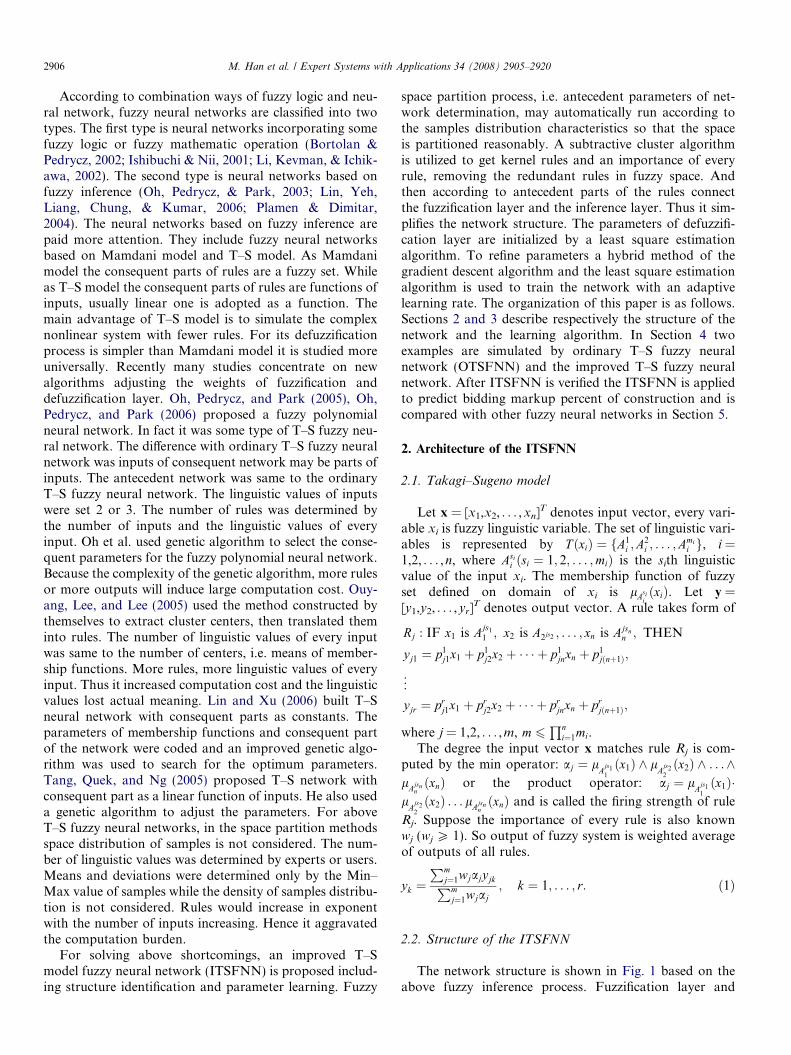
The space built on (x1,x2) is shown in Fig. 3. Circles rep-resent points (x1,x2). Total number of points is 70. Manypoints have the same location so some are overlappingtogether. The partitioned fuzzy space with the Min–Maxmethod to determine the parameters of the membershipfunctions is shown in Fig. 3a. The number of linguistic val-ues of two variables is both set 3. From Fig. 3a the parti-tion of the fuzzy space can not distinguish the differentdata group. Using the method previously described, i.e.the data distribution method, the fuzzy space partition isshown in Fig. 3b. Variable x1 is automatically set 4 linguis-tic values and variable x2 has 2 linguistic values. Differentpoints belong to different space. The fuzzy space inFig. 3b is reasonably partitioned. The partitioned spacewhich represents the distribution characteristics of pointsis the premise for fuzzy inference process.

2.4. Rules extraction

Based on the determined membership functions, thenumber of all the possible rules will be

Qni¼1mi. In those

rules some are redundant. For simplifying the networkstructure, clustering algorithm is used to remove the redun-dant rules. Finally the number of the concise rules is m,m 6

Qni¼1mi. It is not necessary that fuzzification layer

and inference layer are connected completely. For a simpli-fied network the fuzzification layer and the inference layeris connected partly according to antecedent parts of theconcise rules. There are three representative clustering tech-niques: K-means clustering; Fuzzy C-means clustering andSubtractive clustering. Some of the clustering techniquesrely on knowing the number of clusters apriori. In that case

the algorithm tries to partition the data into the given num-ber of clusters. K-means and Fuzzy C-means clustering areof that type. In other cases it is not necessary to have thenumber of clusters known from the beginning; insteadthe algorithm starts by finding the first large cluster, andthen goes to find the second, and so on. Subtractive cluster-ing is of that type. In a problem of known cluster numbersboth types can be applied; however if the number ofclusters is not known, K-means and Fuzzy C-means clus-tering can not be used. In the paper the number of clustersis not known so the subtractive clustering is adopted.First cluster centers are extracted by the subtractive clus-tering algorithm. Then the cluster centers are trans-formed into rules with importance. Last the rules are asneurons in the reference layer of the network. Accordingto the premises of the rules the fuzzification layer and ref-erence layer is connected to build the initial structure of thenetwork.

For a collection of z data points S = {s1, . . . , sz}, si =[xi1,xi2, . . . ,xin,yi1,yi2, . . . ,yir], in (n + r) dimensional space,sik denotes the kth coordinate of the ith data point, wherei = 1,2, . . . ,z and k = 1,2, . . . ,n + r. After normalizing thedata, get the cluster centers by the subtractive clusteringmethod (Chiu, 1994; Tao, 2002; Yager & Filev, 1994).

Each data point is a candidate for cluster centers. A den-sity measure at data point si is defined as

Di ¼Xz

j¼1

exp �ksi � sjk2

krak2=4

!; ð7Þ

where ra ¼ ½r1a; r

2a; . . . ; rnþr

a � represents the neighborhood ra-dius for every data point. For every coordinate of the pointthere is different radius. Points which are out of the neigh-borhood have little effect on the point si. But all points inthe neighborhood will have lager effect on the point thatwill be a center point. Hence a data point si will have a highdensity value if it has many neighborhood points. The datapoint having the largest density value Dc1 will be chosen asthe first cluster center sc1.

Next the density measure of each point si is revised asfollowing equation:

Di ¼ Di � Dc1 exp �ksi � sc1k2

krbk2=4

!; ð8Þ

where rb is a positive constant vector which defines a neigh-borhood that has measurable reductions in density mea-sure. Therefore, the data points near the first clustercenter sc1 will have significantly reduced density measure.For escaping from centers congregating krbk is usuallylarger than krak, for example krbk = 1.5 krak. After revisingthe density function, the next cluster center is selected asthe point having the greatest density value. This processcontinues.

Hypothesize the rth center has been decided. Then thepossibility changed into centers of the residual points

decreased to Di ¼ Di � Dcr exp � ksi�scrk2

krbk=4

� �.

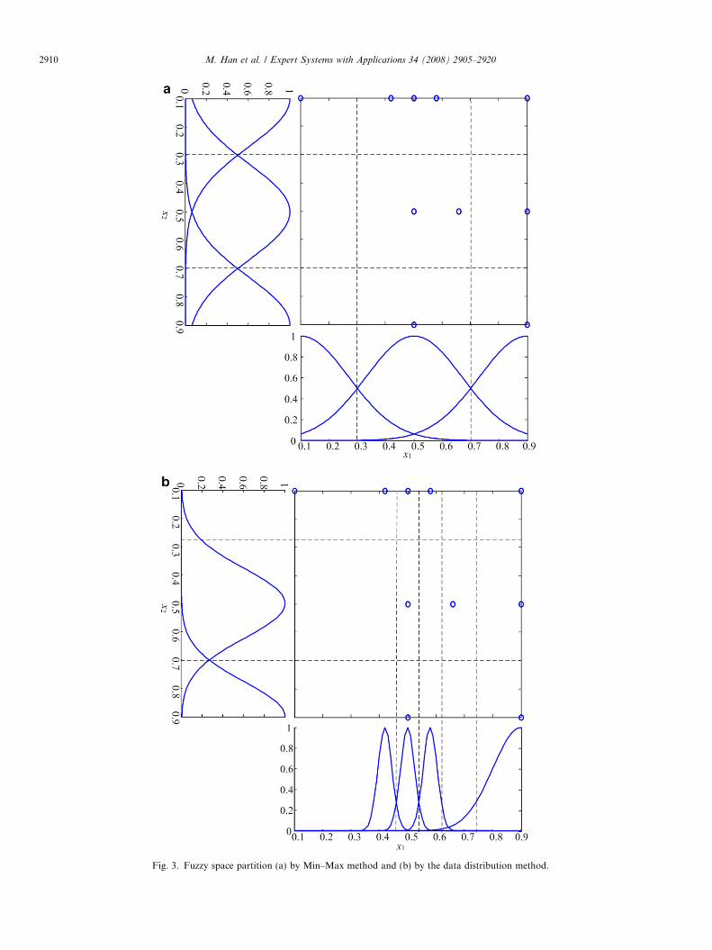
Fig. 3. Fuzzy space partition (a) by Min–Max method and (b) by the data distribution method.



If Dk > �eD1, sk is the next center sck, k = 1,2, . . . , r; �e isa positive constant. If Dk 6 eD1, the process ends.e isalso a positive constant, e < �e. But if eD1 < Dk < �eD1,we have to calculate dmin

krak þDkD1

P 1 (where dmin is the short-est distance between sk and previously found clustercenters). If it is true, sk is selected as a cluster centersck and process continues. Otherwise we set Dk = 0and select the point with next highest density to testthe conditions. At last we attain m 0 cluster centers[sc1,sc2, . . . , scm0].

The centers then are transformed into rules. For T–Smodel a consequent part of a rule is a linear function ofinputs, not a fuzzy linguistic value, so only antecedent partsof rules are enough to determine the structure of the infer-ence layer. First output variables of each cluster center aredeleted. One cluster center can be labeled by sci = [sci1,sci2, . . . ,scin]. Then the centers are fuzzified with member-ship functions of every input decided by the methodahead. For a center sci, scij is fed into the membership func-tions corresponding to the mj linguistic values of the jthinput variable. The linguistic value which has the largestmembership is denoted by Ajmax and it is the fuzzy valueof scij. Further the premise part of a rule Ri correspondingto the center sci is ‘‘IF x1 is A1max, x2 is A2max, . . .,xn isAnmax’’.

A cluster center is transformed into a fuzzy rule with animportance of 1. If a following cluster center is fuzzified tothe same rule, the importance of the rule will increase by0.1, and wipe off this center from center set. This processcontinuous until all the cluster centers are fuzzified com-pletely. At last the rules with importance are obtained.And the concise cluster centers [sc1, sc2, . . . , scm] are formed,too. All rules are represented by nodes in the inferencelayer shown in Fig. 1. According to the premises of rules,the neurons representing rules and the neurons represent-ing the linguistic values corresponding to the rules are con-nected together. For programming conveniently, thelinguistic values of every input in order of means of mem-bership functions are labeled. For example, the input x1

has 3 linguistic values which mean ‘‘small’’, ‘‘middle’’ and‘‘big’’. The number 1 represents ‘‘small’’; 2 means ‘‘middle’’and 3 denotes ‘‘big’’. Suppose there is a 2-input system.Premise of one rule is ‘‘If x1 is 1, x2 is 3’’. Thus the neuronrepresenting the rule will connect neurons representing thefirst linguistic value of x1 and the third linguistic valueof x2.

2.5. Initialization of consequent parameters

If consequent parameters are initialized based on thepriori knowledge, the network will get a lower initial errorthan randomly determining them and will cost less trainingtime. The initial weights of the defuzzification layer may bedetermined by the concise cluster centers and the initialweights of the fuzzification layer. Still suppose z datapoints to form a sample matrix S. Input and output matrixare defined by

X z�ðnþ1Þ ¼

~xT1

..

.

~xTz

26643775; Y z�r ¼

yT1

..

.

yTz

26643775 ð9Þ

The weight matrix of the defuzzification layer correspond-ing to the kth output is denoted by Pk in Eq. (4). Letpk

i ¼ ½pki1; p

ki2; . . . ; pk

iðnþ1Þ�T , Pk is transformed into a column

vector. So a matrix formed by all weights correspondingto r outputs is

P ¼

p11 � � � pr

1

. ..

p1m � � � pr

m

26643775ððnþ1Þm�rÞ

: ð10Þ

A matrix Mz·(n+1)m should be constructed so that MP = Y.All samples are fed into the network shown in Fig. 1.

The output matrix of the inference layer is

U ¼/T

1

..

.

/Tz

26643775 ¼

�/11 � � � �/1m

. ..

�/z1 � � � �/zm

26643775: ð13Þ

According to Eq. (4), we will get the matrix M:

Mi ¼~x1 � �/1i

..

.

~xz � �/zi

26643775; i ¼ 1; 2; . . . ;m:

ð14Þ

By the least square algorithm, P = (MTM)�1MTY. The kthcolumn of matrix P is turned back to matrix Pk. So theweights of the defuziffication layer corresponding to thekth output are obtained.

3. Learning algorithm of ITSFNN

3.1. An adaptive learning rate

For the improved T–S fuzzy neural network, the qthoutput of the model can be expressed by

yq ¼

Pmi¼1

Pnþ1k¼1pq

ik � xk

� �� wiQn

j¼1 exp�ðxj�ci

sjjÞ2

2ðrisjjÞ

2

� �Pm

i¼1wiQn

j¼1 exp�ðxj�ci

sjjÞ2

2ðrisjjÞ

2

;

q ¼ 1; 2; . . . ; r: ð15Þ

ðcisjj; ri

sjjÞ is the mean and deviation of the membershipfunction of the sjth linguistic value of the jth input connect-ing with the neuron representing the ith rule.

Yu and Li (2004) verified that an adaptive learning rateg 0 = g/(1 + kAk2 + 2kBk2) can guarantee the stability oftraining process by the theory of input-to-state stability.For the improved T–S fuzzy neural network, A and B inthe above formula are calculated by


A ¼ / � x1; . . . ;/ � xn; /½ �;

B ¼

a1w1ðw11�y1ÞPm

j¼1ajwj

� � � amwmðw1m�y1ÞPm

j¼1ajwj

..

. ...

a1w1ðwrm�yrÞPm

j¼1ajwj

� � � amwmðwrm�yrÞPm

j¼1ajwj

266664377775: ð16Þ

3.2. A hybrid method refining weights

Though the gradient decent algorithm can be used toidentify the parameters in the network, it is very slowand likely to be trapped into a local minimum. So in thispaper a hybrid algorithm with gradient decent algorithmand least square estimation algorithm is used to train thenetwork. Set interval iterations x as an integer such thatx 2 [5,20]. When the iteration is integer times of x, the leastsquare estimation is applied to adjust the consequentparameters. On the other iterations the gradient descentmethod is used to adjust all the parameters.

Objective function is selected as

e ¼ ð1� RcÞ � 1=2Xr

q¼1

ðy 0q � yqÞ2 þ Rc � 1

2Nx

XNx

i¼1

ðxiÞ2: ð17Þ

y0q is the qth desired output and yq is the qth output of net-work. Rc is a regularization coefficient which is set 0.01 bytrail and error method. xi, i = 1,2, . . . ,Nx represent allparameters to be adjusted.

The adjustment equations of consequent parameters areas follows:

pqjiðt þ 1Þ ¼ pq

jiðtÞ þ Dpqji;

DpqjiðtÞ ¼ ð1� aÞD0pq

jiðtÞ þ aDpqjiðt � 1Þ;

D0pqjiðtÞ ¼

Xz

u¼1

D0pqjiðuÞ;

D0pqjiðuÞ ¼ �g0

oeopq

ji¼ �g0 � oe

oyq

�oyq

owqj

�owqj

opqji

¼ �g0 � ½�ðy 0uq � yuqÞ� � �/j � xui; ð18Þ

where q = 1,2, . . . , r; i = 1,2, . . . ,n + 1; j = 1,2, . . . ,m;u = 1,2, . . . ,z. r is the number of outputs; n is the numberof inputs; z is the number of training samples. The momentcoefficient is a = 0.9. And xn+1 = 1.

The adjustment equations of means of membershipfunctions in the antecedent network are as follows:

csiiðt þ 1Þ ¼ csiiðtÞ þ DcsiiðtÞ;DcsiiðtÞ ¼ ð1� aÞD0csiiðtÞ þ aDcsiiðt � 1Þ;

D0csiiðtÞ ¼Xz

u¼1

D0csiiðuÞ;

DcsiiðuÞ ¼ �g0 �Xm

j¼1

oeoaj� oaj

ocsii¼ �g0 �

Xm

j¼1

Midj � aj �ðxui � csiiÞ

r2sii

;

ð19Þ

where i = 1,2, . . . ,n; si = 1,2, . . . ,mi. mi is the number oflinguistic values of the ith input.

The adjustment formula of deviations of membershipfunctions are shown by following equations:

rsiiðt þ 1Þ ¼ rsiiðtÞ þ DrsiiðtÞ;DrsiiðtÞ ¼ ð1� aÞD0rsiiðtÞ þ aDrsiiðt � 1Þ;

D0rsiiðtÞ ¼Xz

u¼1

D0rsiiðuÞ;

D0rsiiðuÞ ¼ �g0Xm

j¼1

Midj � aj �ðxui � csiiÞ

2

r3sii

: ð20Þ

If the neuron representing the linguistic value of the ithinput which connects with the neuron representing the jthrule is the sith linguistic value. Midj(j = 1,2, . . .,m) is

Midj ¼oeoaj¼Xr

q¼1

oeoyq

�oyq

oaj

¼Xr

q¼1

�ðy 0q � yqÞ �wjðwqj � yqÞPm

j¼1aj � wj: ð21Þ

Otherwise, Midj = 0.When the iteration is integer times of x, fix the premise

parameters, the consequence network can be representedby a matrix equation MP = Y, where M, just likeEq. (14), is denoted by

Mz�ðnþ1Þm ¼

mT1

..

.

mTz

26643775: ð22Þ

Y and P are represented by Eqs. (9) and (10). P is estimatedas P* by the least square algorithm:

P iþ1 ¼ P i þ Biþ1miþ1ðyTiþ1 �mT

iþ1P iÞ;

Biþ1 ¼ Bi �Bimiþ1mT

iþ1Bi

1þmTiþ1

Bimiþ1; i ¼ 0; 1; . . . ; z:

ð23Þ

P* = Pz. Initial condition is P0 = 0, B0 = cI, c is usually abigger constant, here it is 300, I is a (n + 1)m unit matrix.

In this paper the root mean square error (RMSE) oftraining samples and testing samples are calculated respec-tively to evaluate the ability of the network:

RMSE ¼

ffiffiffiffiffiffiffiffiffiffiffiffiffiffiffiffiffiffiffiffiffiffiffiffiffiffiffiffiffiffiffiffiffiffiffiffiffiffiffiffiffiffiffiffiffiffiffiffiffiffi1

N � r

XN

i¼1

Xr

q¼1

ðy0iq � yiqÞ2

vuut ; ð24Þ

where N is the number of training samples or testingsamples.

4. Two simulation examples

4.1. Example 1

A nonlinear example with 3 inputs and a single output isdefined by


y ¼ ð1þ x0:51 þ x�1

2 þ x�1:53 Þ2: ð25Þ

The system output y is highly nonlinear with respect to in-put x1, x2 and x3. We generate a group data of 341 points,with the inputs selected on the domain [1,6] · [1,6] · [1, 6]in which 300 samples are used to train the network. Twonetworks, the improved T–S fuzzy neural network (ITS-FNN) and the ordinary T–S fuzzy neural network (OTS-FNN), are respectively applied to approach the function.Training error and testing error curves for ITSFNN areshown in Fig. 4a. In Fig. 4b comparison between desired

Fig. 4. Simulation results of ITSFNN (a) error curves and

output and ITSFNN output is shown (upper subfigure)and absolute error is shown (lower subfigure). OTSFNNis trained to get the training and testing error graphs(Fig. 5a). Then comparison and absolute error are shownin Fig. 5b. Determined parameters and final RMSE oftwo networks are listed in Table 1.

For the ITSFNN, the number of linguistic values ofevery input is respective 9, 11 and 11 determined by thedata distribution method. There may be 1089 rules. Butafter subtractive clustering, the real number of rules is300. The adaptive learning rate will guarantee the stability

(b) comparison of desired output and network output.

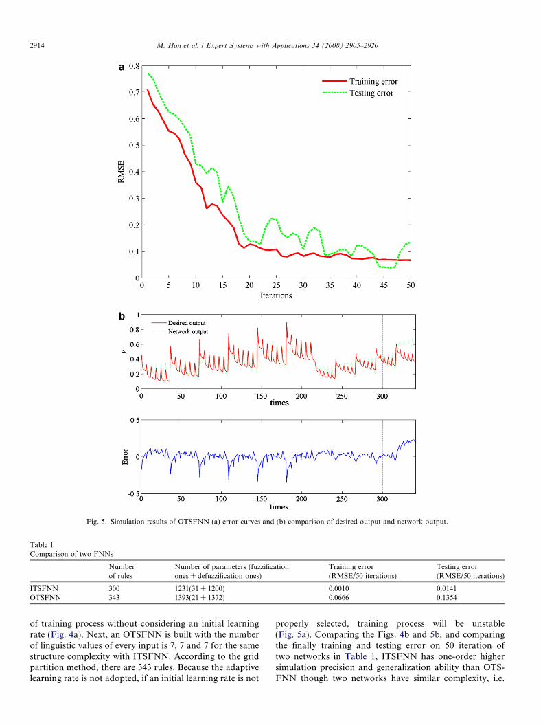
Fig. 5. Simulation results of OTSFNN (a) error curves and (b) comparison of desired output and network output.

Table 1Comparison of two FNNs

Numberof rules

Number of parameters (fuzzificationones + defuzzification ones)

Training error(RMSE/50 iterations)

Testing error(RMSE/50 iterations)

ITSFNN 300 1231(31 + 1200) 0.0010 0.0141OTSFNN 343 1393(21 + 1372) 0.0666 0.1354


of training process without considering an initial learningrate (Fig. 4a). Next, an OTSFNN is built with the numberof linguistic values of every input is 7, 7 and 7 for the samestructure complexity with ITSFNN. According to the gridpartition method, there are 343 rules. Because the adaptivelearning rate is not adopted, if an initial learning rate is not

properly selected, training process will be unstable(Fig. 5a). Comparing the Figs. 4b and 5b, and comparingthe finally training and testing error on 50 iteration oftwo networks in Table 1, ITSFNN has one-order highersimulation precision and generalization ability than OTS-FNN though two networks have similar complexity, i.e.


the number of rules and the number of parameters of OTS-FNN are close to ones of ITSFNN.

An initial error of networks has a strong relation withinitial parameters of fuzzification layer and defuzzifica-tion layer. Consider three ways of determining initialparameters.

(1) Fuzzification parameters are heuristic. The numberof linguistic values is decided by experience. Meansand deviations are determined by Min–Max method.Defuzzification parameters are randomly created.The OTSFNN adopts this way. Under this condition,initial error is mainly affected by the following fac-tors: the number of linguistic values of every input;means and deviations of membership functions; ran-dom defuzzification parameters.

(2) Fuzzification parameters are determined according toexperts’ experience, but defuzzification parametersare determined by a least square algorithm. Thus ini-tial error is determined by the number of linguisticvalues of every input; mean and deviation of member-ship functions and the radius vector in the subtractiveclustering process.

(3) Not only fuzzification parameters are determined bythe data distribution method but also defuzzificationparameters are decided by a least square algorithm.The ITSFNN adopts this way. Now initial error ismainly affected by the two thresholds in the determi-nation process of fuzzification parameters and theradius vector in the subtractive clustering process.

In three different conditions, different factors are calcu-lated to get 10 times of initial error of the network, andthen average the errors. The average errors of three waysare shown in Table 2 from which it is clear that initial errorunder the first way is largest. It is 0.6546. When consequentparameters are determined by a least square algorithm andpremise parameters are determined by experience, RMSEdecreases by 9/10 of the error under the first way (the sec-ond way in Table 2). The third way adopts the method inthe paper, i.e. antecedent parameters decided by the datadistribution method and consequent parameters aredecided by a least square algorithm. Now RMSE decreasesto the 1/10 of the error under the second way. It is 0.0091.So adopting the method of determining fuzzification anddefuzzification parameters in this paper the lowest initialerror is attained.

OTSFNN and ITSFNN in the paper use different waysto determine the parameters of the membership functions.Premise parameters in ITSFNN are decided by the data

Table 2Initial RMSE of training samples comparison for different ways ofdetermining parameters

The first way The second way The third way

Average RMSE 0.6546 0.0767 0.0091

distribution method. For the same complexity with ITS-FNN, the number of linguistic values of 3 inputs of OTS-FNN is 7 and the means and deviations of membershipfunctions are determined by Min–Max method. The mem-bership functions of every input in two networks are shownin Fig. 6. Dashed line describes membership functions byMin–Max method in OTSFNN while solid line meansthe automatically determined membership functions inITSFNN.

Some rules abstracted from ITSFNN are as follows:

Rule 1: IF x1 is l(0.7360,0.0492), x2 is l (0.4177,0.0246),x3 is l(0.5769,0.0246) THENy is 0.1359x1 + 0.0770x2 + 0.1068x3 + 0.1845;Rule 2: IF x1 is l(0.0994,0.0245), x2 is l (0.2586,0.0246),x3 is l(0.4177,0.0246) THENy is 0.0139x1 + 0.0355x2 + 0.0574x3 + 0.1368;Rule 3: IF x1 is l(0.4177,0.0247), x2 is l (0.8951,0.0246),x3 is l(0.4177,0.0246) THENy is 0.0479x1 + 0.1026x2 + 0.0479x3 + 0.1142;Rule 4: IF x1 is l(0.5762,0.0488), x2 is l (0.8951,0.0246),x3 is l(0.8951,0.0246) THENy is 0.0542x1 + 0.0841x2 + 0.0841x3 + 0.0936;Rule 5: IF x1 is l(0.1793,0.0244), x2 is l(0.1796,0.0242),x3 is l(0.3392,0.0246) THENy is 0.0392x1 + 0.0390x2 + 0.0739x3 + 0.2176,

where l(c,r) is the linguistic value corresponding to themembership function whose mean is c and deviation is r.

4.2. Example 2

Consider a nonlinear system:

z ¼ sin x sin yxy

: ð26Þ

It produces a group of input-output data of 600, with x andy 2 [�10,10]. Four hundred patterns are used to train thenetwork and others for testing the generalization abilityof the network.

In Table 3 TSFNN1 is the ITSFNN in the paper. Thenumber of linguistic values of every input is 20. Mem-bership functions are automatically determined. Clustercenters obtained by subtractive cluster algorithm are fuzzi-fied and rules with same antecedent parts are merged to getthe importance of each rule. Finally 274 rules are obtained.At the same time consequent parameters are decided by aleast square algorithm. When iteration is 50th, trainingerror is 0.0090 and testing error is 0.0099. In TSFNN2,the numbers of linguistic values of two inputs are set 11.Means and deviations of membership functions are gotby Min–Max method. But 81 rules are extracted by themethod in the paper and the way how connect the fuzzifi-cation layer and the inference layer is same to ITSFNN.And the consequent parameters are decided by the methodin the paper. Finally we get RMSE of training error 0.0228and testing error 0.0228 that are about 10 times of the

Fig. 6. Membership functions of the three inputs in two NNs.

Table 3Comparison of three NNs

Numberof rules

Number of parameters(antecedent ones +consequent ones)

Training error(RMSE)

Testing error(RMSE)

TSFNN1 274 862(40 + 822) 0.0090/50 iteration 0.0099/50 iterationTSFNN2 81 265(22 + 243) 0.0228/50 iteration 0.0228/50 iterationTSFNN3 400 1240(40 + 1200) 0.0848/200 iteration 0.1295/200 iteration


errors of TSFNN1. TSFNN3 is an ordinary T–S fuzzy neu-ral network. Twenty linguistic values for every input areselected for the number is same to TSFNN1. The numberof rules will be 20 · 20 = 400. Consequent parameters arerandomly produced. Even it is trained for 200 iterations,it has larger training and testing error. Fig. 7b–d are thefunction surfaces reconstructed by outputs of three typesof TSFNNs in Table 3. Fig. 7a is the initial function sur-face. It is clear that the method proposed by this papercan reconstruct function surface more accurately.

5. Construction bidding markup calculation using ITSFNN

The optimum bid markup, defined herein as the ratio ofthe bid over the estimated project cost, is obtained by con-sidering the product of the probability of winning, timesthe expected profit, which maximizes the expected value(Christodoulou, 2004). Construction bidding is a very com-plex decision requiring simultaneous assessment of a largenumber of highly interrelated variables to arrive at a deci-sion (Chua, Li, & Chan, 2001), and estimating the markup

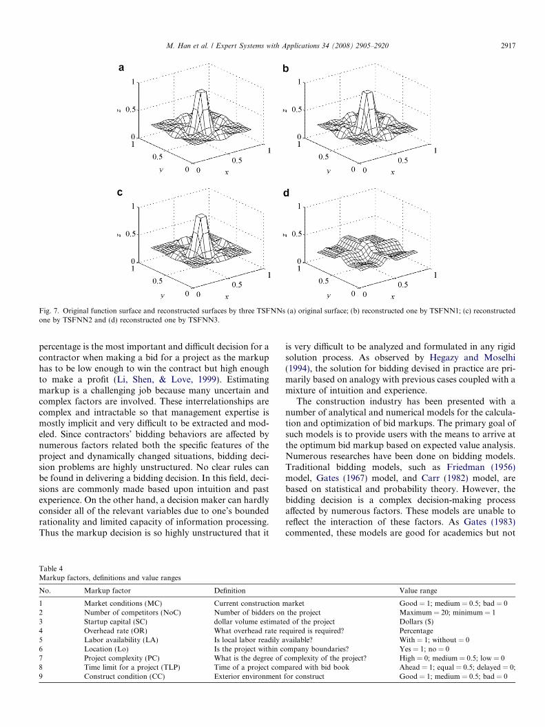
Fig. 7. Original function surface and reconstructed surfaces by three TSFNNs (a) original surface; (b) reconstructed one by TSFNN1; (c) reconstructedone by TSFNN2 and (d) reconstructed one by TSFNN3.


percentage is the most important and difficult decision for acontractor when making a bid for a project as the markuphas to be low enough to win the contract but high enoughto make a profit (Li, Shen, & Love, 1999). Estimatingmarkup is a challenging job because many uncertain andcomplex factors are involved. These interrelationships arecomplex and intractable so that management expertise ismostly implicit and very difficult to be extracted and mod-eled. Since contractors’ bidding behaviors are affected bynumerous factors related both the specific features of theproject and dynamically changed situations, bidding deci-sion problems are highly unstructured. No clear rules canbe found in delivering a bidding decision. In this field, deci-sions are commonly made based upon intuition and pastexperience. On the other hand, a decision maker can hardlyconsider all of the relevant variables due to one’s boundedrationality and limited capacity of information processing.Thus the markup decision is so highly unstructured that it

Table 4Markup factors, definitions and value ranges

No. Markup factor Definition

1 Market conditions (MC) Current construction m2 Number of competitors (NoC) Number of bidders on3 Startup capital (SC) dollar volume estimate4 Overhead rate (OR) What overhead rate re5 Labor availability (LA) Is local labor readily a6 Location (Lo) Is the project within c7 Project complexity (PC) What is the degree of8 Time limit for a project (TLP) Time of a project com9 Construct condition (CC) Exterior environment

is very difficult to be analyzed and formulated in any rigidsolution process. As observed by Hegazy and Moselhi(1994), the solution for bidding devised in practice are pri-marily based on analogy with previous cases coupled with amixture of intuition and experience.

The construction industry has been presented with anumber of analytical and numerical models for the calcula-tion and optimization of bid markups. The primary goal ofsuch models is to provide users with the means to arrive atthe optimum bid markup based on expected value analysis.Numerous researches have been done on bidding models.Traditional bidding models, such as Friedman (1956)model, Gates (1967) model, and Carr (1982) model, arebased on statistical and probability theory. However, thebidding decision is a complex decision-making processaffected by numerous factors. These models are unable toreflect the interaction of these factors. As Gates (1983)commented, these models are good for academics but not

Value range

arket Good = 1; medium = 0.5; bad = 0the project Maximum = 20; minimum = 1d of the project Dollars ($)quired is required? Percentagevailable? With = 1; without = 0

ompany boundaries? Yes = 1; no = 0complexity of the project? High = 0; medium = 0.5; low = 0pared with bid book Ahead = 1; equal = 0.5; delayed = 0;for construct Good = 1; medium = 0.5; bad = 0


for practitioners. Recently, some bidding decision supportsystems based on the artificial intelligence (AI) technique

Table 5Parts of input-output data (ten samples)

Input MC NoC SC OR L

1 0.5 4 0.1000 3.7 02 0.0 9 0.0873 6.3 13 1.0 7 0.0726 4.5 04 0.5 6 0.0781 5.0 05 1.0 4 0.0388 5.2 16 0.5 5 0.1140 6.3 17 1.0 8 0.0510 4.2 08 1.0 6 0.0760 5.2 19 0.5 7 0.0897 4.8 0

10 1.0 5 0.0871 4.7 0. . . . . . . . . . . . . . . .

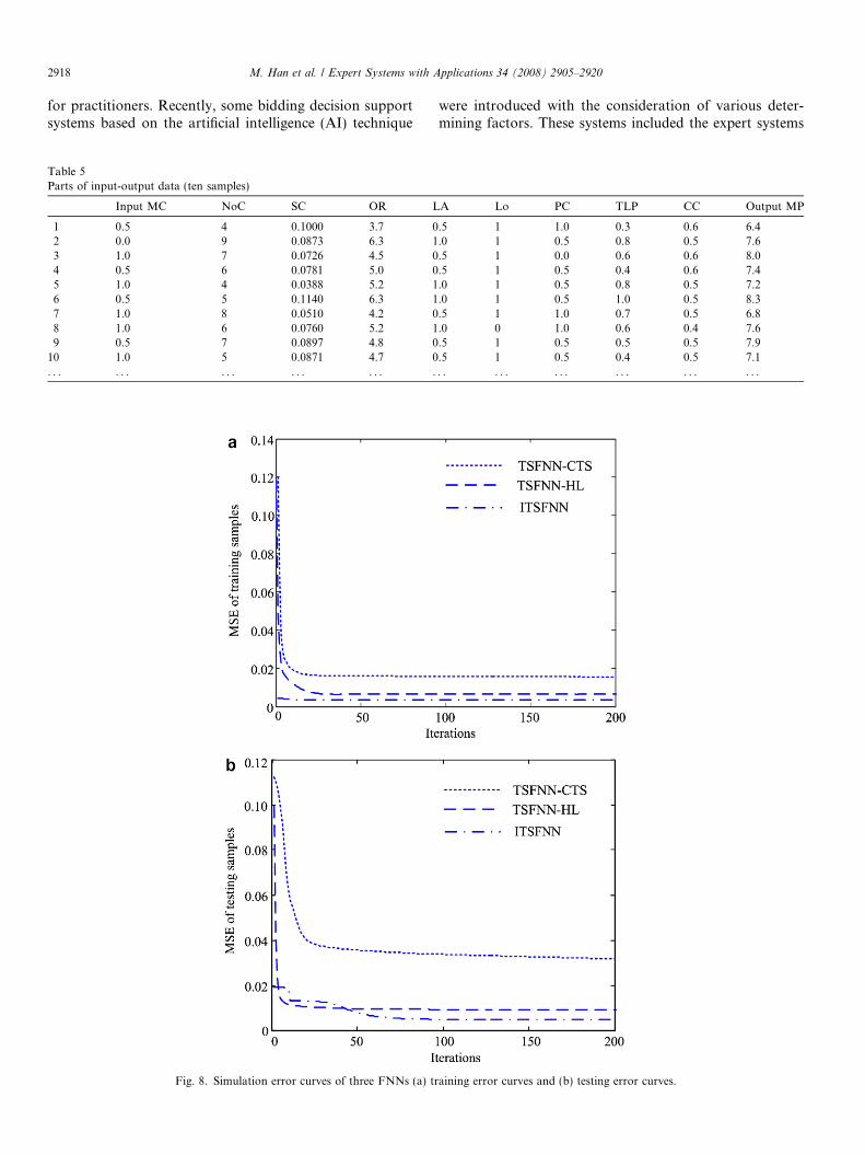
Fig. 8. Simulation error curves of three FNNs (a) tr

were introduced with the consideration of various deter-mining factors. These systems included the expert systems

A Lo PC TLP CC Output MP

.5 1 1.0 0.3 0.6 6.4

.0 1 0.5 0.8 0.5 7.6

.5 1 0.0 0.6 0.6 8.0

.5 1 0.5 0.4 0.6 7.4

.0 1 0.5 0.8 0.5 7.2

.0 1 0.5 1.0 0.5 8.3

.5 1 1.0 0.7 0.5 6.8

.0 0 1.0 0.6 0.4 7.6

.5 1 0.5 0.5 0.5 7.9

.5 1 0.5 0.4 0.5 7.1

. . . . . . . . . . . . . . . . .

aining error curves and (b) testing error curves.

Table 6Results comparison of three FNNs

Types of FNN Final training error (MSE) Final testing error (MSE)

FNN-CTS 0.0154 0.0317TSFNN-HL 0.0067 0.0092ITSFNN 0.0036 0.0046


developed by Dawood (1996), and neural network systemdeveloped by Hegazy and Moselhi (1994), Wanous, Bouss-abaine, and Lewis (2003), Li et al. (1999), and case-basedreasoning system developed by Chua et al. (2001). Consid-ering that the bid decision is dynamically changing andhighly unstructured, and is characterized by a significantdegree of uncertainty and subjectivity, it is too difficultfor any single artificial intelligence method to realize thecomplicated field problems effectively. So the combinationof two or more AI techniques becomes a popular researchfocus.

A series of recent advances in computational analysis(matrix calculations, expert systems, artificial neural net-works and fuzzy logic) has allowed the introduction of evenmore quantitative and qualitative factors in the develop-ment of bidding models in an attempt to capture the under-lying patterns in human behavior and intuition andincorporate them in bidding strategies. A neural networksystem learns from cases. However, its reasoning processis concealed from the decision maker, operating like ablack-box. The decision maker cannot trace the reasoningprocess. For this reason, conclusions derived from the neu-ral network are not very convincing to the decision maker.On the other hand, the reasoning process of fuzzy logic sys-tem can be more discernible to the decision maker. He canalso interact with and review the reasoning process andeven perform heuristic adjustments on the derived resultwhere necessary. Fuzzy logic system and neural networkshare the ability to improve the intelligence of systemsworking in uncertain, imprecise, and noisy environments.A promising approach is to combine them into an inte-grated system called fuzzy neural network, which possessesthe advantages of both NN and fuzzy system. More trans-parency is pursued by interpretation of the weight matrixfollowing the learning stage, and allowing automatic tun-ing of the parameters decrease the subjectivity of the fuzzysystem. Because the improved fuzzy neural network basedon T–S model has advantages of fuzzy logic system andneural network, it can be used to the bidding system in con-struction industry to estimate the markup percentage.

Identification of major factors that affect markup deci-sions has become a significant research area. Differentresearchers have identified and proposed different sets offactors (Li et al., 1999; Wanous et al., 2003). This paperuses nine factors as inputs of the network and the markuppercent (MP) is viewed as the output (Han, Fan, & Guo,2005). Table 4 shows the definitions and value ranges ofeach of the nine factors in the simulation. There are 75 bid-ding examples of building projects collected as the trainingand testing data from real engineering, which 70 examplesare chosen as training samples (parts of samples are shownin Table 5) and others are testing samples.

In the paper (Han et al., 2005) authors add a hiddenlayer to the consequent network contrasted to the ordinaryT–S model fuzzy neural network, called TSFNN-HL inthis paper, which is used to simulate the same data to pre-dict the bid markup. The fuzzy network proposed by Fior-

daliso (2001), denoted by TSFNN-CTS, is used to simulatethe data, too. Fig. 8 is the contrast of the simulation resultswith four models, including training errors and testingerrors, respectively. It is obvious that the ITSFNN pro-posed in this paper is given better performance, such ashigher precision, lower error and better generalization.Because the condition of bidding system is not entire sameto the past condition each time, testing data for estimatingthe markup may be different from training data. So thegeneralization of the neural network is more important inreality, and it determines the precision of estimation. It isobserved that the ITSFNN model has better generalizationability from Fig. 8b. Table 6 gives the final results on the200th iteration with different networks. Whatever simula-tion precision or prediction precision, ITSFNN is higherthan the other two networks. Consequently, the model pro-posed in the paper is much more appropriate in practice.

6. Conclusions

The paper proposed an improved fuzzy neural networkbased on T–S model. First according to characteristics ofsamples spatial distribution, fuzzy space is automaticallypartitioned reasonably, i.e. automatically and accuratelyconstructing membership functions. Then fuzzificationlayer and inference layer are connected by antecedent partsof rules. It simplifies the network structure. The process ofobtaining rules includes two steps. First the cluster centersare got by subtractive cluster method. Second the centersare fuzzified and the similar rules are merged to obtainthe importance of each rule. The antecedent and conse-quent parameters of ordinary T–S fuzzy neural networkare determined by experience or randomly. The paper,according to the properties of samples and the networkstructure, parameters are initialized to induce lower initialerror. The results of simulations verify this method. Twoexamples are used to verify the ITSFNN. Then it is appliedto construction bidding markup and compared with otherthree networks. The results show that the ITSFNN hasgood simulation precision and high generalization abilityin construction bidding markup prediction.

Acknowledgement

The work is supported by the National Natural ScienceFoundation of China under Project 60674073 and Project60374064. Both supports are appreciated.


References

Bortolan, G., & Pedrycz, W. (2002). Linguistic neurocomputing: thedesign of neural networks in the framework of fuzzy sets. Fuzzy Sets

and Systems, 128, 389–412.Carr, R. I. (1982). General bidding model. Journal of the Construction

Division, 108(4), 639–650.Chiu, S. (1994). Fuzzy model identification based on cluster estimation.

Journal of Intelligent & Fuzzy Systems, 2(3), 267–278.Christodoulou, S., & ASCE, A. M. (2004). Optimum bid markup

calculation using neurofuzzy systems and multidimensional riskanalysis algorithm. Journal of Computing in Civil Engineering, 18(4),322–330.

Chua, D. K. H., Li, D. Z., & Chan, W. T. (2001). Case-based reasoningapproach in bid decision making. Journal of Construction Engineering

and Management, 127(1), 35–45.Dawood, N. N. (1996). A strategy of knowledge elicitation for developing

an integrated bidding/production management expert system for theprecast industry. Advances in Engineering Software, 25(2), 225–234.

Fiordaliso, A. (2001). A constrained Takagi–Sugeno fuzzy system thatallows for better interpretation and analysis. Fuzzy Sets and Systems,

118(3), 307–318.Friedman, L. (1956). A competitive bidding strategy. Operations Research,

4(1), 104–112.Gates, M. (1967). Bidding strategies and probabilities. Journal of the

Construction Division, 93(1), 75–107.Gates, M. (1983). A bidding strategy based on ESPE. Cost Engineering,

25, 27–35.Han, M., Fan, Y., & Guo, W. (2005). A modified neural network based on

subtractive clustering for bidding system, IEEE international confer-

ence on neural networks and brain (pp. 128–133). Beijing, China.Hegazy, T., & Moselhi, O. (1994). Analogy-based solution to markup

estimation problem. Journal of Computing in Civil Engineering, 8(1),72–87.

Ishibuchi, H., & Nii, M. (2001). Numerical analysis of the learning offuzzified neural networks from fuzzy if-then rules. Fuzzy Sets and

Systems, 120, 281–307.Li, Z., Kevman, V., & Ichikawa, A. (2002). Fuzzified neural network

based on fuzzy number operations. Fuzzy Sets and Systems, 130,291–304.

Lin, C. J., & Xu, Y. J. (2006). A self-adaptive neural fuzzy network withgroup-based symbiotic evolution and its prediction applications. Fuzzy

Sets and Systems, 157, 1036–1056.

Lin, C. T., Yeh, C. M., Liang, S. F., Chung, J. F., & Kumar, N. (2006).Support–vector-based fuzzy neural network for pattern classification.IEEE Transactions on Fuzzy Systems, 14(1), 31–41.

Li, H., Shen, L. Y., & Love, P. E. D. (1999). ANN-based mark-upestimation system with self-explanatory capacities. Journal of Con-

struction Engineering and Management, 125(3), 185–189.Oh, S. K., Pedrycz, W., & Park, H. S. (2003). Hybrid identification in

fuzzy neural networks. Fuzzy Sets and Systems, 138, 399–426.Oh, S. K., Pedrycz, W., & Park, H. S. (2005). Multi-layer hybrid fuzzy

polynomial neural networks: a design in the framework of computa-tional intelligence. Neurocomputing, 64, 397–431.

Oh, S. K., Pedrycz, W., & Park, H. S. (2006). Genetically optimized fuzzypolynomial neural networks. IEEE Transactions on Fuzzy Systems,

14(1), 125–144.Ouyang, C. S., Lee, W. J., & Lee, S. J. (2005). A TSK-type neurofuzzy

network approach to system modeling problems. IEEE Transactions

on SMC–C, 35(4), 751–767.Papadakis, S. E., & Theocharis, J. B. (2002). A GA-based fuzzy modeling

approach for generating TSK models. Fuzzy Sets and Systems, 131,121–152.

Plamen, P. A., & Dimitar, P. F. (2004). An approach to onlineidentification of Takagi–Sugeno fuzzy models. IEEE Transaction on

SMC–B, 34(1), 484–498.Tang, A. M., Quek, C., & Ng, G. S. (2005). GA-TSKfnn: parameters

tuning of fuzzy neural network using genetic algorithms. Expert

Systems with Applications, 29, 769–781.Tao, C. W. (2002). Unsupervised fuzzy clustering with multi-center

clusters. Fuzzy Sets and Systems, 128, 305–322.Tung, W. L., & Quek, C. (2002). GenSoFNN: a generic self-organizing

fuzzy neural network. IEEE Transactions on Neural Networks, 13(5),1075–1086.

Wanous, M., Boussabaine, H., & Lewis, J. (2003). A neural network bid/no bid model: the case for contractors in Syria. Construction

Management and Economics, 21(7), 737–744.Wu, S., & Er, M. (2000). Dynamic fuzzy neural networks—a novel

approach to function approximation. IEEE Transactions on SMC–B,

30(2), 358–364.Yager, R., & Filev, D. (1994). Generation of fuzzy rules by mountain

clustering. Journal of Intelligent & Fuzzy Systems, 2(3), 209–219.Yu, W., & Li, X. (2004). Fuzzy identification using fuzzy neural networks

with stable learning algorithms. IEEE Transactions on Fuzzy Systems,

12(3), 411–420.

an improved fuzzy neural network based on t–s model

Documents