an improved evaluation method for airplane simulator motion cueing
TRANSCRIPT

AN IMPROVED EVALUATION METHOD
FOR AIRPLANE SIMULATOR MOTION CUEING
by
Alex Marodi
B.S. in E.E., University of Pittsburgh, 1991
Submitted to the Graduate Faculty of
the School of Engineering in partial fulfillment
of the requirements for the degree of
Master of Science
University of Pittsburgh
2002

UNIVERSITY OF PITTSBURGH
SCHOOL OF ENGINEERING
This thesis was presented
by
Alex Marodi
It was defended on
April 17, 2002
and approved by
M. A. Simaan, Ph. D., Professor, Electrical Engineering Thesis Advisor
ii

AN IMPROVED EVALUATION METHOD
FOR AIRPLANE SIMULATOR MOTION CUEING
Alex Marodi, M.S.
University of Pittsburgh, 2002
The lack of sufficient evaluation criteria for motion systems has contributed to
perceivable differences in motion cues among similar airplane simulators. To resolve
this issue, criteria for simulator motion cueing and evaluation must be developed to
insure uniform and optimum cues within a motion system’s workspace. Therefore, an
improved evaluation method is proposed to enable a better assessment of motion
cueing within the workspace.
To demonstrate the effectiveness of the improvement, an off-line simulation of a
motion system is developed and used for the evaluation. A common motion cueing
algorithm is incorporated in the simulation to control a motion platform model. Test
signals that approximate typical airplane specific forces, for selected maneuvers, are
used to drive the simulation. During each simulation test run, a platform trajectory is
recorded for the maneuver. The trajectory data are then processed by an optimization
routine that determines the dynamic workspace limits as a function of the trajectory. The
time histories of the trajectory and the workspace limits are then plotted for evaluation.
Presenting the platform trajectory along with the dynamic workspace limits
provides another way of evaluating the quality of motion cues within the workspace.
iii

Augmenting the existing motion criteria that are used in current evaluation methods with
criteria based on the dynamic workspace limits yields an improved evaluation method.
This improved evaluation method contributes to the development of criteria for motion
evaluation.
iv

ACKNOWLEDGEMENTS
I would like to thank Dr. M. A. Simaan, my advisor, for his guidance and
assistance in the preparation of this thesis.
Also, I would like to thank Prof. F. Cardullo and Mr. R. Telban of the State
University of New York at Binghamton for providing information on their contributions to
the on-going research in the field of motion cueing.
I would especially like to thank my wife, Annette, and children, Luke, Rachel,
Anna, and Leah, for their patience, understanding, and support.
v

TABLE OF CONTENTS
1.0 INTRODUCTION....................................................................................................... 1
1.1 Motivation ............................................................................................................ 1
1.2 Research Objective.............................................................................................. 3
1.3 Outline ................................................................................................................. 6
2.0 DESCRIPTION AND MATH MODEL OF A MOTION SYSTEM ................................. 8
2.1 Introduction .......................................................................................................... 8
2.1.1 Airplane Simulator Motion System............................................................... 8
2.1.2 Basis for the Motion System Regulatory Requirement .............................. 11
2.1.3 Psychophysical Perception of Motion ........................................................ 12
2.1.4 Concept of Motion Cueing ......................................................................... 15
2.2 Math Model of a Motion System......................................................................... 17
2.2.1 Motion System Input Component .............................................................. 19
2.2.1.1 Radius Vector R and the Motion System Reference Point ................ 24
2.2.2 Motion Cueing Component ........................................................................ 27
2.2.2.1 Scaling and Limiting .......................................................................... 29
2.2.2.2 Frame Transformations ..................................................................... 31
2.2.2.3 Adaptive Filtering............................................................................... 35
2.2.2.4 Integration ......................................................................................... 47
2.2.3 Motion Actuator Transformation Component ............................................. 49
2.2.4 Motion Actuator Model Component ........................................................... 54
vi

2.3 Summary ........................................................................................................... 54
3.0 EVALUATION OF MOTION CUEING...................................................................... 56
3.1 Introduction ........................................................................................................ 56
3.2 Current Motion Qualification Criteria and Evaluation Issues .............................. 56
3.2.1 Current Motion Qualification Criteria.......................................................... 56
3.2.2 Motion Evaluation Issues........................................................................... 58
3.3 Motion Workspace Evaluation............................................................................ 60
3.3.1 Motion Actuator Inverse Transformation .................................................... 62
3.3.2 Optimization Routine to Solve the Dynamic Workspace Limits.................. 67
3.3.3 Simulation Results and Discussion............................................................ 73
3.4 Improved Method for Evaluating Motion Cueing ................................................ 81
3.4.1 Combining Inverse Transformation and the Workspace Limits Routine..... 83
3.4.2 Simulation Results and Discussion............................................................ 85
4.0 DISCUSSION AND CONCLUSION......................................................................... 97
4.1 Discussion ......................................................................................................... 97
4.2 Conclusion ......................................................................................................... 98
BIBLIOGRAPHY ......................................................................................................... 100
vii

LIST OF TABLES
Table 2.1 Values for the Adaptive Filter Parameters ............................................... 49
Table 2.2 Coordinates for the Actuator Attachment Points ...................................... 52
Table 3.1 Typical Motion Performance Limits.......................................................... 61
viii

LIST OF FIGURES
Figure 2.1 Airplane Simulator with a Six Degrees-Of-Freedom Motion System........ 9
Figure 2.2 Factors that Influence Pilot-Airplane Performance................................. 12
Figure 2.3 Basic Structure of Motion and Orientation Perception Model................. 13
Figure 2.4 Perception Model Response to Visual and Inertial Motion Cues ........... 15
Figure 2.5 Block Diagram of Typical Motion System............................................... 18
Figure 2.6 Definition of Vector Components in the Airplane Equations of Motion ... 20
Figure 2.7 Centroid of the Motion System Platform ................................................ 25
Figure 2.8 Illustration of Airplane, Simulator, and Inertial Reference Frames ......... 26
Figure 2.9 Block Diagram of the Motion Cueing Component .................................. 28
Figure 2.10 Scaling and Limiting Function for fx,c,o .................................................. 30
Figure 2.11 Motion System Geometry..................................................................... 50
Figure 2.12 Vector Diagram for Actuator i ............................................................... 51
Figure 3.1 Steepest Descent Flow Chart for Dynamic Workspace Limits ............... 71
Figure 3.2 Z Axis Upper Limit Search Trajectory..................................................... 73
Figure 3.3 Z Axis Lower Limit Search Trajectory..................................................... 74
Figure 3.4 Z Axis Upper Limit Search Trajectory..................................................... 75
Figure 3.5 Z Axis Lower Limit Search Trajectory..................................................... 76
Figure 3.6 Motion Workspace Limits for αn = [0,0,0,0,0,0] ...................................... 77
Figure 3.7 Motion Workspace Limits for αn = [1,0,0,0,0,0] ...................................... 79
ix

Figure 3.8 Motion Workspace Limits for αn = [0.5,0,0,0,0.2,0] ................................ 80
Figure 3.9 Flowchart for the Off-line Motion Simulation .......................................... 82
Figure 3.10 Simplified Motion Block Diagram ......................................................... 84
Figure 3.11 Motion Block Diagram with Motion Data Post Processing System....... 85
Figure 3.12 Test Case 1: Specific Force Inputs and Platform X Acceleration.......... 88
Figure 3.13 Test Case 1: Platform Positions and Workspace Limits ....................... 89
Figure 3.14 Unfiltered and Filtered Zplatform Limit Signals......................................... 91
Figure 3.15 Filtered Zplatform Limit Signals................................................................ 92
Figure 3.16 Test Case 1A: Specific Force Inputs and Platform X Acceleration ....... 93
Figure 3.17 Test Case 1A: Platform Positions and Workspace Limits..................... 94
Figure 3.18 Test Case 1B: Platform Positions and Workspace Limits..................... 96
x

1.0 INTRODUCTION
1.1 Motivation
Airplane simulator qualification criteria are used to determine if a simulator
complies with federal regulations.(1)* Federal regulations require motion systems on all
airplane simulators that are qualified for use in approved pilot training programs. Thus,
motion criteria are a part of the simulator qualification criteria.
The current motion evaluation criteria, which are over twenty years old, do not
validate the integration of the motion system with the flight dynamics. The criteria are
primarily used to validate stand-alone hardware characteristics, like frequency response
and smoothness of movement. Apparently, due to the lenient criteria, motion systems
that provided questionable simulated motion cues1 have been qualified. For this reason,
it is contended that the current criteria are insufficient for evaluating motion performance
and must be developed.(2-5)
Since the late 1980s, several attempts have been made by the aviation industry
to develop the motion criteria.(2,3) Industry working groups composed of representatives
of the airlines, authorities, and simulator manufacturers have convened to review all of
_______________ *Parenthetical references placed superior to the line of text refer to the bibliography. 1Cue is defined here as a stimulus that elicits a percept.
1

the systems covered by the airplane simulator qualification criteria, including motion.
Generally, most modification proposals have been incorporated, but motion proposals
have been tabled due to opposition by a significant segment of the industry. The
reasons for this are not clear, but could be attributed to several things. For instance,
motion cueing is probably one of the least understood branches of simulation, and
objective criteria are not readily apparent. Also, the effects of motion cues on pilot
performance are not fully understood. In addition, a segment of the industry feels that
motion is not needed on simulators with improved visual display systems. So, the
evaluation of motion cueing remains largely a subjective assessment.
In the latest attempt by industry to develop the criteria, the motion proposals(48)
still do not address some evaluation issues.(5,47) Criteria are proposed to insure that the
motion system performs as originally qualified. But, criteria that insure uniform and
optimum cues within a motion system’s workspace* are not addressed in detail.
So, although there is consensus that the current criteria are inadequate,
consensus on what constitutes sufficient criteria has not been reached. The
development of methods for motion evaluation, however, should not be impeded until
appropriate criteria can be fully determined. It has been said that, “Any method of
attaching degrees of objectivity to the quality of the motion system should therefore be a
better assessment than just checking [hardware] performance in isolation….”(4)
_______________ *The workspace is the maximum usable translational and rotational mechanical travel of the motion platform.
2

1.2 Research Objective
Motion cueing contributes to perceptual fidelity by attempting to provide the
flight crew with optimum motion (force) cues within the workspace of the motion system
that are representative of the airplane cues. One area(26) of active research is human
centered motion cueing which incorporates models of the human vestibular sensation
system within the cueing algorithm in an attempt to achieve the best perceptual fidelity.
But, as important as motion cueing is to perceptual fidelity, it is still only evaluated
subjectively. As a result, there are concerns that motion systems are not being driven to
induce the best perceptual, and therefore behavioral, fidelity. On-going research(40-43) is
being conducted to formulate appropriate motion fidelity criteria to more objectively
evaluate motion cueing. Because of the complexities of human factors, proper criteria
have been difficult to define. Other criteria(48) that have been recently proposed by
industry focus primarily on cue repeatability. Validating that cues are repeatable,
however, does not mean the cues are appropriate.
A couple of outstanding cueing issues that apparently have not received a lot of
discussion involve the operating envelope, or workspace, of the motion system. The
workspace determines the cueing ability of the motion system. The workspace is
therefore an important factor in motion fidelity. Most airplane simulators utilize multiple-
degrees-of-freedom motion systems (e.g., surge, pitch, roll, and heave motion) whose
identical actuators are constrained by their minimum and maximum lengths and thus
impose a workspace that the moving platform can achieve with respect to its inertial
frame. This means that the motion system excursions in certain degrees-of-freedom
restrict excursions in the others. Consequently, motion cues are limited in the restricted
3

degrees of freedom. The outstanding issues then are how much of the workspace is
being used during normal operation and what amount of workspace is required to
provide effective motion cues. The latter concern involves human factors and is difficult
to define. So, the aim of this thesis addresses how much of, and how well, the
workspace is being used. Of course, a motion workspace cannot be readily described
because of the infinite number of possible combinations of excursions. In this case, a
means of qualitatively judging how the workspace is being used, or the amount it is
being restricted, by the motion cueing system would be a useful improvement.
Firstly, to gain a better understanding of the problem and potential criteria,
several disciplines involved in the development of motion systems were first
investigated. Literature on both the background and techniques of motion cueing were
examined.(6-27) As it turned out, an adaptive cueing technique is the most commonly
used in industry, so it is used for this research. The proper transformations of the
simulated airplane’s inertial signals, that are processed by the cueing algorithm, were
reviewed in the flight dynamics literature.(28-30) Since human factors is an integral part of
motion cueing design, both the design of experiments for pilot evaluations of simulator
motion(31-35) and the physiological and psychophysical aspects of motion perception(37-43)
were studied. Also, the mechanical design and performance of typical motion systems
were reviewed.(44-46) After investigating each discipline, optimization techniques(49-50)
were examined with the intent of using them to develop a better method of evaluating
motion cueing within the workspace limits.
Secondly, since it was decided that it is desirable to observe and analyze the
changing workspace limits temporally for a recorded actual platform trajectory, this
4

motivates the development of an optimization method that determines the dynamic
workspace limits as a function of the actual platform trajectory. The optimization
technique employed here to solve the workspace limits is of the type used to solve
unconstrained optimization problems. The technique is based on a steepest descent
method using a constant step size. To determine the dynamic workspace limits for a
given platform trajectory, the steepest descent method is used in a stepwise manner to
search for the limits in each degree of freedom (surge, sway, heave, pitch, roll, and
yaw), throughout the trajectory. The algorithm steps through each platform position
sample in the trajectory data. At each sample, the algorithm sequences through each of
the six degrees-of-freedom position points within the sample, starting with surge, while
fixing the other five degrees-of-freedom points to their values at that time. The specified
maximum workspace limits for the current degree-of-freedom being searched are
selected for use in the steepest descent’s quadratic objective function. The objective
function is simply the squared difference of the value of the current degree-of-freedom
position point and the value of the current degree-of-freedom’s excursion limit. The
gradient of the objective function and the constant step size are used to iterate the
steepest descent algorithm towards the actual upper and lower workspace limits in each
degree-of freedom by updating the current degree-of-freedom position point until the
stopping criterion is met in both directions. This is done for every platform position
sample in the trajectory.
Thirdly, in order to use this new workspace limits routine, an actual platform
trajectory must be recorded on the simulator. A device that is used to do this is the
motion actuator inverse transformation that was contributed in a previous study.(9) It
5

enables the computation of the actual platform position based on the magnitude of the
actuator extensions. The actuator inverse transformation is combined with the dynamic
workspace limits routine to compute the workspace limits from the platform trajectory.
Finally, the effectiveness of this improvement is demonstrated using an off-line
simulation of a motion system that is developed for the evaluation. An adaptive motion
cueing algorithm is incorporated in the simulation to control a model of a motion
platform. Test signals that approximate typical airplane specific forces are used to drive
the simulation. During each simulation test run, a platform trajectory is recorded for the
maneuver. The trajectory data are then processed by the optimization routine that
determines the dynamic workspace limits as a function of the trajectory. The time
histories of the trajectory and the workspace limits are then plotted for evaluation.
Thus, this thesis presents a viable approach to evaluating the use of the motion
workspace. This improvement gives the evaluator another means of assessing if the
workspace is being used optimally. Presenting the platform trajectory along with the
dynamic workspace limits provides an effective way of evaluating the quality of motion
cues within the workspace. And, the method can be used to detect possible real-time
hardware or software anomalies. Augmenting the existing motion criteria that are used
in current evaluation methods with criteria based on the dynamic workspace limits yields
an improved evaluation method.
1.3 Outline
This thesis comprises 4 chapters. The first chapter introduces the motivation and
research objective for the development of an improved evaluation method for motion
6

cueing. Chapter 2 describes a typical motion system and a motion system model that is
used for this research. The improved evaluation method is presented and demonstrated
in Chapter 3. Chapter 4 discusses the results and recommends further work on the
evaluation of motion cueing performance.
A few comments must be made on the background material provided in Chapters
2 and 3. The intent of the background material on an airplane simulator’s motion system
and motion math model is to provide insight into the nature of motion cueing and to
enable a better understanding of motion cueing evaluation issues. Described in the
background material are certain devices, like the motion cueing algorithms and actuator
transformations, that were contributed by past studies and are used to develop the
workspace limits routine in this study. The author claims no credit for the development of
this background material and is presenting it, along with the pertinent references, to
establish the framework within which the author’s contribution is developed and
demonstrated.
Although this extensive preparatory material could be considered excessive for
this study, the author feels that it is useful to include this material so that the study is
cohesive and self-contained. That is, the goal is to provide a sufficient amount of
background information so that the reader does not have to acquire the referenced
studies in order to understand the contribution of this study. Hopefully, the reader who is
unfamiliar with motion systems and the evaluation issues will appreciate this format. On
the other hand, readers who are familiar with the subject matter can cursorily review
Chapter 2 and the beginning of Chapter 3.
7

2.0 DESCRIPTION AND MATH MODEL OF A MOTION SYSTEM
2.1 Introduction
This chapter introduces the basic principles of an airplane simulator’s motion
system and presents a mathematical model of a typical system. The intent is to enable a
better understanding of motion cueing evaluation.
The description of the motion system includes the motion system configuration,
the basis for the regulatory requirements, the psychophysical perception of motion, and
the concept of motion cueing. This review provides insight into the nature of motion
cueing.
The math model that is presented is the basis of the off-line simulation that is
used, in the next chapter, to develop an improved evaluation method for motion cueing.
It is composed of motion input, adaptive cueing, actuator model and actuator
transformation components.
2.1.1 Airplane Simulator Motion System
An airplane simulator is a full size replica of a specific airplane cockpit, and it is
capable of representing the airplane in ground and flight operations. It is equipped with
visual, sound, flight control, and motion sub-systems. All required cockpit components
and sub-systems are interfaced to high-speed digital computers. These computers host
real-time simulation software that simulates the airplane and its environment.
8

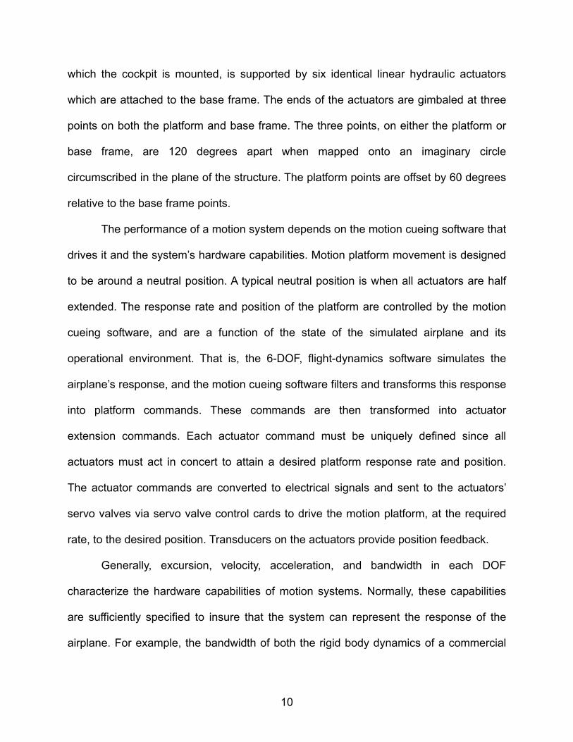
Of all the sub-systems, the conventional motion system is perhaps the least
capable of fulfilling its purpose. That is, it cannot simulate sustained accelerations
because its workspace is physically limited. This limitation is obvious in Figure 2.1 that
depicts an airplane simulator equipped with a six degrees-of-freedom (DOF) motion
system, in a neutral position and pitched up. Although commercial three and four DOF
systems exist, only a six DOF configuration is considered in this research since it is the
most common and complex. Six DOF systems are required on FAA Level C and D
simulators.(1)
a) neutral position b) pitched up
Figure 2.1 Airplane Simulator with a Six Degrees-Of-Freedom Motion System
The design of a conventional six DOF motion system is based on the Stewart
platform.(44) The hardware consists of a motion platform, capable of limited rotational
(pitch, roll, and yaw) and translational (surge, sway, and heave) movement, a motion-
drive electronics interface cabinet, and a hydraulic power unit.(6) The platform, upon
9
which the cockpit is mounted, is supported by six identical linear hydraulic actuators
which are attached to the base frame. The ends of the actuators are gimbaled at three
points on both the platform and base frame. The three points, on either the platform or
base frame, are 120 degrees apart when mapped onto an imaginary circle
circumscribed in the plane of the structure. The platform points are offset by 60 degrees
relative to the base frame points.
The performance of a motion system depends on the motion cueing software that
drives it and the system’s hardware capabilities. Motion platform movement is designed
to be around a neutral position. A typical neutral position is when all actuators are half
extended. The response rate and position of the platform are controlled by the motion
cueing software, and are a function of the state of the simulated airplane and its
operational environment. That is, the 6-DOF, flight-dynamics software simulates the
airplane’s response, and the motion cueing software filters and transforms this response
into platform commands. These commands are then transformed into actuator
extension commands. Each actuator command must be uniquely defined since all
actuators must act in concert to attain a desired platform response rate and position.
The actuator commands are converted to electrical signals and sent to the actuators’
servo valves via servo valve control cards to drive the motion platform, at the required
rate, to the desired position. Transducers on the actuators provide position feedback.
Generally, excursion, velocity, acceleration, and bandwidth in each DOF
characterize the hardware capabilities of motion systems. Normally, these capabilities
are sufficiently specified to insure that the system can represent the response of the
airplane. For example, the bandwidth of both the rigid body dynamics of a commercial
10
airplane and pilot control is typically limited to 2.0 Hz, or less.(6) So, the magnitude of the
motion system’s frequency response is usually near unity up to this frequency with
minimal phase lag so that flying qualities are adequately reproduced.(1,45)
2.1.2 Basis for the Motion System Regulatory Requirement
Currently, a motion system is required on an airplane simulator to comply with the
regulatory requirement for a system that provides motion (force) cues that are perceived
by the pilot to be representative of the airplane motions.(1) The general requirement for
motion was first added to the FAR in the 1960s based on the perceptual theory that
critical sensory elements must be included to achieve sufficient perceptual and
behavioral fidelity.(2,38,39)
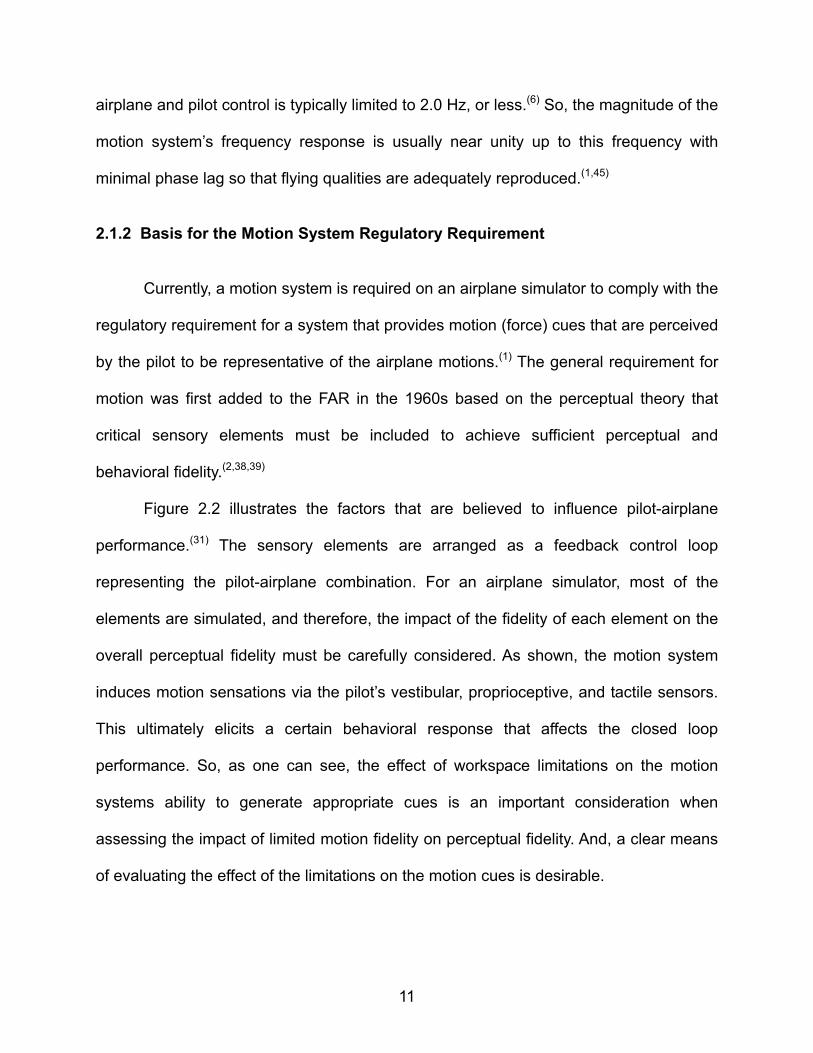
Figure 2.2 illustrates the factors that are believed to influence pilot-airplane
performance.(31) The sensory elements are arranged as a feedback control loop
representing the pilot-airplane combination. For an airplane simulator, most of the
elements are simulated, and therefore, the impact of the fidelity of each element on the
overall perceptual fidelity must be carefully considered. As shown, the motion system
induces motion sensations via the pilot’s vestibular, proprioceptive, and tactile sensors.
This ultimately elicits a certain behavioral response that affects the closed loop
performance. So, as one can see, the effect of workspace limitations on the motion
systems ability to generate appropriate cues is an important consideration when
assessing the impact of limited motion fidelity on perceptual fidelity. And, a clear means
of evaluating the effect of the limitations on the motion cues is desirable.
11
Tasks•Control •Auxiliary
Task PilotCockpitInterface
Stabilityand Control
CharacteristicsAirplane
EnvironmentTask
Performance
Pilot
Stress•Distraction
•Surprise fromdisturbance
Visual Info•External•Instruments
Vestibular / Tactile/ Proprioceptive
Info•Motion Cues•Disturbances
PrimaryControls
Selectors
Aircraft State(Normal or Failure)•Configuration•Weight•Mass Distribution
TaskPerformance
Stabilityand Control
Characteristics
AirplaneMotion
EnvironmentalState
•Day/Night•Weather•Visibility
Figure 2.2 Factors that Influence Pilot-Airplane Performance
(Adapted from Reference 31)
In the 1960s, preliminary studies showed that pilot performance improved when
certain maneuvers were accompanied by appropriate motion cues. As a result, the FAA
adopted the conservative position that motion is critical, even though, to this point, there
is no conclusive evidence that transfer of behavior, from simulator to airplane, is
affected.(6,35) The requirement is also backed by pilots’ feelings that motion improves
realism and is helpful for maneuvering.(32,33)
2.1.3 Psychophysical Perception of Motion
The mere provision of motion does not guarantee perceptual fidelity or that the
simulator will be more effective. The motion cues must be properly integrated and
synchronized with the other critical sensory elements shown in Figure 2.2, like the visual
element.(37-43) Otherwise, perceptual conflicts can occur and result in a deleterious
12

behavioral response. Due to the motion workspace limitations, the nature of motion
perception must be understood to effectively integrate and synchronize the motion cues.
Figure 2.3 depicts one model of human motion perception that can be used for
discussion.(6)
PsychophysicalCentral
Processor
EstimationProcessUsing
SensoryInput
Impulses
PerceptualState
EstimateOf Motion
AndOrientation
Physiological Sensory Models
Visual
Vestibular
Proprioceptive
Tactile
Stimuli
•Motion•Visual•Haptic•Proprioceptive
Figure 2.3 Basic Structure of Motion and Orientation Perception Model
(Adapted from Reference 6)
The model consists of a physiological stage containing the sensors that convert
physical energy into afferent neural impulses, and a psychophysical stage that
organizes the stimuli into meaningful patterns. The vestibular system, the non-auditory
portion of the inner ear, is primarily a sensitive sensor of linear and rotational
accelerations. Static body tilt is sensed by the proprioceptors as a change in the
direction of the specific force vector (acceleration less gravity), which is virtually
indistinguishable from a change caused by linear acceleration. Note then, that a
sensation of sustained acceleration can be induced to some extent if the motion
platform is properly tilted. The tactile sensors detect force applied to the external surface
13

of the body. The psychophysical estimation forms a perception of motion as a function
of the neural impulses, state of mind, the environment, and experience.
The frequency responses and thresholds of the sensors affect motion perception
and also must be considered. The vestibular and other proprioceptive sensors are most
sensitive in the mid-range of the applicable frequency spectrum. The visual sensors are
most sensitive at the lower frequencies, while the tactile sensors are most sensitive at
the higher frequencies. Research(38-42) has shown that lengthy, detrimental time delays
in motion perception can occur when relying only on visual sensors during sudden
accelerations of a visual scene. The delays were alleviated, however, when the visual
cue was coordinated with a force cue induced by a slight motion platform displacement.
Studies(39) have also shown that force cues elicit lead compensation from the pilot to
stabilize the airplane during high-gain pilot-in-the-loop maneuvers, like tracking
maneuvers. Figure 2.4 illustrates the model’s response to an angular rate stimulus.
Note that the perception of motion is much improved when the visual and force cues are
properly integrated and synchronized.
The stimulation of the non-visual sensors will result in the earliest recognition of
motion and proper behavioral response, provided that the stimulus exceeds the sensors’
sensitivity thresholds. This is the importance of properly stimulating these sensors in
airplane simulators.
14

Time, sec
Stimulus
Perceived withvisual and inertialcues
Perceived withInertial cues only
Perceived withvisual cues only
AngularRate,deg/sec
20
40
1.5
3.0
Figure 2.4 Perception Model Response to Visual and Inertial Motion Cues (Adapted from Reference 6)
2.1.4 Concept of Motion Cueing
The concept of motion cueing is to track, in real time, the specific forces and
angular accelerations of the simulated airplane while limiting the simulator’s motion
platform within its workspace.(7,12,22,39) To meet these conflicting objectives, the inertial
signals must be modified to drive the motion platform in a manner to reproduce at least
a portion of the motion cues that the pilot would perceive in the airplane. At best, the
motion system can provide the pilot with a satisfactory perception of these cues. Motion
cues are coordinated with visual display and instrument cues to induce a proper
perception of motion. Cues that are uncharacteristic of the airplane must not be
generated.
Motion cueing is accomplished by a motion cueing algorithm. The algorithm
attempts to yield optimum and realistic motion cues in the process of modifying the
15

inertial signals. The modifications include various transformations and filtering of the
signals. Transformations are required to transform the signals from airplane to simulator
reference frames, and to convert platform commands to unique actuator commands.
High- and low-pass filters are used, along with attenuation and limiting, to keep the
platform within the workspace while generating appropriate cues.
A motion cue is basically composed of an onset cue and, if applicable, a
sustained cue. An onset cue simulates the initial acceleration of the airplane. This cue is
produced by passing the airplane acceleration through high-pass, or washout, filters to
remove the low-frequency component that would drive the platform to its limits. Thus,
this cue is maintained for only a short duration. For a linear surge or sway airplane
acceleration, if the low-frequency component persists as the onset cue subsides, a
sustained cue is blended with the onset cue to produce a sense of continuous
acceleration.
Cross-feeding the linear surge or sway acceleration through low-pass filters to
the corresponding rotational channel produces the sustained cue (a.k.a., tilt
coordination). The rotational channel tilts the platform to simulate sustained linear
acceleration via static body tilt (a.k.a., gravity vector alignment).(17,18) For example,
during forward (surge) acceleration, the onset surge cue is blended with a sustained
cue that is produced by pitching the platform. The platform is pitched up at a rate equal
to the washout rate of the onset cue. The pitch attitude is proportional to the sustained
linear acceleration of the airplane. The coordination between the onset and sustained
cues is such that effective motion cue perceived by the flight crew remains constant.
16

Incidentally, tilting the platform during the sustained cue does not affect any other
simulator cueing system, i.e., visual or instruments.
Attempts to provide cues beyond the capabilities of the platform are often more
confusing and adverse to the pilot than the complete absence of these cues. To ensure
that the motion system is capable of continuous movement, and ready to provide
subsequent cues, onset and sustained cues are “washed-out” at a rate below the flight
crew’s threshold of conscious perception. So, the platform imperceptibly returns to the
neutral or near-neutral position. The washout rates must be below the perceptual
thresholds; otherwise a washout cue could adversely affect pilot behavior.
2.2 Math Model of a Motion System
Figure 2.5 is a block diagram of a typical motion system. This diagram represents
the main components of the off-line simulation of the motion system that is developed
and used for the evaluation of motion cueing within the workspace.
The simulation is composed of input, motion cueing, actuator transformation, and
motion platform components. The input signals used to drive the off-line simulation
approximate typical airplane specific forces. The input component transforms the input
signals to the motion centroid, a reference point within the workspace. The motion
cueing component then filters the signals to provide both translational and rotational
motion platform position commands. Next, the position commands are converted into
actuator extension commands via the actuator transformation, and, finally, the extension
commands drive the six degrees-of-freedom motion platform component.
17

An adaptive cueing algorithm, a predominant motion cueing technique, is used
for the cueing component. As explained before, the motion system cannot provide
sustained cues because its workspace is physically limited. So, this algorithm attempts
to provide the best cues possible within the confines of the workspace by adjusting filter
parameters to minimize cost functions.
The math models of the components are given in the following sections. The
input component is covered first, followed by the motion cueing, actuator transformation,
and actuator model components.
ω
MOTION CUEING
TransformCG to
Centroid
Scale&
Limit
•Transform to Inertial Frame •Washout Filtering•Integration
•CrossfeedChannelTilt-Coordination•LP Filtering•Integration
•Transform to Inertial Frame•WashoutFiltering•Integration
+
X,Y,Z Translational
PositionCommands
(sway, surge, heave)
θ, φ, ψAngularPosition
Commands
fcg
ACTUATORTRANSFORMATION
ANGULAR DOFAngularacceleration:dω/dt= [P ,́Q́ ,R ]́t
Rotationalvelocity:ω=[P, Q, R]t
FLIGHT DYNAMICS
Body AxesEquations of Motionof the Airplane C.G.
TRANSLATIONALDOF
Specific force:
fcg =[fx, fy, fz]t
Real-Time Software Simulation Motion Hardware
+
SpecialEffects
+
Buffets/Runway
Roughness/Braking
Buffets/Runway
Roughness/Braking
Commands
TransformX,Y,Z,θ, φ, ψ
toLeg
ExtensionCommands
With Lead
Comp.(i = 1 - 6)
MOTION PLATFORM
Valve
ActuatorServoSystem
Sensor
Actuator i
(i = 1 - 6)Force and Pos.Feedback
Low-FreqComponent
High-FreqComponent
d ω/dt
INPUT
Scale&
Limit
Scale&
Limit
Figure 2.5 Block Diagram of Typical Motion System
18

2.2.1 Motion System Input Component
Previous motion cueing studies(7,17,18,20,37) affirm that a pilot senses the same
airplane translational accelerations and rotational rates that can be sensed by three
linear accelerometers and three rotational rate gyros installed at the pilot’s location.
Accelerometers sense linear motions along an axis while rate gyros sense angular
motion about an axis. Each set of devices is presumed to be orthogonally configured
and aligned with the airplane’s body-fixed XYZ coordinate system. The XYZ coordinate
system, or XYZ frame, is defined as a conventional right-handed coordinate system with
its origin at the airplane’s center of gravity (cg) as shown in Figure 2.6. It is designated
as Fb.
The idea then is that, if the simulator’s motion system is driven by, and responds
appropriately to, simulated accelerometer and rate gyro command signals, the pilot will
sense onset accelerations and rotational rates that are similar to the airplane’s.
Therefore, equations for accelerometers and rotational rate gyros are now developed
using inertial quantities from the airplane’s equations of motion. Since the inertial
quantities are computed at the cg, they must be transformed to the appropriate
coordinates to drive the motion system.
During translational motion, three accelerometers(28,29) sense inertial
accelerations and resolve them into the X, Y, and Z axes of the airplane, which is
assumed to be a rigid body. Each sensor provides an output signal proportional to the
difference between the acceleration of its case and gravitational acceleration. In the
literature, this difference is called the specific force. Expressing these three signals in
vector form, the specific force vector fcg is then given by
19

gafcg −= (2-1)
where a is the airplane’s inertial acceleration vector and g is the gravitational
acceleration vector. Rewriting this equation by expressing a in terms of the body and
gravitational forces defined in Figure 2.6, and resolving all quantities into the body axes,
yields
mB
mmB Bt
tB FggFfcg =−
+= (2-2)
where FB is the vector sum of the body-axis aerodynamic, FA, and thrust, FT, forces
acting at the cg. Bt is the transformation matrix that rotates g into the body axes at the
cg, and m is the mass of the airplane. Bt will be discussed later.
X
Y
ZAerodynam ic and Thrust Forces
FA y and FT y
FA z and FT z
FA x and FT x
Y
Acceleration of Gravity
ggz
gy
gxX
X
Y
Z
M A and M T N A and NT
LA and LT
Aerodynam ic and Thrust Moments
Linear and RotationalVelocities
(+ roll right)
(+ pitch up) (+ yaw right)
X
Y
Z
(+ roll right)
(+ pitch up)
(+ yaw right)
Z Zi inertial frame
wv
u
P
RQ
Figure 2.6 Definition of Vector Components in the Airplane Equations of Motion
(Adapted from Reference 29.)
20

Next, equation (2-2) must be modified so that the specific force can be computed
at coordinates other than the cg of the airplane. This is required because a typical
motion system is usually driven about a reference point that does not coincide with the
airplane’s cg. Generally, if the accelerometers are located at a point other than the cg,
rotational motion of the airplane affects these sensors in addition to the linear motion.
From classical mechanics(29,30), the inertial velocity of an alternate location c within the
airplane is given by
)( Rvv ×+= ωc (2-3)
where v is the airplane’s inertial velocity vector at the cg, ω is the inertial rotational
velocity vector of the airplane, and R is the radius vector from the cg to the alternate
location c. Differentiating equation (2-3) with respect to the inertial reference frame
(earth-fixed and indicated by subscript I) yields the inertial acceleration
IIIc dt
ddt
ddt
d )()()( RaRva ×+=
×+=
ωω (2-4)
For the accelerometer outputs, the terms must be expressed in the body frame.
From equation (2-2), notice that the first term, a, is equal to
m
mBtB gFa +
= (2-5)
The theorem of Coriolis(49), which defines the transformation of the time
derivative between two coordinate systems, is used to obtain the derivative of the
second term. Applying this theorem, the derivative of this cross product is
21
)()()( RRR××+
×=
×ωω
ωω
bI dtd
dtd (2-6)
In the airplane XYZ frame (indicated by subscript b), the derivative of the cross
product in the first term of equation (2-6) follows the product rule for differentiation:
)()()( RRR×+×=
×ωω
ω
bdtd
The dot indicates a quantity’s time derivative. Since R is constant in the XYZ
frame, the second term is zero, and equation (2-6) is rewritten as
)()()( RRR××+×=
×ωωω
ω
Idtd (2-7)
Substituting the expressions developed in equations (2-5) and (2-7) for the terms
in equation (2-4) yields
)()( RRgFa ××+×++
= ωωωm
mB tB
c (2-8)
Finally, by replacing a in equation (2-1) with ac in equation (2-8), the specific force
vector fc in the XYZ frame at location c is
gRRgF
f tt
Bc B
mmB
−
××+×+
+= )()( ωωω
Combining terms and using equation (2-2), the final form of fc is
22

)()( RRff cg ××+×+= ωωωc (2-9)
Note that the second term in equation (2-9) is the tangential acceleration part of
fc, and the third term is the centripetal acceleration. The three components of fc along
the X, Y, and Z axes are used as the translational inputs to the motion cueing
algorithms. Written in component form, equation (2-9) becomes
)()()(
)()()(
)()()(
22,,
22,,
22,,
QPRPQRRQRPRff
PRQRRPRRPQRff
QRPRRPQRRQRff
zyxzocz
zyxyocy
zyxxocx
+−++−+=
−++−++=
++−++−=
(2-10)
The rotational quantities P, Q, R, and their time derivatives that are used in
equation (2-10) are explained next.
During rotational motion, three rate gyros(29) sense the rotational velocities of the
airplane in the XYZ frame. Each sensor provides an output signal proportional to
rotational velocity. The rotational velocity vector ω about the cg is given by
kji RQP ++=ω (2-11)
As shown in Figure 2.6, P, Q, and R are the velocity components about the X, Y,
and Z axes, respectively ( i, j, and k are unit vectors). The time derivative of equation
(2-11) is simply
kji RQP ++=ω (2-12)
23

Thus, equations (2-9), (2-11), and (2-12) compose the input component of the
motion system math model. All of the quantities in these equations, except the radius
vector R, are normally computed in real time in the simulator's equations of motion.
However, for this research, the kinematic quantities, specifically the specific forces, are
artificially generated in pseudo real time, and used as input signals to drive the input
component of the off-line motion-system simulation. With R defined, the input
component transforms the input signals to the motion system reference point. The
transformed signals are the primary inputs to the next component: the motion cueing
component. Before describing the model for the motion cueing component, the
determination of the radius vector R and motion system reference point is discussed.
2.2.1.1 Radius Vector R and the Motion System Reference Point
The radius vector R in equation (2-9) must be defined for each type of airplane
simulator. Also, recall that a typical motion system is usually driven about a reference
point that does not coincide with the airplane’s cg.
The objective is to drive a reference point within the simulator’s motion
workspace, defined by R, with the specific forces and rotational velocities that can be
sensed at a selected point within the body of the airplane. For the pilot to sense the
onset of specific forces and rotational rates that are similar to those that would be
sensed in the airplane, it follows that reference and selected points should coincide.
Since the reference point is constrained to lie within the motion workspace, whereas the
selected point (i.e., the alternate location c) can be relatively arbitrary, the reference
point must be defined first.
24

For a conventional six DOF motion system, a typical system is designed to be
driven about the motion platform centroid. (11,15,20) Therefore, the reference point is the
centroid. The centroid lies in the plane containing the coordinates of the upper
attachment points of the six actuators as shown in Figure 2.7.
Now, the selected point within the body of the airplane that coincides with the
centroid must be located. Since R depends on the type of airplane being simulated, a
B737 airplane configuration is used.
Centroid Plane of upperactuator joints
Figure 2.7 Centroid of the Motion System Platform
First, the coordinates of a point within an airplane are typically based on a three-
dimensional Cartesian coordinate system used in airplane design that is composed of a
station-line (SL) axis, buttock-line (BL) axis, and a waterline (WL) axis, respectively. This
coordinate system is designated Fd. The coordinates of the airplane point that coincide
with the platform centroid can usually be found in the simulator’s design drawings. The
25
airplane coordinates of this selected point are then in the form CFd(cSL, cBL, cWL).
Comparing Fd to the XYZ frame, Fb, the station axis is parallel to the X axis, the buttock-
line axis is parallel to the Y axis, and the waterline axis is parallel to Z axis. But, the
origin of Fd is typically located a specified distance forward of the airplane’s nose along
the station axis, and a specified distance below the airplane body along the waterline
axis, whereas the origin of Fb is at the airplane’s cg.
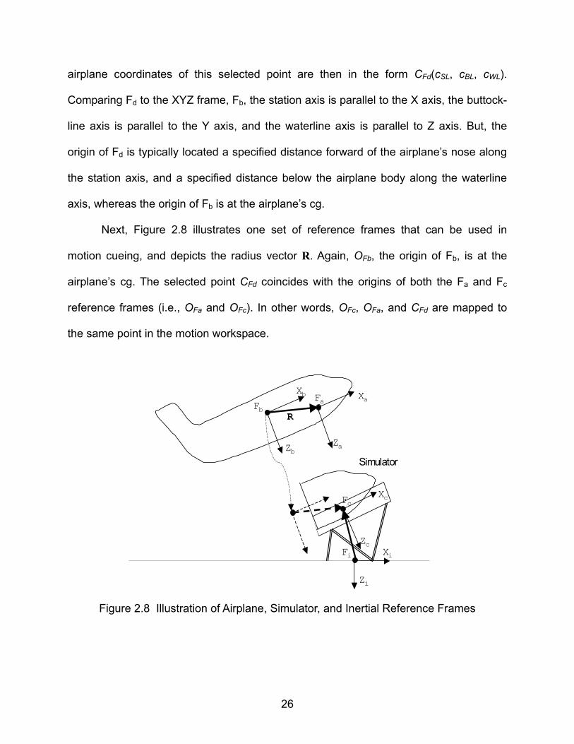
Next, Figure 2.8 illustrates one set of reference frames that can be used in
motion cueing, and depicts the radius vector R. Again, OFb, the origin of Fb, is at the
airplane’s cg. The selected point CFd coincides with the origins of both the Fa and Fc
reference frames (i.e., OFa and OFc). In other words, OFc, OFa, and CFd are mapped to
the same point in the motion workspace.
Fi
Fb R
Zi
Fc
Fa
Xi
Xc
Zc
Xa
ZaZb
Xb
Simulator
Figure 2.8 Illustration of Airplane, Simulator, and Inertial Reference Frames
26

The Y axes of all frames in Figure 2.8 are out of the page. Also, the relevance of
the inertial reference frame Fi will be explained later in conjunction with the motion
cueing component.
Finally, knowing the coordinates of CFd, the radius vector R can be defined by
locating the other endpoint, which is the location of the cg. The cg varies depending on
the operational configuration of the airplane. So, a nominal operating cg must be used.
Given the airplane’s wing mean aerodynamic chord (MAC), a nominal operating cg in
units of % MAC, and the airplane coordinates of the 0% MAC point, the coordinates of
the cg, CGFd(cgSL, cgBL, cgWL), can be found in the Fd frame. Then, R is represented by
the directed line segment CGFd CFd :
kjiR
kjiR
ZYX RRR ++=
−+−+−== )()()( WLWLBLBLSLSLFdFd ccgccgccgC CG (2-12)
where, for a B737-100 Airplane,(15) RX is 12.192 m, RY is 0.2286 m, and RZ is 1.74 m.
Therefore, these components of R are the required parameters in equation (2-10).
The definition of the transformation of the specific force vector fcg from the cg to
the centroid of the motion platform is complete. Whereas, in equation (2-9), the
subscript c meant an alternate location within the airplane, it is now synonymous with
the motion centroid using the components of R.
2.2.2 Motion Cueing Component
The motion cueing component computes the translational and rotational platform
position commands by scaling, transforming, and filtering the primary input signals from
27

the input component. It incorporates a common adaptive motion cueing algorithm, which
is based on the original method introduced by Parrish et al.(12) along with subsequent
developments.(14,15,20,27) Adaptive filters are used instead of linear ones in an effort to
optimize the cues. Filter parameters are continuously adjusted to minimize objective
functions through steepest descent methods in an attempt to provide the best possible
cues within the motion workspace. Figure 2.9 is an expanded block diagram
representing the motion cueing component in Figure 2.5.
ω
fc Scale and Limit
Scale and Limit
Body to InertialFrame Transfomation
Body Rates to Inertial Euler Rates Transfomation
TranslationalAdaptive Filters
RotationalAdaptive Filters
Integration
Integration
Position CommandsTo
Actuator ExtensionTransformation
X,Y,ZTranslational
PositionCommands
( surge, sway,and heave)
θ, φ, ψRotationalPosition
Commands(pitch, roll,and yaw)
ADAPTIVE MOTION CUEING
Transformed specific force
& Rotational velocity
inputs fromflight dynamics
Note: This cross-feed used to coordinatesurge-pitch and sway-roll cues, but notused for heave and yaw sincecoordination is not applicable.
Angular Position(θ, φ, ψ) Feedback forFrame Transformation
Figure 2.9 Block Diagram of the Motion Cueing Component
(Adapted from Reference 15)
The algorithm also coordinates the rotational and translational motions of the
platform in four DOF by combining parts of the translational and rotational channels to
achieve accurate longitudinal and lateral motion cues. Although the original method
28

used adaptive filters for four of the six DOF, the method was extended to all six DOF in
the subsequent developments.
The primary inputs to the motion cueing component, fcg and ω, were explained in
the previous section. So, the description starts with the scaling and limiting blocks.
2.2.2.1 Scaling and Limiting
The components of the specific force vector fc (fx,c,o, fy,c,o, fz,c,o) and the rotational velocity
vector ω (P, Q, R) are first scaled and limited to account for the performance limitations
of the motion system. The scaled vectors are the fc′ and ω′. For example, the scaling
and limiting function for the X-axis specific force fx,c,o is illustrated in Figure 2.10 and
described by
<+−>−−≤
=
1,,1,,,,,,
1,,1,,,,,,
1,,,,,
,
,)(7.0,)(7.0,
XfXfSfSXfXfSfSXffS
f
ocxocxoxocxox
ocxocxoxocxox
ocxocxox
cx (2-13)
where Sx,o is the scale factor, X1 is the function breakpoint, and fx,c is the function output.
As noted in the Figure 2.10, the scale factor is 0.5, and the breakpoint is 3.66 m/s2, or
0.37 g. All components are fed through this type of function, but the values of the scale
factor and breakpoint are unique for each component and depend on the limitations of
the corresponding degree of freedom. The specific force fc is limited to ±10 m/s2 and the
rotational velocity ω is limited to ±57.3 deg/s.
29

-10 -8 -6 -4 -2 0 2 4 6 8 10-3
-2
-1
0
1
2
3
fx,c,o
f x,c
X1=3.66,Sx,o=0.5
Figure 2.10 Scaling and Limiting Function for fx,c,o
An additional modification is made to the Z-axis specific force component before
it is fed through the scaling and limiting function. During steady-state level flight, the Z-
axis specific force is approximately –1g (-9.81 m/s2). That is, the lift force equals the
airplane weight, and so the specific force measured by the Z-axis accelerometer is
approximately –1g. The adaptive high pass filters ultimately filter out this low frequency
component of the Z-axis specific force. But, at this point, it must be removed in order to
properly scale and limit the pertinent high frequency components about 0 g. This is done
by adding 1 g to fz,c,o, scaling and limiting this quantity, then removing 1 g as follows:
30

fz,c = K(fz,c,o + 1) – 1 (2-14)
where K( • ) is the scaling and limiting function described by equation (2-13).
2.2.2.2 Frame Transformations
After scaling and limiting the components of fc and ω, fc′ and ω′ are transformed from the
airplane reference frame to an inertial reference frame. The coordinate system that
coincides with an inertial frame is depicted in Figure 2.8 as Fi. Fi is Earth-fixed and right-
handed with its Z-axis aligned with g. It is parallel to Fc with a collinear Z-axis when the
motion platform is at its neutral point and level. This frame is more convenient for driving
a motion platform, and as a result, it is the frame normally used in practice for this
purpose. There are a number of ways to perform this frame transformation, but the most
common(30) uses Euler angles. The Euler angles form the elements of the
transformation matrices that transform the specific force and rotational velocity vectors
between the simulator and inertial frames.
The transformation from one frame to another can be accomplished by three
successive rotations in a specific sequence. Using the Fc and Fi frames already defined,
the specific sequence of rotations, starting from Fc, follows the convention (28) used in
the airplane industry:
1. Rotate about the X-axis; right wing down yields a positive roll angle, φ.
2. Rotate about the new Y-axis; nose up yields a positive pitch angle, θ.
3. Rotate about the new Z-axis; nose right yields a positive yaw angle, ψ.
These rotations define the angles φ, θ, and ψ, known as the Euler angles. The
elements of the transformation matrices can now be expressed in terms of them. The
31

transformation matrix for the specific force will be covered first, followed by the one for
the rotational velocity.
The complete transformation of the specific force can be written as a product of
the individual rotation matrices, in the same sequence just described, as
fi = Bψ Bθ Bφ fc′ (2-15)
where
fc′ = [ fx,c fy,c fz,c]t - the body frame specific force vector (t - transpose),
fi = [fx,i fy,i fz,i]t - the inertial frame specific force vector(t - transpose),
−=
φφφφφ
cossin0sincos0
001B - the rotation matrix about the X-axis, through angle φ,
−=
θθ
θθ
θ
cos0sin010
sin0cosB - the rotation matrix about the Y-axis, through angle θ,
−=
1000cossin0sincos
ψψψψ
ψB - the rotation matrix about the Z-axis, through angle ψ.
Writing equation (2-15) with these rotation matrices gives
fi
−
−
−=
φφφφ
θθ
θθψψψψ
cossin0sincos0
001
cos0sin010
sin0cos
1000cossin0sincos
fc′ (2-16)
Multiplying the matrices in equation (2-16) yields the complete 3x3 transformation matrix
32

fi
−
−
+
+
−
=
θφθφθψφ
ψθφψφ
ψθφψθ
ψφψθφ
ψφψθφ
ψθ
coscoscossinsincossin
sinsincoscoscos
sinsinsinsincos
sinsincossincos
sincoscossinsin
coscos
fc′ (2-17)
which is written in compact form as
fi = B fc′ (2-18)
where the complete transformation matrix B is equal to Bψ Bθ Bφ. Note that B is
orthogonal and therefore
B-1 = Bt (2-19)
The specific force fi is finally converted to acceleration, before filtering, by
adding the gravitational force in the inertial frame
ai = fi + gi (2-20)
where gi = [0 0 1.]t in units of g. Converting the specific force to acceleration in the
inertial frame in this manner has some advantages.(7) Note that substituting equations
(2-14) and (2-18) into (2-20) yields
ai = B fc′ + gi = B{Kfc + (K-1)gi} + gi (2-21)
Regarding the first term B{Kfc + (K-1)gi}, recall that in order to properly scale and limit
the pertinent high frequency components about 0 g, gi was added to offset the Z-axis
33

specific force of approximately –1g, and then removed after scaling. The acceleration is
then computed in the inertial frame by adding gi to the transformed specific forces.
Alternatively, the acceleration could have been computed by adding gravity to the
specific force in the body frame as follows
ai = B {K(fc + B-1 gi)} (2-22)
But note that anomalous attitude-dependent forces will be introduced in the inertial
frame. This completes the transformation matrix for the specific force.
The rotational velocity vector is transformed to the inertial frame using the Euler
angles and their time derivatives. First, to establish the relationship between the Euler
angle rates and the components of the body rotational velocity, recognize that the
following equality (30) must hold:
φθψω ++=++= kji RQP (2-23)
Next, using the rotation matrices in equation (2-15) and following the reverse sequence
of successive rotations (i.e., from inertial to body frame, the sequence is yaw, pitch, and
roll), the components(28) of ω with respect to the body frame are
⋅
−
−=
ψθφ
θφφθφφ
θ
coscossin0cossincos0
sin01
RQP
(2-24)
or
Φω ET= (2-25)
34

where TE is the inertial-to-body frame transformation matrix, and Φ = [φ θ ψ]t. Then, to
transform ω′ to the inertial frame, equation (2-25) is inverted to express the inertial Euler
angle rates in terms of the body rotational velocities through the Euler angles of the
platform as
Φ (2-26) ω′= −1
ET
where
−=−
θφθφ
φφ
θφθφ
seccossecsin0
sincos0
tancostansin1
1ET (2-27)
The transformation matrix for the rotational velocity vector is complete.
2.2.2.3 Adaptive Filtering
After ai and are transformed from fΦ c′ and ω′, the next step is to pass them through
adaptive filters. First, note that Figure 2.9 can be viewed as three distinct block
diagrams of the adaptive cueing algorithm since the inputs are 3-D vectors: 1) the
longitudinal coordinated algorithm, 2) the lateral coordinated algorithm, and 3) the
directional/vertical algorithm. Of the six DOF, four are coordinated. The longitudinal
algorithm coordinates surge and pitch commands (X and θ), and the lateral algorithm
coordinates sway and roll commands (Y and φ). The directional, or yaw (ψ), commands
35

and the vertical, or heave (Z), commands are independent. All commands are adaptively
filtered.
The design of the adaptive filters is based on optimization methods.(50) In
particular, a parameter optimization method for dynamic systems is used.(49) The
dynamic systems in this case are the adaptive filters. Coordination is accomplished by
properly combining the translational acceleration with the rotational velocity in the
rotational channel. The concept of coordination is examined further while discussing the
structure of the adaptive filters. The structure of the longitudinal coordinated adaptive
filter is discussed first. Before going on though, a couple of points must be made here
about the adaptive filters to avoid confusion. First, the author claims no credit for the
design of these filters. The authors of a previous study(12) applied optimization methods
to design these adaptive filters, which are explained here for the reader’s understanding
since they are incorporated in the off-line motion simulation. Second, the minimization of
the adaptive filter objective functions via steepest descent techniques has no relation to
the objective function and steepest descent technique used to determine the dynamic
workspace limits in this research.
The form of the longitudinal coordinated filter is based on the notion of cue
coordination, which was introduced in a previous study(7) as a way to provide more
accurate longitudinal and lateral motion cues. In that study, linear, not adaptive, washout
filters were used, but false cues were a problem with this type of filter.(14,39)
Subsequently, adaptive washout filters(12) were introduced to further improve the motion
cues. In this approach, filter parameters are adjusted in real time using gradient
algorithms to present as much of a cue as possible within the workspace of the motion
36

system, while minimizing false cues. The co-filtering of the surge acceleration and pitch
velocity is coordinated so that initial surge of the platform is washed out after the pitch
channel sufficiently tilts the platform. This coordinated tilt aligns the gravity vector to
simulate a sustained longitudinal acceleration cue. Likewise, surge motion can be used
to counteract the false cues caused by the brief misalignment of the gravity vector
during pitch motion.
The longitudinal filter is primarily composed of the filter dynamics, the objective
function, and the steepest descent and sensitivity equations. The filter dynamics are
axxix
xxxix
a
XeXdaX
θδγθ
λ
+=
−−=
,
, (2-28)
and the associated objective function Jx ,
( ) ( ) 2222, 2222
1 XcXbWXaJ xxa
xxix ++−+−= θθ (2-29)
is minimized by defining the steepest descent for the adaptive parameters λx and δx as
( )
( )xxxix
xxx
xxxix
xxx
KJ
K
KJ
K
δδδ
δ
λλλ
λ
δδ
λλ
−+∂∂
−=
−+∂∂
−=
)0(
)0(
,,,
,,,
(2-30)
where
a i,x - adaptive filter input: inertial X-axis acceleration command,
XX , - adaptive filter state variables: inertial surge rate and acceleration,
X - adaptive filter output: uncompensated inertial platform surge position command,
37

aθ - adaptive filter input: inertial pitch rate command,
θ - adaptive filter state variable: inertial pitch rate,
θ - adaptive filter output: uncompensated inertial platform pitch command,
dx - adaptive filter: damping parameter for second order longitudinal washout,
ex - adaptive filter: frequency parameter for second order longitudinal washout,
λx - adaptive filter: surge adaptive gain (λx(0) – initial value at time, t = 0),
δx - adaptive filter: pitch rate adaptive gain (δx (0) – initial value at time, t = 0),
γx - adaptive filter: tilt coordination gains for sustained X-axis acceleration,
bx - objective function: weighted coefficient of the surge position penalty term,
cx - objective function: weighted coefficient of the surge rate penalty term,
Wx- objective function: weighted coefficient of the pitch rate error term,
Kλ,x, Kδ,x, Ki,λ,x , Ki,δ,x – steepest descent step sizes.
The gradients of the objective function for the steepest descent are expressed as
( )x
xx
xx
xix
x XXcXXbXaXJ
λλλλ ∂∂
+∂∂
+∂∂
−=∂∂
, (2-31)
( ) ( )x
xx
xx
axxx
xixi
x
x XXcXXbWXaXa
Jδδδ
θθθδδδ ∂
∂+
∂∂
+∂∂
−−
∂∂
−∂
∂−=
∂∂ ,
, (2-32)
and the corresponding equations for the sensitivity coefficients are
xx
xxxi
x
XeXdaXλλλ ∂
∂−
∂∂
⋅−=∂∂
, (2-33)
38

xx
xx
x
xix
x
XeXdaX
δδδλ
δ ∂∂
−∂∂
−∂
∂⋅=
∂∂ , (2-34)
ax
xix
x
aθ
δγ
δθ
+∂
∂=
∂∂ , (2-35)
x
xi
x
xi aaδθ
θδ ∂∂
∂
∂=
∂
∂ ,, (2-36)
( ) ( )
( ) cz
cycxxif
ffa
,
,,,coscoscos
sincoscoscossinφψθ
φψθψθθ +
+−=
∂
∂ (2-37)
And lastly for the longitudinal filter, the adaptive parameters are limited.
min,
min,
max,min,
max,min,
xx
xx
xxx
xxx
δδ
λλ
δδδ
λλλ
≥
≥
≤≤
≤≤
(2-38)
All parameters of the filter in equation (2-28) are constants except for the
adaptive gains λx, acceleration gain, and δx, pitch rate gain. These gains are adjusted in
real time in an attempt to minimize the objective function given in equation (2-29). The
objective function is composed of two tracking terms and two penalty terms. The gains
are adjusted in an effort to make the platform acceleration and pitch rate track the
acceleration and pitch rate commands, respectively, while constraining the platform
motion within the workspace with the platform position and rate penalty terms. Also,
note in equation (2-28) that the acceleration command is cross fed into the pitch
channel filter for tilt coordination. Tilt coordination will be explained and illustrated further
39

in the simulation examples of section 3.4.2. But, suffice it to say at this point, that tilt
coordination occurs because of the dependence of the acceleration command on the
platform pitch attitude in the pitch channel. During the onset of the surge acceleration
cue, the low frequency portion of the acceleration drives platform pitch rate until the
pitch channel aligns the gravity vector, providing the sustained acceleration effect, and
nulling the γxai,x term. Additional penalty terms are used in the steepest descent
equations, like Ki,λ,x(λx(0) - λx) in equation (2-30), to return the adaptive gains to their
original values after cues subside. The other filters perform in a similar manner and will
not be discussed.
The adaptive parameters in the sensitivity equations are assumed to be
independent. And, it is assumed that the derivatives exist and are continuous.(49) As
such,
xxx
XXdtd
dtXd
λλλ ∂∂
=
∂∂
=
∂∂
2
2
2
2
(2-39)
Some assumptions are also made about the derivatives involving platform Euler angles
that arise when obtaining the longitudinal sensitivity equations. First, derivatives
containing roll φ and yaw ψ Euler angles (lateral and directional quantities) are equal to
zero in the longitudinal channel,
0=∂∂
=∂∂
=∂∂
=∂∂
xxxx λψ
λφ
δψ
δφ (2-40)
Second, the derivative of Euler pitch angle with respect to λx is zero in the longitudinal
channel,
40

0=∂∂
xλθ (2-41)
Note that similar assumptions also apply to the coordinated lateral, directional, and
vertical adaptive filters that will be described.
The form of the lateral coordinated adaptive filter is the same as the longitudinal
one. The filter dynamics are
ayyiy
yyyiy
a
YeYdaY
φδγφ
λ
+−=
−−=
,
, (2-42)
and the associated objective function Jy,
( ) ( ) 2222, 2222
1 Yc
YbW
YaJ yya
yyiy ++−+−= φφ (2-43)
is minimized by defining the steepest descent for the adaptive parameters λy and δy as
( )
( )yyyiy
yyy
yyyiy
yyy
KJ
K
KJ
K
δδδ
δ
λλλ
λ
δδ
λλ
−+∂
∂−=
−+∂
∂−=
)0(
)0(
,,,
,,,
(2-44)
where
a i,y - adaptive filter input: inertial Y-axis acceleration command,
YY , - adaptive filter state variables: inertial sway rate and acceleration,
Y- adaptive filter output: uncompensated inertial platform sway position command,
aφ - adaptive filter input: inertial roll rate command,
41

φ - adaptive filter state variable: inertial roll rate,
φ - adaptive filter output: uncompensated inertial platform roll command,
dy - adaptive filter: damping parameter for second order lateral washout,
ey - adaptive filter: frequency parameter for second order lateral washout,
λy - adaptive filter: sway adaptive gain (λy(0) – initial value at time, t = 0),
δy - adaptive filter: roll rate adaptive gain (δy (0) – initial value at time, t = 0),
γy - adaptive filter: tilt coordination gains for sustained Y-axis acceleration,
by - objective function: weighted coefficient of the sway position penalty term,
cy - objective function: weighted coefficient of the sway rate penalty term,
Wy- objective function: weighted coefficient of the roll rate error term,
Kλ,y, Kδ,y, Ki,λ,y , Ki,δ,y – steepest descent step sizes.
The gradients of the objective function for the steepest descent are expressed as
( )y
yy
yy
yiy
y YYcYYbYaYJ
λλλλ ∂∂
+∂∂
+∂∂
−=∂
∂, (2-45)
( ) ( )y
yy
yy
ayyy
yiyi
y
y YYcYYbWYaYa
Jδδδ
φφφδδδ ∂
∂+
∂∂
+∂∂
−−
∂∂
−∂∂
−=∂∂ ,
, (2-46)
and the corresponding equations for the sensitivity coefficients are
yy
yyyi
y
YeYdaYλλλ ∂
∂−
∂∂
−=∂∂
, (2-47)
42

yy
yy
y
yiy
y
YeYdaY
δδδλ
δ ∂∂
−∂∂
−∂∂
=∂∂ , (2-48)
ay
yiy
y
aφ
δγ
δφ
+∂∂
−=∂∂ , (2-49)
y
yi
y
yi aaδφ
φδ ∂∂
∂∂
=∂∂ ,, (2-50)
( )( cz
cyyi
ffa
,
,,
sinsinsincoscoscossincossinsin
φψθψφ )ψφφψθ
φ +−−
=∂
∂ (2-51)
Like the longitudinal filter, the lateral adaptive parameters are limited.
min,
min,
max,min,
max,min,
yy
yy
yyy
yyy
δδ
λλ
δδδ
λλλ
≥
≥
≤≤
≤≤
(2-52)
The following assumptions, which are similar to those made for the longitudinal
filter, apply to the lateral filter:
• the adaptive parameters in the sensitivity equations are independent.
• the derivatives exist and are continuous.
• derivatives containing pitch θ and yaw ψ Euler angles (longitudinal and directional
quantities) are equal to zero in the lateral channel:
0=∂∂
=∂∂
=∂∂
=∂∂
yyyy λψ
λθ
δψ
δθ (2-53)
43

• the derivative of φ with respect to λy is zero in the lateral channel:
0=∂∂
yλφ (2-54)
The vertical and directional filters (heave and yaw) are not coordinated. They are
handled independently since the simulation of sustained acceleration via the alignment
of the gravity vector does not apply for these two DOF. Like the coordinated filters
though, they are composed of filter dynamics, an objective function, and steepest
descent and sensitivity equations.
The vertical adaptive filter is
ZeZdaZ zzziz −−= ,η (2-55)
and the associated objective function Jz,
( ) 222, 222
1 ZcZbzaJ zzziz ++−= (2-56)
is minimized by defining the steepest descent for the adaptive parameter ηz as
( zzziz
zzz KJK ηη
ηη ηη −+
∂∂
−= )0(,,, ) (2-57)
where
a i,z - adaptive filter input: inertial Z-axis acceleration command,
ZZ , - adaptive filter state variables: inertial heave rate and acceleration,
44

Z - adaptive filter output: uncompensated inertial platform heave position command,
dz - adaptive filter: damping parameter for second order vertical washout,
ez - adaptive filter: frequency parameter for second order vertical washout,
ηz - adaptive filter: heave adaptive gain (ηz (0) – initial value at time, t = 0),
bz - objective function: weighted coefficient of the heave position penalty term,
cz - objective function: weighted coefficient of the heave rate penalty term,
Kη,z , K i,η,,z - steepest descent step size.
The gradient of the objective function for the steepest descent is expressed as
( )z
zz
zz
ziz
z ZZcZZbZaZJηηηη ∂∂
+∂∂
+∂∂
−=∂∂
, (2-58)
and the corresponding equation for the sensitivity coefficient is
zz
zzzi
z
ZeZdaZηηη ∂∂
−∂∂
−=∂∂
, (2-59)
The limits on the vertical adaptive filter are
min,
max,min,
zz
zzz
ηη
ηηη
≥
≤≤ (2-60)
The directional adaptive filter is
ψψηψ ψψ ea −= (2-61)
and the associated objective function Jψ ,
45

( ) 22
221 ψψψ ψ
ψb
J a +−= (2-62)
is minimized by defining the steepest descent for the adaptive parameter ηψ as
( ψψψηψ
ψψηψ ηη
ηη −+
∂
∂−= )0(,,, iK
JK ) (2-63)
where
aψ - adaptive filter input: inertial yaw rate command,
ψ - adaptive filter state variable: inertial yaw rate,
ψ - adaptive filter output: uncompensated inertial platform yaw command,
ηψ - adaptive filter: yaw rate adaptive gain (ηψ (0) – initial value at time, t = 0),
bψ - objective function: weighted coefficient of the yaw position penalty term,
eψ - adaptive filter: frequency parameter for first order yaw washout,
Kη,ψ , Ki,η,ψ - steepest descent step sizes.
The gradient of the objective function for the steepest descent is expressed as
( )ψ
ψψψ
ψ
ηψψ
ηψψψ
η ∂∂
+∂∂
−=∂
∂b
Ja (2-64)
and the corresponding equation for the sensitivity coefficient is
ψψ
ψ ηψψ
ηψ
∂∂
⋅−=∂∂ ea (2-65)
46

The limits on the directional adaptive parameter are
min,
max,min,
ψψ
ψψψ
ηη
ηηη
≥
≤≤ (2-66)
It is assumed that the derivatives exist and are continuous for both the vertical and the
directional filter.
This concludes the description of the adaptive filtering. The integration of the
filters’ differential equations is now discussed.
2.2.2.4 Integration
Integration is the final step in the motion cueing component. Once the differential
equations for all of the filters are computed in the proper order, all derivatives are
integrated. The numerical computations of the longitudinal filter equations are used to
explain the process.
The pertinent longitudinal filter equations are (2-28) through (2-38). The
adaptive filter equation (2-28) is computed first followed by the state sensitivity
equations (2-37), (2-36), and (2-33) through (2-35). Next, equations (2-31) and (2-32),
the gradients of the objective function, are computed. And finally, the steepest descent
parameters in equation (2-30) are computed and limited. The equations for the other
adaptive filters are processed in a similar manner.
Note that the values of all filter parameters, like Kλ,j, Kδ,j, Ki,λ,j, Ki,δ,j, dj, ej, γj, bj, cj,
and Wj, where j is x, y, z, or ψ, must be selected. The values are based on both the
desired platform response and the workspace constraints. No attempt will be made to
47

discuss how the values are selected since it is fairly involved.(14,20,21,24) The parameter
values used are in Table 2.1.(15,27)
All derivatives must then be integrated. A second-order Adams-Bashforth-
Moulton (ABM) integration algorithm is used for the numerical integration. The ABM
method belongs to the class of linear multi-step methods (LMM) and is known to be
stable and accurate.(28) The integration uses a fixed time step equal to the reciprocal of
the iteration rate of the simulation. The iteration rate of the simulation is 30 Hz, which is
a common maximum rate in flight simulation.
Integration yields, among other parameters, the adaptive filter gains λj, δj, and ηj,
and the adaptive filter outputs, which are the platform position commands X, Y, Z, θ, φ,
and ψ. All platform position commands are sent to the motion actuator transformation
component.
48

Table 2.1 Values for the Adaptive Filter Parameters
Adaptive Filter, j (revised units)*Parameter j = x, y, z, or ψ Longitudinal, x Lateral, y Vertical, z Directional, ψ
Kλ,j (s3⋅m-2) 0.3229173125 0.516668 -- --Kδ,j (s3⋅m-2) 0.0107639104 0.269098 -- --Ki,λ,j (s-1) 0.02 0.05 -- --Ki,δ,j (s-1) 0.5 1.5 -- -- dj (s-1) 0.707 1.2727 1.2727 -- ej (s-2) 0.25 0.81 0.81 0.3 (s-1)* γj (s⋅m-1) 0.1640419948 0.1640419948 -- --bj (s-4) 0.01 0.1 0.1 1.0 (s-2)* cj (s-2) 0.2 2.0 0.1 -- Wj (m2⋅s-2) 0.00929 0.00929 -- --λj,min ( - ) -0.1 -0.1 -- --λj,max ( - ) 1.0 0.8 -- --d(λj,min)/dt (s-1) -0.06 -0.06 -- --λj(0) ( - ) 1.0 0.8 -- --δ j,min ( - ) 0.0 0.0 -- --δ j,max ( - ) 1.0 0.3 -- --d(δ j,min)/dt (s-1) -1000.0 -0.2 -- --δ j(0) ( - ) 0.5 0.3 -- --Kη,j (s3⋅m-2) -- -- 0.516669 100.0 (s)* Ki,η,j (s-1) -- -- 0.05 0.1η j,min ( - ) -- -- 0.0 0.0η j,max ( - ) -- -- 0.25 1.0d(η j,min)/dt (s-1) -- -- -0.06 -0.4η j(0) ( - ) -- -- 0.25 1.0
2.2.3 Motion Actuator Transformation Component
The three translational and three rotational platform position commands are
transformed into extension commands for the six motion actuators by the actuator
transformation component. The transformation is required because a conventional 6-
DOF motion system is not directly driven by position commands. The system moves in
each DOF by the combination of actuator extensions. So, the position commands must
49

be transformed into the actuator extensions before the signals are sent to the motion
hardware. This transformation is based on a geometrical representation of the motion
system.(9)
Figure 2.11 shows the geometry of the 6-DOF synergistic motion system. Recall
that inertial frame Fi is parallel to simulator frame Fc with a collinear Z-axis when the
platform is at its neutral position. And the motion centroid is the origin of Fc. A vector
diagram of a single motion actuator i from this figure is depicted in Figure 2.12.
Figure 2.11 Motion System Geometry
(Adapted from Reference 20)
Using this diagram, a vector equation(9) can be written for i using the vector
relationships between origins of the reference frames. The equation must be written in
50
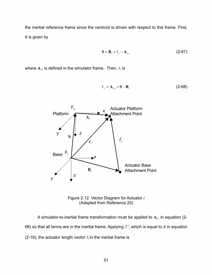
the inertial reference frame since the centroid is driven with respect to this frame. First,
S is given by
c i,ii ABS −+= (2-67)
where Ai,c is defined in the simulator frame. Then, i is
ic i,i BSA −+= (2-68)
yz
y z
x
xFc
FiBase
Platform
Actuator Base Attachment Point
Actuator Platform Attachment Point
i
Bi
Ai
ri
Si
Figure 2.12 Vector Diagram for Actuator i (Adapted from Reference 20)
A simulator-to-inertial frame transformation must be applied to Ai,c in equation (2-
68) so that all terms are in the inertial frame. Applying T t, which is equal to B in equation
(2-18), the actuator length vector i in the inertial frame is
51

(2-69) ii BSABSA −+=−+= ici,
ti T
where Ai,c and Bi are constants, and S is the vector representation of the translational
position commands X, Y, and Z that come from the motion cueing component. The
rotational commands enter the equation through T t. Ai,c and Bi are based on the
geometry of the motion system. In this study and demonstration, the values assigned to
Ai,c and Bi, which are listed in Table 2.1, were used in previous research.(15)
Table 2.2 Coordinates for the Actuator Attachment Points (Ai,z = 0.0; Select Bi,z for desired actuator quiescent point.)
Platform Attachment Points
Coordinates of Ai,c in Fc Base Attachment Points Coordinates of Bi in Fi
Actuator X coordinate
(meters) y coordinate
(meters) x coordinate
(meters) y coordinate
(meters) 1 2.1117 0.0762 1.5021 1.9812
2 2.1117 -0.0762 1.5021 -1.9812
3 -0.98986 -1.8669 0.96471 -2.29147
4 -1.12185 -1.7907 -2.46683 -0.31027
5 -1.12185 1.7907 -2.46683 0.31027
6 -0.98986 1.8669 0.96471 2.29147
As noted in Table 2.1, the actuators i can be driven about selected operating, or
quiescent, points (normally the same point for airplane simulators) depending on the
performance requirements. All position commands are null when the platform actuators
are in this quiescent state. When the actuators' quiescent points are one half of the their
total stroke, the actuators are at their neutral points. Thus, the platform is said to be in
52

the neutral position. Frequently, a constant offset from the platform neutral position is
used to achieve better pitch-up and heave performance. In this case, the actuators'
quiescent points are less than one half of the their total stroke. And the platform is said
to be in a depressed neutral position. A depressed neutral position is used in this study,
as was used in previous research.(15) So, Bi,z is selected to be 2.58064 m, where i=1-6,
for a desired actuator quiescent point of –0.145 m from the actuator's neutral point.
Dynamic offsets can also be applied to achieve the desired performance depending on
the simulator's mode of operation. Since extension, or length, commands for the
actuators are needed, the magnitude of i in equation (2-69) is required. The extension
command for actuator i is
L)( 2
1
−⋅= iit
i (2-70)
where L is a constant and is equal to the actuator neutral point when the platform is in
the neutral position. L is 3.38 m in this case given an actuator minimum length of 2.6162
m and a maximum length of 4.14 m.(9,15) Although the usable stroke for the actuators,
about the neutral point, is usually a little less than the maximum stroke due to hardware
protections (e.g., ± 0.6858 m), the total range of extension is
m762.0m762.0 ⋅+≤≤⋅− i , for i = 1 to 6 (2-71)
Finally, the extension commands are normalized to drive the analog hardware
)/(m762.0, FactorScaleADi
ni ⋅⋅×⋅
= , for i = 1 to 6 (2-72)
53

2.2.4 Motion Actuator Model Component
For the purpose of the demonstration, a simple actuator model is used to
simulate each of the six hydraulic actuators that are driven by the extension position
commands. The closed-loop frequency response of an actuator is derived using
frequency response analysis. A first-order low-pass model is identified based on
minimum motion performance requirements.(45) A 2.5 Hz break frequency is used to
sufficiently meet the system’s magnitude and phase requirements of greater than or
equal to –8 dB and –90 degrees, respectively, at 1.7 Hz. The actuator model is
71.15s71.15)s(G
i += (2-73)
In practice, lead compensation may be incorporated to meet tighter performance
requirements which specify an increased bandwidth.(10) This is not required for this
simulation demonstration.
2.3 Summary
This chapter provides sufficient background material on motion systems and
motion cueing to enable a better understanding of the issues that persist in the
evaluation of motion performance. Although much is known about motion cueing, the
motion system’s inherent inability to track inertial signals due to workspace constraints,
and its impact on perceptual fidelity, compound the difficulties in formulating objective
evaluation methods. In order to facilitate the development of evaluation methods, an off-
54

line motion system simulation is convenient. Thus, a math model that is the basis for a
simulation is furnished.
55

3.0 EVALUATION OF MOTION CUEING
3.1 Introduction
Now that the preparatory information on airplane simulator motion systems has
been presented, this chapter discusses the evaluation of the motion workspace and
motion cueing. It begins with a review of the current motion qualification criteria and the
related evaluation issues. Then, various techniques and concepts from previous motion
studies are presented as devices that can be used to make motion workspace and
cueing evaluation more effective. These devices are developed as needed for this
study, and incorporated into an improved evaluation method. The improvement is
demonstrated using the off-line motion system simulation that is based on the model
described in section 2.2.
3.2 Current Motion Qualification Criteria and Evaluation Issues
The current criteria for motion system validation are first reviewed. Then, the
issues concerning the criteria and evaluation are presented. These issues established
the basis for this research.
3.2.1 Current Motion Qualification Criteria
As previously mentioned, the current motion qualification criteria(1) are over
twenty years old. The criteria are based on a past standard(45) that focused more on the
56

specifications of motion hardware performance than on cueing performance and
evaluation. With the exception of validating the simulation of characteristic airframe
buffets, the current criteria, as applied by the industry, do not validate the integration of
the motion system with the flight dynamics simulation. The evaluation of the system is
done by testing it in a stand-alone mode to validate that it meets objective criteria for
hardware performance.
The stand-alone validation is composed of frequency response, actuator
balance, turn around, and transport delay tests. The frequency response characteristics,
magnitude and phase, are measured by driving all the motion actuators simultaneously
with a sinusoidal command signal that is generated by a sweep-frequency device over a
specified bandwidth. In most cases, this is only done for the vertical, or heave, axis. The
actuator balance characteristics are measured by driving the system in the heave mode
again with a sinusoidal command signal of a specified magnitude and frequency. The
actuators’ responses versus time are recorded. The maximum phase shift between any
two actuators must be within a specified percentage of the period of the command
signal. Next, the turn around characteristic is evaluated. The turn around bump of the
system is measured by driving it in the heave mode once more with a sinusoidal
command signal of a specified magnitude and frequency. The measured platform
acceleration versus time is evaluated by checking that the discontinuity in acceleration,
when the platform changes direction, is within the specified limits. These tests insure
that spurious motion due to deficient hardware is not perceivable.
Among the stand-alone tests, the transport delay test is closest to an integrated
test. It measures the system delays, apart from the simulated system dynamics, by
57

passing a flag, using a handshaking protocol, through all of the applicable system
interfaces and pertinent simulation modules from the control input to the system output
interfaces. The introduced transport delay through the simulator system must not
exceed a specified time delay. It also checks that the relative responses of the motion
system, visual system, and flight instrumentation to the step control input are closely
coupled to ensure, to some extent, the proper synchronization and integration of
sensory cues. The motion cue must occur before the visual cue for example. Recall the
psychophysical perception of motion discussed in section 2.1.3.
These stand-alone tests are essential as they provide a means of determining
the quality of the hardware, and to some degree, and indication that the hardware and
software are sufficiently integrated. They can expose the presence of hardware
anomalies that could adversely affect the pilot’s motion perception. But, obviously, the
motion workspace and cueing performance is not objectively checked. The tendency
has been to keep criteria simple and easy to apply. At the very least, the step response
of the cueing system could be checked during the transport delay test, but in most
cases either the motion dynamics are inhibited or the motion system is turned off
altogether.
3.2.2 Motion Evaluation Issues
Considering the importance of the motion system, it is not surprising that issues
arise when limited criteria are applied to such a complex system. More extensive and
appropriate integrated testing methods have been presented in past motion studies(11-14,
20-21, 40-43) that could be used to better assess cueing, but they have not been adopted in
58
general. There are several complicated problems(5, 35, 40-43) that persist mainly because
appropriate criteria are difficult to define.
A couple of outstanding issues that have not received a lot of attention involve
the workspace of the motion system. The workspace determines the cueing ability of the
motion system, and is therefore an important factor in motion fidelity. The outstanding
issues are how much of the workspace is being used during normal operation and what
amount of workspace is required to provide effective motion cues. The latter concern
involves complex human factors and will not be addressed here. The concern regarding
how much of, and how well, the workspace is being used is the focus of this study. For
example, it has been reported(2) that some motion systems appear to be attenuated to
the point of being ineffective. Another study(35) empirically examined the effect of
simulator motion on pilot training to determine if there is a sound basis for the motion
requirement to justify its cost. In this study, it was noted that the motion system did not
respond much to commanded vertical accelerations, especially during V1-cut(35)
maneuvers. Furthermore, lateral accelerations during rejected takeoffs and V1-cuts(35)
were not adequate.
There are a number of things that could cause the apparent deficiencies that
were observed in these studies. Factors like poor or improperly tuned cueing
algorithms, stricter performance and safety limits, improper cue integration and
synchronization, and workspace limitations are a few. In some cases, attenuation is
improperly used to mask false or negative cues due to a poorly designed motion cueing
system. Also, excursions in certain DOF restrict excursions in the others. Cues are then
limited in the restricted DOF. This might explain the inadequate lateral cues on V1 cuts
59

during which the simulator is in a pitch up attitude. In this case, a means of qualitatively
judging how well the workspace is being used, or the amount it is being restricted,
would be useful. A viable approach to evaluating the use of the workspace is presented
in the next section.
3.3 Motion Workspace Evaluation
Although the design of the motion system is intended to provide realistic motion
cues in six DOF, it is subject to performance limits. Of course, these limitations must be
considered when developing motion cueing algorithms. The motion platform cannot
exceed the position, velocity, and/or acceleration physical limits that are specified for
each degree of freedom.
The performance characteristics of a typical motion system are given in Table
3.1.(9,15) All of the limits are measured with respect to the platform quiescent position.
Recall from equation (2-70) that the actuator neutral point is 3.38 m. But, the platform
quiescent state is at a depressed neutral position as explained in section 2.2.3. All
position commands are null in the quiescent state. The motion system will provide single
degree of freedom excursions equal to the limits listed in the first row (See Note 1).
Since the maximum extension of an actuator is 4.14 m, an excursion in one DOF
reduces the maximum excursions that can be individually attained in each of the other
five DOF.
60

Table 3.1 Typical Motion Performance Limits (Adapted from Reference 9,15.)
Vertical Lateral Long-
ItudinalPitch Roll Yaw
Maximum Excursion
Up: 0.991 m Dn : 0.762 m
Left: 1.22 m Right : 1.22 m
Fwd: 1.24 m Aft: 1.22 m
Up: +30 ° (0.524 rad) Dn: -20 ° (-0.349 rad)
± 22 ° (± 0.384 rad)
± 32 ° (± 0.559 rad)
Maximum Velocity
± 0.61 m/s
± 0.61 m/s
± 0.61 m/s
± 15 °/s ± 15 °/s ± 15°/s
Maximum Acceleration
± 0.8g ± 0.6g ± 0.6g ± 50 °/s2 ± 50 °/s2 ± 50 °/s2
Notes:
1. The motion system will achieve the performance limits in a single-degree-of-freedom operation with an actuator quiescent point of -0.1459 m.
A previous study(11) empirically determined these excursion reductions for a
selected number of points on a particular system. It was explained that a motion
workspace for the system could not be readily described because of the infinite number
of possible combinations of excursions. Moreover, each DOF will allow a maximum
symmetric excursion in that DOF about its neutral point. The alternate neutral point also
affects the excursion limits.
Only excursion limit data for the interaction of two degrees of freedom were
collected and presented in tabular format. Effective motion cueing depends on sufficient
available excursion in all DOF. So, it would be useful when both tuning and evaluating
motion to record the actual platform trajectory in real-time so that the changing
excursion limits can be observed and analyzed temporally in all DOF. This then
motivates the development of a method that determines the dynamic excursion limits as
a function of the platform trajectory. This method is the focus of this study.
61

3.3.1 Motion Actuator Inverse Transformation
An important device that is used to develop a method to determine the dynamic
workspace limits is the motion actuator inverse transformation. This transformation was
presented in a previous study(9) to assist in the validation of hardware performance
(e.g., frequency response) by enabling the computation of the actual platform position,
in 6 DOF, based on the actuator extensions. The study also anticipated its use in the
feedback loop for optimal washout algorithms. Incidentally, the actuator extension
transformation that is presented in the section 2.2.3 also was presented in this study.
However, the transformation has been employed only on a limited basis. The
transformation incorporates the iterative Newton-Raphson Method(50) which requires a
variable amount of computational time based on the number of iterations needed to
reach a stopping criterion. Although fast converging, this somewhat indeterminate
method can cause problems in a real-time synchronous computing environment. When
used, it typically follows the actuator extension transformation to override and
decelerate the actuators as they approach the workspace limits. In some
applications,(11,13,14) the algorithm provides platform positions in all 6 DOF to a limit
prediction routine. The limit prediction routine then determines the nearest excursion
limits by solving for the pertinent roots of the quadratic expressions that are formed from
the actuator extension transformations. However, the limit prediction is only done for the
three translational DOF. Furthermore, in some configurations real roots might not exist.
In these cases, the solution is discarded. In another application,(27) the algorithm again
provides platform positions in all 6 DOF to an actuator braking routine. But, in this
62

instance, the braking routine uses the actual platform positions for comparison to the
commanded ones to determine how well the platform is tracking, in part, to control the
actuator deceleration. Limit prediction is done by other means.
So, before presenting the technique to determine the dynamic workspace limits,
this actuator inverse transformation is reviewed since it is a component of the new
technique. Actual platform position is typically difficult to determine unless the platform is
equipped with, say, a six-axis inertial measurement unit. The units are usually expensive
and still require some custom software to numerically compute the platform position
from the kinematical output signals.
An economical approach(9) is to compute the translational and rotational position
of the centroid of the platform from the magnitude of the actual actuator extensions, i.e.
the actuator inverse transformation. Each actuator’s extension is normally fed back to
the simulation host computer from its position transducer via the A/D interface. The
inverse transformation could be readily obtained if the actuator vectors i were available,
but the transducers only provide the magnitude of the actuator | i |. Therefore, the
problem is to solve six simultaneous nonlinear equations for the six unknown positions:
X, Y, Z, θ, φ, and ψ. The approach(9) is to apply an iterative numerical Newton-Raphson
method.(50) This method is a general method of computing the vector root α = [X, Y, Z, θ,
φ, ψ]t for the vector-matrix equation,
0f =)(α (3-1)
63

Then, according to Newton’s method, for a six-dimensional vector and six nonlinear
functions, the iteration formula has the form
)()(
1
nn
nn1n α
αα
αα ff
⋅
∂
∂−=
−
+ (3-2)
where [∂f(αn)/∂αn] is the Jacobian. A function satisfying the zeros vector in equation (3-1)
must now be defined to apply this method. Since the measured actuator extensions are
known, the function is defined as
2)(aii
tiif −=α (3-3)
where
=
φθψZYX
α (3-4)
=
)()()()()()(
)(
αααααα
α
6
5
4
3
2
1
ffffff
f (3-5)
64

and | i|a is the measured extension of actuator i which is obtained from the transducer.
Substituting equation (2-69) into equation (3-3), and multiplying the vectors yields a
scalar result. This enables the terms to be arranged as in equation (3-6). Recall that
transformation T t is equal to B.
2
2
2
222
)()()(
aiit
i
t
it
ci,tt
ici,tt
ci,t
ci,
ait
iit
ici,tt
iitt
ci,tt
it
ci,
t
ci,ci,tt
ci,
aiici,tt
ici,t
i
TT
T
TTTTT
TTf
−++
−−+=
−−+−−+
+−+=
−−+−+=
BBSS
BSABASAA
SBBBABBSSS
ASBASAAA
BSABSAα
(3-6)
Equation (3-7) is written by expanding equation (3-6) in terms of the elements
)(2
))((2
))((2
))((2
( 2222222222
zi,yi,xi,
33zc,i,23yc,i,13xc,i,zi,
32zc,i,22yc,i,12xc,i,yi,
31zc,i,21yc,i,11xc,i,xi,
aizi,yi,xi,zc,i,yc,i,xc,i,i
ZBYBXB
TATATABZ
TATATABY
TATATABX
ZYXBBBAAAf
++−
++−+
++−+
++−+
−++++++++=)α
(3-7)
65

Writing the partial derivatives of fi(α) in equation (3-7) with respect to the elements of
vector α yields
)(2)(
xi,31zc,i,21yc,i,11xc,i,i BTATATAXX
f−+++=
∂∂ α (3-8)
)(2)(
yi,32zc,i,22yc,i,12xc,i,i BTATATAYY
f−+++=
∂∂ α (3-9)
)(2)(
zi,33zc,i,23yc,i,13xc,i,i BTATATAZZ
f−+++=
∂∂ α (3-10)
))((2
))((2)(
31zc,i,21yc,i,11xc,i,yi,
32zc,i,22yc,i,12xc,i,xi,i
TATATABY
TATATABXψ
f
++−+
++−−=∂
∂ α
(3-11)
))(Z(2
))((2
))((2)(
sinθcosφA sinθsinφAcosθAB
sinψcosθ cosφA sinψcosθ sinφA sinψsinθABY
cosψ cosθ cosφAcosψ cosθ sinφAcosψ sinθABXθ
f
zc,i,yc,i,xc,i,zi,
zc,i,yc,i,xc,i,yi,
zc,i,yc,i,xc,i,xi,i
++−−
++−−+
++−−−=∂
∂ α
(3-12)
))((2
))((2
))((2)(
23zc,i,33yc,i,zi,
22zc,i,32yc,i,yi,
21zc,i,31yc,i,xi,i
TATABY
TATABY
TATABXφ
f
−−+
−−+
−−−=∂
∂ α
(3-13)
66
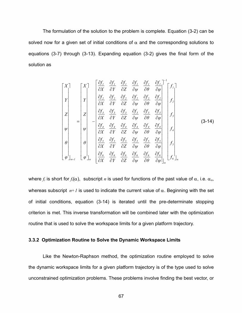
The formulation of the solution to the problem is complete. Equation (3-2) can be
solved now for a given set of initial conditions of α and the corresponding solutions to
equations (3-7) through (3-13). Expanding equation (3-2) gives the final form of the
solution as
n6
5
4
3
2
1
n
666666
555555
444444
333333
222222
111111
n1n f
f
f
f
f
f
φf
θf
ψf
Zf
Yf
Xf
φf
θf
ψf
Zf
Yf
Xf
φf
θf
ψf
Zf
Yf
Xf
φf
θf
ψf
Zf
Yf
Xf
φf
θf
ψf
Zf
Yf
Xf
φf
θf
ψf
Zf
Yf
Xf
φ
θ
ψ
Z
Y
X
φ
θ
ψ
Z
Y
X
∂∂
∂∂
∂∂
∂∂
∂∂
∂∂
∂∂
∂∂
∂∂
∂∂
∂∂
∂∂
∂∂
∂∂
∂∂
∂∂
∂∂
∂∂
∂∂
∂∂
∂∂
∂∂
∂∂
∂∂
∂∂
∂∂
∂∂
∂∂
∂∂
∂∂
∂∂
∂∂
∂∂
∂∂
∂∂
∂∂
−
=
−
+
1
(3-14)
where fi is short for fi(α), subscript n is used for functions of the past value of α, i.e. αn,
whereas subscript n+1 is used to indicate the current value of α. Beginning with the set
of initial conditions, equation (3-14) is iterated until the pre-determinate stopping
criterion is met. This inverse transformation will be combined later with the optimization
routine that is used to solve the workspace limits for a given platform trajectory.
3.3.2 Optimization Routine to Solve the Dynamic Workspace Limits
Like the Newton-Raphson method, the optimization routine employed to solve
the dynamic workspace limits for a given platform trajectory is of the type used to solve
unconstrained optimization problems. These problems involve finding the best vector, or
67

minimizer, x ∈ ℜn that minimizes the real-valued function, f(x), the objective function. It
is possible that other minimizers exist in these cases, but finding one minimizer suffices.
The optimization method is based on a steepest descent method using a constant step
size. The development, proof, and derivation of this algorithm are not presented in this
work. These particulars can be found in most texts on optimization methods.(50) Of
course, the specific implementation of the algorithm is described.
To determine the dynamic workspace limits for a given platform trajectory, the
steepest descent method is used in a stepwise manner to predict the workspace limits
for each degree of freedom, X, Y, Z, θ, φ, and ψ, throughout the trajectory. The algorithm
steps through each platform centroid position sample, αn=[Xn,Yn,Zn,θn,φn,ψn]t, in the
trajectory data. At each sample, the algorithm sequences through each of the six DOF
points within the sample, starting with Xn, while fixing the other five degrees of freedom
points to their values at that time. The specified maximum workspace limits, as in Table
3.1, for the current DOF being searched are selected for use in the steepest descent’s
quadratic objective function. The objective function is simply the squared difference of
the value of the current DOF point and the value of the current DOF excursion limit,
fn,i(αn,i ,αn,i,LIM) =(αn,i – αn,i,LIM)2, for i = 1,2,…,6 (3-15)
where i is the index for each DOF. The gradient of the objective function is then
∇fn,i(αn,i ,αn,i,LIM) = 2(αn,i – αn,i,LIM), for i = 1,2,…,6 (3-16)
The algorithm then starts a steepest descent search, first for the upper excursion
limit in the selected DOF, followed by a reversal in descent in order to seek the lower
68
excursion limit in the selected DOF. The descent is complete in either direction when the
stopping criteria is met. The stopping criteria are composed of normalized actuator
lengths, which were given in equation (2-72), an iteration limit in case the steepest
descent routine malfunctions, and the minimum acceptable limit on the gradient. Once
the upper and lower limits are determined for a selected DOF point within a sample, the
limits are stored, and the descent routine moves on to the next selected DOF point
within the sample. Thus, over all samples in the trajectory data, new limits are found and
stored for each DOF position point within a sample. The trajectory for each DOF is then
plotted along with its associated dynamic workspace limits for evaluation. Incidentally,
the upper and lower limit signals are filtered, without affecting their accuracy, to smooth
steps in the signals caused by the constant step size.
A little more must be said about the steepest descent routine regarding the
stopping criteria involving the actuator lengths. In order to check that a dynamic
excursion limit is not exceeded when descending in either direction, the normalized
actuator lengths are computed and used in the stopping criteria. The actuator lengths
are computed every iteration of the steepest descent search using the actual platform
trajectory. To do this, the actual actuator extension transformation component that is
described in section 2.2.3 is incorporated within the steepest descent routine. This
includes equations (2-69) through (2-70) and the coordinates that describe the platform
geometry. Recall that this component is used to drive the actuators in the normal real-
time motion simulation. An excursion limit is reached when the commanded position αn,i,
augmented by the iterative descent in the selected DOF, produces an actuator length
| i|(Xn=αn,i,Yn,Zn,θn,φn,ψn) that exceeds the usable actuator normalized length limits
69

specified in equations (2-71) and (2-72) . Unlike the previous study(11) in which limit
prediction is only done for the three translational DOF, this method does upper and
lower limit prediction in all six DOF. And, the issue of potential imaginary roots in the
limit prediction is not a factor. The flow chart of the steepest descent algorithm utilizing a
constant step size is listed in Figure 3.1.
70

Step 1. Display algorithm title.
Step 2. Clear workspace and initialize data (motion geometry, limits).
Step 3. Input the desired (constant) step size, αconstant.
Step 4. Select the desired trajectory: (0) for actual platform trajectory, or (1) for a constant attitude position trajectory.
Step 5. Load the trajectory data for the selection in Step 4.
Step 6. Start trajectory sample outer loop: sample n = 1: trajectory length
Step 7. Load trajectory sample αn=[Xn,Yn,Zn,θn,φn,ψn]t.
Step 8. Start intermediate loop for checking each DOF: axis = 1:6
Step 9. Load current axis limit αn,i,LIM into gradient term.
Step 10. Store trajectory sample αn into search limit buffer for refreshes.
Step 11. Start inner loop for each αn,i upper/lower limit: ullimit = 1:2
Step 12: Initialize search iteration index.
Step 13. Load current DOF sample αn,i into the gradient term.
Step 14. Compute the initial gradient, ∇fn,i(αn,i ,αn,i,LIM) = 2(αn,i – αn,i,LIM).
Step 15. Reset actuator extensions before each upper/lower limit search.
Step 16. Initialize the stopping criteria: usable normalized actuator limits, and maximum iteration count, and minimum gradient limit.
Step 17. While the stopping criteria is false, continue, else stop with limit and go
to Step 24. Step 18. Compute αn,i (k+1) = αn,i
(k) - αconstant∇fn,i(αn,i ,αn,i,LIM) (k) .
Figure 3.1 Steepest Descent Flow Chart for Dynamic Workspace Limits
71

Step 19. Increment the search iteration index.
Step 20. Update the gradient, ∇fn,i(αn,i ,αn,i,LIM), using αn,i (k+1)
Step 21. Store the current commanded descent position αn,i (k+1) into the current DOF search limit buffer.
Step 22. Compute the normalized actuator extensions using the platform
position, αn(k+1) , with the current commanded descent position αn,i (k+1).
The actuator extensions are computed using equations (2-69), (2-70), and (2-72).
Step 23. Go to Step 17 while any stopping criterion is false.
Step 24. Store the limit in the search limit buffer for the current DOF with the commanded descent position of αn,i (k+1). Index=1, upper limit; index=2, lower limit.
Step 25. Reverse sign on the current axis limit αn,i,LIM in the gradient to search in
opposite direction for the lower limit. Step 26. Go to Step 11 until the limits for the current αn,i of trajectory sample αn
are found. Step 27. Go to Step 8 until the limits for the six current αn,i positions of trajectory
sample αn are found. Step 28. Go to Step 6 until the limits for all of the trajectory samples αn are found. Step 29. Plot the trajectories for each DOF along with the its dynamic workspace
limits for evaluation. Filter the limits to smooth steps in the signals caused by the steepest descent step size.
Figure 3.1 (concluded)
This completes the design of the optimization routine for the dynamic workspace
limits. The performance of the algorithm is now checked.
72

3.3.3 Simulation Results and Discussion
The performance of the optimization routine for the dynamic workspace limits is
now checked before combining it with the actuator inverse transformation to evaluate
test trajectories. First, the performance of the steepest descent algorithm for one DOF is
demonstrated and evaluated to determine a good constant step size, in terms of
accuracy and speed. The upper and lower limits of the Z axis are plotted to observe the
effects of the step size. Figure 3.2 illustrates the search trajectory for the Z axis upper
limit. Figure 3.3 is the trajectory for the Z axis lower limit.
0 1 2 3 4 5 6 7 80
0.1
0.2
0.3
0.4
0.5
0.6
0.7
0.8
Z A
xis
Lim
it
Trajectory Sample n
Z Axis Workspace Limit Search Trajectory
Figure 3.2 Z Axis Upper Limit Search Trajectory
73

0 1 2 3 4 5 6 7 8 9-0.8
-0.6
-0.4
-0.2
0
0.2
0.4
0.6
0.8
Z A
xis
Lim
it
Trajectory Sample n
Z Axis Workspace Limit Search Trajectory
Figure 3.3 Z Axis Lower Limit Search Trajectory
The step size for this set of limits is chosen arbitrarily so that a comparison can made to
other step sizes. Figures 3.2 and 3.3 are just a sample of a large number of trajectories
that can be generated by adjusting the step size to achieve the various degrees of
accuracy in reaching the limits.
The constant step size used in Figures 3.2 and 3.3 is 0.1. The starting platform
position point is αn=[Xn,Yn,Zn,θn,φn,ψn]t = [0,0,0,0,0,0]. The upper limit for the Z axis is
located at about 0.75 m and the lower limit at approximately - 0.7 m. Note that the
convergence is quick and the limits are reached within 9 iterations. The step size is now
decreased to determine if a higher accuracy can be obtained.
A new step size of 0.01 yields the results in Figures 3.4 and 3.5. For the same
starting point αn = [0,0,0,0,0,0], the new Z axis limits are located at about 0.725 m for the
74

upper limit, and -0.65 m for the lower one. As expected, although the convergence is
still quick, the number of iterations required to reach the limits has increased tenfold.
0 10 20 30 40 50 60 70 800
0.1
0.2
0.3
0.4
0.5
0.6
0.7
0.8
Z A
xis
Lim
it
Trajectory Sample n
Z Axis Workspace Limit Search Trajectory
Figure 3.4 Z Axis Upper Limit Search Trajectory
75

0 10 20 30 40 50 60 70 80 90 100-0.8
-0.6
-0.4
-0.2
0
0.2
0.4
0.6
0.8
Z A
xis
Lim
it
Trajectory Sample n
Z Axis Workspace Limit Search Trajectory
Figure 3.5 Z Axis Lower Limit Search Trajectory
After several more test runs, it is fairly evident that the error is sufficiently
reduced at the limits using the step size of 0.01. Changes in the limits are not that
noticeable when decreasing the step size to 0.001, although the number of search
iterations increases significantly. For the purpose of demonstrating the improved
evaluation method, eyeballing the results in these figures to assess accuracy is
sufficient. When implementing this method, in part, to validate motion performance, a
higher degree of accuracy would be required. So, for the starting point αn = [0,0,0,0,0,0],
the Z axis limits are located at about 0.725 m for the upper limit, and -0.65 m for the
lower one.
After checking the limits in each DOF, the routine is used to evaluate the limits
in all DOF. Figure 3.6 presents the limits for all DOF in time history format. Translational
76

limits (X, Y, Z) are in meters, and rotational limits (Pitch, Roll, Yaw) are in radians.
Results in tabular format can also be produced if more accuracy is required.
0 0.5 1-1
0
1
2
X A
xis
Motion Workspace Limits - All Degrees of Freedom
0 0.5 1-1
0
1
Y A
xis
0 0.5 1-1
0
1
Z A
xis
Trajectory Time History, sec
0 0.5 1-0.5
0
0.5
Yaw
Axi
s
0 0.5 1-0.5
0
0.5
Pitc
h A
xis
0 0.5 1-0.5
0
0.5
Rol
l Axi
s
Trajectory Time History, sec
Figure 3.6 Motion Workspace Limits for αn = [0,0,0,0,0,0]
The platform is held in a steady state position of αn = [0,0,0,0,0,0] while the limits are
found using a step size of 0.01. Observe that all platform position traces are at zero, i.e.,
αn = [0,0,0,0,0,0], along with their corresponding upper and lower limit traces. These
results can be used to verify specific excursion limits of the motion system like those
listed in Table 3.1. This leads to an interesting issue regarding Table 3.1. The
77

geometrical data(15) that is used in the workspace routine is supposedly related to the
excursion limits in Table 3.1, but this is not conclusive. Therefore, the actual Z axis limits
should be approximately +0.99 m and –0.762 m at αn=[0,0,0,0,0,0]. Yet the algorithm
computed the limits to be about +0.725 m and -0.65 m. There are a lot of factors that
could cause these discrepancies, like the stopping criteria which incorporates the
actuator usable stroke in lieu of the maximum stroke, and a minimum gradient. Both the
data and the algorithm will need to be checked more thoroughly to resolve this issue.
Better yet, the algorithm should be calibrated, adjusted and checked on an actual
airplane simulator. However, this case suffices to show the potential of the routine.
Two more cases illustrating workspace limits in the steady state are examined,
but obviously, an infinite number of combinations exist. Figure 3.7 depicts the
workspace limits for a 1-meter excursion in just the X axis, αn=[1,0,0,0,0,0]. Figure 3.8
shows the limits for an X excursion of 0.5 m, and a pitch excursion of 0.2 rads,
αn=[0.5,0,0,0,0.2,0]. Both figures illustrate the considerable reductions that occur in the
other DOF when a displacement occurs in one or two others. Compare these results to
Figure 3.6. The results help one to better understand and appreciate how a significant
excursion in one or two axes can significantly decrease the motions ability to provide
effective cues in the others.
78

0 0.5 1-1
0
1
2
X A
xis
Motion Workspace Limits - All Degrees of Freedom
0 0.5 1-0.1
0
0.1
Y A
xis
0 0.5 1-0.04
-0.02
0
0.02
Z A
xis
Trajectory Time History, sec
0 0.5 1-0.02
0
0.02
Yaw
Axi
s
0 0.5 1-0.05
0
0.05
Pitc
h A
xis
0 0.5 1-0.02
0
0.02
Rol
l Axi
s
Trajectory Time History, sec
Figure 3.7 Motion Workspace Limits for αn = [1,0,0,0,0,0]
79

0 0.5 1-1
0
1
X A
xis
Motion Workspace Limits - All Degrees of Freedom
0 0.5 1-0.2
0
0.2
Y A
xis
0 0.5 1-0.1
0
0.1
Z A
xis
Trajectory Time History, sec
0 0.5 1-0.1
0
0.1
Yaw
Axi
s
0 0.5 1-0.5
0
0.5
Pitc
h A
xis
0 0.5 1-0.05
0
0.05
Rol
l Axi
s
Trajectory Time History, sec
Figure 3.8 Motion Workspace Limits for αn = [0.5,0,0,0,0.2,0]
In summary, a new technique for computing the limits of the motion workspace is
presented. It is based on steepest descent methods, and uses a constant step size.
Although using a constant step size is not as effective as using other techniques, it is
straightforward and easy to implement. And, since this study will propose that the
method be used to post process the motion trajectory data, in lieu of attempting to
integrate it into the real-time simulator environment, speed is not as important as
accuracy.
80

The Newton-Raphson method works well in the actuator inverse transformation
since the commanded platform position is usually very close to its current solution.
Newton-Raphson is known to have superior convergence when used in this manner.
But, when the starting points are far away from the solution, its convergence properties
can be poor.
The new routine will now be combined with the actuator inverse transformation to
provide a way to better judge the quality of motion cues within the workspace. The
improved method is demonstrated using the off-line motion system simulation.
3.4 Improved Method for Evaluating Motion Cueing
The off-line simulation of the motion system is now used to demonstrate how the
optimization routine for the workspace limits could be employed in a practical
application. Test signals that approximate typical airplane specific forces, for selected
maneuvers, are used to drive the simulation for each test run. A test run generates a
simulated actual platform trajectory that is recorded. The recorded data are processed
by the optimization routine to determine the dynamic workspace limits as a result of the
trajectory. The time history of the trajectory, including the limits, is plotted for evaluation.
It is shown that the inclusion of the limits is an improvement to the method used to
evaluate the quality of the motion cues within the motion workspace.
81

For reference, the flowchart for the off-line simulation is shown below.
• Test Sig
• Airplane• Airplane• Long., L• Integrat
• Rec*Note:
• Fin
Six Degrees-Of-Freedom Motion System Off-Line Simulation
Figure
One-Time Data Intialization
Interactive Input Component nal Selection and Iteration Rate
Scaling / Limiting Component
i
Motion Cueing Component Body to Inertial Transformation Body to Euler Rates Transformation ateral, Vert., & Direct. Adaptive Filters on
Actuator Extension Transformation Component
Platform Actuator Model Component
*Inverse Actuator Transformation Component ord Platform Trajectory : αn=[Xn,Yn,Zn,θn,φn,ψn]t Optional – Can Record Act. Ext. | i|(Xn,Yn,Zn,θn,φn,ψn)
N
Done?
Optimization Routine to Find Dynamic Workspace Limits d and plot Platform (optionally, Actuator) Trajectory & Limits
3.9 Flowchart for the Off-
82
Y
line Motion Simulation

Note that all of the simulations and results in this work are done with MATLAB,
Version 5.1, a PC-based high-performance language for technical computing by The
MathWorks, Inc.. MATLAB is used to program, interactively execute, and evaluate the
performance of all algorithms. In all flowcharts, each key step is given, but without a lot
of MATLAB-code detail. For example, algorithms may specify the output of certain
plots, but the details of the code involved with a plot, like plot spacing and range, axis
and plot labels, etc., are not given for the sake of clarity.
3.4.1 Combining Inverse Transformation and the Workspace Limits Routine
Before presenting the simulation results, the combination of the inverse
transformation and the workspace limits routine, in this study, are discussed briefly. As
shown in Figure 3.9, the actuator inverse transformation is combined with the pseudo
real-time simulation to record the platform trajectory after transforming the actuator
extensions into platform position. The flowchart box for the actuator inverse
transformation notes that the actuator extension trajectory can be recorded in lieu of the
platform trajectory. The reason for this is that the configuration of airplane simulator
motion simulations, old and new, may differ. So this method can be adapted to a
specific simulator implementation.
For example, recall the block diagram of the typical motion system that is shown
in Figure 2.5. Below are similar, but simplified, block diagrams that are used to explain
the implementation of the routines. In a lot of older simulators, the inverse actuator
extension component is not utilized. But, the capabilities exist to record the actuator
extensions in the real-time environment as shown in Figure 3.10. So in this case, it is
83

proposed that the inverse transformation and workspace limits routine be combined and
integrated into the simulator’s software environment, and used to post process the
recorded motion and associated test data, in lieu of attempting to integrate them into the
real-time simulator environment. This is shown in Figure 3.11. Alternatively, if the
platform position trajectory is recorded, the inverse transformation can be bypassed.
6 DOFMotion
ActuatorModel
MotionCueingSystem
Aerodynamic and MotionReal-Time Simulation
MotionActuator
ExtensionTransformation
andLead
Compensation
AirplaneSimulation:Equations
of Motion OutputSignals
MotionInputSignal
Transformation
INPUT/OUTPUT
INTERFACE
ActuatorDrive
Signals
ActuatorFeedbackSignals
i actual
i cmd
i = 1,..,6
RecordActuator
ExtensionsIn
RealTime
Figure 3.10 Simplified Motion Block Diagram
84

6 DOFMotion
ActuatorModel
MotionCueingSystem
Aerodynamic and MotionReal-Time Simulation
MotionActuator
ExtensionTransformation
andLead
Compensation
AirplaneSimulation:Equations
of Motion OutputSignals
MotionInputSignal
Transformation
INPUT/OUTPUT
INTERFACE
ActuatorDrive
Signals
ActuatorFeedbackSignals
i actual
i cmd
i = 1,..,6
RecordActuator
ExtensionsIn
RealTime
Post ProcessActuator
ExtensionsAnd
Related Signals
Figure 3.11 Motion Block Diagram with Motion Data Post Processing System
3.4.2 Simulation Results and Discussion
As described above, the off-line simulation, including the actuator inverse
transformation and the workspace limits routine, is implemented in MATLAB and run
on a standard Pentium-based PC. The simulated iteration rate is 15 Hz, so the time
step is 66.67 ms. Although run in a pseudo real time environment, it is sufficient to
demonstrate how the system could be employed in a practical application. All
components of the simulation have already been discussed in sufficient detail in
previous sections, with the exception of the generation of the test signals contained in
the input component. Test signals that approximate typical airplane rotational rates, ω,
85

and specific forces, fc, for selected maneuvers, can be used to drive the simulation.
Recall that fc and ω are the required inputs to the Motion System Input Component, as
explained in the section 2.2.1. But, for this demonstration, only specific forces, fc, are
used for each test case. The units used for fc are m/s2.
Test cases are selected to determine, in a preliminary manner, the performance
of the optimization algorithm for the workspace limits. Of course, a large number of test
cases could be demonstrated, but only a few which adequately illustrate the viability of
the routine are used. No attempt is made to evaluate the performance of any other
component by adjusting its parameters, i.e., the motion cueing component. This is
considered to be outside the scope of this work. Ample studies exist that can be
referenced for this information.
For each test run, the test signals for the selected case drive the simulation and a
simulated actual platform trajectory, αn=[Xn,Yn,Zn,θn,φn,ψn]t, is recorded. The optimization
routine that determines the dynamic workspace limits is then invoked. The routine
requests 1) the desired constant step size for the steepest descent search, 2) the stroke
limit of the actuator, and 3) whether the current platform trajectory or a single point is to
be processed. The recorded trajectory data are processed, and a time history of the
trajectory, including the upper and lower limits of the workspace, is plotted for
evaluation.
The first test case, test case 1, is now presented. Test case 1 is a longitudinal
translation (surge-pitch) demonstration. To demonstrate the viability of the workspace
limits routine, simple test signals that approximate typical airplane ω and fc, rather than
complex ones representing a complete airplane maneuver, are used. This makes the
86

evaluation easier for this preliminary study. For this case, the test signal is a
longitudinal specific force pulse.
fc = [fx fy fz]t = [(fx pulse) 0 –g]t (3-17)
Equation (3-17) represents an ideal response of the simulated airplane to either a thrust
pulse during takeoff or an airspeed change while flying straight and level. In a real-time
simulation environment, this signal would be provided to the motion input component by
the six-DOF equations-of-motion module in the flight dynamics simulation. Recall that
the Z-axis specific force component fz must be set to –g for the reasons discussed in
section 2.2.2.1, Scaling and Limiting. The magnitude of the fx pulse is 2.0 m/s2. This is a
good approximation to the acceleration of a typical commercial airplane.
The results of test case 1 are shown in Figures 3.12 and 3.13. First, note the
effects of the scaling and limiting component on the fx pulse in Figure 3.12. The pulse is
limited to about 1 m/s2, per equation (2-13), yielding the scaled specific force fx,c. As
explained in section 2.2.2.1, this scaling intentionally reduces the input magnitude in an
attempt to keep the motion from driving to its limits. The dashed line is fx,c. The plot for fz,
which is just –g, is not plotted.
87

0 5 10 15 20 25 30 35 40 45 50-0.5
0
0.5
1
1.5
2S
peci
fic F
orce
s f x ,
fx,
c and
Pla
tform
X A
ccel
.,
m/s
2
time, sec
Figure 3.12 Test Case 1: Specific Force Inputs and Platform X Acceleration
Also, the longitudinal adaptive state variable, platform acceleration X , is plotted along
with input signals for comparison. This illustrates the effect of the second order adaptive
washout filter. Platform acceleration is integrated to yield the platform surge position
command, X , which is shown in Figure 3.13.
One point must be made here. Usually, to assess the quality of motion cueing,
data on simulated airplane motions, airplane pilot sensations, simulator motions,
simulator pilot sensations, and motion platform positions are plotted, at a minimum.
More will be said about this additional data later. For this demonstration though, platform
positions are only plotted since the focus is on the workspace limits.
88

Figure 3.13 shows the actual platform positions along with the upper and lower
limits for each DOF versus time. The workspace limits are found using a constant step
size of 0.02.
0 20 40 60-1
0
1
2
X plat
form
, m
0 20 40 60-1
0
1
Ypl
atfo
rm,
m
0 20 40 60-1
0
1
Z plat
form
, m
Trajectory Time History, sec
0 20 40 60-50
0
50
Yaw
plat
form
, de
g
0 20 40 60-50
0
50P
itch pl
atfo
rm,
deg
<-- Tilt Target
0 20 40 60-50
0
50
Rol
l plat
form
, de
g
Trajectory Time History, sec
Figure 3.13 Test Case 1: Platform Positions and Workspace Limits
The trajectory sample length for test case 1 is 750 samples (samples = iteration rate*
trajectory time = 15 samples/sec * 50 sec). For the six DOF, the routine finds both the
upper and lower limits for 4,500 total samples. The processing time is about 2 minutes.
Since the test signal is composed of just a longitudinal specific force, the
operation of the longitudinal coordinated adaptive filter is easy to see. The generation of
89
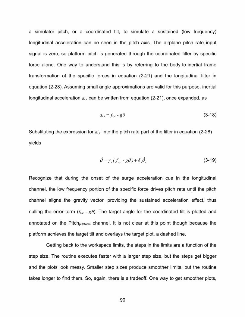
a simulator pitch, or a coordinated tilt, to simulate a sustained (low frequency)
longitudinal acceleration can be seen in the pitch axis. The airplane pitch rate input
signal is zero, so platform pitch is generated through the coordinated filter by specific
force alone. One way to understand this is by referring to the body-to-inertial frame
transformation of the specific forces in equation (2-21) and the longitudinal filter in
equation (2-28). Assuming small angle approximations are valid for this purpose, inertial
longitudinal acceleration ai,x can be written from equation (2-21), once expanded, as
ai,x = fx,c - gθ (3-18)
Substituting the expression for ai,x into the pitch rate part of the filter in equation (2-28)
yields
axx θδθγθ += )g - f( cx, (3-19)
Recognize that during the onset of the surge acceleration cue in the longitudinal
channel, the low frequency portion of the specific force drives pitch rate until the pitch
channel aligns the gravity vector, providing the sustained acceleration effect, thus
nulling the error term (fx,c - gθ). The target angle for the coordinated tilt is plotted and
annotated on the Pitchplatform channel. It is not clear at this point though because the
platform achieves the target tilt and overlays the target plot, a dashed line.
Getting back to the workspace limits, the steps in the limits are a function of the
step size. The routine executes faster with a larger step size, but the steps get bigger
and the plots look messy. Smaller step sizes produce smoother limits, but the routine
takes longer to find them. So, again, there is a tradeoff. One way to get smoother plots,
90

in a reasonable time, is to pass the limit signals through a low pass filter. The effect of
filtering the limits in this manner is shown in Figure 3.14 and Figure 3.15 for the Zplatform
signal. A first-order low pass filter is used with an empirically determined time constant.
The time constant must be carefully selected so that phase lags are not introduced. A
time constant of 0.5 seconds is used here. The unfiltered limits are shown along with the
filtered ones in Figure 3.14. In Figure 3.15, the unfiltered limits are removed to show the
end result. The choice of whether to use this technique or not will depend on the
application. Other methods could also be used.
0 5 10 15 20 25 30 35 40 45 50-0.8
-0.6
-0.4
-0.2
0
0.2
0.4
0.6
0.8
Z plat
form
, m
Trajectory Time History, sec
Figure 3.14 Unfiltered and Filtered Zplatform Limit Signals
91

0 5 10 15 20 25 30 35 40 45 50-0.8
-0.6
-0.4
-0.2
0
0.2
0.4
0.6
0.8
Z plat
form
, m
Trajec tory Tim e His tory , sec
Figure 3.15 Filtered Zplatform Limit Signals
Another test, which is similar to test case 1, is run. This test case is 1A. The
only difference is that the magnitude of the longitudinal specific force pulse is increased
by 50% to 3.0 m/s2. This test examines the effect of larger input signals on the
workspace limits. The results are shown in Figures 3.16 and 3.17 below. In Figure 3.16,
the fx pulse is again scaled by the scaling and limiting component. The resultant
magnitude of the scaled specific force fx,c is 1.5 m/s2. The dashed line is fx,c. The plot for
fz, which is just –g, is not plotted. The platform acceleration X is plotted along with input
signals for comparison.
92

0 5 10 15 20 25 30 35 40 45 50-1
-0.5
0
0.5
1
1.5
2
2.5
3
Spe
cific
For
ces
f x , f
x,c a
nd P
latfo
rm X
Acc
el.,
m
/s2
time, sec
Figure 3.16 Test Case 1A: Specific Force Inputs and Platform X Acceleration
It is clear in Figure 3.17 how a significant excursion in the X axis considerably
reduces the amount of available excursion in the other DOF. The pitch channel is still
able to achieve the target tilt angle though. However, if a subsequent cue is
commanded in any other DOF, especially yaw or roll, the platform would be unable to
respond properly. If the limits are not apparent, one might believe that sufficient travel is
still available in these DOF.
93
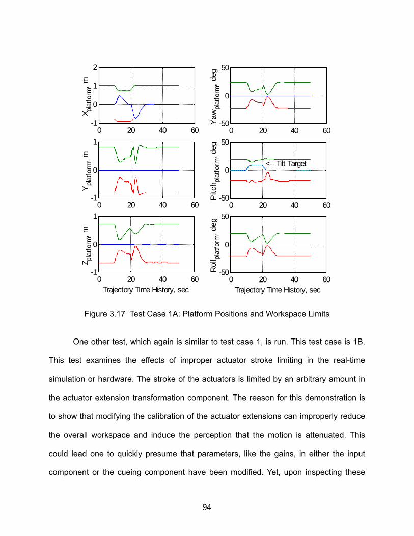
0 20 40 60-1
0
1
2
X plat
form
, m
0 20 40 60-1
0
1
Ypl
atfo
rm,
m
0 20 40 60-1
0
1
Z plat
form
, m
Trajectory Time History, sec
0 20 40 60-50
0
50
Yaw
plat
form
, de
g0 20 40 60
-50
0
50
Pitc
h plat
form
, de
g
<-- Tilt Target
0 20 40 60-50
0
50R
oll pl
atfo
rm,
deg
Trajectory Time History, sec
Figure 3.17 Test Case 1A: Platform Positions and Workspace Limits
One other test, which again is similar to test case 1, is run. This test case is 1B.
This test examines the effects of improper actuator stroke limiting in the real-time
simulation or hardware. The stroke of the actuators is limited by an arbitrary amount in
the actuator extension transformation component. The reason for this demonstration is
to show that modifying the calibration of the actuator extensions can improperly reduce
the overall workspace and induce the perception that the motion is attenuated. This
could lead one to quickly presume that parameters, like the gains, in either the input
component or the cueing component have been modified. Yet, upon inspecting these
94
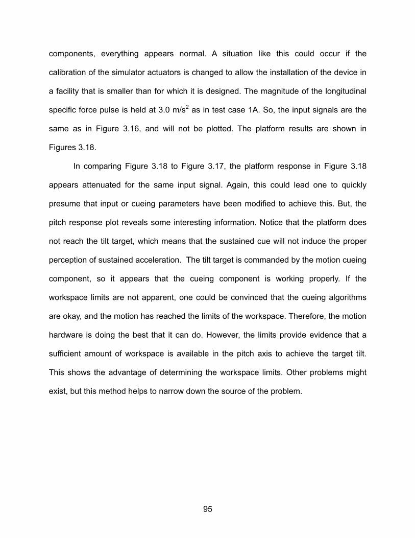
components, everything appears normal. A situation like this could occur if the
calibration of the simulator actuators is changed to allow the installation of the device in
a facility that is smaller than for which it is designed. The magnitude of the longitudinal
specific force pulse is held at 3.0 m/s2 as in test case 1A. So, the input signals are the
same as in Figure 3.16, and will not be plotted. The platform results are shown in
Figures 3.18.
In comparing Figure 3.18 to Figure 3.17, the platform response in Figure 3.18
appears attenuated for the same input signal. Again, this could lead one to quickly
presume that input or cueing parameters have been modified to achieve this. But, the
pitch response plot reveals some interesting information. Notice that the platform does
not reach the tilt target, which means that the sustained cue will not induce the proper
perception of sustained acceleration. The tilt target is commanded by the motion cueing
component, so it appears that the cueing component is working properly. If the
workspace limits are not apparent, one could be convinced that the cueing algorithms
are okay, and the motion has reached the limits of the workspace. Therefore, the motion
hardware is doing the best that it can do. However, the limits provide evidence that a
sufficient amount of workspace is available in the pitch axis to achieve the target tilt.
This shows the advantage of determining the workspace limits. Other problems might
exist, but this method helps to narrow down the source of the problem.
95

0 20 40 60-1
0
1
2
X plat
form
, m
0 20 40 60-1
0
1
Ypl
atfo
rm,
m
0 20 40 60-1
0
1
Z plat
form
, m
Trajectory Time History, sec
0 20 40 60-50
0
50
Yaw
plat
form
, de
g
0 20 40 60-50
0
50
Pitc
h plat
form
, de
g
<-- Tilt Target
0 20 40 60-50
0
50
Rol
l plat
form
, de
g
Trajectory Time History, sec
Figure 3.18 Test Case 1B: Platform Positions and Workspace Limits
96

4.0 DISCUSSION AND CONCLUSION
4.1 Discussion
Many factors affect the evaluation of the motion system. The lack of sufficient
evaluation criteria for motion systems has contributed to perceivable differences in
motion cues among similar airplane simulators. Obviously, stand-alone tests are not
sufficient to check the fidelity of the motion cues within the workspace. To resolve a
portion of this issue, an improved evaluation method is presented to enable a better
assessment of motion cueing within the workspace. It consists of an off-line routine that
determines the dynamic workspace limits of a motion system from a recorded platform
trajectory, which is generated by an inverse actuator transformation. It is based on
optimization techniques and incorporates a simple steepest descent algorithm using a
constant step size. Although using a constant step size is not as effective or as fast as
using other techniques, it is straightforward and easy to implement. And, since this
study proposes that the method be used to post process the motion trajectory data, in
lieu of attempting to integrate it into the real-time simulator environment, speed is not as
important as accuracy.
The routine is useful because it provides one more way to better assess if the
motion cueing system is providing optimum cues within its workspace. This was
demonstrated in two test cases. Test cases 1A and 1B, in section 3.4.2, addressed two
concerns, which were described in section 3.2.2, involving the workspace of the motion
97

system. Recall that the one concern involved reports that some motion systems appear
to be considerably attenuated. Test case 1B gave a possible cause and then
demonstrated that it was feasible. Incidentally, this reveals the fallacy of relying on
motion cue repeatability tests. If this test case was a motion repeatability test, it
probably would pass most of the time, but it would not be correct. Another study, while
examining the effects of simulator motion on pilot training to determine if there is a
sound basis for the motion requirement to justify its cost, noted that the motion system
did not respond much to commanded vertical accelerations, especially during V1-cut
maneuvers. Test case 1A showed that significant excursions in one or two DOF restrict
excursions in the others. The V1-cut maneuver occurs during the takeoff roll when the
simulator is normally surging and pitched up. This was basically the simulator trajectory
in test case 1A. Test case 1A showed a significant reduction in vertical, lateral, roll, and
yaw cues in this case. So this could provide and adequate explanation for that concern.
For this method to be the most effective, it must be combined with other more
extensive and appropriate human-factors testing methods that have been presented in
past motion studies to evaluate motion cueing. At a minimum, data on simulated
airplane motions, airplane pilot sensations, simulator motions, simulator pilot
sensations, and motion platform positions should be recorded, along with the workspace
limits.
4.2 Conclusion
In conclusion, the main accomplishment of this thesis is the development of an
off-line routine, based on optimization methods, that determines the dynamic workspace
98
limits of a motion system in all DOF from a recorded platform trajectory. Its effectiveness
has been demonstrated on simulated platform trajectories that were generated by
driving an off-line motion system simulation with simple test signals. Presenting the
platform trajectory along with the dynamic workspace limits provides an effective way of
evaluating the quality of motion cues within the workspace. This gives the evaluator
another means of assessing if the workspace is being used optimally. And, the method
can be used to detect possible real-time hardware or software anomalies. By itself, its
use is limited. But, when augmenting the existing motion criteria that are used in current
evaluation methods with criteria based on the dynamic workspace limits, an improved
evaluation method results. Thus, this improved evaluation method contributes to the
development of criteria for motion evaluation.
Future research:
The next steps in this research are to implement the workspace limit routines in
an airplane simulator and to evaluate their effectiveness under simple motion test
conditions. After verifying the initial integration of the software and hardware, the main
task will be to validate the accuracy of the workspace limits routine at a sufficient
number of different platform positions. Then, a means of properly combining this system
with other motion evaluation criteria must be investigated. Finally, the improved motion
evaluation criteria will need to be incorporated into existing simulator validation tests to
demonstrate the proper integration of the motion system.
99

BIBLIOGRAPHY

101
BIBLIOGRAPHY
1. Airplane Simulator Qualification, FAA Advisory Circular 120-40B, Change 2 (Washington, DC: Federal Aviation Administration, ASO-205, 1993).
2. Boothe, E. M., A Case for Simulator Motion Standards, (Atlanta, GA: National
Simulator Program, Federal Aviation Administration, 1992), unpublished. 3. Ray, P. A., Flight Simulator Standards: A Case for Review, Revalidation, and
Modernization, (Atlanta, GA: National Simulator Program, Federal Aviation Administration, January, 2001), unpublished.
4. Lahiri, A., Significance of Qualitative Handling Assessment Approach Towards
Motion System Requirements for Flight Simulators, (Atlanta, GA: National Simulator Program, Federal Aviation Administration, January, 2001), unpublished.
5. Presentation Notes to Attendees of the ATA-FAA Simulator Technical Issues
Group Meeting by Mr. Paul Ray, Manager, FAA National Simulator Program, "FAA Motion Data Request,“ Atlanta, GA, dated January 18, 2000.
6. Rolfe, J. M., Staples, K. J., Flight Simulation, (Cambridge: Cambridge University
Press, 1994), Chapter 6. 7. Schmidt, S. F., Conrad, B., Motion Drive Signals for Piloted Flight Simulators,
NASA CR-1601 (Springfield, Virginia: NTIS, May, 1970). 8. Schmidt, S. F., Conrad, B., A Study of Techniques for Calculating Motion Drive
Signals for Flight Simulators, NASA CR-114345 (Springfield, Virginia: NTIS, July, 1971).
9. Dieudonne, J. E., Parrish, R. V., Bardusch, R. E., An Actuator Extension
Transformation for a Motion Simulator and an Inverse Transformation Applying Newton-Raphson’s Method, NASA TN D-7067 (Springfield, Virginia: NTIS, November, 1972).
10. Parrish, R. V., Dieudonne, J. E., Martin, D. J. Jr., Copeland, J. L., Compensation
Based on Linearized Analysis for a Six-Degrees-of-Freedom Motion Simulator, NASA TN D-7349 (Springfield, Virginia: NTIS, November, 1973).

102
11. Parrish, R. V., Dieudonne, J. E., Martin, D. J. Jr., Motion Software for a Synergistic Six-Degrees-of-Freedom Motion Base, NASA TN D-7350 (Springfield, Virginia: NTIS, December, 1973).
12. Parrish, R. V., Dieudonne, J. E., Bowles, R. L., “Coordinated Adaptive Washout for Motion Simulators,” Journal of Aircraft, Vol.12, No.1 (January, 1975), pp. 44-50.
13. Parrish, R. V., Martin, D. J. Jr., Evaluation of a Linear Washout for Simulator
Motion Cue Presentation During Landing Approach, NASA TN D-7036 (Springfield, Virginia: NTIS, October, 1975).
14. Parrish, R. V., Martin, D. J. Jr., Comparison of a Linear and a Nonlinear Washout
for Motion Simulators Utilizing Objective and Subjective Data fom CTOL Transport Landing Approaches,” NASA TN D-8157 (Springfield, Virginia: NTIS, June, 1976).
15. Martin D. J. Jr., A Digital Program for Motion Washout on Langley’s Six-Degree-
Of-Freedom Motion Simulator, NASA CR-145219 (Springfield, Virginia: NTIS, July, 1977).
16. Kosut, R.L., “Nonlinear Optimal Cue-Shaping Filters for Motion Base Simulators,”
Journal of Guidance and Control, Vol.2, No.6 (November-December 1979), pp. 486-490.
17. Jaslow, H., “New Engineering Approach to Motion Cueing Technology for Flight
Simulators,” Journal of Aircraft, Vol.18, No.3 (March, 1981), pp. 220-224. 18. Jaslow, H., “Critique of the Gravity Vector Alignment Method for Motion
Simulation,” Journal of Aircraft, Vol.19, No.11 (November, 1982), pp. 976-979. 19. Sivan, R., Ish-Shalom, J., Huang, J.-K., “An Optimal Control Approach to the
Design of Moving Flight Simulators,” IEEE Transactions on Systems, Man, Cybernetics, Vol. SMC-12, No.6 (November-December 1982), pp. 818-827.
20. Reid, L. D., Nahon, M. A., Flight Simulator Motion-Base Drive Algorithms: Part 1
– Developing and Testing the Equations, UTIAS Report 296 (Ontario, Canada: University Of Toronto, December, 1985).
21. Reid, L. D., Nahon, M. A., Flight Simulator Motion-Base Drive Algorithms: Part 2
– Selecting the System Parameters, UTIAS Report 307 (Ontario, Canada: University Of Toronto, May, 1986).
22. Reid, L. D., Nahon, M. A., “Simulator Motion-Drive Algorithms: A Designer’s
Perspective,” Journal of Aircraft, Vol.13, No.2 (March-April, 1990), pp. 356-362.

103
23. Nahon, M. A., Reid, L. D., Kirdeikis, J., “Adaptive Simulator Motion Software with Supervisory Control,” Journal of Guidance, Control, and Dynamics, Vol.15, No.2 (March-April, 1992), pp. 376-383.
24. Reid, L. D., Grant, P. R., “Motion Washout Filter Tuning: Rules and
Requirements,” Journal of Aircraft, Vol.34, No.2 (March-April, 1997), pp. 145-151. 25. AIAA Modeling and Simulation Technologies Conference Proceedings, August,
1997, “Is There an Optimum Cueing Algorithm?, by F. M. Cardullo and W. Wu” A97-3506 (Virginia: American Institute of Aeronautics and Astronautics, 1997), pp. 23-29.
26. AIAA Modeling and Simulation Technologies Conference Proceedings, Portland,
August, 1999, “Developments in Human Centered Cueing Algorithms for Control of Flight Simulator Motion Systems, by F. M. Cardullo, R. J. Telban, and J. A. Houck” A99-4328 (Virginia: American Institute of Aeronautics and Astronautics, 1999), pp. 463-473.
27. Letter with Motion Cueing FORTRAN Code from R. J. Telban, Dept. of
Mechanical Engineering, State University of New York, Binghamton, New York, dated September 7, 2000.
28. Stevens, B. L., Lewis, F. L., Aircraft Control And Simulation (New York: John
Wiley and Sons, Inc., 1992), Chapter 1. 29. Roskam, J., Airplane Flight Dynamics and Automatic Flight Controls (Lawrence,
Kansas: DARcorporation, 1995), Chapter 1. 30. Goldstein, H., Classical Mechanics (2nd edition; Reading, Massachusetts:
Addison-Wesley Publishing Company, Inc., 1980), Chapter 4. 31. Cooper, G. E., Harper, R. P. Jr., The Use of Pilot Rating in the Evaluation of
Airplane Handling Qualities, AR-567 (NATO - Advisory Group for Aerospace Research & Development, April, 1969), 55 p.
32. Reid, L. D., Nahon, M. A., Flight Simulator Motion-Base Drive Algorithms: Part 3
– Pilot Evaluations, UTIAS Report 296 (Ontario, Canada: University Of Toronto, December, 1986).
33. Reid, L. D., Nahon, M. A., “The Response of Airline Pilots to Variations in Flight
Simulator Motion Algorithms,” Journal of Aircraft, Vol.25, No.7 (July, 1988), pp. 639-646.
34. Mendenhall, W., Sincich, T., Statistics for the Engineering and Computer
Sciences (2nd edition; San Francisco, California: Dellen - Macmillan, 1988), Chapter 13.

104
35. AIAA Modeling and Simulation Technologies Conference Proceedings, Denver,
August 14-17, 2000, “The Effect of Simulator Motion on Pilot Training and Evaluation, by T. H. Go, J. Bürki-Cohen, N. N. Soja” 2000-4296 (Virginia: American Institute of Aeronautics and Astronautics, 2000), 9 p.
36. Letter to Attendees of the ATA-FAA Simulator Technical Issues Group Meeting
from Mr. Paul Ray, Manager, FAA National Simulator Program, "Recording of Accelerations from Simulator Tests,“ Atlanta, GA, dated February 15, 2000.
37. Bussolari, S. R., Young, L. R., Lee, A. T., The Use of Vestibular Models for
Design and Evaluation of Flight Simulator Motion, AR-433 (NATO - Advisory Group for Aerospace Research & Development), 11 p.
38. Flight Simulation Update Conference Proceedings, Binghamton, New York,
January, 1993, “Cue Integration and Synchronization, by G. R. McMillan” (New York: State University of New York at Binghamton), 58 p.
39. Flight Simulation Update Conference Proceedings, Binghamton, New York,
January, 1993, “Motion and Force Simulation Systems I, by E. A. Martin” (New York: State University of New York at Binghamton), 43 p.
40. AIAA Modeling and Simulation Technologies Conference Proceedings, Portland,
August, 1999, “Are Criteria for Motion Cueing and Time Delays Possible?, by R. Hosman” A99-4028 (Virginia: American Institute of Aeronautics and Astronautics, 1999), pp. 68-76.
41. AIAA Modeling and Simulation Technologies Conference Proceedings, Portland,
August, 1999, “Motion Fidelity Criteria Based on Human Perception and Performance, by A. D. White and V. V. Rodchenko” A99-4330 (Virginia: American Institute of Aeronautics and Astronautics, 1999), pp. 485-493.
42. AIAA Modeling and Simulation Technologies Conference Proceedings, Denver,
August 14-17, 2000, “Measuring the Realism of Motion in Flight Simulators, by H. F. A.M. van der Steen,” 2000-4293 (Virginia: American Institute of Aeronautics and Astronautics, 2000), 6 p.
43. AIAA Modeling and Simulation Technologies Conference Proceedings, Denver,
August 14-17, 2000, “Psychophysical Thresholds Associated with the Simulation of Linear Acceleration, by E. L. Groen, M. S. V. Valenti Clari, R. J. A. W. Hosman” 2000-4294 (Virginia: American Institute of Aeronautics and Astronautics, 2000), 8 p.
44. Stewart, D., “A Platform with Six-Degrees-of-Freedom,” Proceedings of the
Institute of Mechanical Engineers, Vol.180, Pt. 1, No. 5 (May, 1965), pp. 371-386.

105
45. Six-Degree-Of-Freedom Motion System Requirements for Aircrewmember Training Simulators, MIL-STD-1558 (Department of Defense, February, 1974), 11 p.
46. Advani, S. K., Nahon, M. A., Haeck, N., Albronda, J., “ Optimization of Six-
Degrees-of-Freedom Motion Systems for Flight Simulators,” Journal of Aircraft, Vol.36, No.5 (September-October, 1999), pp. 819-826.
47. ARINC 6TH Annual International Flight Simulator Engineering and Maintenance
Conference (FSEMC) Report, Toulouse, France, September 18-21, 2000, “Regulatory/ATG Minutes: Item 101 and 102” FSEMC Pub. 00-163/FSG-60 (Maryland: Aeronautical Radio, Inc., October 27, 2000)
48. Presentation Notes to Attendees of the ATA-FAA Simulator Technical Issues
Group Meeting by United Airlines, "Modernization of the ICAO Flight Simulator Standards: Working Group Status Report, Atlanta, June 17th – 22nd, 2001 “ Atlanta, GA, dated July 11th, 2001.
49. Bekey, G. A., Karplus, J., Hybrid Computation (New York: Wiley, 1968), Chapter
9, 10. 50. Chong, E. K. P., Stanislaw, H. Z., Introduction to Optimization Methods (New
York: John Wiley & Sons, 1996), Part II, IV.