i

AN IMPROVED ELECTROMAGNETISM-LIKE MECHANISM

ALGORITHM FOR THE OPTIMIZATION OF

MAXIMUM POWER POINT TRACKING

TAN JIAN DING

THESIS SUBMITTED IN FULFILMENT OF THE

REQUIREMENTS FOR THE DEGREE OF

DOCTOR OF PHILOSOPHY

FACULTY OF ENGINEERING

UNIVERSITY OF MALAYA

KUALA LUMPUR

2017

Univers

ity of

Mala

ya

ii

UNIVERSITY OF MALAYA

ORIGINAL LITERARY WORK DECLARATION

Name of Candidate: TAN JIAN DING

Matric No: KHA 110009

Name of Degree: DOCTOR OF PHILOSOPHY

Title of Project Paper/Research Report/Dissertation/Thesis (“this Work”):

“AN IMPROVED ELECTROMAGNETISM-LIKE MECHANISM

ALGORITHM FOR THE OPTIMIZATION OF MAXIMUM POWER POINT

TRACKING”

Field of Study: AUTOMATION, CONTROL, AND ROBOTIC

I do solemnly and sincerely declare that:

(1) I am the sole author/writer of this Work;

(2) This Work is original;

(3) Any use of any work in which copyright exists was done by way of fair dealing

and for permitted purposes and any excerpt or extract from, or reference to or

reproduction of any copyright work has been disclosed expressly and

sufficiently and the title of the Work and its authorship have been

acknowledged in this Work;

(4) I do not have any actual knowledge nor do I ought reasonably to know that the

making of this work constitutes an infringement of any copyright work;

(5) I hereby assign all and every rights in the copyright to this Work to the

University of Malaya (“UM”), who henceforth shall be owner of the copyright

in this Work and that any reproduction or use in any form or by any means

whatsoever is prohibited without the written consent of UM having been first

had and obtained;

(6) I am fully aware that if in the course of making this Work I have infringed any

copyright whether intentionally or otherwise, I may be subject to legal action

or any other action as may be determined by UM.

Candidate’s Signature Date:

Subscribed and solemnly declared before,

Witness’s Signature Date:

Name:

Designation:

Univers

ity of

Mala

ya

iii

ABSTRACT

The Electromagnetism-Like Mechanism algorithm (EM) is a meta-heuristic

algorithm designed to search for global optimum solutions using bounded variables. The

search mechanism of EM mimics the attraction and repulsion behaviours in the

electromagnetism theory. Despite its notable performance in solving various types of

optimization problems so far, literature study shows that in general, EM is good at

solutions exploration but shows insufficiency in its solutions exploitation ability. Based

on this motivation, this study aimed to improve the EM by enhancing this algorithm with

stronger exploitation mechanisms. This research can generally be divided into several

phases. The first phase of the research was on the investigation of the relationship between

the search step size and the convergence performance. The conventional EM was tested

to search under two different extremes of step sizes separately, marked as EM with Large

Search Steps (EMLSS) and EM with Small Search Step (EMSSS) respectively.

Experiments on ten test functions showed that the EMSSS performed much detailed

searches in all dimensions and yielded outcome with higher accuracies. The trade-off,

however, was that the convergence processes were comparatively slower than the

EMLSS. The second phase of the research focused on enhancing the EM. Two major

breakthroughs were achieved. The first successful modification was recorded by

introducing a Split, Probe and Compare (SPC) feature into the EM (SPC-EM). The SPC-

EM applied a dynamic strategy to regulate the search steps during the local search. The

search scheme began with relatively bigger steps. The algorithm then systematically

tuned the step sizes based on a specially designed nonlinear equation. This ensured

accuracies of the final solutions returned, in the meanwhile not slowing down the whole

convergence process by probing around too finely at the beginning of the search. The

modified algorithm was tested out in the established test suite. The results indicated that

SPC-EM outperformed the conventional EM and other algorithms in the benchmarking.

Univers

ity of

Mala

ya

iv

The second successful approach involved a more sophisticated modification, named as

the Experiential Learning EM (ELEM). As the name suggests, the ELEM is enhanced

with the ability to learn from previous search experience, from which a better projection

can be generated for the coming iterations. The ELEM adapts a guided displacement

mechanism with gradient information analysis and backtracking memory. A trail memory

is generated as iterations go on, allowing the algorithm to backtrack previous search

results and improvement rates. The experimental results showed that ELEM achieved

solutions with relatively higher accuracies and precisions. The convergence performance

of the ELEM showed significant superiority compared to that of a conventional EM and

other algorithms in the benchmarking, including SPC-EM. In the final phase, the ELEM

was implemented in the simulation to track the maximum power point (MPP) of a PV

solar energy harvesting system with three serially connected PV panels. Simulations

showed that the ELEM was successful in tracking the MPPs under uniform irradiance,

non-uniform irradiance, and rapid changing shading conditions. With all the result

indications in this research, it can be concluded that the enhanced EM proposed in this

study showed improvements in solving numerical and engineering optimization

problems.

Univers

ity of

Mala

ya

v

ABSTRAK

Algoritma Mimikan-Elektromagnetisme (ME) adalah sejenis algoritma carian

meta-heuristik yang dicipta untuk mendapatkan nilai jawapan pengoptimuman global

dengan menggunakan pembolehubah- pembolehubah tersempadan. Tatacara carian ME

dihasilkan dengan memimik cara tarikan dan tolakan antara zarah-zarah dalam teori

elektromagnetisme. Kajian kesusasteraan menunjukan bahawa ME mencatatkan prestasi

yang memberangsangkan dalam menyelesaikan pelbagai jenis masalah pengoptimuman.

Secara umumnya, ME menunjukkan kebolehan tinggi dalam proses penerokaan. Namun,

keupayaannya dalam carian terperinci pula adalah sangat tidak memadai. Penyelidikan

ini diadakan dengan motivasi untuk meningkatkan lagi prestasi keseluruhan ME dengan

memantapkan lagi keupayaan carian terperincinya. Secara keseluruhannya, objektif dan

pencapaian penyelidikan ini dapat dibahagikan kepada beberapa fasa. Dalam fasa yang

pertama, siasatan telah dijalankan untuk mengenalpasti kaitan antara prestasi carian

dengan sais langkah yang digunakan. Algoritma asli ME telah diuji secara berasingan

dengan menggunakan dua sais langkah yang amat berbeza. ME bersais Langkah Besar

ditandakan sebagai MELB manakala ME bersais Langkah Kecil pula ditandakan sebagai

MELK. Kedua-dua algorithma ini diuji dengan menggunakan 10 masalah ujian yang

kerap digunakan oleh penyelidik-penyelidik lain dalam kajian kesasteraan. Hasil

eksperimen menunjukkan bahawa MELK berjaya mencapai jawapan yang lebih tepat.

Sais langkah MELK yang kecil membolehkannya untuk melakukan carian yang lebih

terperinci dalam semua dimensi. Namun, ini telah melambatkan proses cariannya

berbanding MELB. Fasa kedua penyelidikan ini memberi fokus kepada kerja pemantapan

ME. Dua kejayaan dicatatkan dalam usaha menambahkaikkan ME. Kejayaan pertama

dicapai dengan menyerapkan tatacara yang dikenali sebagai Belah, Siasat, dan Banding

(BSB) ke dalam ME (BSB-ME). BSB-ME menggunakan stratergi dinamik untuk

menyelaraskan sais langkah dalam seksyen carian terperincinya, bermula dengan sais

Univers

ity of

Mala

ya

vi

langkah besar, dan kemudiannya dilaraskan dengan sistematik berdasarkan suatu

persamaan tidak-berkadar-terus yang telah dibina khas untuk tujuan ini. Cara ini dapat

memastikan jawapan yang lebih tepat boleh dijumpai tanpa perlu melengahkan masa

dengan membuat carian yang terlalu terperinci pada awal proses. Algorithma yang

diubahsuai ini telah diuji dengan menggunakan set ujian yang dibina sebelum ini.

Perbandingan hasil eksperimen menunjukkan bahawa prestasi BSB-ME adalah lebih

mantap berbanding dengan algoritma-algoritma lain yang terlibat sama dalam

perbandingan tersebut. Kejayaan kedua dalam usaha penambahbaikan algorithma ME

tercapai dengan cara memasukkan suatu tatacara yang lebih komplex. Tatacara ini diberi

nama ME Berpandukan Pengalaman (MEBP). MEBP ini berkebolehan untuk

mempelajari pengalaman daripada iterasi-iterasi carian sebelum. Berpandukan

pengalaman yang dipelajari, tatacara ini dapat memberikan anggaran parameter yang

lebih baik untuk iterasi carian yang akan datang. MEBP menggerakkan zarah-zarah

berpandukan analisa informasi kecerunan dan memori jejakan kembali. Setiap carian

meninggalkan kesan yang membolehkan algorithma tersebut untuk merujuk kembali

kepada jawapan sebelum dan kadar kemajuan yang tercatat. Keputusan eksperimen

menunjukkan bahawa MEBP berjaya mencapai jawapan yang lebih tepat berbanding ME

asli dan algoritma-algoritma yang lain, termasuklah BSB-ME. Dalam fasa terakhir

penyelidikan, MEBP diuji dalam simulasi untuk mengoptimasikan kuasa yang dihasilkan

oleh sebuah sistem tenaga solar Photovoltaic. Keputusan eksperimen menunjukkan

bahawa MEBP berjaya menjejaki titik-titik kuasa maksima sistem tersebut dalam keadaan

sinaran cahaya seragam, sinaran cahaya tidak seragam, dan juga dalam keadaan

berbayang yang berubah-ubah bentuk. Berdasarkan keputusan-keputusan yang

ditunjukkan dalam kesemua eksperimen ini, dapat disimpulkan bahawa tatacara

penambahbaikan ME yang dicadangkan dalam kajian ini menunjukkan kemajuan dari

segi prestasi dalam menangani masalah optimasi berangka dan kejuruteraan.

Univers

ity of

Mala

ya

vii

ACKNOWLEDGEMENT

I would like to express the deepest appreciation to my supervisor, Associate

Professor Dr. Mahidzal Dahari, whose door is always open for me. Without his endless

encouragement, help, and guidance from the get go, this study would not have

materialized. Words will never be enough to express my gratitude to him for his

encouragement, motivation and advice. He has been a wonderful mentor for me.

My intellectual debt in the field of artificial intelligence and optimization

techniques is to Associate Professor Ir. Dr. Johnny Koh from UNITEN. I have greatly

benefited from the illuminating discussions with him on many of the technical issues and

solutions. My deepest heartfelt appreciation goes to him for all the facilities support and

all the insightful comments and suggestions throughout the study.

I owe my warmest appreciation to Ms Koay Ying Ying for all her selfless help

and support throughout my research process. She has been extraordinarily tolerant and

supportive. Her warm encouragement and meticulous help were invaluable. I would also

like to express my gratitude to the MyBrain15 Unit under the Scholarship Division of

Malaysian Ministry of Education for their financial support throughout my PhD study.

To my life coach, my father: you made this possible. My forever interested,

encouraging and always enthusiastic mother. Thank you for always believing in me. I

owe it all to you. Many thanks for all the support and prayers. I am grateful to my siblings

who have provided me through moral support in my life. I am also grateful to my friends

who have accompanied and supported me along the way.

Thanks for all your encouragement!

Univers

ity of

Mala

ya

viii

TABLE OF CONTENTS

Page

Abstract iii

Abstrak v

Acknowledgement vii

Table of Contents viii

List of Tables xii

List of Figures xiv

List of Symbols and Abbreviations xvii

List of Appendices xx

CHAPTER 1: INTRODUCTION 1

1.1 Research Motivations and Problem Statement 3

1.2 Research Objectives 4

1.3 Significance of the Study 5

1.4 Research Scopes 6

1.5 Organization of the Thesis 7

CHAPTER 2: LITERATURE REVIEW 8

2.1 Optimization Algorithms 10

2.1.1 Genetic Algorithm 10

2.1.2 Particle Swarm Optimization 13

2.1.3 Ant Colony Optimization 15

2.1.4 Tabu Search 17

2.1.5 Artificial Immune System 18

2.2 Electromagnetism-Like Mechanism Algorithm 19

2.2.1 EM Scheme 20

Univers

ity of

Mala

ya

ix

2.2.1.1 Initialization 21

2.2.1.2 Local Search 21

2.2.1.3 Charge Calculation 22

2.2.1.4 Force Calculation 22

2.2.1.5 Particle Movement 23

2.3 Implementations of EM 23

2.4 EM Modifications 26

2.5 The Test Suite 29

2.5.1 Ackley Test Function 30

2.5.2 Beale Test Function 31

2.5.3 Booth Test Function 32

2.5.4 De Jong’s First (Sphere) Test Function 33

2.5.5 Himmelblau Test Function 34

2.5.6 Rastrigin Test Function 35

2.5.7 Rosenbrock Test Function 36

2.5.8 Schaffer Test Function 37

2.5.9 Shubert Test Function 38

2.5.10 Six-Hump Camel Test Function 39

2.6 Artificial Intelligence in Solar Energy 40

2.6.1 PV Sizing 41

2.6.2 Tilt Angle Optimization 43

2.6.3 PV Control, Modelling, and Simulation 46

2.7 Maximum Power Point Tracking 48

2.7.1 The Basic Idea 49

2.7.2 The P-V and I-V Curve 51

2.7.3 Partial Shading Condition (PSC) 52

Univers

ity of

Mala

ya

x

2.7.4 AI in MPPT 53

2.7.4.1 Perturbation and Observation (P&O) 55

2.7.4.2 Hill Climbing 58

2.7.4.3 Genetic Algorithm and MPPT 59

2.7.4.4 Artificial Neural Network (ANN) 62

2.7.4.5 Fuzzy Logic Controller 65

2.7.4.6 Other Immerging Techniques 69

2.7.4.7 Handling Partial Shading Condition 72

CHAPTER 3: METHODOLOGY 74

3.1 Research Flow 74

3.1.1 The Test Suite 75

3.2 EM and the Impact of Search Step Size 76

3.2.1 The Original EM Scheme 77

3.2.2 EM with Large and Small Search Step Sizes 81

3.3 Split, Probe and Compare 83

3.4 An Experience-Based EM 89

3.4.1 Particle Memory Setup 90

3.4.2 Guided Search Mechanism 90

3.4.3 Search Experience Analysis 92

3.5 MPPT via EM 95

3.5.1 Simulation Environment 96

CHAPTER 4: RESULTS AND DISCUSSION 99

4.1 Algorithm Development Environment 99

4.1.1 Impact of Search Step Size Setting in EM 101

Univers

ity of

Mala

ya

xi

4.1.2 Performance Benchmarking 102

4.1.3 Convergence History Comparisons 104

4.1.4 Particles Movement Analysis 110

4.2 SPC-EM 115

4.2.1 Performance Benchmarking 115

4.2.2 Convergence Process Analysis 117

4.3 ELEM 123

4.3.1 Performance Benchmarking 123

4.3.2 Convergence Process Analysis 125

4.3.3 Parameter Sensitivity Test 130

4.3.4 ELEM vs SPC-EM 132

4.4 EM in MPPT 139

4.4.1 Ideal Irradiance 140

4.4.2 Partial Shaded Condition 143

CHAPTER 5: CONCLUSION 148

REFERENCES 152

LIST OF PUBLICATIONS 168

APPENDIX 169

Univers

ity of

Mala

ya

xii

LIST OF TABLES

Table 2.1: PSO pseudocode 15

Table 2.2: Implementations of EM in solving optimization problems 25

Table 2.3: Modification attempts on EM 28

Table 2.4: AI techniques in PV sizing 42

Table 2.5: Methodology of hill climbing method 58

Table 2.6: Summary of ANN related work for MPPT 64

Table 2.7: Summary of FLC related work for MPPT 68

Table 3.1: The test suite setup 76

Table 3.2: Original EM proposed by Birbil and Fang (2003) 77

Table 3.3: Original local search proposed by Birbil and Fang (2003) 79

Table 3.4: Total force calculation procedure for a particle 80

Table 3.5: Particle movement procedure 81

Table 3.6: Local procedure for EMLSS 82

Table 3.7: Local procedure for EMSSS 83

Table 3.8: Local search procedures for SPC-EM 87

Table 3.9: Memory comparison and the corresponding actions 93

Table 3.1: Electrical characteristic of BP Solar MSX-120W 96

Table 4.1: Best and worst solutions obtained in 20 runs 103

Table 4.2: Average and standard deviation values of all 20 runs 103

Table 4.3: Average values difference of EMLSS vs EM and EMSSS vs EM 104

Table 4.4: Performance of original EM with BSL 111

Table 4.5: Performance of EMSSS 113

Table 4.6: Best values, worst values, mean values and standard

deviations comparison 116

Univers

ity of

Mala

ya

xiii

Table 4.7: Comparison on the best solutions, worst solutions, mean

values, and standard deviations generated by ELEM with

the other benchmark algorithms 124

Table 4.8: Results generated by pairing increasing α with increasing β 131

Table 4.9: Results generated by pairing increasing α with decreasing β 131

Table 4.10: Results comparison of ELEM vs SPC-EM 133

Table 4.11: Example of local search particle displacement of the ELEM

in tracking the MPP 141

Univers

ity of

Mala

ya

xiv

LIST OF FIGURES

Figure 2.1: The flow of genetic algorithm in its most basic form 12

Figure 2.2: The flow of a PSO algorithm 14

Figure 2.3: Total force exerted on Qa by Qb and Qc 20

Figure 2.4: 2-dimensional Ackley test function 30

Figure 2.5: Beale test function 31

Figure 2.6: Booth test function 32

Figure 2.7: 2-dimensional Sphere test function 33

Figure 2.8: Himmelblau test function 34

Figure 2.9: 2-dimensional Rastrigin test function 35

Figure 2.10: Rosenbrock test function 36

Figure 2.11: Schaffer N2 test function 37

Figure 2.12: Shubert test function 38

Figure 2.13: Six-Hump Camel test function 39

Figure 2.14: Basic MPPT with converter 49

Figure 2.15: The single diode model 50

Figure 2.16: Example of I-V and P-V cures under different

temperature and solar irradiance 52

Figure 2.17: Example of the condition of a PV array under (a) uniform

irradiance and (b) partial shading condition. The resulting

I-V and P-V curves is shown in (c) 53

Figure 2.18: The flow of P&O algorithm 56

Figure 2.19: A typical ANN structure for MPPT 62

Figure 2.20: Basic fuzzy logic structure 65

Figure 3.1: General flow of the research 75

Figure 3.2: The flow of a conventional EM algorithm, where a and b denote

the iteration number of local and global search respectively, while

LSIte and OSIte refer to the pre-determined maximum iteration

number in local and overall search 78

Univers

ity of

Mala

ya

xv

Figure 3.3: Variation of probe length, L over 1000 iterations 86

Figure 3.4: The flow of the proposed modification on SPC-EM , where D

denotes the parameter of a particular dimension in a particular

solution and λ refers to the search step size 88

Figure 3.5: Decision making flow on corresponding actions 94

Figure 3.6: Simulation model of the PV system 96

Figure 3.7: The P-V curve of the serial connected PV panels

under ideal and uniform irradiance 97

Figure 3.8: The P-V curves of the simulated shading patterns. PSC varied

from pattern 1 to pattern 2, and then to pattern 3 in the

simulation 98

Figure 4.1: The integrated development environment of the software 100

Figure 4.2: An example of the developed GUI 100

Figure 4.3: Data export text document files examples: (a) all particles search

history details and (b) best particle trails 101

Figure 4.4: Convergence histories of conventional EM, EMLSS

and EMSSS 105

Figure 4.5: Movement of best particles in EMLSS from iteration

to iteration 112

Figure 4.6: EMSSS local search movement by particle 6 114

Figure 4.7: Convergence histories comparison of SPC-EM,

conventional EM, EMLSS, EMSSS and GA. 118

Figure 4.8: Convergence history comparison of ELEM and other

algorithms 125

Figure 4.9: Convergence rate comparisons of ELEM vs SPC-EM 134

Figure 4.10: P-V curve of the serial-connected arrays under

ideal irradiance 140

Figure 4.11: MPPT convergence of the ELEM under ideal irradiance 141

Figure 4.12: Particle movement in search for the MPP under ideal

irradiance condition 142

Figure 4.13: The exploitation progress in search of the MPP under

ideal irradiance condition 142

Univers

ity of

Mala

ya

xvi

Figure 4.14(a): Simulated pattern 1 of shading condition 143

Figure 4.14(b): Simulated pattern 2 of shading condition 144

Figure 4.14(c): Simulated pattern 3 of shading condition. 144

Figure 4.15: The MPPT successfully performed by ELEM under

changing PSCs from pattern 1 to pattern 2 and then

to pattern 3 145

Figure 4.16: Particle movement in search of the MPPs in PSC

pattern 1, pattern 2 and pattern 3 146

Figure 4.17: Performance comparison of ELEM vs P&O 147

Univers

ity of

Mala

ya

xvii

LIST OF SYMBOLS AND ABBREVIATIONS

ACO : Ant Colony Optimization

AI : Artificial Intelligence

AIS : Artificial Immune System

ANN : Artificial Neural Network

BB : Branch-and-Bound Algorithm

COP : Combinatorial Optimization Problem

DE : Differential Evolution

ELEM : Experiential-Learning Electromagnetism-like

Mechanism Algorithm

EM : Electromagnetism-like Mechanism Algorithm

EMLSS : Electromagnetism-like Mechanism Algorithm

with Larger Search Step

EMSSS : Electromagnetism-like Mechanism Algorithm

with Smaller Search Step

EPP : Estimated Perturb–Perturb

FAD : Feasible and Dominance

FL : Fuzzy Logic

FLC : Fuzzy Logic Controller

GA : Genetic Algorithm

Univers

ity of

Mala

ya

xviii

GS : Guided Search

HC : Hill Climbing

IC : Incremental Conductance

I-V : Current-Voltage

lk : Lower Bound

LSIte : Local Search Iteration Number

MPP : Maximum Power Point

MPPT : Maximum Power Point Tracking

NTVE : Nonlinear Time-Varying Evolution

OSIte : Overall Search Iteration Number

P&O : Perturb and Observe

PBSA : Population Based Search Algorithm

PSC : Partial Shading Condition

PSO : Particle Swarm Optimization

PV : Photovoltaic

P-V : Power-Voltage

PVGC : Photovoltaic Grid-Connected Systems

qi : Particle Charge

SA : Simulated Annealing

SAPV : Stand Alone Photovoltaic System

SC : Soft Computing

Univers

ity of

Mala

ya

xix

SOC : State of Charge

SPC : Split, Probe, and Compare

SPC-EM : Electromagnetism-like Mechanism Algorithm

with Split, Probe, and Compare

TS : Tabu Search

UG : Utility Grid

uk : Upper Bound

WES : Wind Energy System

α : Gain Factor

β : Penalty Factor

Univers

ity of

Mala

ya

xx

LIST OF APPENDICES

Appendix A: Specifications of BP Solar MSX-120W PV Panel. 169

Appendix B: Program Coding Example: Conventional EM in Solving

Six-Hump Camel Test Function. 174

Univers

ity of

Mala

ya

1

CHAPTER 1: INTRODUCTION

Ever since the creation of Genetic Algorithm (GA) in the early 1960’s (Mitchell,

1999), the development of optimization algorithms have been evolving towards

mechanisms with better exploration of global optima points. The general idea of a global

optimization is to search for the ultimate best set of parameters within a feasible range to

achieve an objective under a certain set of constraints without being trapped in local

optimums. Throughout the years, the study of global optimization has proven to be

imperative in many spectrums of practical science and engineering applications (Floudas

& Gounaris, 2009). It is essential to achieve the global optima in many of these

applications, as opposed to a local solution. Researchers around the globe have been

coming up with numerous meta-heuristic search techniques to solve complex

optimization problems and ways to improve them. Many of these techniques are

population-based, such as genetic algorithm (GA), swarm optimization (Bratton &

Kennedy, 2007), ant colony optimization (Neto & Filho, 2013), differential evolution (DE)

(Storn & Price, 1997), and simulated annealing algorithm (Shojaee et. al., 2010) just to

name a few.

The electromagnetism-like mechanism algorithm (EM) is a meta-heuristic search

technique first introduced by Birbil and Fang (2003). Inspired by the attraction and

repulsion mechanism of electromagnetic charges, this algorithm is designed to solve

unconstrained nonlinear optimization problems in a continuous domain. EM has been

widely employed as an optimization tool in various fields due to its capability to yield

well-diversified results and solve complicated optimization problems. Examples include

Univers

ity of

Mala

ya

2

multi-objective inventory optimization (Tsou & Kao, 2007), machine tools path planning

problems (Kuo et. al., 2015), flowshop scheduling problems (Naderi, 2010), robot

manipulator problems (Yin et. al., 2011), and many more. Similar to many other global

optimization algorithms, the search mechanism of EM can generally be segmented into

its exploration and exploitation partitions. The exploration segment of EM pushes the

particles to search for a better variety of possible solutions globally by moving the

particles in accordance with the superposition theorem. The exploitation segment, on the

other hand, involves a random line search procedure which gather the information around

the neighbourhood of a particular solution.

The implementation of optimization algorithms and AI techniques has gained

significant popularity among researchers in the field of renewable energy worldwide over

the past few decades. Among the renewable energy sources, solar energy proves to be

one of the best options due to the sustainability of the mechanisms and minimal

environmental damage (Gholamalizadeh & Kim, 2014). The literature study indicates that

the photovoltaic (PV) systems contributed approximately 14,000 MW of power

generation in 2010. This number is predicted to grow to 70,000 MW by the year 2020

(Seyedmahmoudian et. al., 2016). With the rapid hike in the demand of this clean energy,

researchers around the world are now gathering their attention into ways to boost the

energy conversion efficiency of the harvesting system. Research shows that the

performance of a PV system can be affected by many factors, such as the efficiency of

the materials used, integration setup and many more. However, it is found that the most

economical way of improving the power generation system is by boosting it with a

maximum power point tracking (MPPT) mechanism (Salam et. al., 2013).

Univers

ity of

Mala

ya

3

1.1 Research Motivations and Problem Statement

Generally speaking, the performance of an optimization algorithm can be

influenced by many factors. Among others is the search step setting. The size of the search

steps employed in an optimization algorithm can show huge impact in the result accuracy

and the general convergence performance of the algorithm itself (Yua et. al., 2015). Yet,

in a conventional EM, the particle search is based on random step size and the iterations

are terminated immediately upon achieving any comparatively better objective value

(Birbil & Fang, 2003). The random search step size method is clearly not acceptable as it

may jeopardize the balance between the efficiency of the convergence and the accuracy

of the solution returned. A more systematic and dynamic search step size setting is

essential to ensure the accuracy of the solution without compromising the convergence

efficiency of the EM.

In term of solar energy harvesting, despite recent improvements in many PV

utilization-related aspects such as cell efficiency, cost reduction, and structural integration

to buildings (Zahedi, 2006), the inefficiency of PV energy conversion systems still proves

to be a major obstacle to the extensive employment of PV power generation systems

(Seyedmahmoudian, 2016). This impediment can be rectified by providing the system

with the ability to accurately track the maximum power point. Therefore, this research is

also motivated to develop a strong optimization algorithm to be implemented as a mean

of MPPT to harvest the maximum output energy from PV arrays.

Univers

ity of

Mala

ya

4

1.2 Research Objectives

The main objective of this research is to develop an enhanced electromagnetism-

like mechanism algorithm with a higher performance in terms of the solution accuracy

and convergence efficiency. The enhanced electromagnetism-like mechanism algorithm

is to be implemented in the simulation to track the maximum power point (MPP) of a

photovoltaic solar energy harvesting system. The sub-objectives of the research are as

outlined below:

1 To investigate the effect of the search step size setting on the convergence

behaviour and overall performance of the electromagnetism-like mechanism

algorithm.

2 To develop a local search scheme with a dynamic tuning mechanism for the

electromagnetism-like mechanism algorithm.

3 To modify and enhance the electromagnetism-like mechanism algorithm with an

experience-based search strategy.

4 To develop a maximum power point tracking scheme for a photovoltaic solar

energy harvesting system adopting the advantages of the enhanced

electromagnetism-like mechanism algorithm.

Univers

ity of

Mala

ya

5

1.3 Significance of the Study

The contribution of this study is fourfold and can be summarized along the

following lines. First, this study offers a clear exposure on the correlations between the

size of the search steps employed in an optimization algorithm and the impact on the

convergence performance of the algorithm. Employing larger and smaller search steps

both demonstrated different advantages and shortcomings. Secondly, a regulated search

step strategy is proposed in the local search phase of the EM. By dynamically tuning the

search steps as iterations go, this strategy has significantly improved the output accuracy

and the convergence performance of the EM. Thirdly, an experience-based EM is

proposed. This experience-base EM is modified with the ability to analyse previous

search experience and projects the adjustments on the scale and direction of the following

search iterations. This unique strategy enhances the EM with a powerful solution

exploitation capacity. Integrating with the strong global solutions exploration ability of

the EM, the modified algorithm strikes a good balance in providing well diversified

solutions with high final output accuracies. The experience-based search scheme can also

be introduced into other global optimization algorithms to enhance the convergence

performance. Finally, the enhanced EM contributes as a mean of an MPPT mechanism in

a PV solar energy harvesting system. In time to come, this modified and improved EM

can be implemented as a strong tool in solving global optimization problems in many

other fields.

Univers

ity of

Mala

ya

6

1.4 Research Scopes

This research covers the improvement of the EM in terms of the output accuracy

and the efficiency of the convergence performance in comparison to a standard EM. The

performances of the algorithms were validated and demonstrated in a test suite of 10

common numerical optimization test problems, which included Rastrigin, Rosenbrock,

Ackley, Shubert, Booth, Beale, Himelblau, Schaffer, Six-hump Camel, and De Jong’s

Sphere test. The Rosenbrock, Rastrigin, Ackley, Sphere, and Shubert tests were set to be

conducted in a 10 dimensional hypercube.

The efficiency of the convergence process was evaluated based on the number of

iterations it took to reach its best achievable solution. All the algorithms and simulations

were developed and conducted using Microsoft Visual Basic.Net 2008 software with a

1.6GHz Intel Core i5 CPU with 4GB-RAM, in WIN-7OS. For the ease of analysis, 10

particles were employed for all the variants of EM. The enhanced EM was implemented

in the MPPT simulation of a PV solar harvesting system in VB.Net software. Simulations

were carried out to evaluate the performance of the algorithm in tracking the global MPP

of an array with serially connected PV panels under uniform solar irradiance and changing

partial shading patterns.

Univers

ity of

Mala

ya

7

1.5 Organization of the Thesis

The outline of this thesis can be divided into 5 major chapters. In Chapter 2, a

comprehensive review on related literature is carried out. Previous research and recent

developments by researchers around the world are studied and reported. Chapter 3 offers

the methodologies on the research and experiments done in this study. The flow of the

algorithms, the search mechanisms, the proposed modifications, and the designs of the

experiments are discussed in details in this chapter. The simulation and computational

experiment results of the algorithms are then benchmarked, compared and discussed in

Chapter 4. Some explanations and discussions are included as well. In Chapter 5, an

overall conclusion is drawn.

Univers

ity of

Mala

ya

8

CHAPTER 2: LITERATURE REVIEW

Soft computing emerged as a computer science discipline in the mid-1950s. In the

early stage, Herbert Simon, Allen Newell and Cliff Shaw conducted experiments in

writing programs to imitate human thought processes (Krishnamoorthy & Rajeev, 1996).

The experiments resulted in a program called Logic Theorist, which consisted of rules of

already proved axioms. When a new logical expression was given to it, it would search

through all possible operations to discover a proof of the new expression, using heuristics.

The Logic Theorist was capable of solving quickly 38 out of 52 problems with proofs that

Whitehead and Russell had devised (Newell et. al., 1963). At the same time, Shannon

came out with a paper on the possibility of computers playing chess (Shannon, 1950).

Though the works of Newell et al. (1963) and Shannon (1950) demonstrated the concept

of intelligent computer programs, the year 1956 is considered the start of Artificial

Intelligence (AI). In this year, the first conference on AI was organized by John McCarthy,

Marvin Minsky, Nathaniel Rochester and Claude Shannon’s at Dartmouth College in

New Hampshire. This conference was the first effort recorded in the field of machine

intelligence. It was at that conference that John McCarthy, the developer of LISP

programming language, proposed the term AI.

This chapter offers a thorough study of the literature related to the research. The

initial part of the chapter reviews on the some of the most well established optimization

algorithms in the literature. This is then followed up by a more specific study on the EM

algorithm, its implementations and its modifications. A study on the test functions used

in the research is also reported. The chapter then continues with the study on some of the

Univers

ity of

Mala

ya

9

state-of-the-art artificial intelligence techniques used in solar energy harvesting systems,

specifically in the scope of maximum power point tracking of the PV systems.

Artificial intelligence (AI) is a term that in its broadest sense would indicate the

ability of a machine or artefact to perform the same kind of functions that characterize

human thought. The term AI has also been applied to computer systems and programs

capable of performing tasks more complex than straightforward programming, although

still far from the realm of actual thought. According to Barr and Feigenbaum (1981) AI

is the part of computer science concerned with the design of intelligent computer systems,

i.e. systems that exhibit the characteristics associated with intelligence in human

behaviour—understanding, language, learning, reasoning, optimizing, solving problems

and so on (Kalogirou, 2003, 2007). A system capable of planning and executing the right

task at the right time is generally called rational (Russel & Norvig, 1995). Thus, AI

alternatively may be stated as a subject dealing with computational models that can think

and act rationally (Luger & Stubblefield, 1993, Winston, 1994, Schalkoff et. al., 1992).

AI has been used in many applications, resolving different types of complex problems

(Charniak & McDermot, 1985, Chen, 2000, Nilsson, 1998, Zimmermann et. al., 2001).

Over the year, the research and development in this field has produced a number of

powerful tools, many of which are of practical use in engineering to solve categorization,

prediction, and optimization problems normally requiring human intelligence.

Univers

ity of

Mala

ya

10

2.1 Optimization Algorithms

Optimization techniques first came about in conjunction with problems linked

with the logistics of personnel and transportation management. Typically, the problems

were modelled in terms of finding the minimum cost configuration subject to all

constraints be satisfied, where both the cost and the constraints were linear functions of

the decision variables. Diverse mathematical programming methods (Nocedal & Wright,

2000), such as fast steepest, conjugate gradient method, quasiNewton methods, sequential

quadratic programming, were first extensively investigated. However, increasing

evidences have shown that these traditional mathematical optimization methods are

generally inefficient or not efficient enough to deal with many real-world optimization

problems characterized by being multimodal, non-continuous and non-differential (Wu

et. al., 2013). In response to this challenge, many population-based search algorithms

(PBSAs) have been presented and demonstrated to be competitive alternative algorithms.

Among them, the most classical, popular, and well-established is the genetic algorithm

(GA) (Forrest, 1993, Goldberg & Holland, 1988).

2.1.1 Genetic Algorithm

The genetic algorithm is one of the most popular technique there is in the field of

AI for the purpose of optimization. The GA was envisaged by Holland (1975) in the 1970s

as a stochastic algorithm that mimics the natural process of biological evolution (Rich &

Knight, 1996). The GA is inspired by the way living organisms are adapted to the harsh

Univers

ity of

Mala

ya

11

realities of life in a hostile world by evolution and inheritance. The algorithm imitates in

the process, the evolution of population by selecting only fit individuals for reproduction.

Therefore, a GA is an optimum search technique based on the concepts of natural

selection and survival of the fittest. It works with a fixed-size population of possible

solutions of a problem, known as individuals, which are evolving in time. Problem states

in a GA are denoted by chromosomes, which are usually represented by numbers or

binary strings. A GA utilizes three principal genetic operators: selection, crossover and

mutation (Kalogirou, 2003, Konar, 1999, Deyi & Yi, 2007). The algorithm normally starts

by creating an initial population of chromosomes in the space using a random number

generator. This space, referred to as the search space, comprises all possible solutions to

the optimization problem at hand. At every evolutionary step, also known as a generation,

the individuals in the current population are decoded and evaluated according to a fitness

function set for a given problem. These fitness values of the chromosomes are used in the

selection of chromosomes for subsequent operations. The expected number of times an

individual is chosen is approximately proportional to its relative performance in the

population.

Crossover is performed between two selected individuals by exchanging part of

their genomes to form new individuals. The mutation operator is introduced to prevent

premature convergence. Every member of a population has a certain fitness value

associated with it, which represents the degree of correctness of that particular solution

or the quality of solution it represents (Kalogirou, 2003, Kalogirou, 2007). After the cross-

over and mutation operations, a new population is obtained and the cycle is repeated with

the evaluation of that population (Holland, 1975, Goldberg, 1989, Davis, 1991). Figure

2.1 shows the flow of the GA in the basic form.

Univers

ity of

Mala

ya

12

Figure 2.1: The flow of genetic algorithm in its most basic form.

Genetic optimization, including continuous optimization and discrete

optimization, or constrained optimization and unconstrained optimization, is frequently

involved across all branches of engineering, applied sciences, and sciences. Some

examples of those applications include configuring transmission systems (Pham & Yang,

1993), generating hardware description language programs for high-level specification of

the function of programmable logic devices (Seals & Whapshott, 1994), designing the

knowledge base of fuzzy logic controllers (Pham & Karaboga, 1994), planning collision-

free paths for mobile and redundant robots (Ashiru et. al. , 1995, Wilde & Shellwa, 1997,

Nearchou & Aspragathos, 1997), scheduling the operations of a job shop (Cho et. al. ,

1996, Drake & Choudhry, 1997), and many more.

The problem of finding the global optima of a function with large numbers of local

minima arises in many applications. The methods that were first used in global

optimization were deterministic techniques, mostly based on the divide-and-conquer

principle. One typical algorithm which embodies such principle is the Branch-and-Bound

Univers

ity of

Mala

ya

13

algorithm (BB) (Papadimitriou & Steiglitz, 1998). Because of the nature of the algorithm,

where the sub-problems are produced by branching a problem entity, for instance variable,

into its possible instances, the BB algorithm applies very well to cases where problem

entities are discrete in nature. Thus, the first applications of BB to global optimization

problems were devoted to discrete problems such as the Travelling Salesman Problem.

Over the years, optimization algorithms have evolved into many new approaches with

different features, such as the swarm-based optimization.

2.1.2 Particle Swarm Optimization

Particle swarm optimization (PSO) algorithm is a population based stochastic

optimization technique developed by Eberhart and Kennedy in 1995 (1995). Inspired by

the information circulation and social behaviour observed in bird flocks and fish schools,

this algorithm is a global optimization algorithm which is particularly suited to solve

problems where the optimal solution is a point in a multidimensional space of the

parameter. Inspiration from the natural analogues, i.e. schooling or flocking, translates to

the property that agents or particles are characterized not only by a position, but also a

velocity. The particles move around in the search space. The social interaction in a PSO

is direct, as the movement of each particle is not only influenced by its best solution found

so far, but it is also directed towards the best position found by other particles, be they a

subset of particles or the whole swarm. The pseudocode of a standard PSO is as shown

in Table 2.1. The flow of a standard PSO is as shown in Figure 2.2.

Univers

ity of

Mala

ya

14

Figure 2.2: The flow of a PSO algorithm.

Univers

ity of

Mala

ya

15

Table 2.1: PSO pseudocode.

Particle Swarm Optimization

Start

Input PSO parameters and problem parameters

Randomly initialise particles and compute objective values,

personal bests and swarm best.

While stopping condition is not met

Update velocities and positions of all particles by flight

equations

Bound velocities to their limits

Bound decision variables to their specified ranges.

Compute objective values for all particles

Update personal bests

Update swarm best

End While

Display optimal decision vector and optimal objective

End

Due to its meta-heuristic nature, which allows obtaining solutions also for non-

differentiable problems which may be irregular, noisy or dynamically changing with time,

PSO algorithm has found a wide range of application in many domains of computer

science and applied mathematics, such as for the calculation of neural network weights

(Meissner et. al., 2006, Mohammadi & Mirabedini, 2014), time series analysis

(Hadavandi, 2010), business optimization (Yang et. al., 2011) and many others.

2.1.3 Ant Colony Optimization

Another well-known swarm-based optimization algorithm is the Ant Colony

Optimization (ACO) (Dorigo & Stützle, 2004). Ant colony optimization is a probabilistic

optimization technique, which is applicable where the task may be expressed as that of

finding the best path along a graph (Dorigo, 1992, Dorigo & Stützle, 2004). Its inspiration

Univers

ity of

Mala

ya

16

stems from the wandering behaviour of ants seeking a path between their colony and a

source of food. In an ACO, the artificial ants iteratively build solutions to the problem at

hand by moving from a candidate state to another and it selects the successive step, among

all the possible ones based on the combination of two factors: the “attractiveness” of the

move. Usually, it is inversely related to the distance to the destination point and the

“pheromone trail”. The “attractiveness” is a meta-heuristic parameter determining the

desirability of the state transition while the “pheromone trail” indirectly provides the

social interaction among the agents.

Indeed, analogously to what happens in the behaviour of real ants, which, along

their wander in search of food, deposit pheromones on the ground, so that future members

of the colony will choose with higher probability paths that are marked by stronger

concentrations of these substances, the fitness, also known as optimality, of a solution

found by an artificial ant will be accompanied by an increase of the pheromone trail

associated to that direction. Many other swarm-based optimization algorithms can be

found in the literature, such as firefly algorithm, artificial bee colony, bat algorithm, krill

algorithm, and many more (Yang, 2014). Indeed, unlike what happens with other nature-

inspired algorithms, evolution is based on cooperation and competition among

individuals through generations (iterations): the flow of information among particles,

which can be limited to a local neighbourhood or extended to the whole swarm is an

essential characteristic of the algorithm.

Univers

ity of

Mala

ya

17

2.1.4 Tabu Search

The Tabu search (TS) is a meta-heuristic search algorithm that incorporates

adaptive memory and responsive exploration to avoid of local optima traps. The use of

adaptive memory enables TS to learn and create a more flexible search strategy. TS differs

from other stochastic optimization techniques by maintaining lists of previous solutions

using a memory set. These lists help to guide the search process. The TS uses the lists to

generate a sequence of progressively improving solutions through repetitive modification

of current solutions. A neighbourhood search approach is used to explore the search space

to escape local optima.

The memory in TS allows the algorithm to drive forward to discover regions that

harbour one or more possible solutions, which can be better than the current best. A set

of coordinated strategies such as intensification and diversification employed in TS allow

the algorithm to explore the search space more thoroughly, thus helping to avoid

becoming stuck in local optima. TS originally developed by Glover and Laguna (1997)

has now become an established search procedure. The TS has been successfully applied

to solve a wide spectrum of optimization problems, such as synthesis problems in

chemical engineering and system modelling (Lin & Miller, 2004, Chelouah & Siarry,

2005, Aytekin, 2008).

Univers

ity of

Mala

ya

18

2.1.5 Artificial Immune System

The artificial immune system algorithm (AIS) is designed based on human body's

defence process against viruses (Burke & Kendall, 2005). Similar to the GA, the AIS is a

population-based algorithm. The operators in the AIS include duplication, mutation and

selection. Starting from a randomly generated population, the solutions are reproduced

with different rates. Considering the objective function, the better and more suitable

solutions are duplicated in a relatively higher rate. The solutions are then mutated in

different rates. Solutions with lower fitness values are mutated in a higher rate. Finally,

the selection operator is applied to the whole population to produce a stronger group of

solutions. The AIS is more intelligent than the GA due to the guided mutation and

duplication operators. However, the setting of the mutation and duplication rates proved

to be a challenge for AIS in practical applications. The details of the algorithm is well

described by Kilic & Nguyen (2010). Several examples of AIS applications are shown in

(Carrano et. al., 2007, Muhtazaruddin et.al., 2014, Junjie et. al., 2012). Often, hybrid

meta-heuristics combine a certain global strategy with a local search, which iteratively

tries to change the current solution to a better one, placed in some neighbourhood of the

current solution. Some of these modified algorithms target to solve some specific

optimization problems. Bean (1994) introduced a random-key approach for real-coded

GA for solving sequencing problem. Subsequently, numerous researchers show that this

concept is robust and can be applied for the solution of different kinds of COPs (Mendes,

Goncalves, & Resende, 2005; Norman & Bean, 1999, 2000; Snyder & Daskin, 2006).

Other applications of the random-key approach are in solving single machine scheduling

problems and permutation flowshop problems using PSO by (Tasgetiren, Sevkli, Liang,

& Gencyilmaz, 2004, 2007).

Univers

ity of

Mala

ya

19

2.2 Electromagnetism-Like Mechanism Algorithm

The electromagnetism method (EM) is a population-based meta-heuristic

algorithm introduced by Birbil and Fang (2003). This algorithm is designed to solve

unconstrained nonlinear optimization problems in a continuous domain. Unlike

traditional meta-heuristics, where the population members exchange materials or

information between each other, in EM, each particle is influenced by all other particles

within its population (Yurtkuran & Emel, 2010). Guided by the electromagnetism theory,

the EM imitates the attraction-repulsion mechanism of electromagnetic charges in order

to move sample points towards global optimality using bounded variables. In the

algorithm, all solutions are considered as charged particles in the search space. The charge

of each point relates to the objective function value, which is the subject of optimization.

Better solutions possess stronger charges and each point has an impact on others through

charge. Particles with better objective yields will apply attracting forces while particles

with worse objective values will apply repulsion forces onto other particles (Wu et. al.,

2014). The exact value of the impact is given by Coulomb’s Law. This means that the

power of the connection between two points will be proportional to the product of charges

and reciprocal to the distance between them. Bigger difference in objective values

generates higher magnitude of attraction or repulsion force between the particles. In other

words, the points with a higher charge will force the movement of other points in their

direction more strongly. Besides that, the best EM point will stay unchanged. The

particles are then moved based on superposition theorem. Figure 2.3 shows an example

of the total force, Fa applied on Qa by the repulsive force from Qb and attractive force

from Qc.

Univers

ity of

Mala

ya

20

Figure 2.3: Total force exerted on Qa by Qb and Qc

2.2.1 EM Scheme

Similar to many other global optimization algorithms, the search mechanism of EM

can generally be divided into its exploration and exploitation segments. The exploration

segment of EM searches globally for a better variety of possible solutions by moving the

particles in accordance with the superposition theorem. The exploitation segment, on the

other hand, involves a random line search procedure which gather the information around

the neighbourhood of a particular solution. There are five critical operations in EM,

namely the initialization, the local search, the charge calculation, the force calculation,

and the movement of particles.

Univers

ity of

Mala

ya

21

2.2.1.1 Initialization

In the initialization stage of EM, the feasible ranges of all the tuning parameters

(upper bound, uk and lower bound, lk) are defined. Then, m sample of initial particles are

randomly picked from the feasible solution domain, each represents an N dimensional

hyper-solid. Each value of dimension in each particle is assumed to be uniformly

distributed inside the upper and lower bound (Dutta et. al., 2013). Immediately after the

randomization of the solutions, the particles are evaluated based on the objective function

of the optimization problem. In a maximization problem, the solution with the highest

function value is identified as the best particle, while in the case of a minimization

problem, particle with the lowest function value is marked as the best.

2.2.1.2 Local Search

This step in EM is important to gather local information in the neighbourhood of

a particle. The original local search procedure in a conventional EM employs a random

line search within the feasible range of a solution. This simple line search involves a

particle being tuned along its dimensions one by one, restricted by a maximum feasible

random step length of 𝜆 ∈ (0, 1) (Zhang et. al., 2013). For each of the iterations, a new

random step length is generated. The overall local search procedure is immediately

terminated upon achieving any better objective value. This procedure is further discussed

in details in Chapter 3.

Univers

ity of

Mala

ya

22

2.2.1.3 Charge Calculation

The total force vector exerted onto each particle is calculated based on the

Coulomb’s Law (Lee et. al., 2012). The charge of each particle is evaluated by its current

objective value compared to the best particle in the iteration. The computed charge of a

particle, qi , when compared to that of other particles, will determine if it is a repulsive or

attractive force to the respective particles. The calculation of qi is shown in equation (2.1)

𝑞𝑖 = 𝑒𝑥𝑝 (−𝑛𝑓(𝑥𝑖)−𝑓(𝑥𝑏𝑒𝑠𝑡)

∑ (𝑓(𝑥𝑘)−𝑓(𝑥𝑏𝑒𝑠𝑡))𝑚𝑘=1

) , ∀𝑖 (2.1)

where n refers the total dimension of the particle and m denotes the population size. f(xbest)

represents the objective value of the best particle.

2.2.1.4 Force Calculation

With the charges calculated for all particles, the force generated by one particle

onto another can be computed. According to the electromagnetic theory, the force of a

particle onto another is inversely proportional to the square of the distance between the

two particles and directly proportional to the product of their charges (Lee & Lee, 2012).

The force vector for a particle can be determined using equation (2.2).

𝐹𝑖 = ∑ {(𝑥𝑗−𝑥𝑖)

𝑞𝑖𝑞𝑗

||𝑥𝑗−𝑥𝑖||2 𝑖𝑓 𝑓(𝑥𝑗)<𝑓(𝑥𝑖)

(𝑥𝑖−𝑥𝑗)𝑞𝑖𝑞𝑗

||𝑥𝑗−𝑥𝑖||2 𝑖𝑓 𝑓(𝑥𝑗)≥𝑓(𝑥𝑖)

}𝑚𝑗≠𝑖 , ∀𝑖 (2.2)

where f(xj) < f(xi) denotes attraction and f(xj) ≥ f(xi) refers to repulsion.

Univers

ity of

Mala

ya

23

2.2.1.5 Particle Movement

The movement stage in EM involves relocation of all particles but the best to a

new location in space. The calculation for the movement of a particle is as shown in

equations (2.3), where 𝜆 represents the global particle movement step length. It is a

random value between 0 and 1, assumed to be uniformly distributed between the upper

boundary (uk) and the lower boundary (lk ).

𝑥𝑘𝑖 ← 𝑥𝑘

𝑖 + 𝜆𝐹𝑘𝑖 ( 𝑢𝑘 − 𝑥𝑘

𝑖 ) ; 𝐹𝑘𝑖 ≥ 0

𝑥𝑘𝑖 ← 𝑥𝑘

𝑖 + 𝜆𝐹𝑘𝑖 ( 𝑥𝑘

𝑖 − 𝑙𝑘) ; 𝐹𝑘𝑖 < 0 (2.3)

Holding the absolute power of attraction towards all other particles, the best

particle of the iteration does not move (Cuevas et. al., 2012).

2.3 Implementations of EM

EM has been widely employed as an optimization tool in various fields due to its

capability to yield well diversified results and solve complicated global optimization

problems (Naderi et. al., 2010). Though EM algorithm is initially designed for solving

continuous optimization problems with bounded variables, the algorithm has been

extended by a few authors to solve discrete optimization problems. Some recent

successful applications of the EM include the unicost set covering problem (Naji-Azimi

et. al., 2010), the uncapacitated multiple allocation hub location problem (Filipovi, 2011),

automatic detection of circular shapes embedded into cluttered and noisy images (Cuevas

Univers

ity of

Mala

ya

24

et. al., 2012) and feature selection problem (Su & Lin, 2011). In handling scheduling

problems, an EM algorithm with discrete variables is discussed in Davoudpour and

Molana (2008) for flow shop scheduling with deteriorating jobs. Another discrete

Electromagnetism-like Mechanism algorithm is proposed by Liu and Gao (2010) for the

distributed permutation flow shop scheduling problem. Debels et al. (2006) integrated a

scatter search with EM for the solution of resource constraint project scheduling problems.

Naderi, Zandieh, and Shirazi (2009) present an EM algorithm for the flexible flow shop

scheduling problem with sequence-dependent setup times and transportation times with

the objective of minimizing the total weighted tardiness. A similar approach is discussed

in Naderi, Tavakkoli-Moghaddam, and Khalili (2010) for the flow shop problem with

stage-skipping in order to minimize the makespan and the total weighted tardiness. The

EM has also been used by Meanhout and Vanhoucke (2007) for the nurse scheduling

problem and by Chang et al (2009) to solve a single machine scheduling problem.

Because the EM algorithm was originally developed for the continuous search space, the

papers discussed above made some adaptations for using the algorithm in the discrete

domain. Those adaptations are mostly made by applying a random key representation to

limit the required modifications of the original algorithm. A minority of the authors make

the translation to a binary 0/1-representation (Bonyadi & Li, 2012; Javadian et al., 2009;

Naji-Azimi et al., 2010) or maintain the permutation representation (Davoudpour &

Molana, 2008; Liu & Gao, 2010). The choice of such representation schemes led to a

modified version of the EM algorithm to allow the electromagnetic operators to work in

discrete spaces. Moreover, most authors consider hybridizations of the EM algorithm

with another meta-heuristic in order to benefit from the advantages of the individual

approaches.

Univers

ity of

Mala

ya

25

Table 2.2: Implementations of EM in solving optimization problems.

Authors Year EM Implementation

Naji-Azimi, Toth, &

Galli

2010 Set covering problems

Lee & Chang 2010 PID controller optimization

Yurtkuran & Emel 2010 Vehicle routing problems

Javadian, Alikhani, &

Tavakkoli-Moghaddam

2008 Traveling salesman problems

Tsou & Kao 2007 Multi-objective inventory optimization

Yin et al & Abed et al 2011,

2013

Kinematic problems for robot manipulators

Muhsen et. al 2015 Sustainable energy harvesting optimization

Bonyadi & Li 2012 Knapsack problems

Birbil & Feyzioglu 2003 Fuzzy relation equations solving

Wu, Yang, & Wei 2004 Artificial neural network training

Wu, Yang, & Hung 2005 Obtain fuzzy if–then rules

Naji-Azimi et. al. 2010 Unicost set covering problem

Filipovi 2011 Uncapacitated multiple allocation hub location

problem

Cuevas et. al. 2012 Automatic detection of circular shapes

embedded into cluttered and noisy images

Su & Lin 2011 Feature selection problem

Davoudpour and

Molana

2008 Flow shop scheduling with deteriorating jobs

Liu and Gao 2010 Distributed permutation flow shop scheduling

problem

Naderi, Zandieh, &

Shirazi

Naderi, Tavakkoli-

Moghaddam, & Khalili

2009

2010

Flexible flow shop scheduling problem

Meanhout &

Vanhoucke

2007 Nurse scheduling problem

Chang et al 2009 Single machine scheduling problem

Literature also shows that EM has proven to be effective in solving COPs.

Examples include set covering problems (Naji-Azimi, Toth, & Galli, 2010), PID

controller optimization (Lee & Chang, 2010), vehicle routing problems (Yurtkuran &

Emel, 2010), traveling salesman problems (Javadian, Alikhani, & Tavakkoli-

Moghaddam, 2008), multi-objective inventory optimization (Tsou & Kao, 2007),

kinematic problems for robot manipulators (Yin et al, 2011, Abed et al, 2013), sustainable

energy harvesting optimization (Muhsen et. al., 2015), and knapsack problems (Bonyadi

& Li, 2012). The EMs are also implemented to optimize other AI algorithms, such as

Univers

ity of

Mala

ya

26

fuzzy relation equations solving (Birbil & Feyzioglu, 2003), artificial neural network

training for textile retail operations (Wu, Yang, & Wei, 2004), and also to obtain fuzzy

if–then rules (Wu, Yang, & Hung, 2005). Table 2.2 summarizes the implementations of

EM in solving various optimization problems.

2.4 EM Modifications

The EM algorithm considers each particle to be an electrical charge. Subsequently,

movement based on attraction and repulsion is introduced by Coulomb’s law. Obviously,

it has the advantages of multiple search, global optimization, and simultaneously

evaluates many points in the search space, which in turn make it more likely to find a

better solution (Birbil & Fang, 2003, Lee & Chang, 2008, Tsou & Kao, 2007). Several

modifications have been suggested in the literature on either the local or global search

segment of the EM. Gol-Alikhani, Javadian, and Tavakkoli-Moghaddam (2009)

presented a novel hybrid approach based on EM embedded with a well-known local

search, called Solis and Wets, for continuous optimization problems. They compared

related results with two algorithms known as the original and revised EM.

Chen et. al., (2007) and Chang et. al., (2009) proposed a hybrid Electromagnetism-

like Mechanism algorithm to solve the single machine earliness/tardiness problem. They

hybridized the EM algorithm with the concepts of a genetic algorithm using a random-

key representation. The results indicated that hybridizing can provide a better solution

diversity as well as a good convergence ability. The same problem is discussed in

Univers

ity of

Mala

ya

27

Javadian, Golalikhani, and Tavakkoli-Moghaddam (2009), who present a discrete binary

version of the EM algorithm, using a binary representation.

Tavakkoli-Moghaddam, Khalili, and Nasiri (2009) presented a hybridization of a

simulated annealing (SA) and an EM algorithm for a job shop scheduling problem to

minimize the total weighted tardiness. By hybridizing both meta-heuristics, the authors

intended to overcome the limitations of both individual approaches. The SA provided a

good initial solution, which the EM algorithm tried to improve. The same approach is

studied by Jamili, Shafia, and Tavakkoli-Moghaddam (2011), who proposed a hybrid

EM-SA algorithm for the periodic job shop scheduling problem. Roshanaei et al. (2009)

used the EM algorithm with random key representation to solve the job shop scheduling

problem with sequence-dependent setup times in order to minimize the makespan. Mirabi,

Ghomi, Jolai, and Zandieh (2008) discussed a hybrid EM approach with simulated

annealing for flow shop scheduling with sequence-dependent setup times with the

objective of minimizing the makespan.

Three papers presented modified EMs for constrained optimization problems by

Rocha and Fernandes (2008a, 2008b, 2009a). The first one presented the use of the

feasible and dominance (FAD) rules in EM algorithm (Rocha & Fernandes, 2008a). The

second one incorporated the elite-based local search in EM algorithm for engineering

optimization problems and the FAD rules were used again (Rocha & Fernandes, 2008b).

A self-adaptive penalty approach for dealing with constraints within EM algorithm was

proposed in the third paper (Rocha & Fernandes, 2009a).

Univers

ity of

Mala

ya

28

Debels et al. (2006) integrated a scatter search with EM for the solution of resource

constraint project scheduling problems. Their experimental results showed that the hybrid

method of incorporating EM type analysis outperformed other methods in the

benchmarking. Rocha and Fernandes (2008c, 2009b) modified the calculation of the

charge and introduced a pattern-search-based local search. They also proposed a

modification of calculation of total force vector (Rocha & Fernandes, 2009c). Many of

the proposed combinations and modifications mentioned above have proven to be able to

provide highly competitive results in their respective fields of applications. Table 2.3

summarizes the modifications carried out onto the EM throughout the years.

Table 2.3: Modification attempts on EM.

Authors Year EM Modifications

Gol-Alikhani, Javadian,

and Tavakkoli-

Moghaddam

2009 Hybrid EM embedded with Solis and

Wets.

Chen, Chang, Chan, and

Mani

Chang, Chen, and Fan

2007

2009

Hybrid EM with genetic algorithm

using a random-key representation.

Javadian, Golalikhani,

and Tavakkoli-

Moghaddam

2009 Discrete binary version of the EM

algorithm.

Mirabi, Ghomi, Jolai, and

Zandieh

2008 Hybrid EM with simulated annealing.

Tavakkoli-Moghaddam,

Khalili, and Nasiri

2009

Hybrid EM with simulated annealing.

Jamili, Shafia, and

Tavakkoli-Moghaddam

2011 Hybrid EM with simulated annealing.

Roshanaei et al. 2009 EM with random key representation.

Rocha and Fernandes 2008,

2009

FAD rules in EM, pattern-search

based local search.

Debels et al. 2006 EM with scatter search.

Univers

ity of

Mala

ya

29

2.5 The Test Suite

In the field of soft computing and optimization, researchers always come up with

different search mechanisms and analogical hypothesis. The introduction of many

algorithms and the need for their computational comparison led to the development of

standardized collections of benchmark problems. Over the decades, a rich literature on

the test functions has been developed with the aim to test the convergence performance

of the algorithms in different aspects. Such collections of test problems in local and global

optimization can be found in the handbook by Floudas et al. (1999), the benchmark suite

compiled by Shcherbina et al. (2003), as well as in other publications (Casado et al. (2003);

Ali et al. (2005)). Often, confusing results limited to the test problems were reported in

the literature in such a way that the same algorithm working for a set of functions may

not work for any other set of functions. The IEEE Congress on Evolutionary Computation

also introduced benchmark functions to be publicly available to the researchers for

evaluating their algorithms. For unimodal functions, the convergence rates of the

algorithm are more interesting than the final results of optimization. In contrast, for

multimodal functions because of having lots of local optima, the ability of finding the

optimum solution or a good near global optimum are more important than the

convergence rate of the algorithm. After an extensive study, some of the most commonly

used benchmark test functions are discussed in details in the subsections below.

Univers

ity of

Mala

ya

30

2.5.1 Ackley Test Function

Figure 2.4: 2-dimensional Ackley test function

𝑓(𝑥) = −20 exp (−0.2√1

𝑑∑ 𝑥𝑖

2𝑑𝑖=1 ) − exp (

1

𝑑∑ cos(2𝜋𝑥𝑖)𝑑

𝑖=1 ) + 20 + 𝑒 (2.4)

The Ackley function is a multi-model test function for minimization with multiple

local optima. It has one global minima of 0 located at (0, … 0). The function poses a risk

for optimization algorithms, particularly hill climbing type algorithms, to be trapped in

one of its many local minima. The model of the test function is as shown in equation (2.4).

The dimension can be set to any value, depending on the need of the test. Figure 2.4 shows

an example plot of the function in 2 dimensions. This test function is usually evaluated

on a hypercube from the range of -32.768 to 32.768 (Zhu & Kwong, 2010).

Univers

ity of

Mala

ya

31

2.5.2 Beale Test Function

Figure 2.5: Beale test function

𝑓(𝑥) = (1.5 − 𝑥1 + 𝑥1𝑥2)2 + (2.25 − 𝑥1 + 𝑥1𝑥22)2 + (2.625 − 𝑥1 + 𝑥1𝑥2

3)2 (2.5)

The Beale function is a multi-model test function for minimization with multiple

local optima. It has one global minima of 0 located at (3, 0.5). Equation (2.5) shows the

model of the test function. This is a two-dimensional test function. It can be observed

from Figure 2.5 that this function comes with sharp peaks at the corners of the input

domain. This test function is usually evaluated on a square from the range of -4.5 to 4.5

(Liang et. al., 2014).

Univers

ity of

Mala

ya

32

2.5.3 Booth Test Function

Figure 2.6: Booth test function

𝑓(𝑥) = (𝑥1 + 2𝑥2 − 7)2 + (2𝑥1 + 𝑥2 − 5)2 (2.6)

The Booth function is a continuous, uni-model test function for minimization with

a single local minima of 0 located at (1, 3), which makes it the global optima point. The

model of the test function is as shown in Equation (2.6). The Booth function is a two-

dimensional test function. Figure 2.6 shows the plot of the function. This test function is

usually evaluated on a square from the range of -10 to 10 (Yua et. al., 2015).

Univers

ity of

Mala

ya

33

2.5.4 De Jong’s First (Sphere) Test Function

Figure 2.7: 2-dimensional Sphere test function

𝑓1(𝑥) = ∑ 𝑥𝑖2𝑑

𝑖=1 (2.7)

The De Jong’s Sphere function is a uni-model test function for minimization with

a single local optima of 0 located at (0, … 0), which is also the global minima point. The

model of the test function is as shown in equation (2.7). The dimension can be set to any

value, depending on the need of the test. Figure 2.7 shows the plot of the function in 2

dimensions. This test function is usually evaluated on a hypercube in the range of -5.12

to 5.12 (Yua et. al., 2015).

Univers

ity of

Mala

ya

34

2.5.5 Himmelblau Test Function

Figure 2.8: Himmelblau test function

𝑓(𝑥) = (𝑥12 + 𝑥2 − 11)2 + (𝑥1 + 𝑥2

2 − 7)2 (2.8)

The Himmelblau function is a multi-model test function with four global optima

points. These global minima points share the same value of 0 and are located at (3, 2), (-

2.805118, 3.131312), (-3.779310, -3.283185), and (3.584428, -1.848126). The 4 global

minima points can be observed from Figure 2.8. Search mechanisms that manage to find

any of the 4 points are considered successful. This test function is suitable to test the

diversification of the results returned by the algorithm. The model of the test function is

as shown in equation (2.8). It has a fixed dimension of 2. This test function is usually

evaluated on a square from the range of -6 to 6 (Yua et. al., 2015).

Univers

ity of

Mala

ya

35

2.5.6 Rastrigin Test Function

Figure 2.9: 2-dimensional Rastrigin test function

𝑓(𝑥) = 10𝑑 + ∑ [𝑥𝑖2 − 10𝑐𝑜𝑠(2𝜋)𝑥𝑖]

𝑑𝑖=1 (2.9)

The Restrigin function is a continuous, highly multi-model test function for

minimization with multiple local optima. It has one global minima of 0 located at (0, …

0). Equation (2.9) shows the model of the test function. The dimension of this test function

can be set to any value, depending on the need of the test. Figure 2.9 shows the plot of a

2-dimensional Rastrigin test function. It can be observed from Figure 2.9 that this function

displays vary jagged and regularly distributed local optima points. The search algorithm

can easily be trapped in any of the local minima points, especially the ones located in the

immediate surroundings of the global minima. This test function is usually evaluated on

a hypercube from the range of -5.1 to 5.1 (Zhu & Kwong, 2010).

Univers

ity of

Mala

ya

36

2.5.7 Rosenbrock Test Function

Figure 2.10: Rosenbrock test function

𝑓(𝑥) = ∑ [100(𝑥𝑖+1 − 𝑥𝑖2)2 + (𝑥𝑖 − 1)2]𝑑−1

𝑖=1 (2.10)

The Rosenbrock function is a continuous uni-model test function for minimization

with one local optima of 0 that is located at (1, … 1) in a narrow, parabolic valley. The

dimension of this test function can be set to any value, depending on the need of the test.

Figure 2.10 shows the plot of a 2-dimensional Rosenbrock test function. The Rosenbrock

test function is also known as the Rosenbrock Valley or Rosenbrock Banana function,

due to the shape of the plot-form as shown in Figure 2.10. This test is very popular for

gradient based search algorithms. It is easy for the search algorithm to locate the valley,

but it is difficult to converge to the minima point (Picheny et. al., 2013). Equation (2.10)

shows the model of the test function. This test function is usually evaluated on a

hypercube from the range of -5 to 10 (Zhu & Kwong, 2010).

Univers

ity of

Mala

ya

37

2.5.8 Schaffer Test Function

(a) (b)

Figure 2.11: Schaffer N2 test function

𝑓(𝑥) = 0.5 +𝑠𝑖𝑛2(𝑥1

2−𝑥22)−0.5

[1+0.001(𝑥12+𝑥2

2)]2 (2.11)

There are multiple types of Schaffer test functions. Here, the Schaffer N2 test

function is shown. The Schaffer N2 function is a minimization test function with many

local optima and a single global minima point of 0 located at (0, 0). The model of the test

function is as shown in equation (2.11). The Schaffer N2 is a 2 dimensional test function.

Figure 2.11 (a) shows the plot of the function. To expose the details of it, the plot of the

test function is shown in smaller input domain in Figure 2.11 (b). This test function is

usually evaluated on a square from the range of -100 to 100 (Zhu & Kwong, 2010).

Univers

ity of

Mala

ya

38

2.5.9 Shubert Test Function

(a) (b)

Figure 2.12: Shubert test function

𝑓(𝑥) = [∑ 𝑖 cos((𝑖 + 1)𝑥1 + 𝑖)5𝑖=1 ][∑ 𝑖 cos((𝑖 + 1)𝑥2 + 𝑖)5

𝑖=1 ] (2.12)

The Shubert test function is a continuous, multi model test function for

minimization with many global minima points at the value of -186.7309, each

accompanied with many local optima points in the surroundings. Any search algorithm

that return value of -186.7309 is considered successful. The model of the test function is

as shown in equation (2.12). The Shubert function is a 2-dimensional test function. Figure

2.12 (a) shows the plot of the function. To provide a better viewing on one of the global

optima points, the plot is shown in smaller input domain in Figure 2.12 (b). This test

function is usually evaluated on a square from the range of -10 to 10 (Liang et. al., 2014).

Univers

ity of

Mala

ya

39

2.5.10 Six-Hump Camel Test Function

(a) (b)

Figure 2.13: Six-Hump Camel test function

𝑓(𝑥) = (4 − 2.1𝑥12 + 𝑥1

4 3⁄ )𝑥12 + 𝑥1𝑥2 + (4𝑥2

2 − 4)𝑥22 (2.13)

The Six-Hump Camel test function is a continuous, multi model test function for

minimization. As the name suggests, this test function comes with 6 local minima points,

with 2 of them being the global minima at the value of -1.0316, located at (0.0898, -

0.7126) and (-0.0898, 0.7126). Search algorithms that found any of the global optima

points are considered successful. The model of the test function is as shown in equation

(2.13). The Six-Hump Camel function is a 2-dimensional test function. This test function

is usually evaluated on a rectangle of X1 ϵ (-3, 3) and X2 ϵ (-2, 2). Figure 2.13 (a) shows

the plot of the function on its recommended input domain. Figure 2.13 (b) shows only a

portion of this domain in order to allow easier viewing of the function's key characteristics.

Univers

ity of

Mala

ya

40

2.6 Artificial Intelligence in Solar Energy

With the rapid growth in industries and the ever increasing sophistication of

modern lifestyles, the world energy supply has been subjected to a tremendous strain.

These phenomena have raised concerns over the energy security and environmental

sustainability. With the fossil fuel diminishing, researchers around the globe are turning

their attention into more renewable energy sources. Among others is the solar energy

(Hoffert et al. 2002). Due to the abundance of the source itself, solar PV is envisaged to

an important renewable energy source of the future.

A PV system is easy to install, almost maintenance free and shows minimal

environmental damage (Cacciato et. al., 2010 & Esram et. al., 2006). Over the years, the

development of PV energy harvesting systems has been very rapid. AI has been integrated

into the harvesting systems research in order to maximize the energy they harvest.

Research and development in the area of optimization of solar systems using various

deterministic and stochastic techniques have been carried out to achieve an optimum

performance on the design and operating parameters. In the literature, many optimization

methods have been attempted onto PV systems in several different aspects. Many of the

techniques proposed proved to be effective to further enhance the efficiency of the solar

energy harvesting system.

Univers

ity of

Mala

ya

41

2.6.1 PV Sizing

Sizing is an important part of PV systems design. It includes the optimal selection

of the number of solar cell panels, the size of the storage battery, the regulator and the

inverter to be used for certain applications at a particular site is an important economical

task for electrification of villages in rural areas, telecommunications, refrigeration, water

pumping and water heating. Besides being an economic waste, an oversized system can

also adversely affect further utilization of solar cells and the pollution-free PV energy. At

the present stage of development of PV technology, one of the impediments to a wider

market penetration, as noted by Haas (1995), is the high investment costs of the PV

systems.

The conventional methodology such as empirical, analytical, numerical, and

hybrid for sizing PV systems have been used generally for a location where the required

weather data and the information concerning the site where the PV system will be

implemented are available. In such cases, these methods present a good solution for sizing

PV systems, particularly the hybrid method. However, these techniques could not be used

for sizing PV systems in remote areas, where the required data are not available.

Moreover, the majority of the above methods need long-term meteorological data such as

total solar irradiation, air temperature, clearness index, and wind speed for its operation.

When the relevant meteorological data are not available, these methods cannot be used,

especially in isolated areas. In order to overcome this issue, AI-based methods have been

developed for sizing the parameters for PV systems (Mellit, 2006). Table 2.4 summarizes

several representative examples of the use of AI in sizing PV systems.

Univers

ity of

Mala

ya

42

Table 2.4: AI techniques in PV sizing.

AI Technique Area Number of

Applications

Neural networks Sizing of stand-alone PV systems 5

Identification of the optimal parameter of PV

system

Neuro-fuzzy Sizing of stand-alone PV system 1

Wavelet and neural

network

Sizing of stand-alone PV systems 1

Genetic algorithm Sizing of hybrid system 6

Stand-alone wind-generator system

Optimization of control strategies for stand-

alone

Optimal allocation and sizing for profitability

and voltage enhancement of PV systems.

Neural network,

neuro-fuzzy and

genetic algorithm

Sizing of stand-alone PV system in isolated

area.

2

Mellit et al. (2003) developed an ANN model for the estimation of the sizing

parameters of SAPVs. In this model, the inputs are the latitude and longitude of the site,

while the outputs are two hybridizing parameters. These parameters allow the designers

of PV systems to determine the number of solar PV modules and the storage capacity of

the batteries necessary to satisfy a given consumption. Senjyua et al. (2007) developed an

optimal configuration of renewable energy generating systems in isolated islands using

GAs. This methodology can be used to determine the optimum number of solar-array

panels, wind turbine generators and batteries configurations. Using the proposed method,

the operation cost can be reduced by about 10% in comparison with diesel generators. A

methodology for optimal sizing of standalone PV/wind-generator systems was also

developed by Koutroulis et al. (2006), in which the proposed methodology is based on

the GA and compared with linear programming.

Herna´ deza et. al. (2007) presented a systematic algorithm to determine the

optimal allocation and sizing of photovoltaic grid-connected systems (PVGCSs) in

Univers

ity of

Mala

ya

43

feeders that provide the best overall impact onto the feeder. The optimal solution is

reached by a multi objective optimization approach. According to the authors, the results

obtained with the proposed methodology for feeders found in the literature demonstrate

its applicability. The method has been used to test alternative PVGCSs allocation

solutions. Simulations in actual feeders prove that the allocation based on the stability

voltage distribution achieves the best results. This outcome allows a significant reduction

of computation involved in future analysis.

GAs and neural networks have been implemented to determine the optimal sizing

parameters in isolated areas in Algeria (Mellit & Kalogirou, 2006). The GA optimized

the sizing parameters relative to 40-sites in Algeria while the ANN predicted the optimal

parameters in remotes area. Mellit (2006) developed a hybrid model to determine the

optimal sizing parameters of PV system. This model combined neural network and fuzzy

logic (FL) and is known as neuro-fuzzy. This neuro-fuzzy was implemented to predict

the optimal sizing coefficient of PV systems based only on the geographical coordinates.

Mellit et. al. (2004) also developed a suitable approach, which combines the ANN with

wavelet analysis for the sizing of stand-alone PV. The proposed approach presents more

accurate results compared with other methods in the benchmarking.

2.6.2 Tilt Angle Optimization

The design and development of solar energy systems require the knowledge of

variation and maximum utilization of solar radiation falling on it. The measured solar

Univers

ity of

Mala

ya

44

radiation data are not available for large number of sites, so it has to be estimated. A

number of techniques are used for the estimation of solar radiation on horizontal surface

(Bakirci, 2009, Chandel et. al., 2005). The amount of solar radiation received by a PV

panel or a solar thermal collector is mainly affected by its orientation and tilt angle (El-

Sebaii et. al., 2010. Demain et. al., 2013).

The solar panels are generally oriented toward the equator, in the northern

hemisphere oriented toward south and in the southern hemisphere toward north. However,

the solar radiation is site specific with diurnal, monthly, seasonal and yearly variations;

as such the optimum tilt angle for capturing maximum solar radiation will also vary for

every location. Armstrong and Hurley (2010) developed a methodology to determine

optimum tilt angle for locations with frequently overcast skies using monthly sunshine

duration data and hourly cloud observations. Under cloudy skies, it is important to

differentiate between direct and diffuse radiation for a particular site to calculate optimum

tilt angle so the Perez model is useful to calculate diffuse radiation falling on the solar

panel. The tilt angle is changed from 0° to 90° in steps of 1°. The angle that maximizes

the incident solar radiation on solar panel is selected by taking into account the

frequencies of cloudy skies. The optimum tilt angle of grid connected and standalone PV

system that matches the available solar radiation with the load demand is chosen.

In tilt angle optimization, solar radiation on the tilted surface is taken as the

objective function. Several attempts have been carried out in the literature to solve this

function using different optimization techniques like GA, SA and PSO. GA is suitable for

optimization problems with complex nonlinear variables (Goldberg, 1989, Yadav et. al.,

2011). A population of points is used for starting the GA instead of a single design point

Univers

ity of

Mala

ya

45

(Sivanandam & Deepa, 2008). As discussed in previous sections, a GA involves

principles of natural genetics and natural selection. The natural genetics are reproduction,

crossover and mutation which are used in the genetic search procedure (Beasley et. al.,

1993). Talebizadeha et. al. (2011) used GA to calculate hourly, daily, monthly, seasonally

and yearly optimum tilt angle in Iran. The report showed that the optimum hourly surface

azimuth angle is not zero and optimum tilt angles of photovoltaic panels and solar

collector are found to be the same. The solar energy gain at daily, monthly optimum tilt

angle is found to be the same but energy gain is found to show significant increment with

hourly tilt angle adjustment. Therefore, it was concluded that hourly variation of tilt angle

increased the harvested energy. Čongradac et. al. (2012) used GA and FL process to track

the optimum blind tilt angle with angle rotated in anticlockwise and clockwise direction

to maintain an accurate brightness in a room. This process is useful in maintaining user’s

comfort and saving energy.

SA derives its name from the simulation of thermal annealing of critically heated

solids and is used to find the global optimum with a high probability of objective functions

which contain numerous local minima. Chen et al. (2005) implemented SA in a fixed

solar cell panel system. The SA was implemented as a one-off calculation for the optimum

installation angle of the PV panels. The PSO, on the other hand, is a stochastic technique

for exploring the search space for optimization with swarms of particles (Kennedy &

Eberhart, 1995). Optimum angles can be tracked using PSO, in which the convergence

is achieved by particles in multi-dimensional space, carrying a solution and a velocity

value (Beasley et. al., 1993). Chang (2010) used the varying inertia weight methods (Shi

& Eberhart1998a, 1999b) and proposed a particle-swarm optimization method with

nonlinear time-varying evolution (PSO-NTVE) to determine the optimum tilt angles of

PV modules for the maximization of output energy of the modules in Taiwan. The yearly

Univers

ity of

Mala

ya

46

optimal angles were found to be 18.16° and 17.30°, 16.15°, 15.79°, 15.17°, 17.16°, 15.94°

for Taipei, Taichung, Tainan, Kaosiung, Hengchung, Hualian, and Taitung respectively.

The PSO-NTVE proved to converge quicker than the other variants of PSO and the GA

in achieving an optimum solution.

2.6.3 PV Control, Modelling, and Simulation

A PV system can be combined with another energy source, such as wind,

hydrogen and diesel, in order to develop a hybrid PV system. Modelling and simulation

of a PV system is a very important step before implementation. Literature shows several

AI in the modelling and control of PV systems and its components, which are based on

analytical or numerical simulation.

Tawanda (2000) presented a method for predicting the long-term average

conventional energy displaced by a PV system comprising a PV array, a storage battery,

some power conditioning equipment with maximum-power tracking capability and an

auxiliary power facility. System simulation is done over the average day of the month. A

PV stand-alone system model is developed by Joyce et al. (2001). This model is based on

current–voltage characteristic of the modules and on a linear relation between the battery

voltage and the state of charge (SOC). The model was validated against experimental data

of a 150Wp stand-alone system in Portugal and the performance of the measured system

and model results were compared. A variable structure controller used to regulate the

output power of SAPV hybrid generation system was proposed by Valenciaga et. al.

Univers

ity of

Mala

ya

47

(2001). The proposed system comprises PV and wind generation, a storage battery bank

and a variable monophasic load.

Karatepe et al. (2006) used a neural network-based approach to improve the

accuracy of the electrical equivalent circuit of a PV module. The equivalent circuit

parameters of a PV module mainly depend on solar irradiation and temperature. The

dependence on environmental factors on the circuit parameters was investigated by using

a set of current–voltage curves. It was shown that the relationship between them is

nonlinear and cannot be easily expressed by any analytical equation. Ohsawa et al. (1993)

applied an ANN for the operation and control of PV-diesel systems. El-Tamaly and

Elbaset (2006) presented a complete study, from the reliability point of view to determine

the impact of interconnecting PV/Wind Energy System (WES) Hybrid Electric Power

System into utility grid (UG). Four different configurations of PV/WES/UG were

investigated and a comparative study between these four different configurations was

carried out. The overall system was divided into three subsystems, containing the UG,

PV and WES. A generation capacity outage table was built for each configuration of these

subsystems. The capacity outage tables of UG, PV/UG, WES/UG and PV/WES/UG were

calculated and updated to incorporate their fluctuating energy production. A FL technique

was used to calculate and assess the reliability of the system.

A simple PV simulation model capable of predicting the average PV output as a

function of array geometry (slope and azimuth) and location was described and validated

by Perez et al. (2004). This simulation tool is used in the Clean Power Estimator–a web-

based PV economic evaluation program available in the US and several other countries.

Results showed that the simplified model accurately captures array geometry, seasonal

Univers

ity of

Mala

ya

48

and daily PV output variations when benchmarked against a standard PV simulation

program. A methodology to estimate PV electrical production from outdoor testing data

was presented in by Rosell & Ibanez (2006). The method was based on the adjustment of

the well-known I–V model curve and a new maximum-power output expression. The

method was developed to provide PV module performance parameters for all operating

conditions encountered by typical PV systems.

2.7 Maximum Power Point Tracking

Photovoltaic cells are semiconductor devices that convert light energy into

electricity at the atomic level through the photovoltaic effect (Wang et al., 2011).

However, the low energy conversion efficiency of PV cells remains a barrier to the

prolific growth of the PV energy source (Boukenoui et. al., 2016). For this reason, it is

necessary to design a power converter that is not only high in efficiency, but also

optimizes the energy production of the PV generator and ensures the harvest of maximum

energy under any weather conditions. Although enormous amount of work has been

carried out to improve the solar cell fabrication technologies (Parida et. al., 2011, Han et.

al., 2011, Krebs, 2009), literature shows that the most economical way to boost the power

yield of a PV system is by improving its maximum power point tracking (MPPT)

capability (Seyedmahmoudian, 2016).

Univers

ity of

Mala

ya

49

2.7.1 The Basic Idea

The aim of employing an MPPT mechanism is to ensure that at any environmental

condition, particularly solar irradiance and temperature, maximum power is extracted

from the PV modules. This is achieved by matching the MPP with its corresponding

converter’s operating voltage and current. A typical MPPT mechanism works as follows.

First, the current and voltage of the PV array are sensed by a current and voltage sensors,

respectively. These values are fed into an MPPT block that computes the MPP at that

particular sampling cycle. Once found, the MPPT block delivers the reference values for

the current (I) and voltage (V). These are the values that need to be matched by converter;

in most cases, only one variable is selected and it is usually the voltage (Liu et. al., 2015).

Then, the measured power value is compared with the present value of MPP. If there is a

difference between the two, the duty cycle of the converter is adjusted in an effort to

reduce the difference. The control is usually carried out by a PI or hysteresis controller.

In certain cases, the duty cycle is determined directly without PI controller. Once the

measured equals the reference values, the maximum power from the array is extracted.

The basic block diagram of a typical PV system with MPPT is shown in Figure 2.14.

Figure 2.14: Basic MPPT with converter.

Univers

ity of

Mala

ya

50

An accurate modelling is crucial for the simulation of the solar harvesting system.

Single diode model is found to be the most common mathematical representation of the

solar cell in the literature, even though there are other models available which uses

additional diodes to represent the recombination effects of charge carriers (Liu et. al.,

2015). In this work a single diode model is considered for the simulation of PV system as

it is effective and provides a good compromise between simplicity and accuracy

(Bounechba et. al., 2016). The equivalent circuit of this model is given in Figure 2.15.

Figure 2.15: The single diode model.

The output current of photovoltaic cell is given below:

𝐼 = 𝐼𝐿 − 𝐼𝐷 −𝑉+𝑅𝑆𝐼

𝑅𝑃= 𝐼𝐿 − 𝐼𝑆 [exp (

𝑉+𝑅𝑆𝐼

𝑉𝑡𝑎) − 1] −

𝑉+𝑅𝑆𝐼

𝑅𝑃 (2.14)

Where, 𝑉𝑡 =𝑘𝑇

𝑞.

The photocurrent of PV cell is proportional to solar irradiation and is also

influenced by the temperature according to the following equation:

𝐼𝐿 = (𝐼𝐿𝑛 + 𝐾𝑖∆𝑇)𝐺

𝐺𝑛 (2.15)

The diode saturation current Is is given by

𝐼𝑠 = 𝐼𝑠𝑛 (𝑇𝑛

𝑇)

3exp [

𝑞𝐸𝑔

𝑎𝑘(

1

𝑇𝑛−

1

𝑇)] (2.16)

Univers

ity of

Mala

ya

51

𝐼𝑠𝑛 = 𝐼𝑠𝑐𝑛

exp(𝑉𝑜𝑐𝑛

𝑎𝑉𝑡𝑛)−1

(2.17)

The remaining two unknown parameters Rs and Rp in (2.14) can be obtained

iteratively by making the maximum power calculated from model to coincide with peak

power from the datasheet at MPP. By varying V the corresponding values of I are obtained

by solving (2.14) using numerical methods. Then, the P-V curve of the PV module can

be obtained directly by multiplying Ns series connected PV cells with voltage, V and Np

parallel connected cells with current, I.

2.7.2 The P-V and I-V Curve

A PV module can be modelled as a current source that is dependent on the solar

irradiance and temperature. The complex relationship between the temperature and

irradiation results in a non-linear current–voltage characteristics. An example of I–V and

P–V curve for the variations of irradiance and temperature is shown in Figure 2.16(a) and

(b), respectively. It can be observed that the MPP is not a fixed point; it fluctuates

continuously as the temperature or the irradiance does. Due to this dynamics, the

controller needs to track the MPP by updating the duty cycle of the converter at every

control sample. A quicker response from the controller to match the MPP will result in

better extraction of the PV energy and vice versa.

Univers

ity of

Mala

ya

52

(a) (b)

Figure 2.16: Example of I-V and P-V cures under different temperature and solar

irradiance.

2.7.3 Partial Shading Condition (PSC)

The MPP tracking becomes more complicated when the entire PV array does not

receive uniform irradiance. This condition is known as partial shading. Typically, it is

caused by the clouds that strike on certain spots of the solar array, while other parts are

left uniformly irradiated (Di Piazza & Vitale, 2012). Another source of partial shading-

like characteristics is exhibited by module irregularities; a common example would be

the presence of cracks on one or more modules of the PV array. Figure 2.17(a) shows a

PV array in a typical series–parallel configuration. Commonly, a bypass diode is fitted

across the module to ensure that hot spot will not occur if that module is shaded. In this

example, three modules are connected in a single string. In a normal condition, when the

solar irradiance on the entire PV array is uniform, the P–V curve exhibits a unique

maximum power point as shown in curve 1 of Figure 2.17(c). However, during partial

shading in Figure 2.17(b), the difference in irradiance between two modules activates the

Univers

ity of

Mala

ya

53

bypass diode. As a result, two stairs current waveform is created on the I–V curve, while

the P–V curve is characterized by multiple maxima points, as depicted by curve 2 of

Figure 2.17(c). The MPPT needs to ensure that the tracked maximum point is the true

global peak, not one of the local maxima. If the algorithm is trapped at the local peak,

significant loss in power incurs.

Figure 2.17: Example of the condition of a PV array under (a) uniform irradiance and

(b) partial shading condition. The resulting I-V and P-V curves is shown in (c).

2.7.4 AI in MPPT

Conventional MPPT operates by sensing the current and voltage of the PV array;

the power is calculated and accordingly the duty cycle of the converter is adjusted to

match the MPP. With the recent availability of vast and low cost computing power, MPPT

Univers

ity of

Mala

ya

54

based on soft computing (SC) techniques are attracting considerable interests. The

guiding principle of SC is exploiting the tolerance for imprecision, uncertainty, partial

truth and approximation to achieve tractability, robustness and low cost solution. The

most important feature of SC is the flexibility of the algorithms, which allows for the

development of robust MPPT schemes. This is made possible as SC techniques are fully

digital. Furthermore, SC is known to be very effective in handling non-linear complexities.

Since MPPT problem primarily centres on its non-linear PV curve (Ioulia &

Purvins, 2012, Amrouche et. al., 2012), it is natural to solve it using SC techniques. In

addition, due to the adaptive nature of their algorithms, SC is envisaged to be easily

adaptable to cater for the adverse environmental conditions such as partial shading

(Ishaque et. al., 2011) and rapid changes in irradiance (Kobayashi et. al., 2004). Many SC

based MPPT schemes have been developed over the years. Examples include Perturb and

Observe (P&O) (Jainand & Agarwal, 2004, Femia et. al., 2005), GA (Mohajeri et. al.,

2012, Shaiek et.al., 2013), Hill Climbing (HC) (Koutroulis et. al., 2001, Xiao & Dunford,

2004), Artificial Neural Network (Hiyama et. al., 1995, Al-Amoudi & Zhang, 2000), and

Incremental Conductance (IC) (Kuo et. al., 2001, Kobayashi et. al., 2003, Lin et. al., 2011).

They are widely employed in many commercial dc–ac inverters (for grid-tied) and dc–dc

converters (for battery chargers). Despite having the same objectives, the various MPPT

techniques differ markedly in terms of convergence speed, accuracies and cost

effectiveness.

Univers

ity of

Mala

ya

55

2.7.4.1 Perturbation and Observation (P&O)

The perturb and observe (P&O) algorithm is one of the most commonly used

MPPT mechanisms in practice because of its ease of implementation (Verma et. al., 2016).

The method is an iterative approach, in which operating point of solar PV oscillates

around the maximum power point. This method has a structure of a simple regulation,

and few parameters of measurement. The PV voltage and current are measured initially

and the corresponding power, P is calculated. Then, as the name suggests the

conventional P&O algorithm operate periodically by perturbing the duty cycle of the DC–

DC converter and comparing the PV output power with that of the previous perturbation

cycle. If the power is increasing the perturbation will continue in the same direction in

the next cycle, otherwise the perturbation direction will be reversed (Jubaer & Zainal,

2015, Saravanan & Ramesh, 2015). The slope is obtained using Equation (2.18).

𝑑𝑃

𝑑𝑉𝑃𝑉(𝑛) =

𝑃 (𝑛)−𝑃(𝑛−1)

𝑉𝑃𝑉(𝑛)− 𝑉𝑃𝑉(𝑛−1) (2.18)

where 𝑑𝑃

𝑑𝑉𝑃𝑉(𝑛) is actual derivative of power and voltage of PV, 𝑃(𝑛) is actual power,

𝑃(𝑛 − 1)is previous power, 𝑉𝑃𝑉(𝑛) is actual voltage and 𝑉𝑃𝑉(𝑛 − 1) is previous voltage.

If V>Vmpp the operating point slides towards left and when V<Vmpp the operating point

slides towards right of the curve, where Vmpp is voltage at maximum power point. The

P&O algorithm is shown in Figure 2.18. Univers

ity of

Mala

ya

56

Figure 2.18: The flow of P&O algorithm.

The benefit of the P&O method is that it is easy to implement. The simple structure

of the process and few required parameters make these algorithms widely used in

commercial systems (Zhang, 2008). The limitations of this method include relatively

slower response speed, oscillation around the MPP in steady state condition and tracking

deviation from the maximum operating point under fast changing environmental

condition. In the P&O method, treatments have to be in opposite direction when the

additive contribution is negative. Under these conditions, the tracker seeks the maximum

of power permanently. Nevertheless, the change in power is only considered as a

perturbation of the output voltage and the algorithm does not compare this voltage with

the present MPP voltage. As a consequence, when the MPP is reached, the tracker will

oscillate around it, resulting in a loss of PV available power, especially in shaded

atmospheric conditions with constant or slowly varying changes. Thus, the setting of the

Univers

ity of

Mala

ya

57

perturbation size is important to provide good performance in both steady state and

dynamic response (Liu, 2008, Xiao & William, 2004). In addition, in presence of rapidly

changing atmospheric conditions e.g. occurrence of clouds, the P&O algorithm can be

confused. It is noted that due to the change of the solar radiation, the P&O algorithm

deviates from the MPP until a slow solar radiation change occurs or settles down (Sera

et. al., 2007).

Over the years, many variations of the P&O method were proposed by various

authors. In (Abdelsalam et. al., 2011, Al-Amoudi & Zhang, 1998, Zhang et. al., 2000),

adaptive P&O methods were presented. The systems operated according to the previous

data. It used the previous duty ratio as the perturb step rather than PV array current or

voltage. The main disadvantage in this method is the computational problem for heavy

loading conditions. A multivariable P&O is proposed by Petrone et. al. (2011). This

method uses many perturb variables instead of one variable. It is used to extract more

power from the PV. The system will manage the variables and perturbations which lead

to the best operating point in steady state conditions. The drawback of the system is the

complexity when compared to conventional method. In the research conducted by

Khaehintung et. al. (2006), a variable perturbation size adaptive P&O was proposed. This

method was mainly used to track the maximum power under rapidly changing condition.

An estimated perturb–perturb (EPP) method was proposed by Ansari et. al. (2009). The

EPP method used two operating modes, mode 1 for estimate process and mode 2 for

perturbation. The name “estimated-perturb–perturb” gives all information about the

principle of this method. After two perturbations (mode 2 in which determination of next

PV voltage is done) there is one estimation mode in which controller stops tracking MPP

by keeping PV voltage constant and measures only the power variation or voltage

variation due to environmental changes for the next control period.

Univers

ity of

Mala

ya

58

2.7.4.2 Hill Climbing

Similar to P&O, the hill climbing (HC) method involves a perturbation in the duty

ratio of the power converter. P&O, on the other hand, involves perturbation in terminal

voltage to perform MPPT (Teulings et. al., 1993, Koutroulis et. al., 2001). There are

several authors who focused their work on hill climbing MPPT (Teulings et. al., 1993,

Hashimoto et. al., 2000, Koutroulis et. al., 2001, Veerachary et. al., 2001, Xiao & Dunford,

2004). The methodology is explained in the Table 2.5.

Table 2.5: Methodology of hill climbing method.

HC tunes the duty ratio of the power converter periodically, and then it compares

the PV output power with that of the previous cycle of perturbation (Xiao & Dunford,

2004). When PV power and PV voltage increase at the same time and vice versa, a

movement step size, ΔD will be added to the duty cycle, D to generate the next cycle of

movement in order to force the operating point to move towards the MPP. When PV

power increases and PV voltage decreases and vice versa, the movement step will be

subtracted for the next cycle of tuning (Ngan & Tan, 2011). This process will be carried

on continuously until MPP is reached. It should be noted that, the system will also

oscillate around the MPP throughout this process, and this will result in loss of energy.

Therefore, reducing the movement step size will minimize these oscillations but it slows

down the MPP tracking system (Fangrui et. al., 2008, Marcelo & Ernesto, 2009).

Perturbation in

terminal voltage

Change in power Next perturbation

Positive Positive Positive (increment in duty ratio ‘𝛿’ )

Positive Negative Negative ( decrease in duty ratio ‘𝛿’ )

Negative Positive Negative ( decrease in duty ratio ‘𝛿’ )

Negative Negative Positive (increment in duty ratio ‘𝛿’ )

Univers

ity of

Mala

ya

59

The advantages of this algorithm are simplicity and ease of implementation.

However, HC has limitations that reduce its MPPT efficiency. One such limitation is that

as the amount of sunlight decreases, the P–V curve flattens out. This makes it difficult for

the algorithm to discern the location of the MPP, owing to the small change in power with

respect to the movement of the voltage. Another fundamental drawback of HC is that it

cannot determine when it has actually reached the MPP. Instead, it oscillates around the

MPP, changing the direction of the movement after each ΔP measurement. Also, it has

been shown that HC can exhibit erratic behaviour under rapidly changing irradiance

levels (Chee Wei et. al., 2007). Femia et. al. (2005) optimized the sampling process while

D’Souza & Lopes (2005) simply applied a high sampling rate. Xiao and Dunford (2004)

introduced a toggling between the traditional hill climbing algorithm and a modified

adaptive hill climbing mechanism to prevent deviation from the MPP. Kasa et. al. (2005)

estimated the PV array current from the PV array voltage, eliminating the need for a

current sensor. Kim et. al. (1996) found out that digital signal processor or microcomputer

control is more suitable for hill climbing and P&O even though discrete analogue and

digital circuitry can be used.

2.7.4.3 Genetic Algorithm and MPPT

GA is categorized under the evolutionary algorithm. As mentioned in the previous

sections, it is a problem-solving techniques based on principles of biological evolution.

In the process, some inputs are assigned as chromosomes, which are recombined or

mutated and then tested to fulfil a predefined fitness function. Since the objective of the

Univers

ity of

Mala

ya

60

evolution is to create a better species than its predecessor, GA finds the best solution by

a random combination of different genes.

The initial set of chromosome is defined as the searching parameters of the

optimization problem. In case of MPPT, such parameters can be either voltage or duty

cycle. The initial parent population is shown in equation (2.19).

𝑋𝑖 = [𝑃𝑎𝑟𝑒𝑛𝑡1 ∙ 𝑃𝑎𝑟𝑒𝑛𝑡2 ∙∙∙∙ 𝑃𝑎𝑟𝑒𝑛𝑡𝑁] (2.19)

where n is the population size, and each parent represents initial voltage values in which

the algorithm starts the evaluation process. Chromosome can be defined in a real or binary

coded numbers. The objective function f(xi) is the generated power at the output of the

PV system, which is the PV curve equation (Kumar et. al., 2015).

For the case of MPPT, it is important to decide the length of the chromosome

because a larger population requires less time to converge but such generation increases

processing time. Next, the algorithm utilizes the crossover and mutation operation to

change the DNA of the chromosomes, creating new generations of chromosomes. This

new generation is evaluated through fitness function and is assigned a new fitness value.

After consecutive iteration chromosome with the highest fitness value is chosen as the

optimized parameter for MPP.

In the research conducted by Mohajeri et. al. (2012), an MPPT controller was

developed based on the GA approach, and the proposed method was verified through two

different case studies, each presenting different PS patterns. The verification part of both

studies is limited to simulation validations. In another study by Shaiek et. al. (2013), the

Univers

ity of

Mala

ya

61

performance of the GA-based MPPT method was compared with conventional P&O and

the incremental conductance method under two predefined partial shading conditions

(PSCs). As in previous work, the verification part is limited to simulations. In addition,

the mutation steps are eliminated in the report. Therefore, the stochastic characteristic of

the designed GA is diminished. Daraban et. al. (2014) integrated the P&O method with

GA, reduced the population size, and decreased the number of iterations. The proposed

method shows a faster convergence, as well as a more accurate output, for a PV system

under various PSCs.

The GA has also been used in hybrid methods to improve the performance of other

MPPT techniques. For instance, in the research conducted by Messai et. al. (2011), the

GA was used to tune the parameters of a fuzzy logic controller (FLC) used in MPPT

under PSCs where GA chooses optimally and simultaneously both membership functions

and control rules for the FLC. GA-FLC-based MPPT is better than the ones obtained with

classical P&O controller, since the response time in the transitional state is shortened and

the fluctuations in the steady state are considerably reduced. The performance of the fuzzy

logic controller improved as parameters, such as rule base and membership functions, are

tuned to their optimized values by using GA techniques. In another study, the GA method

was used as a tool to train the ANN system (Kulaksız & Akkaya, 2012). In this approach,

the GA trained ANN provided the reference voltage corresponding to the maximum

power for any environmental changes.

Univers

ity of

Mala

ya

62

2.7.4.4 Artificial Neural Network (ANN)

An ANN is a computational model that uses interconnected artificial neurons to

mimic the ability of biological brains. Primarily, it comprises of an input, hidden and

output layers. A possible structure of ANN, tailored for MPPT is shown in Figure 2.19.

The input variables can be PV array parameters such as irradiance, temperature, wind

speed or any combination of these. The neurons in the input layer are responsible only

for transmitting the input information to the hidden layer. By using large amounts of

training data, the ANN continually adjusts the weighting and bias values, allowing the

network-calculated output to approximate the target output. One of the most common

ANN learning methods is the back-propagation method. The output can be designated as

either the voltage, current or duty cycle, depending on the control variables used for the

converter. In each layer the numbers of nodes varies and is user defined.

Figure 2.19: A typical ANN structure for MPPT.

The advantage of ANNs is their parallel computing capability. Other SC methods

may require multiple iterations to obtain the optimal solution, whereas ANNs can use

simple multiplication and addition to rapidly calculate output. Therefore, ANNs enable

Univers

ity of

Mala

ya

63

rapid calculation. However, the accuracy of an ANN is determined based on its training

data. If the training data are insufficient, or the data do not cover the entire problem space,

then the accuracy of the ANN will be reduced accordingly. The ability of the ANN to

track the MPP depends on hidden layer’s algorithm and how careful and extensively the

networks are trained. Typically, the ANN needs to be trained and tested for months or

even years to ensure that the MPPT responds correctly to various meteorological

conditions (Hiyama et. al., 1995). During the training, the neurons are weighted

appropriately to match the input–output pattern correlation.

Currently, the ANN-based MPPT method are mostly used in uniform insolation

conditions (Al-Amoudi & Zhang, 2000) primarily because at a single irradiance level, the

location of the MPP is only related to the irradiance and the temperature. It is important

to note that once a particular ANN is trained and designed for a specific PV module or

climate, it may not respond accurately if employed in a different condition. Thus, when a

PSC occur, the irradiance of the module, module temperature and shading pattern all

affect the MPP location. Consequently, the training data required by the ANN

substantially increase, and these data are not easily collected. This is the primary

limitation of applying ANNs to MPPT. Therefore, only a few works in current literature

proposed using ANNs as the primary method for addressing PSC. The input variables

used in (Veerachary & Yadaiah, 2000) and (Yadaiah et. al., 2005) were the averaged

irradiance of selected modules, and the design was affected by the arrangement method

of PV modules. Therefore, if the architecture of the PV array changes, such as adding

new PV panels, the ANN must be re-trained. In addition, irradiance and temperature

sensors are more expensive compared with the voltage and current sensors used in other

MPPT methods.

Univers

ity of

Mala

ya

64

Table 2.6: Summary of ANN related work for MPPT.

Authors Control

variable

Converter type/

Application

Remarks

Veerachary

and

Yadaiah

Voltage Buck-boost

converter for

standalone

applications

ANN is used as the MPPT

controller. The MPP is identified

using gradient descent algorithm

training. Work is extended for

permanent magnet series motor.

Alabedin et

al.

Duty

cycle

Buck converter for

standalone

applications

ANN is used as an optimizer for

P&O MPPT controller. Improved

performance in dealing with the

fluctuations in the array power.

Jinbang et

al.

Duty

cycle

Boost converter for

standalone

applications

ANN is used as an optimizer for

IC/P&O MPPT controller. Faster

than the IC and exhibits smaller

steady- state error than the P&O

algorithm.

Islam and

Kabir

Voltage

and

Current

Buck converter for

standalone

applications

ANN is used as the MPPT

controller. Utilizes only 20 nodes in

the hidden layer, which reduces its

complexity and increases the

execution time.

Jie and

Ziran

Voltage Buck-boost

converter for

standalone

applications

ANN is used as the MPPT

controller. The method uses a 2

level ANN, which has higher speed

and accuracy compared to single

level ANN.

Veerachary

et al.

Voltage Boost converter for

standalone

applications

ANN is used as an optimizer for the

feed forward FLC MPPT. The ANN

is trained using the BP algorithm to

estimate the reference voltage on-

line. Tracking performance is

improved. It also avoids the tuning

of PI controller parameters.

In certain cases, ANN is not used as the MPP tracker itself; rather it is utilized to

identify the optimized parameters of another MPPT controller. For example, ANN is used

as optimizers for traditional MPPT such as P&O or IC methods (Alabedin et.al, 2011,

Jinbang et. al., 2011). In general, these combinations result in improved performances

(Jie & Ziran, 2011, Veerachary et. al., 2003, Ramaprabha et. al., 2011). A summary of

the ANN related researches for MPPT is shown in Table 2.6.

Univers

ity of

Mala

ya

65

2.7.4.5 Fuzzy Logic Controller

Traditional control system design requires understanding the system being

controlled; that is, using precise mathematical models to describe the system. However,

when the controlled system becomes overly complex, it is often difficult to use system

identification method to establish a system model. In early studies, the FLC is introduced

for MPPT, where dPpv/dIpv and its change Δ(dPpv /dIpv) are considered fuzzy controller

inputs (Simoes et. al., 1998). A general FLC structure is shown in Figure 2.20. It consists

of three processing stages, namely fuzzification, rules inferences and defuzzification. In

addition, it has a rule table in which the designed rules are stored. The process in which

the FLC performs the calculation is called rules inference.

Figure 2.20: Basic fuzzy logic structure.

In a FLC-based MPPT, the inputs are usually an error E and a change in error ∆E.

Since dP/dV vanishes at the MPP, both inputs can be calculated as follows:

𝐸(𝐾) = 𝑃(𝑘)−𝑃(𝑘−1)

𝑉(𝑘)−𝑉(𝑘−1) 𝑜𝑟 𝐸(𝐾) =

𝑃(𝑘)−𝑃(𝑘−1)

𝐼(𝑘)−𝐼(𝑘−1) (2.20)

∆𝐸 = 𝐸(𝑘) − 𝐸(𝑘 − 1) (2.21)

Univers

ity of

Mala

ya

66

where P and V represent the power and voltage in P–V curve, respectively. Once E and

∆E are computed, they are converted to the linguistic variables based on a membership

function. The variable assignment is user dependent and are typically designed based on

the user’s experience for a specific control problem. The membership function is

sometimes made less symmetric to give more importance to specific fuzzy levels (Chian-

Song, 2010).

In the defuzzification process, the FLC output is defined linguistically in terms of

voltage, current or duty ratio of the power converter. It can be looked up in a rule table.

The linguistic variables assigned to the output for the different combinations of E and ∆E

are based on the power converter as well as the knowledge of the user. Next, the linguistic

output signal is converted to numerical values by a process known as defuzzification.

This can be achieved using several methods; one example is the “centre of gravity”, which

utilize the following formula:

𝐷 = ∑ 𝜇(𝐷𝑗)− (𝐷𝑗)𝑛

𝑗=1

∑ 𝜇(𝐷𝑗)𝑛𝑗=1

(2.22)

where j is the number of sampled duty cycle.

FLC provides a systematic approach to create automatic control algorithm by

exploiting linguistic variables, based on experts’ knowledge. In contrast to the binary

logic, fuzzy variables may assume a value between 0 and 1. Such controllers are

advantageous when working with imprecise inputs as it does not require an accurate

mathematical model. The latter is a significant advantage because the uncertainties such

as un-modelled physical quantities, non-linearity and unpredictable changes in operating

Univers

ity of

Mala

ya

67

point can be excellently dealt with (Wu et. al., 1999). Furthermore, FLC is known to be

very efficient in handling non-linearity problems.

One of the major disadvantages of pure FLC is its inability to handle partial

shading. In order for it to do so, the rule table needs to change dynamically. However,

this is not possible because once the rule table is set, it would be very difficult to change

it as the controller is in tracking mode. Hence, there is no reported work on partial shading

using standalone FLC. Karatepe et al. (2008) used distributed architecture and utilized

FLC to replace traditional MPPT methods. Because each power converter contained a

designated MPPT controller, the system guaranteed that the global MPP can be tracked.

The advantage of the method used by Karatepe et. al. (2008) is its rapid tracking speed

and high tracking accuracy; its disadvantage is that it exhibited a higher hardware cost

compared with that of centralized architectures.

In Larbe et. al. (2009) and Letting et. al. (2010) optimized the performance of

fuzzy logic controller through GA and PSO approaches, respectively. Alajmi et. al. (2013)

used a method similar to the two-stage searching method to conduct MPPT. This method

first swept the P–V characteristic curve and recorded various local MPPs, then replaced

P&O by using FLC to conduct global MPPT. This method yielded a rapid tracking speed,

but demonstrated disadvantages similar to those of other two-stage searching methods. In

most work, FLC is used to design MPPT by manipulating different types of PV inputs.

Combination of FLC with other SC algorithms is also attempted to increase the MPPT

efficiency and tracking ability. Some of the important research on FLC based MPPT are

summarized in Table 2.7.

Univers

ity of

Mala

ya

68

Table 2.7: Summary of FLC related work for MPPT.

Authors Control

variable

Converter type/

Application

Remarks

Mahmoud et

al.

Voltage Buck converter for

stand-alone

application

Does not need modification in

membership functions and rules

while testing with different

resistive loads.

Veerachary

et al.

Voltage Interleaved dual boost

converter for stand-

alone application

A feed-forward MPPT for dual

boost converter. The reference

voltage for the feed-forward loop,

is obtained by an off-line trained

ANN.

Khaehintung

et al.

Voltage Boost converter for

stand-alone

application

FLC membership functions are

made less symmetric to give more

significance to the specific

linguistic variables.

Chung-Yuen Duty

cycle

Boost converter for

stand-alone

application

FLC is operated into two modes:

coarse and fine. Has higher

efficiency than traditional hill

climbing method.

Simoes et al. Duty

cycle

Boost converter for

stand-alone

application

PV array power variation and

duty ratio are used as inputs for

the FLC. It does not need any

parameter information.

Masoum et

al.

Duty

cycle

Buck converter for

stand-alone

application

Three inputs FLC MPPT: array

current, power and duty-cycle of

converter.

Chian-song

and Fuzzy

Duty

cycle

Buck converter for

stand-alone

application

FLC-MPPT based on A Takagi-

Sugeno (T-S) observer for state

feedback to achieve asymptotic

control. Directly drives the

system to MPP without searching

the maximum power point and

measuring irradiance.

Kottas et al. Duty

cycle

Boost converter for

stand-alone

application

A Fuzzy Cognitive Networks

(FCN) with voltage, current,

temperature and solar irradiance

used as the nodes. Exhibits

excellent tracking speed but at the

expense of an additional switch

and a sensor.

Alajmi et al. Duty

cycle

Boost converter for

micro-grid application

Application of FLC to improve

the performance of the

conventional HC method. The

FLC is developed by translating

the HC algorithm into 16 fuzzy

rules to ensure better tracking

speed and efficient convergence.

Univers

ity of

Mala

ya

69

Table 2.7, continued: Summary of FLC related work for MPPT.

Authors Control

variable

Converter type/

Application

Remarks

Patcharapraa

nd

Duty

cycle

Boost converter for

grid-connected

application

An adaptive FLC is proposed to

facilitate the constant tuning of

the membership functions and the

rule based table in order to

achieve optimum performance.

Wu et al. Duty

cycle

Inverter for grid-

connected application

The scaling factor of both fuzzy

inputs and output are

automatically tuned to achieve the

better dynamic performance of

MPPT.

Pumama et

al.

Duty

cycle

Boost converter for

DC-DC application

FLC is optimized by Hopfield

Neural Network which is proven

applicable in partial shading.

Convergence time is less than

P&O and typical FLC controller.

Subiyanto et

al.

Voltage Boost converter for

DC-DC application

Fuzzy P&O MPPT (FMPPT) is

developed which is supported by

offline tracking function to avoid

local maxima.

Syafaruddin

et al.

Duty

cycle

Buck-Boost converter

for DC-DC

application

A novel method is proposed

which is a combination of ANN

and polar coordinated FLC. ANN

is offline trained under several

conditions including partial

shading.

2.7.4.6 Other Immerging Techniques

Aside from these techniques discussed above, there are other emerging

approaches for MPPT which have only recently been proposed and discussed in a limited

number of publications. These emerging approaches do present good approaches to global

MPP tracking, and are likely to be the focus of future research attention. Among the others

is the DE algorithm, which is used for global optimization applications. The DE has a

Univers

ity of

Mala

ya

70

similar concept to GA and was first introduced by Stornand Price (1997, 1995). In this

algorithm, existing particles with the best fitness records remain in the population, while

the others are replaced by new particles. The DE method was recently applied in different

extents to solve the control issues of renewable energy systems, including the problem of

global MPP tracing in PSCs. In the DE-based MPPT method, the target vector is normally

considered the duty cycle of the designed DC-DC converter. The DE approach in the

MPPT problem was first presented in (Taheri et. al., 2010, Tajuddin et. al., 2012) where

a standard DE algorithm was used. However, the method is based on static objective

function in which the P-V curve must be predetermined, which makes the method

impractical for real-time MPPT application (Mohammad et. al., 2013).

The ACO has also been attempted in the MPPT. It is an optimization method based

on swarm intelligence; its primary advantage is immediately adapting command values

according to environmental changes. Thus, ACOs are suitable for conducting MPPT in

changing environments. As mentioned in previous sections, each agent in an ACO selects

its path randomly at first. If the path the agent chooses is short with has high fitness value,

the agent leaves concentrated pheromone on the path. In the next iteration, the agent

chooses its path based on the concentration of pheromone on that path. The more

concentrated the pheromone is, the higher probability it will be for the agent to choose

that path. Based on the principle represented by the mentioned equations, Jianga et al.

(2013) used ACO to solve MPPT problems. Simulated results were given in the report.

PSO is also an optimization method based on swarm intelligence. In the PSO

method, each particle is defined by its own position and velocity. The behaviour of

particles within the swarm is influenced by the experiences of neighbouring particles.

Univers

ity of

Mala

ya

71

Each particle follows the current best-performing particle to search within the solution

space. Since PSO is an optimization method based on swarming, it can conduct MPPT in

distributed architecture (Chowdhury & Saha, 2010, Chen et. al., 2010, Miyatake et. al.,

2011) or centralized architecture (Ishaque et. al., 2012a, 2012b, Liu et. al., 2012, Ishaque

& Salam, 2013). Regarding algorithms, Chowdhury and Saha (2010) used adaptive

perceptive PSO, whereas the remaining references used basic PSO algorithms. In

(Ishaque & Salam, 2013), random number in the accelerations coefficient is removed,

developing a deterministic PSO mechanism that improved the tracking speed. A few

conference papers also show similar PSO methods (Kamejima et. al., 2011, Phimmasone

et. al., 2011, Keyrouz & Georges, 2011, Keyrouz et. al., 2012).

In the Incremental Conductance (IC) technique, the PV array voltage gets

modified based on the instantaneous and adjusted value of PV module. As the tracking of

control variable is done rapidly it helps to overcome the disadvantage of some other

methods which fail to track the peak control variable under fast varying conditions. The

slope of the PV array power curve is zero at the MPP, positive when the operating point

is on the left of MPP, and negative when the operating point is on the right of MPP

(Saravanan & Ramesh, 2015). The control algorithm increase or decrease the voltage

reference at which the PV array is forced to operate (Vref) to track the new MPP. The main

disadvantage of this system is its adjustment size and complex control circuits (Esram &

Chapman, 2007, Kuo et. al., 2001, Irisawa et. al., 2000, Wu et. al., 2003). To overcome

the disadvantage of the adjustment size, some modified IC methods can also be found in

the literature (Soon & Mekhilef, 2014, Hiren & Vivek, 2008, Xiao & Dunford, 2007).

Univers

ity of

Mala

ya

72

Beside the mentioned techniques, there are other simpler methods such as the

Fractional Short Circuit Current (Masoum et. al., 2002, Noguchi et. al., 2000), Fractional

Open Circuit Voltage (Hart et. al., 1984, Noh et. al., 2002) and Ripple Correlation Control

(Midya et. al., 1996, Arcidiacono et. al., 1982) that are used for low cost applications,

such as street lightings. These MPPTs exhibit limited accuracy but they require fewer

sensors; thus offering a reliable, low cost solution. Other methods include Current Sweep

(Bodur & Ermis, 1994), DC-link Capacitor Drop Control (Kitano et. al., 2001), Load

Current and Load Voltage Minimization (Shmilovitz, 2005), dP/dV or dP/dI Feedback

Control (Sugimoto & Dong, 1997), Linear Current control (Pan et. al., 1999), State-based

MPPT (Solodovnik et. al.,2004), Best Fixed Voltage algorithm (De Carvalho et. al.,

2004), Linear Reoriented Coordinate (Rtiz-Rivera & Peng, 2004) and Slide Control

method (Zhang et. al., 2004, Kim, 2006). These techniques are reported in various in

academic journals but it is unclear if they are practically implemented in commercial PV

systems.

2.7.4.7 Handling Partial Shading Condition

Shading has always been a major challenge in the MPPT research field. Salam et.

al. (2013), in their report, mentioned that some traditional MPPTs like the P&O, IC and

HC methods face difficulties in identifying the global MPP from the local MPPs when

the PV curve consists of more than one peak. The aforementioned methods tend to

converge to the first peak in the P–V curve, which can be a local peak. Hence, the power

produced by the PV system is significantly reduced, resulting in low MPPT efficiency

(Mellit and Kalogirou, 2014; Rezk and Eltamaly, 2015). For the case of ANN, handling

Univers

ity of

Mala

ya

73

partial shading is also impractical, unless the shading is predictable; for example fixed

spots shadows from building structures or trees. In such cases, the ANN can be trained to

adapt for such conditions. However, with regard to environmental uncertainties, such as

shading due to clouds, training the ANN is not possible due to the random nature of their

occurrences. For the standalone FLC, tracking the varying global peak is not a

straightforward task. This is because its membership function and control variables are

static, while partial shading incidences can be highly dynamic (Patcharaprakiti &

Premrudeepreechacharn, 2004). Thus, it is found that the search based SC techniques are

naturally suitable to handle partial shading. This is primarily due to their ability to scan

the entire P–V curve and subsequently discriminate between the global and local peaks.

The challenge, however, is to optimize the search time so that the MPPT dynamic

response can be improved.

From the study, it can be concluded that the output power of a PV system can be

significantly boosted by optimizing the operating voltage value of the system to the

maximum power point. Pattern recognition techniques are not suitable for the MPPT

applications as the weather and climate can change rapidly and even unpredictably. As

for optimization algorithms, there is still room for improvement with the techniques

available today as some of the methods can cause the search to be trapped in local optima

points due to the lack of exploration ability. Thus, in this research, an enhanced EM is

proposed to be implemented as the MPPT scheme of the PV systems.

Univers

ity of

Mala

ya

74

CHAPTER 3: METHODOLOGY

The methodologies adopted in this research are discussed in details in this chapter.

This chapter is divided into several major sections. Section 3.1 gives a general picture of

the flow and setup of the research. In section 3.2, the search mechanism of a conventional

EM is discussed. The methods and modifications to investigate the effect of search step

size are also included in this section. A Split, Probe and Compare mechanism is

introduced into the EM in section 3.3. The mechanisms and modifications of the new

feature are discussed in details. In section 3.4, and experience-based EM is proposed. The

experience learning and analysis mechanisms are presented and discussed. And finally,

the implementation of the enhanced EM in the MPPT of a PV system is presented in

section 3.5. The simulation and experiment designs are discussed in details.

3.1 Research Flow

A general methodological framework was developed for this research. It involved

literature study, algorithms development, algorithm test run, optimization problem

simulations, performance benchmarking, and documentations. The general flow of the

research is shown in Figure 3.1.

Univers

ity of

Mala

ya

75

Figure 3.1: General flow of the research.

All the algorithms were developed using Microsoft Visual Basic.Net of Microsoft

Visual Basic Studio 2008. The simulations were conducted with a 1.6Ghz Intel Core i5

CPU with 4GB-RAM, in WIN-7OS.

3.1.1 The Test Suite.

In order to validate and demonstrate the performance of the developed algorithms

and the proposed modifications, a test suite of 10 numerical optimization test problems

with different features was employed. The test problems included Ackley, Beale, Booth,

De Jong’s Sphere, Himelblau, Rastrigin, Rosenbrock, Schaffer, Shubert, and Six-hump

Univers

ity of

Mala

ya

76

Camel test. All the benchmark functions used in this research are minimization problems.

These classical optimization problems are commonly used by researchers around the

world to test the performance of optimization algorithms. The details of the test functions

are shown in Table 3.1. F1, F4, F6, and F7 were set to be conducted in a 10-dimensional

hypercube.

Table 3.1: The test suite setup.

Function Formulations Range

F1 Ackley min𝑓(𝑥) = −20 exp (−0.2√

1

𝑑∑ 𝑥𝑖

2𝑑𝑖=1 ) −

exp (1

𝑑∑ cos(2𝜋𝑥𝑖)𝑑

𝑖=1 ) + 20 + 𝑒

[-32.768,

32.768]

F2 Beale min𝑓(𝑥) = (1.5 − 𝑥1 + 𝑥1𝑥2)2 + (2.25 − 𝑥1 +𝑥1𝑥2

2)2 + (2.625 − 𝑥1 + 𝑥1𝑥23)2

[-4.5,4.5]

F3 Booth min𝑓(𝑥) = (𝑥1 + 2𝑥2 − 7)2 + (2𝑥1 + 𝑥2 − 5)2 [-10,10]

F4 Sphere min𝑓(𝑥) = ∑ 𝑥𝑖2𝑑

𝑖=1 [-5.12, 5.12]

F5 Himmelblau min𝑓(𝑥) = (𝑥12 + 𝑥2 − 11)2 + (𝑥1 + 𝑥2

2 − 7)2 [-5.12, 5.12]

F6 Rastrigin min𝑓(𝑥) = 10𝑑 + ∑ [𝑥𝑖2 − 10𝑐𝑜𝑠(2𝜋)𝑥𝑖]

𝑑𝑖=1 [-5.12, 5.12]

F7 Rosenbrock min 𝑓(𝑥) = ∑ [100(𝑥𝑖+1 − 𝑥𝑖2)2 + (𝑥𝑖 − 1)2]𝑑−1

𝑖=1 [-5, 10]

F8 Schaffer N2 min𝑓(𝑥) = 0.5 +

𝑠𝑖𝑛2(𝑥12−𝑥2

2)−0.5

[1+0.001(𝑥12+𝑥2

2)]2 [-100, 100]

F9 Shubert min𝑓(𝑥) = [∑ 𝑖 cos((𝑖 + 1)𝑥1 +5𝑖=1

𝑖)][∑ 𝑖 cos((𝑖 + 1)𝑥2 + 𝑖)5𝑖=1 ]

[-10, 10]

F10 Six-Hump

Camel min𝑓(𝑥) = (4 − 2.1𝑥1

2 + 𝑥14 3⁄ )𝑥1

2 + 𝑥1𝑥2 +(4𝑥2

2 − 4)𝑥22

x1,[-3, 3]

x2,[-2, 2]

3.2 EM and the Impact of Search Step Size

The setting of the search step size, especially on the local search segment of

population-based optimization methods, shows significant impact on the outcome and

convergence efficiency (Ratnaweera et. al., 2004, Yu et. al., 2015). One of the objectives

of this study is to investigate the impact of search step size setting onto the convergence

Univers

ity of

Mala

ya

77

performance of EM. In order to do that, some modifications and adjustments were carried

out onto the conventional EM in order to expose the advantages and disadvantages of

different search step size employed in the algorithm.

3.2.1 The Original EM Scheme

The EM is a population-based meta-heuristic search algorithm. Mimicking the

attraction-repulsion mechanism of the electromagnetism theorem, the particles move

within the search space in search for the best global optima value. The pseudocode in

Table 3.2 summarizes the procedure of the original EM proposed by Birbil and Fang

(2003). Figure 3.2 shows a better picture of the algorithm flow in the form of a flowchart.

Table 3.2: Original EM proposed by Birbil and Fang (2003).

EM (m, MAXITER, LSITER, δ)

m= number of initial particles

MAXITER: maximum number of iterations

LSITER: maximum number of local search

iterations

δ: local search parameter, δ ∈(0,1)

1: Initialize ( )

2: iteration 1

3: while iteration < MAXITER do

4: Local (LSITER, δ)

5: F ← CalcF ( )

6: Move (F)

7: iteration ← iteration + 1

8: end while

Univers

ity of

Mala

ya

78

Figure 3.2: The flow of a conventional EM algorithm, where a and b denote the

iteration number of local and global search respectively, while LSIte and OSIte refer to

the pre-determined maximum iteration number in local and overall search.

For the ease of convergence analysis, 10 particles were used for all the variants of

EM in this research. As discussed in Section 2.3, a conventional EM consist of 5 major

stages. Similar to most population-based optimization algorithms, it begins with

initialization.

In the initialization stage, all 10 particles are randomly assigned with solution

values within the feasible range. Each solution value of a particle is assumed to be

uniformly distributed between the corresponding upper and lower bounds of the

Univers

ity of

Mala

ya

79

dimension. Then, the algorithm moves on to the local search stage. The original local

search proposed by Birbil and Fang (2003) is a simple line search which tune the particle

along the line of a dimension based on a random step size between (0,1) in a random

direction. The local search terminates immediately upon achieving any better solution or

when the pre-determined iteration number is reached. The pseudocode of the original

local search procedure is as shown in Table 3.3.

Table 3.3: Original local search proposed by Birbil and Fang (2003).

Local Search ( LSITER,𝜹 )

1: counter ← 1

2: Length ← 𝛿(𝑚𝑎𝑥𝑘{𝑢𝑘 − 𝑙𝑘})

3: for 𝑖 = 1 𝑡𝑜 𝑚 do

4: for 𝑘 = 1 𝑡𝑜 𝑛 do

5: 𝜆1 ← 𝑈(0, 1)

6: while 𝑐𝑜𝑢𝑛𝑡𝑒𝑟 < 𝐿𝑆𝐼𝑇𝐸𝑅 do

7: 𝑦 ← 𝑥𝑖

8: 𝜆2 ← 𝑈(0, 1)

9: if 𝜆1 > 0.5 then

10: 𝑦𝑘 ← 𝑦𝑘 + 𝜆2(𝐿𝑒𝑛𝑔𝑡ℎ)

11: else

12: 𝑦𝑘 ← 𝑦𝑘 − 𝜆2(𝐿𝑒𝑛𝑔𝑡ℎ)

13: end if

14: if 𝑓(𝑦) < 𝑓(𝑥𝑖) then

15: 𝑥𝑖 ← 𝑦

16: 𝑐𝑜𝑢𝑛𝑡𝑒𝑟 ← 𝐿𝑆𝐼𝑇𝐸𝑅 −

17: end if

18: 𝑐𝑜𝑢𝑛𝑡𝑒𝑟 ← 𝑐𝑜𝑢𝑛𝑡𝑒𝑟 + 1

19: end while

20: end for

21: end for

22: 𝑥𝑏𝑒𝑠𝑡 ← 𝑎𝑟𝑔𝑚𝑖𝑛 {𝑓(𝑥𝑖), ∀𝑖}

Upon completion of the local search, the particle with the best objective value is

determined and marked as the best particle. The following step of the procedure is to

determine the charge values. The charge for each of the particle is calculated based on the

Univers

ity of

Mala

ya

80

objective function of the particle in relative to the best objective function in among the

particles, as shown in equation (3.1) below.

𝑞𝑖 = 𝑒𝑥𝑝 (−𝑛𝑓(𝑥𝑖)−𝑓(𝑥𝑏𝑒𝑠𝑡)

∑ (𝑓(𝑥𝑘)−𝑓(𝑥𝑏𝑒𝑠𝑡))𝑚𝑘=1

) , ∀𝑖 (3.1)

With the charge of each particle obtained, the algorithm can now move on to the

force calculation. Each particle will consider all the forces generated by every other

particle. The sum of all the forces generated onto a particle is calculated using equation

(3.2) below.

𝐹𝑖 = ∑ {(𝑥𝑗−𝑥𝑖)

𝑞𝑖𝑞𝑗

||𝑥𝑗−𝑥𝑖||2 𝑖𝑓 𝑓(𝑥𝑗)<𝑓(𝑥𝑖)

(𝑥𝑖−𝑥𝑗)𝑞𝑖𝑞𝑗

||𝑥𝑗−𝑥𝑖||2 𝑖𝑓 𝑓(𝑥𝑗)≥𝑓(𝑥𝑖)

}𝑚𝑗≠𝑖 , ∀𝑖 (3.2)

where f(xj) < f(xi) denotes attraction and f(xj) ≥ f(xi) refers to repulsion. The psuedocode

of the force calculation procedure is as shown in Table 3.4.

Table 3.4: Total force calculation procedure for a particle.

Force Calculation (CalcF ( ))

1: for 𝑖 = 1 𝑡𝑜 𝐿 do

2: 𝑞𝑖 = exp (−𝑛 𝑓(𝑥𝑖)−𝑓(𝑥𝑏𝑒𝑠𝑡)

∑ (𝑓(𝑥𝑖)−𝑓(𝑥𝑏𝑒𝑠𝑡))𝐿𝑘=1

)

3: 𝐹𝑖 = 0

4: end for

5: for 𝑖 = 1 𝑡𝑜 𝐿 do

6: for 𝑗 = 1 𝑡𝑜 𝐿 do

7: If 𝑖 ≠ 𝑗 then

8: 𝐹𝑖𝑗

= (𝑥𝑗 − 𝑥𝑖)𝑞𝑖𝑞𝑗

‖𝑥𝑗𝑥𝑖‖2

9: If 𝑓(𝑥𝑗) < 𝑓(𝑥𝑖) then

10: 𝐹𝑖 = 𝐹𝑖 + 𝐹𝑗𝑖 (Attraction)

11: else

12: 𝐹𝑖 = 𝐹𝑖 − 𝐹𝑗𝑖 (Repulsion)

13: end if

14: end if

15: end for

16: end for

Univers

ity of

Mala

ya

81

Next, the particles are relocated to a new location in the search space. Equation

(3.3) shows the calculation of the particles movement in accordance to the total force

generated. The pseudocode of the particle movement stage is as shown in Table 3.5.

𝑥𝑘𝑖 ← 𝑥𝑘

𝑖 + 𝜆𝐹𝑘𝑖 ( 𝑢𝑘 − 𝑥𝑘

𝑖 ) ; 𝐹𝑘𝑖 ≥ 0

𝑥𝑘𝑖 ← 𝑥𝑘

𝑖 + 𝜆𝐹𝑘𝑖 ( 𝑥𝑘

𝑖 − 𝑙𝑘) ; 𝐹𝑘𝑖 < 0 (3.3)

Table 3.5: Particle movement procedure.

Particle Movement (Move ())

1: for 𝑖 = 1 𝑡𝑜 𝐿 do

2: If 𝑖 ≠ 𝑏𝑒𝑠𝑡 then

3: 𝜆 = 𝑟𝑎𝑛𝑑𝑜𝑚 (0,1)

4: 𝐹𝑖 =𝐹𝑖

‖𝐹𝑖‖

5: for 𝑘 = 1 𝑡𝑜 𝑛 do

6: If 𝐹𝑘𝑖 > 0 then

7: 𝑥𝑘𝑖 = 𝑥𝑘

𝑖 + 𝜆𝐹𝑘𝑖 (𝑢𝑘 − 𝑥𝑘

𝑖 )

8: else

9: 𝑥𝑘𝑖 = 𝑥𝑘

𝑖 + 𝜆𝐹𝑘𝑖 (𝑢𝑘 − 𝑙𝑘)

10: end if

11: end for

12: end if

13: end for

Holding the absolute power of attraction towards all other particles, the best

particle of the iteration does not move (Cuevas et. al., 2012).

3.2.2 EM with Large and Small Search Step Sizes

In order to examine the gravity of different step size setting to the convergence

performance of EM, a conventional EM was set to search in two different extremes of

search step length settings in the local search procedure. EM with Larger Search Steps

Univers

ity of

Mala

ya

82

(EMLSS) was modified and set to search in a fixed search step of 0.99. EM with Smaller

Search Steps (EMSSS), on the other hand, was set to conduct search with a fixed search

step of 0.01. Since the local search procedure of a conventional EM terminates

immediately upon achieving any better objective value, this experiment setting can

expose the difference in the performances if the search ended in comparatively bigger or

smaller search steps. Table 3.6 and Table 3.7 show the local search procedures of EMLSS

and EMSSS respectively. Samples of the simulation results were analysed to investigate

the performance of each.

Table 3.6: Local procedure for EMLSS.

EMLSS Local Search ( LSITER,𝜹 )

1: counter ← 1

2: Length ← 𝛿(𝑚𝑎𝑥𝑘{𝑢𝑘 − 𝑙𝑘})

3: for 𝑖 = 1 𝑡𝑜 𝑚 do

4: for 𝑘 = 1 𝑡𝑜 𝑛 do

5: 𝜆1 ← 𝑈(0, 1)

6: while 𝑐𝑜𝑢𝑛𝑡𝑒𝑟 < 𝐿𝑆𝐼𝑇𝐸𝑅 do

7: 𝑦 ← 𝑥𝑖

8: 𝜆2 ← 𝑈(0, 0.99)

9: if 𝜆1 > 0.5 then

10: 𝑦𝑘 ← 𝑦𝑘 + 𝜆2(𝐿𝑒𝑛𝑔𝑡ℎ)

11: else

12: 𝑦𝑘 ← 𝑦𝑘 − 𝜆2(𝐿𝑒𝑛𝑔𝑡ℎ)

13: end if

14: if 𝑓(𝑦) < 𝑓(𝑥𝑖) then

15: 𝑥𝑖 ← 𝑦

16: 𝑐𝑜𝑢𝑛𝑡𝑒𝑟 ← 𝐿𝑆𝐼𝑇𝐸𝑅 −

17: end if

18: 𝑐𝑜𝑢𝑛𝑡𝑒𝑟 ← 𝑐𝑜𝑢𝑛𝑡𝑒𝑟 + 1

19: end while

20: end for

21: end for

22: 𝑥𝑏𝑒𝑠𝑡 ← 𝑎𝑟𝑔𝑚𝑖𝑛 {𝑓(𝑥𝑖), ∀𝑖}

Univers

ity of

Mala

ya

83

Table 3.7: Local procedure for EMSSS.

EMSSS Local Search ( LSITER,𝜹 )

1: counter ← 1

2: Length ← 𝛿(𝑚𝑎𝑥𝑘{𝑢𝑘 − 𝑙𝑘})

3: for 𝑖 = 1 𝑡𝑜 𝑚 do

4: for 𝑘 = 1 𝑡𝑜 𝑛 do

5: 𝜆1 ← 𝑈(0, 1)

6: while 𝑐𝑜𝑢𝑛𝑡𝑒𝑟 < 𝐿𝑆𝐼𝑇𝐸𝑅 do

7: 𝑦 ← 𝑥𝑖

8: 𝜆2 ← 𝑈(0.01, 1)

9: if 𝜆1 > 0.5 then

10: 𝑦𝑘 ← 𝑦𝑘 + 𝜆2(𝐿𝑒𝑛𝑔𝑡ℎ)

11: else

12: 𝑦𝑘 ← 𝑦𝑘 − 𝜆2(𝐿𝑒𝑛𝑔𝑡ℎ)

13: end if

14: if 𝑓(𝑦) < 𝑓(𝑥𝑖) then

15: 𝑥𝑖 ← 𝑦

16: 𝑐𝑜𝑢𝑛𝑡𝑒𝑟 ← 𝐿𝑆𝐼𝑇𝐸𝑅 −

17: end if

18: 𝑐𝑜𝑢𝑛𝑡𝑒𝑟 ← 𝑐𝑜𝑢𝑛𝑡𝑒𝑟 + 1

19: end while

20: end for

21: end for

22: 𝑥𝑏𝑒𝑠𝑡 ← 𝑎𝑟𝑔𝑚𝑖𝑛 {𝑓(𝑥𝑖), ∀𝑖}

3.3 Split, Probe and Compare

The local search segment is a crucial part in EM. The efficiency of an optimization

algorithm to exploit further around a particular solution depends heavily on this part of

the algorithm (Ratnaweera et. al., 2004). The local search procedure ensures a more

refined search for a particular solution to hit a better optimum locally. As shown in the

previous sections, the local search in a standard EM employs a random step length value

between 0 and 1. The search direction of each iteration is randomly picked, and the search

step size for all the iterations is randomly set between the value of 0 and 1, be it early or

near-end of the search. The local search iteration is terminated immediately when a

Univers

ity of

Mala

ya

84

relatively better objective outcome is achieved, or when the iteration number meets the

terminating criteria. Randomized search direction and step length are obviously

inappropriate as they may jeopardize the efficiency of the convergence and the accuracy

of the final outcome. In order to solve these issues, a new Split, Probe, and Compare (SPC)

feature is proposed into the EM (SPC-EM) in this study.

The SPC-EM is an enhanced version of EM that can grant the algorithm the ability

to hit a more accurate solution without heavily slowing down the entire convergence

process. The general idea is to replace the local search mechanism of a conventional EM

with the SPC search procedure. Analogically speaking, SPC-EM probes around the

neighbourhood of a solution with two separate probes. The results returned by the probes

will give the algorithm an idea of the direction to a better solution. The lengths of the

probes are dynamically and systematically regulated based on the feedback results. As

the name suggests, the SPC consists of three segments, namely Split, Probe, and Compare.

Split: Randomly selecting the search direction can result in unnecessary objective

function evaluations and thus significantly lower the efficiency of the convergence

process. The SPC feature provides a more systematic way of exploration in the search

direction. In this Split segment, the search mechanism is split into two probes (Probe A

and Probe B) in all respective dimensions. The probes then reach out to test the

surroundings for any better solution in two different directions. The purpose of splitting

the search is to gain a sense of direction to any better solution in the neighbourhood of

the particle. Probe A explores towards the lower bound while Probe B searches towards

the upper bound of the feasible solution range for any better solution.

Univers

ity of

Mala

ya

85

Probe: In a conventional EM, the sizes of the local search steps are randomly selected.

The search procedure ends immediately upon achieving any better objective value. Since

there is no telling on what search step size the iterations will end with, this conventional

method does not guarantee the accuracy or the efficiency of the search. This can cause

problems due to several reasons. Big search steps can speed up the overall convergence.

However, they may skip the best optimal solution when it is in the vicinity of the particle,

thereby reducing search performance of the best optimal solution. Small search steps, on

the other hand, can ensure a better accuracy of the convergence. The trade off, however,

is that it will significantly slow down the whole convergence process. Taking these

problems into account, the SPC mechanism is designed in such a way that the Compare

segment will decide if the length of the probes need to be adjusted for each iteration.

Depending on that decision, the lengths of the probes are dynamically regulated by a

carefully designed nonlinear equation. The calculation of the probe length, L is as shown

in equation (3.4).

𝐿 =2

1+exp (10𝑖

𝑀𝑎𝑥_𝐿𝑆𝐼𝑡𝑒) (3.4)

In equation 5, i represents the current number of local search iteration while

𝑀𝑎𝑥_𝐿𝑆𝐼𝑡𝑒 refers to the pre-set maximum number of iteration. Figure 3.3 shows an

example of the L variation over the iterations with 𝑀𝑎𝑥_𝐿𝑆𝐼𝑡𝑒 set to 1000. The

decreasing nature of the resultant L causes the search steps to be relatively larger at early

stage, and then decreases as the iterations go on. This can ensure the algorithm hits a more

accurate solution at the end of the iterations, in the meanwhile not slowing down the

whole convergence process by probing around too finely at the beginning of the search.

Univers

ity of

Mala

ya

86

Figure 3.3: Variation of probe length, L over 1000 iterations.

Compare: The purpose of this segment is to check for objective value improvement of

the particle and to update the current particle with the best solutions found in every

iteration. A common issue with the local search of most population-based algorithm is

that the particle might move out of the feasible range in search for a better solution. In

order to overcome this issue, each time the probes returned with new found solutions, the

feasibility of them are first checked. The new found solution is immediately disqualified

and replaced with the previous value if it falls outside the feasible range. After making

sure of the feasibility, a 3-way comparison of solutions is carried out. Comparison

between the two new solutions provides the algorithm an idea on the direction to a better

solution, if any. The particle moves towards the lower bound of the dimension if Probe A

obtains a better solution. In contrast, if Probe B proves to provide a relatively better

solution, the particle will move towards the upper bound of the dimension. The rate of

the movement is dependent on the length of the probe at that particular iteration. If the

best result among the probes is better than the current solution, the particle will adapt to

the new found best solution and the position of the particle will then be updated. This

solution improvement process continues until no better solution can be returned by the

Univers

ity of

Mala

ya

87

probes. Then, the length of the sticks is adjusted according to equation (3.4), and the

iterations continue until the predetermined terminating criteria is met.

The proposed SPC local search procedure is shown in Table 3.8. Figure 3.4 shows

a better explanation of the decision making process in the form of a flowchart. The

proposed SPC-EM was tested in the designed test suite. The results and analysis are

shown in Chapter 4.

Table 3.8: Local search procedures for SPC-EM.

SPC-EM Local Search Procedures

Step 1 Set maximum number of iteration as terminating criteria.

Step 2 Calculate the length of the probes using equation 5.

Step 3 Split the search into Probe A and Probe B.

Step 4 Extend the probes towards lower and upper bounds respectively to search

for better solutions.

Step 5 Check if the solutions returned by the probes are within feasible range.

Step 6 Compare the new found solutions and move particle towards the better

yield.

Step 7 Adapt the new found solution if it is better than the current solution.

Step 8 From the new location of the particle, repeat Steps 3 to 8 until no further

solution improvement is possible.

Step 9 Exit if the iteration number reaches termination criteria. Otherwise adjust

the probe length, move on to the next iteration 𝑖 = (𝑖 + 1) and repeat from

Step 2.

Univers

ity of

Mala

ya

88

Figure 3.4: The flow of the proposed modification on SPC-EM, where D denotes the

parameter of a particular dimension in a particular solution and λ refers to the search

step size.

Univers

ity of

Mala

ya

89

3.4 An Experience-Based EM

Besides SPC-EM, another successful attempt in improving the EM is recorded by

enhancing the EM with the ability to learn from previous search experience. In order to

impart a stronger and more solid exploitation capability to the EM, a new Experiential

Learning EM (ELEM) is proposed in this research.

Kolb (1984), in his book defined experiential learning as the process of creating

knowledge from experience. As the name suggests, the Experiential Learning EM is an

algorithm designed with the ability to learn from previous experience, from which a better

projection can be generated for the iterations to come. ELEM adapts a guided search

mechanism with previous search information analysis and backtracking memory into the

EM algorithm. This enhanced local search mechanism operates on guided displacements

in every dimension by analysing the rate of improvements and comparison with the

experience from the past iterations. With the ability to backtrack the search to previous

solutions and improvement gradients, this local search mechanism can ensure a better

exploitation on the solutions by adjusting the scale and direction of the search as iterations

go. Combining with the powerful exploration procedures of the EM, ELEM yields

accurately exploited and well diversified solutions. The details of the modified local

search mechanism is described in the following subsections.

Univers

ity of

Mala

ya

90

3.4.1 Particle Memory Setup

To backtrack the evolution of the solution in the neighbourhood search and gain

experience from it, a memory block, MBi is set up to store particle values from previous

search results. This memory leaves a trail of information on previous search efforts, such

as the rates of improvement (M), best achieved base values (B), and the search direction

matrices (SD). Every successful search will update the memory on the achievements,

while unsuccessful search will backtrack to previous base values, recalculate settings

based on the experience, and reattempt the search with the new settings. At the end of

every iteration, the MBi is updated with new information. That way, every success or

failure reduces unnecessary searches in the region and drive the results to higher

accuracies.

3.4.2 Guided Search Mechanism

Instead of a simple line search with random search steps, the local search

procedure of the modified ELEM is carried out by a proposed local search with a stronger

exploitation ability named Guided Search (GS). Inspired by the naive directed search

mechanism (Sharifi et. al., 2012), the GS mechanism is further enhanced by Improvement

Gradient Analysis and Memory Backtracking feature, which are discussed in details in

the following subsections.

Univers

ity of

Mala

ya

91

In general, the movement of GS is based on guided displacements in every

dimension. An initial search step λinit is set in the first iteration. A search direction vector,

SDi=(SDi1, SDi

2, …, SDid) is employed to set the direction of the next local search

movement in all dimensions, where sdid∈{-1,1}. For the initial stage, the direction of the

search is randomly selected. The current position of the particle is set to be the base

solution, Bi(t). The value of this Bi(t) is then stored as the old base value, BiOld in the

memory of the particle.

At each iteration, the Bi(t), is moved in the search direction vector in attempt to

find a better solution. Upon completion of the displacement, the feasibility of the new

found solution, 𝐵𝑖𝑛𝑒𝑤 = 𝐵𝑖(𝑡) + 𝑠𝑑𝑖 × 𝜆𝑖𝑇 is then checked. If Binew falls outside the

feasible range of the solution, it will be discarded and the search direction is flipped to

the opposite direction of the dimension with Bi(t) restored to BiOld value. If Binew is found

to be feasible, the objective value of the new found solution is then compared to BiOld.

The result of this comparison determines the action to be taken by the algorithm the the

next steps. The corresponding actions are as shown in Table 3.9. The gradient of the new

particle base and BiOld is also calculated and stored in the MBi as Mold before moving on

to the next iteration.

Univers

ity of

Mala

ya

92

3.4.3 Search Experience Analysis

The search experience analysis stage is activated when a feasible new solution is

found. The first step of this analysis is to compare the rate of improvement with that of

the previous iterations. This can provide a better estimation on the position of the current

solution to the optima point, and thus the search step size can be adjusted accordingly.

The mechanism begins with the calculation of the gradient formed by the solutions of

previous and current iterations. The calculation of the improvement gradient, M is as

shown in equation (3.5) below:

𝑀𝐶𝑢𝑟𝑟𝑒𝑛𝑡 = (𝐵𝑖𝑛𝑒𝑤(𝑡) − 𝐵𝑖𝑂𝑙𝑑(𝑡))/𝜆𝐶𝑢𝑟𝑟𝑒𝑛𝑡 (3.5)

where λ refers to the search step size. With the current gradient of improvement obtained,

the algorithm then recalls the memory of the previous gradient, MOld to understand how

the improvement rate of the search has evolved up to the current iteration. This

information, pairing with the result from the fitness functions comparison, enable the

algorithm to decide better on the best corresponding action. If the fitness of Binew is better

than Biold, the new found solution is adapted, and the search direction maintains for the

next iteration. Meanwhile, based on the improvement gradient comparison, the size of the

search step for the next iteration is determined by the rate of the gradient change, as shown

in equation (3.6) and (3.7).

λNext = λCurrent * α (MCurrent / MOld) ; |MCurrent| ≥ |MOld| (3.6)

λNext = λCurrent * β (MCurrent / MOld) ; |MCurrent| < |MOld| (3.7)

where parameters α and β denote the gain and penalty factors respectively. On the other

hand, if the fitness of Binew is found to be worse than Biold, the new found solution is then

discarded, and the particle is backtracked to the previous base Biold. The direction of the

Univers

ity of

Mala

ya

93

search in the dimension is reversed with the adjusted search step as shown in equation

(3.8) and (3.9).

λNext = λCurrent * β (MOld / MCurrent) ; |MCurrent| ≥ |MOld| (3.8)

λNext = λCurrent * α (MOld / MCurrent) ; |MCurrent| < |MOld| (3.9)

where parameters α and β denote the gain and penalty factors respectively. Note that

equation (3.8) and (3.9) share the same gain and penalty parameters as equation (3.6) and

(3.7). The settings of parameters α and β show certain impact on the performance of the

algorithm. A parameter sensitivity test was conducted. The effects are further discussed

in Chapter 4.

The fitness and improvement gradient memory of the particle are then updated

with the latest values before moving on to the next iteration. The search procedure is

terminated when the search direction is flipped up to a pre-determined number of times

in a row, j without any further improvement in the fitness value. Table 3.9 summarizes

the corresponding actions of the comparison results.

Table 3.9: Memory comparison and the corresponding actions.

BiNew vs BiOld MCurrent vs MOld Action Search Step Tuning

Better Bigger Adapt new solution

Remain SD

λNext = λCurrent * α (MCurrent /

MOld)

Smaller λNext = λCurrent * β (MCurrent /

MOld)

Worse Bigger Backtrack to BiOld

Reverse SD

λNext = λCurrent * β (MOld /

MCurrent)

Smaller λNext = λCurrent * α (MOld /

MCurrent)

Univers

ity of

Mala

ya

94

Figure 3.5: Decision making flow on corresponding actions.

Figure 3.5 gives a clearer picture of the decision making process in the form of a

flowchart. Leveraged by the memory and experience from previous search efforts, the

changing nature of the resultant λ causes the search steps to be more fine-tuned as the

search approaches the optima point. This can ensure the algorithm achieves solutions with

higher accuracies at the end of the iterations, in the meanwhile not slowing down the

overall convergence process by searching around too finely at the beginning of the search.

Unlike SPC-EM, the tuning mechanism of the ELEM is based on the improvement rate

and immediate search experience, instead of search iteration number. This unique strategy

provides the local search mechanism with a powerful exploitation capability. Combining

Univers

ity of

Mala

ya

95

with the strong exploration technique of the EM, the ELEM gains advantages from both

and strikes a good balance between the accuracy and diversity of the solutions returned.

The enhanced ELEM is tested in the designed test suite. The results and analysis are

shown in Chapter 4.

3.5 MPPT via EM

The enhanced ELEM was implemented in the MPPT simulation of a PV solar

energy harvesting system in this research. For the application in MPPT, the tuning

parameter of the EM was set to be the voltage of the PV harvesting system output. The

objective of the algorithm was to maximize the generated power. In the initialization stage,

all the particles in the algorithm were assigned with a voltage value randomly selected

within (Vmin, Vmax) where Vmin and Vmax represents the minimum and maximum values of

the operating voltage of the PV array. Then, the particles went through the enhanced local

search procedure. For the objective function evaluation, the dc-dc converter was activated

using digital controller corresponding to the position of each particle. The fitness value

(power) of a particle was calculated after the allowable converter settling time of 0.1s.

The power value obtained by the particles were compared. The position with the highest

power value was marked as the best particle. The charge and force of the particles were

then calculated. In the particle movement stage, the voltage value obtained by the best

particle with the highest output power achieved was kept, while all other particles were

moved based on superposition theorem within the feasible range.

Univers

ity of

Mala

ya

96

3.5.1 Simulation Environment

Simulations were designed to evaluate the performance of EM in tracking the

MPP of the PV system. The PV arrays in the simulation mode consisted of 3 commercial

PV modules BP Solar MSX-120W connected in series, as shown in Figure 3.6. The key

specifications of the BP Solar MSX-120W is given in Table 3.10. The details of the BP

Solar MSX-120W characteristics can be found in (Boukenoui, 2016). The specification

sheet of BP Solar MSX-120W is attached in Appendix A.

Figure 3.6: Simulation model of the PV system.

Table 3.10: Electrical characteristic of BP Solar MSX-120W.

Parameters Value

Maximum Power (Pmax) 120W

Voltage at Pmax (VPPM) 33.7V

Current at Pmax (IPPM) 3.56A

Open Circuit Voltage (VOC) 42.1V

Short Circuit Current (ISC) 3.87A

Under ideal and uniform irradiance, the P-V curve of the serial connected BP Solar

MSX-120W shows a single peak, as shown in Figure 3.7. In practical applications, the

actual atmospheric condition can change very rapidly due to clouds, trees, electric poles,

Univers

ity of

Mala

ya

97

and the shadow of neighbouring buildings. Thus, 3 different shading patterns were

designed with different irradiance on each of the PV panels to simulate the challenging

and dynamic shading conditions in practical applications. The P-V curves of the designed

shading patterns and the corresponding MPPs are as shown in Figure 3.8 (a), (b), and (c).

The peaks and the shaped of the curves are randomly designed within the feasible range

to simulate the random shading patterns in actual applications. The EM was tested in the

simulations to track for the MPPs as the shading condition changed from pattern1 to

pattern 2 and then to pattern 3. The results are analysed in Chapter 4.

Figure 3.7: The P-V curve of the serial connected PV panels under ideal and uniform

irradiance.

Univers

ity of

Mala

ya

98

(a)

(b)

(c)

Figure 3.8: The P-V curves of the simulated shading patterns. PSC varied from pattern 1

to pattern 2, and then to pattern 3 in the simulation.

Univers

ity of

Mala

ya

99

CHAPTER 4: RESULTS AND DISCUSSION

This chapter presents the results and analysis of the simulations, experiments and

verifications. The chapter can generally be divided into 4 major sections. Section 4.1

focuses on the impact of search step size settings onto the performance of the EM.

Experiments and simulations were carried out to analyse the performance of the proposed

SPC-EM and ELEM in solving numerical optimization problems. The results are

analysed in details in section 4.2 and 4.3 respectively. The enhanced EM was then

implemented in the MPPT simulation of a PV system. The results and discussions are

presented in the final section.

4.1 Algorithm Development Environment

The algorithms were developed and simulated in Microsoft Visual Basic.Net of

Microsoft Visual Basic Studio 2008. Figure 4.1 shows the integrated development

environment of the software while Figure 4.2 gives an example of the GUI developed for

one of the algorithms. The tuning dimensions and the results were set to be in the data

type of ‘Double’ with the decimal accuracy up to 1E-16. Any number smaller than that

was considered as ‘0’ in the algorithms. The data and results of the experiments were

recorded and exported in the format of notepad text document files. Examples of the

exported data are shown in Figure 4.3. For the ease of convergence analysis, 10 particles

were employed in all variants of EM, and the algorithms were set to iterate up to 100

Univers

ity of

Mala

ya

100

times. As for ELEM, the value of j was set to 8 while parameters α and β were set to 1.2

and 0.8 respectively. The reason behind this parameter setting of ELEM and related

parameter sensitivity analyses are given in Section 4.4.

Figure 4.1: The integrated development environment of the software.

Figure 4.2: An example of the developed GUI.

Univers

ity of

Mala

ya

101

(a) (b)

Figure 4.3: Data export text document files examples: (a) all particles search history

details and (b) best particle trails.

4.1.1 Impact of Search Step Size Setting in EM

Experiments were conducted to analyse the impact of search step size setting onto

the performance of EM. The modified EMLSS and EMSSS were experimented to solve

the designed test suite consisted of 10 commonly used numerical test functions as shown

in Chapter 3. The performance and results are benchmarked with that of a conventional

EM. All the benchmark functions used in this research were minimization problems. Thus,

in this context, solutions with lower objective values are considered to be relatively more

accurate. Due to the fact that experiments from the literature such as (Filipovic et. al.,

2013, Arab & Alfi, 2015, Kratica, 2013) were repeated 20 times, the same scheme was

Univers

ity of

Mala

ya

102

adopted in this research. 20 independent runs were conducted for each of the algorithms

to avoid stochastic discrepancy.

4.1.2 Performance Benchmarking

Table 4.1 and Table 4.2 compare the best solutions, the worst solutions, the

standard deviations and the average values of 20 runs on all 10 of the optimization

functions. The original conventional EM is marked as EM. It can be observed that EMSSS

found highest accuracy solutions in most of the test functions in terms of best value, worst

value, and average value. The performance of the conventional EM is very unstable as

there is no telling on the size of the search steps it ends with. However, it can be observed

that some of the solutions obtained by the conventional EM are very competitive with

that of EMSSS. It even beats EMSSS in terms of the best values obtained in some of the

test functions such as f1, f3 and f8.

Univers

ity of

Mala

ya

103

Table 4.1: Best and worst solutions obtained in 20 runs.

Table 4.2: Average and standard deviation values of all 20 runs.

Best Value Worst Value

EM EMLSS EMSSS EM EMLSS EMSSS

f1 3.5488E-03 4.5921E-02 3.8573E-03 2.7525E-01 4.1649E-01 1.2121E-02

f2 3.9145E-05 2.5787E-04 9.5861E-07 4.9154E-03 3.7381E-03 4.6775E-04

f3 1.4551E-05 5.4168E-04 5.3497E-05 9.7606E-03 9.3487E-03 5.2585E-04

f4 7.9371E-06 1.2766E-04 2.8497E-06 1.2945E-03 3.3039E-03 2.1470E-05

f5 1.5761E-05 1.7194E-04 1.1683E-05 9.1845E-03 9.5083E-03 4.6511E-04

f6 1.4493E-04 1.8655E-03 6.0471E-05 3.0677E-02 4.9664E-02 9.7521E-04

f7 4.8441E-05 9.8546E-04 4.1846E-05 2.8021E-02 3.9921E-02 1.2764E-03

f8 4.4633E-12 1.5314E-07 6.4951E-11 3.0381E-05 2.3740E-05 7.1495E-06

f9 -186.7259 -186.7010 -186.7300 -186.5277 -186.3577 -186.6749

f10 -1.03162337 -1.03159788 -1.03162720 -1.03011631 -1.03007554 -1.03152877

Average Standard Deviation

EM EMLSS EMSSS EM EMLSS EMSSS

f1 1.0603E-01 2.0480E-01 7.6152E-03 5.6446E-03 1.5163E-02 5.4233E-06

f2 1.7701E-03 1.3424E-03 1.6460E-04 2.5603E-06 7.9994E-07 2.5631E-08

f3 3.5775E-03 5.1289E-03 1.5220E-04 1.0620E-05 6.8173E-06 1.2121E-08

f4 3.7616E-04 9.0476E-04 1.0529E-05 1.3192E-07 6.0240E-07 3.5227E-11

f5 3.3685E-03 4.3701E-03 1.9505E-04 8.8754E-06 9.1427E-06 1.8427E-08

f6 1.1116E-02 1.9877E-02 5.1123E-04 9.6784E-05 2.2039E-04 7.4025E-08

f7 8.4205E-03 1.4243E-02 4.7670E-04 5.4449E-05 1.3299E-04 1.6155E-07

f8 3.3250E-06 4.5667E-06 1.8545E-06 4.6258E-11 4.5498E-11 6.1744E-12

f9 -186.6603 -186.5090 -186.7030 3.4926E-03 9.7112E-03 2.7069E-04

f10 -1.03101462 -1.03104713 -1.03157383 2.2573E-07 1.2621E-07 6.3617E-10 Univers

ity of

Mala

ya

104

Table 4.3 shows the difference of the average values obtained in EMLSS and

EMSSS to that of the original conventional EM. The comparison gives an indication on

how much closer the values obtained by EMLSS and EMSSS are to the global optimal

point in relative to the original EM. Positive values suggest that the result of the algorithm

is farther away from the global optimal point and less accurate compared to the original

EM. Negative values, on the other hand, indicate that the algorithm returns results with

better accuracy. It can be observed from the comparison that EMSSS shows better

accuracies compared to EMLSS and original EM.

Table 4.3: Average values difference of EMLSS vs EM and EMSSS vs EM.

EMLSS - EM EMSSS - EM

f1 3.0322E-01 -9.8414E-02

f2 -4.2770E-04 -1.6055E-03

f3 1.5514E-03 -3.4253E-03

f4 5.2860E-04 -3.6563E-04

f5 1.0017E-03 -3.1734E-03

f6 8.7604E-03 -1.0605E-02

f7 5.8226E-03 -7.9438E-03

f8 1.2416E-06 -1.4705E-06

f9 1.5126E-01 -4.2732E-02

f10 -3.2516E-05 -5.5922E-04

4.1.3 Convergence History Comparisons

Convergence histories were sampled from the 20 runs and the convergence

process of the algorithms were compared. The series of figures in Figure 4.4 show the

convergence curves of EMLSS and EMSSS on all 10 of the test functions in comparison

with the conventional EM. The negative values of the best fitness functions in F9 and F10

prohibit the presentation of the graphs in logarithmic axis.

Univers

ity of

Mala

ya

105

From the graphs, it can be observed that all the variants of EM performed well in

different complex optimization problems. It can be noticed in the convergence curves that

EMLSS progress in bigger steps and reach near-optimal values in comparatively earlier

iterations in most of the cases. EMSSS, on the other hand, has slower convergences,

which in turn lead to comparatively smoother curves. This slow search processes,

however, enabled EMSSS to obtain results with higher accuracy compared to both the

standard EM and EMLSS. This phenomenon can be observed as the curves of the EMSSS

show the ability to achieve comparatively lower values in most of the minimization test

functions.

(a)

Figure 4.4: Convergence histories of conventional EM, EMLSS and EMSSS.

Univers

ity of

Mala

ya

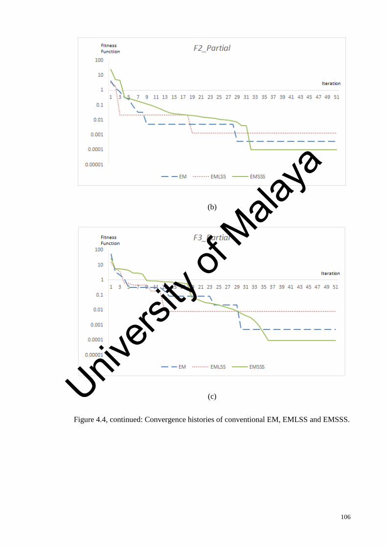
106

(b)

(c)

Figure 4.4, continued: Convergence histories of conventional EM, EMLSS and EMSSS.

Univers

ity of

Mala

ya

107

(d)

(e)

Figure 4.4, continued: Convergence histories of conventional EM, EMLSS and EMSSS.

Univers

ity of

Mala

ya

108

(f)

(g)

Figure 4.4, continued: Convergence histories of conventional EM, EMLSS and EMSSS.

Univers

ity of

Mala

ya

109

(h)

(i)

Figure 4.4, continued: Convergence histories of conventional EM, EMLSS and EMSSS.

Univers

ity of

Mala

ya

110

(j)

Figure 4.4, continued: Convergence histories of conventional EM, EMLSS and EMSSS.

4.1.4 Particles Movement Analysis

In order to better expose the movement of the particles during the convergence

process, the EMLSS and EMSSS were tested to solve the bowl-shaped Sphere test

function. For the ease of movement analysis, the dimension number of the test function

was set to 2. Table 4.4 shows the results of the best particles in a search for the minima

point performed by EMLSS.

Univers

ity of

Mala

ya

111

Table 4.4: Performance of EMLSS.

Ite Best Particle X Best Particle Y Best Particle fBest Particle

0 Particle 7 0.26 -1.66 2.8232

1 Particle 7 0.26 -0.67 0.5165

2 Particle 7 0.26 0.32 0.17

3 Particle 2 0.094943093 0.078857467 0.015232691

4 Particle 5 0.054285117 0.101797292 0.013309563

. . . . .

. . . . .

. . . . .

17 Particle 5 0.054285117 0.101797292 0.013309563

18 Particle 3 -0.024974939 0.049636075 0.003087488

. . . . .

. . . . .

. . . . .

100 Particle 3 -0.024974939 0.049636075 0.003087488

As shown in Table 4.4, particle number 7 had the initialized random values of

0.26 and -1.66 for X and Y respectively. This yielded an objective value of 2.8232, which

was the best among all other particles in the initialization. Particle 7 then searched locally

and achieved better result of 0.5165 in the first iteration and further improved it to 0.17

in the second iteration. Upon completing the third iteration, particle number 2 found a

better result, thus replaced particle number 7 to be the best particle in the iteration. In

iteration 4, particle 5 found an even better objective value at X= 0.054285117 and Y =

0.101797292. It maintained its position as the best particle until iteration 17. The search

reached its best minima point at the end of iteration 18, when particle number 3 found a

new best minima of 0.003087488 at X= -0.024974939 and Y = 0.049636075. The result

for the best particle remained the same from iteration 18 onwards to iteration 80.

Figure 4.5 shows the movement of the best particles from initialization (i0) to

iteration 18 (i18). All the different positions of the particles yielded different objective

values, as shown on the right side of the graph. The best particles moved from iteration

to iteration towards the origin point (0,0), where the best minima is located.

Univers

ity of

Mala

ya

112

Figure 4.5: Movement of best particles in EMLSS from iteration to iteration.

EMSSS, on the other hand, performed a much detailed search. Table 4.5 shows

the search history of the experiment. Since the search steps in EMSSS were comparatively

smaller, it caused the improvement in objective values to be relatively smaller as well. A

plot of graph in Figure 4.6 gives a better image on how the search mechanism was carried

out with a sample movement from iteration 8 to iteration 37 by particle 6, which was the

best particle in those iterations as it found the lowermost value in the minimization test

function. Particle 4 took over when it found a better objective value in iteration 38. The

movement scale of the plot shows smaller search steps compared to the movements in

BSL.

Univers

ity of

Mala

ya

113

Table 4.5. Performance of EMSSS.

Ite Best Particle X Best Particle Y Best Particle f Best Particle

0 Particle 7 0.97 -0.75 1.5034

1 Particle 7 0.96 -0.74 1.4692

2 Particle 7 0.95 -0.73 1.4354

3 Particle 6 -0.521062359 -0.667410792 0.716943148

4 Particle 6 -0.511062359 -0.657410792 0.693373685

5 Particle 9 -0.225239608 -0.629136921 0.446546146

6 Particle 9 -0.215239608 -0.619136921 0.429658615

7 Particle 9 -0.205239608 -0.609136921 0.413171085

8 Particle 6 -0.249784768 0.096136126 0.071634585

9 Particle 6 -0.239784768 0.086136126 0.064916167

10 Particle 6 -0.229784768 0.076136126 0.058597749

11 Particle 6 -0.229784768 0.066136126 0.057175027

12 Particle 6 -0.219784768 0.056136126 0.051456609

13 Particle 6 -0.209784768 0.046136126 0.046138191

14 Particle 6 -0.199784768 0.036136126 0.041219773

15 Particle 6 -0.189784768 0.026136126 0.036701355

16 Particle 6 -0.179784768 0.016136126 0.032582937

17 Particle 6 -0.169784768 0.006136126 0.028864519

18 Particle 6 -0.159784768 -0.003863874 0.025546101

19 Particle 6 -0.149784768 -0.003863874 0.022450406

20 Particle 6 -0.139784768 -0.003863874 0.019554711

21 Particle 6 -0.129784768 -0.003863874 0.016859015

22 Particle 6 -0.119784768 -0.003863874 0.01436332

23 Particle 6 -0.119784768 -0.003863874 0.01436332

24 Particle 6 -0.109784768 -0.003863874 0.012067625

25 Particle 6 -0.099784768 -0.003863874 0.009971929

26 Particle 6 -0.089784768 -0.003863874 0.008076234

27 Particle 6 -0.079784768 -0.003863874 0.006380539

28 Particle 6 -0.069784768 -0.003863874 0.004884843

29 Particle 6 -0.059784768 -0.003863874 0.003589148

30 Particle 6 -0.049784768 -0.003863874 0.002493453

31 Particle 6 -0.039784768 -0.003863874 0.001597757

32 Particle 6 -0.029784768 -0.003863874 0.000902062

33 Particle 6 -0.019784768 -0.003863874 0.000406367

34 Particle 6 -0.009784768 -0.003863874 0.000110671

35 Particle 6 0.000215232 -0.003863874 1.50E-05

36 Particle 6 0.000215232 -0.003863874 1.50E-05

37 Particle 6 0.000215232 -0.003863874 1.50E-05

38 Particle 4 0.001504167 -0.001954916 6.08E-06

. . . . .

. . . . .

. . . . .

100 Particle 4 0.001504167 -0.001954916 6.08E-06

Univers

ity of

Mala

ya

114

Figure 4.6: EMSSS local search movement by particle 6.

The solutions with highest accuracies are highlighted in boldface. The results

show EM with larger search steps reached near-optimal values faster with less iteration

number needed. The trade-off, however, is that the solutions returned by EMLSS are

generally less accurate compared to all the other EM algorithms. The large steps may skip

some of the better solutions between the steps, resulting in outcomes with lower

accuracies. EM with smaller search steps, on the other hand, returned outcomes which

are more accurate compared to EMLSS. Its small search steps enabled it to better exploit

the solutions, granting the algorithm to achieve final results with consistently higher

accuracies. However, the small steps employed requires more iterations to complete the

convergence, which in turn slow down the overall convergence process.

Univers

ity of

Mala

ya

115

4.2 SPC-EM

The proposed SPC-EM was tested in the designed test suite to analyse its

performance in solving numerical optimization problems. The results are compared with

that of the conventional EM, EMLSS and EMSSS. From the literature, Genetic Algorithm

(GA) is found to be one of the most established and well-known meta-heuristic algorithms.

Therefore, it is also included in the results benchmarking in order to effectively justify

the performance of the proposed algorithm. 20 independent runs were adopted in SPC-

EM to avoid stochastic discrepancy.

4.2.1 Performance Benchmarking

The comparisons of the computational results are shown in Tables 4.6. In each

table, “Best” indicates the best value ever obtained by the algorithm in the corresponding

test function throughout the 20 independent runs. “Mean” refers to the mean value of the

20 results obtained from the independent runs in solving the corresponding benchmark

function. “SD” denotes the respective standard deviation value of the results. “Rank”

stands for the performance comparison ranking of the search algorithm based on the mean

results (“Mean”).

Univers

ity of

Mala

ya

116

Table 4.6: Best values, worst values, mean values and standard deviations comparison

SPC-EM EM EMLSS EMSSS GA

F1 Best 1.4193E-03 3.5488E-03 4.5921E-02 3.8573E-03 3.0947E-02

Worst 1.4353E-03 2.7525E-01 4.1649E-01 1.2121E-02 2.6375E+00

Mean 1.4247E-03 1.0603E-01 2.0480E-01 7.6152E-03 5.9336E-01

SD 2.3926E-11 5.6446E-03 1.5163E-02 5.4233E-06 5.6891E-01

Rank 1 3 4 2 5

F2 Best 3.9364E-07 3.9145E-05 2.5787E-04 9.5861E-07 1.5779E-06

Worst 3.2743E-05 4.9154E-03 3.7381E-03 4.6775E-04 8.5408E-02

Mean 4.6110E-06 1.7701E-03 1.3424E-03 1.6460E-04 1.3026E-02

SD 6.1325E-11 2.5603E-06 7.9994E-07 2.5631E-08 5.5266E-04

Rank 1 4 3 2 5

F3 Best 1.2472E-06 1.4551E-05 5.4168E-04 5.3497E-05 1.7997E-05

Worst 2.0052E-06 9.7606E-03 9.3487E-03 5.2585E-04 2.2922E-02

Mean 1.3958E-06 3.5775E-03 5.1289E-03 1.5220E-04 1.2109E-02

SD 5.9082E-14 1.0620E-05 6.8173E-06 1.2121E-08 9.4126E-05

Rank 1 3 4 2 5

F4 Best 2.4944E-07 7.9371E-06 1.2766E-04 2.8497E-06 4.0000E-06

Worst 2.4997E-07 1.2945E-03 3.3039E-03 2.1470E-05 9.0000E-04

Mean 2.4962E-07 3.7616E-04 9.0476E-04 1.0529E-05 2.6330E-04

SD 2.8795E-20 1.3192E-07 6.0240E-07 3.5227E-11 5.4418E-08

Rank 1 4 5 2 3

F5 Best 3.6616E-06 1.5761E-05 1.7194E-04 1.1683E-05 3.2809E-05

Worst 5.8058E-06 9.1845E-03 9.5083E-03 4.6511E-04 4.5956E-02

Mean 3.8741E-06 3.3685E-03 4.3701E-03 1.9505E-04 7.9481E-03

SD 2.1121E-13 8.8754E-06 9.1427E-06 1.8427E-08 1.4531E-04

Rank 1 3 4 2 5

F6 Best 4.9526E-05 1.4493E-04 1.8655E-03 6.0471E-05 1.9855E-04

Worst 5.7421E-05 3.0677E-02 4.9664E-02 9.7521E-04 1.9884E+00

Mean 5.1338E-05 1.1116E-02 1.9877E-02 5.1123E-04 2.6310E-01

SD 5.6796E-12 9.6784E-05 2.2039E-04 7.4025E-08 2.7924E-01

Rank 1 3 4 2 5

F7 Best 2.4945E-05 4.8441E-05 9.8546E-04 4.1846E-05 1.4607E-04

Worst 2.8149E-05 2.8021E-02 3.9921E-02 1.2764E-03 9.0797E-02

Mean 2.5914E-05 8.4205E-03 1.4243E-02 4.7670E-04 3.3102E-02

SD 8.6973E-13 5.4449E-05 1.3299E-04 1.6155E-07 9.1038E-04

Rank 1 3 4 2 5

F8 Best 1.1102E-16 4.4633E-12 1.5314E-07 6.4951E-11 1.1000E-07

Worst 2.0630E-05 3.0381E-05 2.3740E-05 7.1495E-06 7.1922E-04

Mean 1.4542E-06 3.3250E-06 4.5667E-06 1.8545E-06 1.8244E-04

SD 2.0079E-11 4.6258E-11 4.5498E-11 6.1744E-12 4.7147E-08

Rank 1 3 4 2 5

F9 Best -186.7304 -186.7259 -186.7010 -186.7300 -186.7299

Worst -186.7303 -186.5277 -186.3577 -186.6749 -169.5802

Mean -186.7303 -186.6603 -186.5090 -186.7030 -185.3659

SD 5.4656E-10 3.4926E-03 9.7112E-03 2.7069E-04 1.3925E+01

Rank 1 3 4 2 5

F10 Best -1.03162780 -1.03162337 -1.03159788 -1.03162720 -1.03162500

Worst -1.03162745 -1.03011631 -1.03007554 -1.03152877 -1.02697000

Mean -1.03162749 -1.03101462 -1.03104713 -1.03157383 -1.03044870

SD 5.2578E-15 2.2573E-07 1.2621E-07 6.3617E-10 1.1913E-06

Rank 1 4 3 2 5

Univers

ity of

Mala

ya

117

The benchmarking reveals the striking capability of SPC-EM in obtaining optimal

solutions with higher accuracy and precision. The solutions found by SPC-EM are

relatively much better than the solutions found by the conventional EM, EMLSS, EMSSS,

and GA. The systematically-self-regulating probe length feature of the SPC-EM enabled

it to effectively exploit the solutions. The fine-tuned search steps towards the end of the

local search every time also ensured the precision of the algorithm, which in turn resulted

in lower standard deviation values as shown in the table. From the overall analysis on the

results benchmarking, SPC-EM outperformed all the other algorithms involved.

4.2.2 Convergence Process Analysis

Figures 4.7 show the convergence curves of the benchmarked algorithms in all the

test functions. The graphs are focused on the first 50 iterations of the convergences where

most of the movements took place. Logarithmic axis is not applicable in test functions F9

and F10 due to the negative values of the objective functions. It can be noted from the

graphs that the SPC-EM performed well in solving variable types of complex

optimization problems in terms of the accuracy of the solutions and overall convergence

performance. The SPC-EM progressed very rapidly in early stages and found near-

optimal values in relatively earlier iterations in most of the cases. The ability for the SPC-

EM to reach near optimum values in earlier stage of convergence was due to its long

probe lengths at the beginning of the search. The regulated and fine-tuned probe lengths

towards the end of the local search of SPC-EM enabled it to achieve solutions with

relatively higher accuracy. The tuning of the probe lengths helped SPC-EM to outperform

other algorithms in their overall convergence process.

Univers

ity of

Mala

ya

118

(a)

(b)

Figure 4.7: Convergence histories comparison of SPC-EM, conventional EM, EMLSS,

EMSSS and GA.

Univers

ity of

Mala

ya

119

(c)

(d)

Figure 4.7, continued: Convergence histories comparison of SPC-EM, conventional

EM, EMLSS, EMSSS and GA.

Univers

ity of

Mala

ya

120

(e)

(f)

Figure 4.7, continued: Convergence histories comparison of SPC-EM, conventional

EM, EMLSS, EMSSS and GA.

Univers

ity of

Mala

ya

121

(g)

(h)

Figure 4.7, continued: Convergence histories comparison of SPC-EM, conventional

EM, EMLSS, EMSSS and GA.

Univers

ity of

Mala

ya

122

(i)

(j)

Figure 4.7, continued: Convergence histories comparison of SPC-EM, conventional

EM, EMLSS, EMSSS and GA.

Univers

ity of

Mala

ya

123

4.3 ELEM

The same experiment setup was used to test the proposed ELEM. The experiment

for each of the tests were carried out 20 times to avoid stochastic discrepancy. The results

obtained by ELEM are compared with the conventional EM, EMLSS, EMSSS and GA

in terms of the best solutions, worst solutions, mean values and standard deviations of the

20 independent runs.

4.3.1 Performance Benchmarking

Table 4.7 shows the results comparison of ELEM with other algorithms in terms

of the best solutions, worst solutions, mean values, and standard deviations of the 20

independent runs. Based on the mean values, ELEM ranks the first place compared to

other algorithms. The overall result comparisons reveal the potential of ELEM in

achieving optimal solutions with higher accuracies and precisions. ELEM steadily shows

better performance in contrast with the conventional EM, EMLSS, EMSSS and GA.

EMSSS shows very competitive results on the best solutions achieved in test functions

F2, F6, F7, and F9. It even outperforms ELEM in the worst value achieved column in F8.

ELEM shows very promising performance in solving multi-model functions, such as F1,

F5, F6, F8, F9, and F10. The strong exploration ability of EM paired with the powerful

experience-based exploitation mechanism enabled ELEM to escape local traps and

returns with high accuracy solutions.

Univers

ity of

Mala

ya

124

Table 4.7: Comparison on the best solutions, worst solutions, mean values, and standard

deviations generated by ELEM with the other benchmark algorithms.

ELEM EM EMLSS EMSSS GA

F1 Best 2.3785E-04 3.5488E-03 4.5921E-02 3.8573E-03 3.0947E-02

Worst 9.6410E-04 2.7525E-01 4.1649E-01 1.2121E-02 2.6375E+00

Mean 8.0935E-04 1.0603E-01 2.0480E-01 7.6152E-03 5.9336E-01

SD 6.6424E-08 5.6446E-03 1.5163E-02 5.4233E-06 5.6891E-01

Rank 1 3 4 2 5

F2 Best 1.7511E-07 3.9145E-05 2.5787E-04 9.5861E-07 1.5779E-06

Worst 1.6450E-05 4.9154E-03 3.7381E-03 4.6775E-04 8.5408E-02

Mean 3.0747E-06 1.7701E-03 1.3424E-03 1.6460E-04 1.3026E-02

SD 1.8329E-11 2.5603E-06 7.9994E-07 2.5631E-08 5.5266E-04

Rank 1 4 3 2 5

F3 Best 5.5609E-07 1.4551E-05 5.4168E-04 5.3497E-05 1.7997E-05

Worst 1.3053E-06 9.7606E-03 9.3487E-03 5.2585E-04 2.2922E-02

Mean 7.6655E-07 3.5775E-03 5.1289E-03 1.5220E-04 1.2109E-02

SD 9.9573E-14 1.0620E-05 6.8173E-06 1.2121E-08 9.4126E-05

Rank 1 3 4 2 5

F4 Best 1.1096E-07 7.9371E-06 1.2766E-04 2.8497E-06 4.0000E-06

Worst 1.1162E-07 1.2945E-03 3.3039E-03 2.1470E-05 9.0000E-04

Mean 1.1106E-07 3.7616E-04 9.0476E-04 1.0529E-05 2.6330E-04

SD 2.1177E-20 1.3192E-07 6.0240E-07 3.5227E-11 5.4418E-08

Rank 1 4 5 2 3

F5 Best 1.6275E-06 1.5761E-05 1.7194E-04 1.1683E-05 3.2809E-05

Worst 3.5498E-06 9.1845E-03 9.5083E-03 4.6511E-04 4.5956E-02

Mean 1.9761E-06 3.3685E-03 4.3701E-03 1.9505E-04 7.9481E-03

SD 3.2895E-13 8.8754E-06 9.1427E-06 1.8427E-08 1.4531E-04

Rank 1 3 4 2 5

F6 Best 2.2032E-05 1.4493E-04 1.8655E-03 6.0471E-05 1.9855E-04

Worst 2.2343E-05 3.0677E-02 4.9664E-02 9.7521E-04 1.9884E+00

Mean 2.2060E-05 1.1116E-02 1.9877E-02 5.1123E-04 2.6310E-01

SD 4.6304E-15 9.6784E-05 2.2039E-04 7.4025E-08 2.7924E-01

Rank 1 3 4 2 5

F7 Best 1.1120E-05 4.8441E-05 9.8546E-04 4.1846E-05 1.4607E-04

Worst 2.7677E-05 2.8021E-02 3.9921E-02 1.2764E-03 9.0797E-02

Mean 1.3260E-05 8.4205E-03 1.4243E-02 4.7670E-04 3.3102E-02

SD 1.5737E-11 5.4449E-05 1.3299E-04 1.6155E-07 9.1038E-04

Rank 1 3 4 2 5

F8 Best 0.0000E+00 4.4633E-12 1.5314E-07 6.4951E-11 1.1000E-07

Worst 7.5275E-06 3.0381E-05 2.3740E-05 7.1495E-06 7.1922E-04

Mean 4.2922E-07 3.3250E-06 4.5667E-06 1.8545E-06 1.8244E-04

SD 2.6611E-12 4.6258E-11 4.5498E-11 6.1744E-12 4.7147E-08

Rank 1 3 4 2 5

F9 Best -186.7307 -186.7259 -186.7010 -186.7300 -186.7299

Worst -186.7304 -186.5277 -186.3577 -186.6749 -169.5802

Mean -186.7306 -186.6603 -186.5090 -186.7030 -185.3659

SD 5.4818E-09 3.4926E-03 9.7112E-03 2.7069E-04 1.3925E+01

Rank 1 3 4 2 5

F10 Best -1.03162802 -1.03162337 -1.03159788 -1.03162720 -1.03162500

Worst -1.03162792 -1.03011631 -1.03007554 -1.03152877 -1.02697000

Mean -1.03162801 -1.03101462 -1.03104713 -1.03157383 -1.03044870

SD 4.9932E-16 2.2573E-07 1.2621E-07 6.3617E-10 1.1913E-06

Rank 1 4 3 2 5

Univers

ity of

Mala

ya

125

4.3.2 Convergence Process Analysis

Figures 4.8 graphically present the comparison on typical convergence

characteristics between the ELEM, GA, and the variants of EM involved in the

benchmarking. It can be clearly observed from the graphs that the ELEM performed well

in different complex optimization problems both in terms of the quality of the solution

and convergence speed. The gradient analysis of the ELEM and its ability to backtrack

the experience of previous searches enable it to perform a well-directed local search. This

advantage was balanced by a well-diversified solutions search in the global movement

stage of the ELEM, where the particles were moved in accordance to the attraction and

repulsion forces influenced by all other particles in the search space. With the

combination of the two advantages, the ELEM algorithm converged more rapidly and

reached lower objective values than other algorithms, Lower objective values indicate

solutions with higher accuracies.

(a)

Figure 4.8, continued: Convergence history comparison of ELEM and other algorithms.

Univers

ity of

Mala

ya

126

(b)

(c)

Figure 4.8, continued: Convergence history comparison of ELEM and other algorithms.

Univers

ity of

Mala

ya

127

(d)

(e)

Figure 4.8, continued: Convergence history comparison of ELEM and other algorithms.

Univers

ity of

Mala

ya

128

(f)

(g)

Figure 4.8, continued: Convergence history comparison of ELEM and other algorithms.

Univers

ity of

Mala

ya

129

(h)

(i)

Figure 4.8, continued: Convergence history comparison of ELEM and other algorithms.

Univers

ity of

Mala

ya

130

(j)

Figure 4.8, continued: Convergence history comparison of ELEM and other algorithms.

4.3.3 Parameter Sensitivity Test

In this section, the effect of α and β settings on the performance of the ELEM

algorithm is investigated. Simulations were carried out where the algorithm was executed

independently 20 times on each benchmark test function with different settings of α and

β. The value of the gain factor, α was limited to vary from 1.1 to 1.5 as it was estimated

that a gain too large can generate an out-of-proportion λ size. For similar reason, the value

of the penalty factor, β was limited to vary from 0.5 to 0.9. The mean results generated

by pairing increasing α with increasing β values are summarized in Tables 4.8, while

Table 4.9 shows the outcomes obtained by pairing increasing α with decreasing β. The

best solutions are highlighted in boldface.

Univers

ity of

Mala

ya

131

Table 4.8: Results generated by pairing increasing α with increasing β.

α=1.1

β=0.5

α=1.2

β=0.6

α=1.3

β=0.7

α=1.4

β=0.8

α=1.5

β=0.9

F1 1.8842E-02 3.7731E-03 3.1124E-03 6.4779E-02 3.7888E-02

F2 9.6901E-05 4.9592E-06 9.1646E-05 3.1034E-03 6.3541E-04

F3 9.1630E-04 3.1846E-06 4.1956E-06 3.7929E-05 2.4648E-05

F4 3.0848E-06 9.1750E-07 3.8827E-05 6.5751E-06 6.4104E-04

F5 5.0405E-03 6.5901E-06 3.0366E-05 3.4126E-03 3.1622E-03

F6 3.1954E-02 3.2260E-03 7.9021E-05 3.1645E-02 3.0305E-04

F7 2.9763E-04 7.9311E-04 2.9006E-03 6.1552E-03 2.5645E-04

F8 6.0772E-03 6.3091E-02 1.0979E-05 3.3923E-07 6.8741E-05

F9 -186.730133 -186.730528 -186.730471 -186.730241 -186.730586

F10 -1.03161688 -1.03162762 -1.03162675 -1.03162432 -1.03162181

Table 4.9: Results generated by pairing increasing α with decreasing β.

α=1.1

β=0.9 α=1.2

β=0.8

α=1.3

β=0.7

α=1.4

β=0.6

α=1.5

β=0.5

F1 6.4644E-03 9.3732E-04 3.1124E-03 9.1788E-02 3.9511E-02

F2 7.1195E-06 3.3910E-06 9.1646E-05 6.1263E-04 6.8411E-05

F3 9.1264E-06 7.4061E-07 4.1956E-06 8.0242E-03 3.7962E-04

F4 6.2338E-06 2.5348E-07 3.8827E-05 3.7121E-06 4.3860E-05

F5 3.4004E-06 3.1928E-06 3.0366E-05 5.0906E-05 2.8377E-04

F6 9.8919E-05 7.2856E-05 7.9021E-05 3.1665E-03 6.1720E-03

F7 6.4407E-04 8.1555E-05 2.9006E-03 3.8337E-02 3.0028E-02

F8 6.3160E-08 9.1616E-07 1.0979E-05 6.0028E-03 6.4552E-05

F9 -186.730422 -186.730601 -186.730471 -186.729702 -186.729288

F10 -1.03162771 -1.03162800 -1.03162675 -1.03162391 -1.03162442

The results in Table 4.8 and 4.9 indicate that the setting of parameters α and β

shows certain impact on the performance of the ELEM. It can be observed from the tables

that for most benchmark functions, the ELEM showed the best performance when the

gain factor, α was set to 1.2 and the penalty factor, β was set to 0.8. When α was set to

1.0, it began to show under gain while any value over 1.2 showed over gain on the step

tuning. Over gain led to an oversized search step in the local search procedure, causing it

to overstep any better solution within the step. Under gain, on the other hand, caused the

search to reach the best solution in relatively later iterations. Similar situations can also

be observed for the setting of parameter β, where 0.9 showed over compensation, while

Univers

ity of

Mala

ya

132

values under 0.8 caused under compensation. As a whole, ELEM with α = 1.2 and β =

0.8 shows the best performance among the tested algorithms.

4.3.4 ELEM vs SPC-EM

The SPC-EM and the ELEM both proved improvements compared to the

conventional EM. In this section, the performance of the experience-based ELEM is

compared with the iteration-based step regulation SPC-EM. Table 4.10 shows the

comparison of the results obtained by the ELEM and the SPC-EM. From the table, it can

be observed that the ELEM outperformed the SPC-EM in all of the test functions. The

SPC-EM shows very competitive solutions in many of the tests, such as F2, F3, F4, F5,

F6, F7, and F9. However in the end, the ELEM proved to be superior in term of solution

accuracies.

Univers

ity of

Mala

ya

133

Table 4.10: Results comparison of ELEM vs SPC-EM.

ELEM SPC-EM

F1 Best 2.3785E-04 1.4193E-03

Worst 9.6410E-04 1.4353E-03

Mean 8.0935E-04 1.4247E-03

SD 6.6424E-08 2.3926E-11

Rank 1 2

F2 Best 1.7511E-07 3.9364E-07

Worst 1.6450E-05 3.2743E-05

Mean 3.0747E-06 4.6110E-06

SD 1.8329E-11 6.1325E-11

Rank 1 2

F3 Best 5.5609E-07 1.2472E-06

Worst 1.3053E-06 2.0052E-06

Mean 7.6655E-07 1.3958E-06

SD 9.9573E-14 5.9082E-14

Rank 1 2

F4 Best 1.1096E-07 2.4944E-07

Worst 1.1162E-07 2.4997E-07

Mean 1.1106E-07 2.4962E-07

SD 2.1177E-20 2.8795E-20

Rank 1 2

F5 Best 1.6275E-06 3.6616E-06

Worst 3.5498E-06 5.8058E-06

Mean 1.9761E-06 3.8741E-06

SD 3.2895E-13 2.1121E-13

Rank 1 2

F6 Best 2.2032E-05 4.9526E-05

Worst 2.2343E-05 5.7421E-05

Mean 2.2060E-05 5.1338E-05

SD 4.6304E-15 5.6796E-12

Rank 1 2

F7 Best 1.1120E-05 2.4945E-05

Worst 2.7677E-05 2.8149E-05

Mean 1.3260E-05 2.5914E-05

SD 1.5737E-11 8.6973E-13

Rank 1 2

F8 Best 0.0000E+00 1.1102E-16

Worst 7.5275E-06 2.0630E-05

Mean 4.2922E-07 1.4542E-06

SD 2.6611E-12 2.0079E-11

Rank 1 2

F9 Best -186.7307 -186.7304

Worst -186.7304 -186.7303

Mean -186.7306 -186.7303

SD 5.4818E-09 5.4656E-10

Rank 1 2

F10 Best -1.03162802 -1.03162780

Worst -1.03162792 -1.03162745

Mean -1.03162801 -1.03162749

SD 4.9932E-16 5.2578E-15

Rank 1 2

Univers

ity of

Mala

ya

134

The sampled convergence processes of the ELEM are also compared with that of

the SPC-EM in Figure 4.9. Since it is not feasible to show F9 and F10 in algorithmic axis,

the graphs are shown without taking the initialization iteration values as the scales of the

movements after the initialization stage are relatively too small to be visible. The ELEM

achieves comparatively lower solution values in most of the sampled convergence, except

for F8. Given the nature of the graph shape in Schaffer N2 test, the sharp spikes pose

many local optima traps, rendering differential type local search mechanism to show

limitations. In problems as such, the exploration ability of the algorithm plays a more

important role in diversifying the search for other optima points. In term of convergence

rate, it can be observed from the all the comparisons that both algorithms are equally rapid

in most of the test functions. In some of the tests, such as F3 and F6, ELEM shows slightly

quicker convergence.

(a)

Figure 4.9: Convergence rate comparisons of ELEM vs SPC-EM.

Univers

ity of

Mala

ya

135

(b)

(c)

Figure 4.9, continued: Convergence rate comparisons of ELEM vs SPC-EM.

Univers

ity of

Mala

ya

136

(d)

(e)

Figure 4.9, continued: Convergence rate comparisons of ELEM vs SPC-EM.

Univers

ity of

Mala

ya

137

(f)

(g)

Figure 4.9, continued: Convergence rate comparisons of ELEM vs SPC-EM.

Univers

ity of

Mala

ya

138

(h)

(i)

Figure 4.9, continued: Convergence rate comparisons of ELEM vs SPC-EM.

Univers

ity of

Mala

ya

139

(j)

Figure 4.9, continued: Convergence rate comparisons of ELEM vs SPC-EM.

4.4 EM in MPPT

To test the performance of the enhanced EM in solving engineering optimization

problems, the proposed ELEM was implemented in the simulation to track the MPP of a

PV solar harvesting system. First, ELEM was tested to track the MPP of 3 serial-

connected BP Solar MSX-120W PV panels under ideal and uniform irradiance. As

mentioned in Chapter 3, the Power-Voltage behaviour of the simulated PV array under

ideal and uniform irradiance is as shown in Figure 4.10.

Univers

ity of

Mala

ya

140

Figure 4.10: P-V curve of the serial-connected arrays under ideal irradiance.

4.4.1 Ideal Irradiance

Simulations were carried out 20 times and some results were sampled and

analysed. Figure 4.11 shows an example of the convergence of the ELEM in the MPPT

simulation under uniform insolation. The modified ELEM was quick in locating the MPP

as the single peak P-V characteristic of the PV array under uniform irradiance required

relatively easier convergence process. Univers

ity of

Mala

ya

141

Figure 4.11: MPPT convergence of the ELEM under ideal irradiance.

Table 4.11 shows an example of the particle movement in search of the MPP under

the enhanced exploitation procedure proposed in the ELEM. Figure 4.12 gives a better

illustration of the movements in the form of a Power vs Voltage graph. It can be observed

from Figure 4.12 that the best particle began the search procedure in the initial position

marked in the graph. It then moved in search for a higher power point towards the peak

of the P-V curve (refer Figure 4.11) until it finally hit the MPP of 360W at 33.7V. Figure

4.13 shows the sampled local search convergence process.

Table 4.11: Example of local search particle displacement of the ELEM in tracking the

MPP.

Ite Voltage (V) Power (W)

0 30.08889 324.9600

1 30.97778 334.5600

2 31.86667 344.1600

3 32.75556 355.4492

4 33.64444 359.9844

5 33.70000 360.0000

6 33.70000 360.0000

7 33.70000 360.0000

- - -

- - -

- - -

Univers

ity of

Mala

ya

142

Figure 4.12: Particle movement in search for the MPP under ideal irradiance condition.

Figure 4.13: The exploitation progress in search of the MPP under ideal irradiance

condition.

Univers

ity of

Mala

ya

143

4.4.2 Partial Shaded Condition

In practical applications, the solar irradiance onto the PV arrays is seldom uniform.

Shadows of clouds, buildings and accumulated dust can disturb the insolation of the PV

arrays, causing non-uniform irradiance to the PV arrays (Boukenoui, 2016). The rapidly

changing shading pattern makes it even harder for the PV system to perform effectively.

To simulate challenging partial shading conditions as such, the algorithm was tested to

track for the MPP under 3 changing shading patterns, as shown in Figure 4.14. In the

simulation, the P-V curve of the shading pattern was as shown in Figure 4.14 (a) during

the first second. Then, in the following second, the P-V curve changed into Pattern 2,

representing changes in the shading pattern on the PV array. In the third second, the

shading pattern changed again into pattern 3 with the P-V curve as shown in Figure 4.14

(c).

Figure 4.14 (a): Simulated pattern 1 of shading condition.

Univers

ity of

Mala

ya

144

Figure 4.14 (b): Simulated pattern 2 of shading condition.

Figure 4.14 (c): Simulated pattern 3 of shading condition.

Univers

ity of

Mala

ya

145

Simulations were carried out 20 times and some results were sampled and

analysed. Figure 4.15 shows an example of the result obtained by implementing ELEM

in the MPPT of the PV system under varying shading condition. It can be observed that

the algorithm successfully found the MPP under the first shading pattern (MPP1). The

operating voltage remained at 21.86V until the shading condition changed to the second

shading pattern. The algorithm carefully tracked the MPP as it dropped to MPP2 at

102.852W. When the shading pattern changed again to pattern 3, the algorithm followed

and tracked the MPP to 253.32W. It can be concluded from this observation that the

ELEM successfully tracked the MPP as it moved under different PSC patterns.

Figure 4.15: The MPPT successfully performed by ELEM under changing PSCs from

pattern 1 to pattern 2 and then to pattern 3.

Figure 4.16 (a), (b), and (c) show some sampled movements of the particles in

tracking the MPPs under shading pattern 1, 2, and 3 respectively. These movements gives

a clear picture on how the algorithm tracks the MPP by adjusting the Voltage.

Univers

ity of

Mala

ya

146

Figure 4.16: Particle movement in search of the MPPs in PSC pattern 1, pattern 2 and

pattern 3.

Literature study shows that the P&O is one of the most commonly applied

algorithms in the MPPT of a PV system. Thus, the performance of the ELEM is also

compared with a conventional P&O with random perturbation length setting. Simulations

with P&O were also carried out 20 times. Result was sampled and shown in Figure 4.17.

It can be observed that in this example that in shading pattern 1 and 3, P&O was trapped

in the local optima for some time before managed to escape them. It is important for an

MPPT algorithm to avoid local MPP traps as they can cause unnecessary loss of energy.

Univers

ity of

Mala

ya

147

Figure 4.17. Performance comparison of ELEM vs P&O.

In the case of a PV solar energy harvesting system, the main challenge of the

MPPT mechanism is to adjust the output Voltage in order to optimize the output power

under different irradiance conditions. The simulation results in this section indicate that

ELEM is successful in tracking the maximum power point of a PV solar harvesting

system under uniform irradiance, non-uniform irradiance, and varying shading conditions.

Univers

ity of

Mala

ya

148

CHAPTER 5: CONCLUSION

The Electromagnetism-like Mechanism algorithm is a population based meta-

heuristic search method. Mimicking the attraction and repulsion mechanisms in the

electromagnetism theorem, the EM is designed to search for the global optimum point in

a continuous search space. In this research, extensive studies have been carried out to

learn the behaviour of this algorithm. Modifications and improvements are proposed to

further enhance the performance of it. The enhanced EM is then tested to solve

engineering optimization problem.

The effect of the search step size setting on the convergence performance of the

EM was investigated by modifying a conventional EM to search in two different extreme

sets of step size settings. EMLSS was set to search in relatively larger steps, while EMSSS

conducted the search in smaller search step setting. Experimental results showed that

larger and smaller search step size settings both have their respective advantages and

disadvantages. Larger step settings speeded up the convergence process, but the final

results returned by the algorithm is comparatively less accurate. Smaller step settings, on

the other hand, yielded results with higher accuracies. The trade off, however, was that

the algorithm required significantly more iterations before it obtained the final outcome,

which in turn rendered the overall convergence process to be slower.

In order to acquire the advantages from both large and small search step settings,

a local search scheme with a dynamic tuning mechanism, known as the Split, Probe and

Univers

ity of

Mala

ya

149

Compare mechanism was developed for the EM in this research. The SPC mechanism is

a solution exploitation scheme created to replace the entire local search segment of a

conventional EM. This search scheme enhances the EM with the ability to hit a more

accurate solution without heavily slowing down the entire convergence process. The

search mechanism probes for better solutions in split directions in the dimension. A

nonlinear equation has been designed to systematically and dynamically adjust the length

of the probes based on the outcome of the Compare segment in each iteration. The general

concept of the tuning strategy is to begin the search with relatively longer probes and

dynamically tune the probe lengths as iterations go. Experiments on 10 different test

problems reveal that the modified algorithm performed well in solving numerical

optimization problems. The proposed modification onto the algorithm brought significant

improvements especially in term of solutions exploitation.

Besides SPC-EM, an experience-based search strategy has also been successfully

developed and introduced into the EM. The Experiential-Learning EM is enhanced with

the ability to learn from previous search experience and adjust the scale and direction of

the following search iterations. A trail memory was generated as iterations went on,

allowing the algorithm to remember and backtrack previous search results and

improvement rates. In addition, the ELEM employed a more directional search approach

instead of a random line search in a conventional EM. This approach significantly

improved the exploitation ability of the algorithm. Combining with the powerful

exploration mechanism of the EM, the proposed ELEM stroke a good balance in

searching for well diversified solutions and accurately exploited results. In the experiment

of 10 complex optimization problems, the ELEM showed significant superiority in terms

of solution accuracies and convergence efficiencies compared to all other algorithms

Univers

ity of

Mala

ya

150

involved in the benchmarking. The ELEM also proved to outperform the SPC-EM in the

same test suite.

The ELEM was implemented in the simulation to track the maximum power point

of a PV solar energy harvesting system. Experiment on a PV array with 3 serial-connected

PV panels was carried out. Simulations of changing shading patterns were carried out to

mimic the challenging shading conditions in the actual applications. The algorithm was

tested to track the moving MPP caused by the changing shading conditions. Results

showed that the enhanced EM was successful in tracking the MPP under uniform

irradiance, non-uniform irradiance, and rapid changing shading conditions with moving

MPPs. A maximum power point tracking scheme for a PV system adopting the

advantages of the ELEM has been successfully developed. The achievement of the ELEM

in this experiment also proved the capability of it in solving actual engineering

optimization problems.

As a conclusion, all the aims and objectives of this research are successfully

achieved. In the future, inter-particle experience sharing feature can be considered for the

betterment of the EM. Sharing local information with immediate neighbours can be very

helpful in speeding up the local search procedure. Furthermore, there is also possibility

to apply the experience-learning feature into the exploration segment of the EM to further

enhance the diversification of the solutions. The proposed SPC and Experiential Learning

features can also be introduced into other population-based global optimization

algorithms, such as particle swarm optimization, ant colony optimization, and artificial

bee colony in the future work. The ability to learn from previous experience can be very

useful in enhancing the convergence performance of these algorithms. It is also suggested

Univers

ity of

Mala

ya

151

that in time to come, the implementation of the ELEM can be extended to track the global

MPPs of other energy harvesting systems with multiple local peaks, as well as other

engineering optimization problems with the need of global optima searching.

Univers

ity of

Mala

ya

152

REFERENCES

Abdelsalam Ahmed K, Massoud Ahmed M, Shehab Ahmed, Enjeti Prasad N (2011).

High performance adaptive perturb and observe MPPT technique for

photovoltaic-based micro grids. IEEE Trans Power Electron, 26(4):1010–21.

Ahmed Jubaer, Salam Zainal (2015). An improved perturb and observe (P&O)

maximum power point tracking (MPPT) algorithm for higher efficiency. Appl

Energy, 150:97108.

Alabedin AMZ, El-Saadany EF, Salama MMA (2011). Maximum power point tracking

for photovoltaic systems using fuzzy logic and artificial neural networks. IEEE

Power Energy Soc Gen Meet, 1–9.

Alajmi BN, Ahmed KH, Finney SJ, Williams BW (2013). A maximum power point

tracking technique for partially shaded photovoltaic systems in microgrids. IEEE

Trans Ind Electron, 60:1596–606.

Al-Amoudi A, Zhang L (1998). Optimal control of a grid-connected PV system for

maximum power point tracking and unity power factor. In:Proceedings of the 7th

international conference on power electronics variable speed drives, p.80–85.

Al-Amoudi A, Zhang L (2000). Application of radial basis function networks for solar

array modelling and maximum power-point prediction. In:IEEE Proceedings of

the Generation, Transmission and Distribution, IET, p.310–6.

Ali Sharifi, Vahid Noroozi, Masoud Bashiri, Ali B. Hashemi, Mohammad Reza

Meybodi (2012). Two Phased Cellular PSO: A New Collaborative Cellular

Algorithm for Optimization in Dynamic Environments. WCCI 2012 IEEE

World Congress on Computational Intelligence, Brisbane, Australia.

Amrouche B, Guessoum A, Belhamel M (2012). A simple behavioural model for solar

module electric characteristics based on the first order system step response for

MPPT study and comparison. Appl Energy, 91:395–404.

Ansari F, Iqbal A, Chatterji S, Afzal A (2009). Control of MPPT for photovoltaic

systems using advanced algorithm EPP. In: Proceedings of international

conference on power systems ICPS, 1:6, p. 27-9.

Arcidiacono V, Corsi S, Lambri L (1982). Maximum power point tracker for

photovoltaic power plants. In: Proc IEEE photovoltaic spec conf, p. 507–12.

Armstrong S, Hurley WG (2010). A new methodology to optimize solar energy

extraction under cloudy conditions. Renewable Energy, 35:780–7.

Arora, J.S., Elwakeil, O.A., & Chahande, A.I. (1995). Global optimization methods for

engineering applications: a review. Structural Optimization, 9, 137-159.

Univers

ity of

Mala

ya

153

Ashiru I., Czanecki C., Routen T. (1995). Intelligent operators and optimal genetic-

based path planning for mobile robots, Proceedings of the International

Conference on Recent Advances in Mechatronics, Istanbul, Turkey, August, pp.

1018–1023.

Bagis Aytekin (2008). Fuzzy rule base design using tabu search algorithm for nonlinear

system modeling. ISA Trans, 47:32–44.

Bahgat A, Helwa N, Ahmad G, El Shenawy E (2005). Maximum power point tracking

controller for PV systems using neural networks. Renew Energy, 30:1257–68.

Bakirci K (2009). Models of solar radiation with hours of bright sunshine: a review.

Renewable and Sustainable Energy Reviews, 13:2580–8.

Barr A, Feigenbaum EA (1981). The handbook of artificial intelligence, vol. 1. Los

Altos, CA: Morgan Kaufmann.

Beasley D, Bull DR, Martin RR (1993). An overview of genetic algorithms:Part 1,

fundamentals. University Computing, 15(2):58–69.

Birbil S. I. and Fang S. C. (2003). “An electromagnetism-like mechanism for global

optimization,” Journal of Global Optimization, vol. 25, no.3, pp. 263-282.

Bodur M, Ermis M (1994). Maximum power point tracking for low power photovoltaic

solar panels. In: Proc 7th Mediterranean electrotechnical conf, p. 758–61.

Boukenoui R., Salhi H., Bradai R., Mellit A. (2016). A new intelligent MPPT method

for stand-alone photovoltaic systems operating under fast transient variations of

shading patterns. Solar Energy, 124:124–142.

Bratton D., Kennedy J. (2007). Defining a standard for particle swarm optimization,

Proceedings of the 2007 IEEE Swarm Intelligence Symposium, 120 - 127.

Burke EK, Kendall G (2005). Search methodologies: Introductory Tutorials in

Optimization and Decision Support Techniques. New York: Springer-Verlag.

Cacciato M, Consoli A, Attanasio R, Gennaro F (2010). Soft-switching converter with

HF transformer for grid-connected photovoltaic systems. IEEE Trans Ind

Electron, 57(5):1678–86.

Carrano EG, Guimarães FG, Takahashi RH, Neto OM, Campelo F (2007). Electric

distribution network expansion underload-evolution uncertainty using an

immune system inspired algorithm. IEEE Trans Power Sys,22:851–61.

Chandel SS, Aggarwal RK, Pandey AN (2005). New correlation to estimate global solar

radiation on horizontal surfaces using sunshine hour and temperature data for

Indian sites. Journal of Solar Energy Engineering, 127 (3):417–20.

Chang Y (2010). Optimal the tilt angles for photovoltaic modules using PSO method

with nonlinear time-varying evolution. Energy, 35:1954–63.

Univers

ity of

Mala

ya

154

Charniak E, McDermott D (1985). Introduction to artificial intelligence. Reading, MA:

Addison Wesley.

Chee Wei T, Green TC, Hernandez-Aramburo CA (2007). A current mode controlled

maximum power point tracking converter for building integrated photo- voltaics.

In: Proceedings of European conference on power electronics and applications.

Chelouah R, Siarry P (2005). A hybrid method combining continuous tabu search and

Nelder–Mead simplex algorithms for the global optimization of multi minima

functions. Eur.J.Oper.Res, 161:636–54.

Chen LR, Tsai CH, Lin YL, Lai YS (2010). A biological swarm chasing algorithm for

tracking the PV maximum power point. IEEE Trans Energy Convers, 25:484–93.

Chen YM, Lee CH, Wu HC (2005). Calculation of the optimum installation angle for

fixed solar-cell panels based on the genetic algorithm and the simulated

annealing method.IEEE Trans Energy Conversion, 20 (2):467–73.

Chen Z (2000). Computational intelligence for decision support. Boca Raton, FL: CRC

Press.

Chian-Song C (2010). T–S fuzzy maximum power point tracking control of solar power

generation systems. IEEE Trans Energy Convers, 25:1123–32.

Cho B.J., Hong S.C., Okoma S. (1996). Job shop scheduling using genetic algorithm,

Proceedings of the Third World Congress on Expert Systems, Seoul, Korea,

February, pp. 351–358.

Chowdhury SR, Saha H (2010). Maximum power point tracking of partially shaded

solar photovoltaic arrays. Sol Energy Mater Sol Cells, 94:1441–7.

Čongradac V, Prica M, Paspalj M, Bojanič D, Čapko D (2012). Algorithm for blinds

control based on the optimization of blind tilt angle using a genetic algorithm

and fuzzy logic. Solar Energy, 86:2762–70.

Cuevas E., Oliva D., Zaldivar D., Perez-Cisneros M., Sossa H. (2012). Circle detection

using electro-magnetism optimization, Information Sciences,182(1)40–55.

D’Souza NS, Lopes LAC, Liu X (2005). An intelligent maximum power point tracker

using peak current control. In:Proceedings of 36th annual IEEE power

electronics specialists conference, p.172–7.

Daraban S,Petreus D,Morel C (2014). A novel MPPT (maximum power point tracking)

algorithm based on a modified genetic algorithm specialized on tracking the

global maximum power point in photovoltaic systems affected by partial shading

Energy.

Davis L. (1991). Handbook of Genetic Algorithms. Van Nostrand, New York, NY.

Univers

ity of

Mala

ya

155

De Carvalho PCM, Pontes RST, Oliviera Jr DS, Riffel DB, De Oliviera RGV, Mesquita

SB (2004). Control method of a photovoltaic powered reverse osmosis plant

without batteries based on maximum power point tracking. In: Proc IEEE PES

transmiss distrib conf & expo. Latin, America, p. 137–42.

Deepak Verma, Savita Nema, A.M. Shandilya, Soubhagya K. Dash (2016). Maximum

power point tracking (MPPT) techniques: Recapitulation in solar photovoltaic

systems. Renewable and Sustainable Energy Reviews 54 :1018–1034.

Demain C, Journée M, Bertrand C (2013). Evaluation of different models to estimate

the global solar radiation on inclined surfaces. Renewable Energy, 50:710–21.

Deyi L, Yi D (2007). Artificial intelligence with uncertainty. first ed. London: Chapman

& Hall/CRC.

Di Piazza MC, Vitale G (2012). Photovoltaic field emulation including dynamic and

partial shadow conditions. Appl Energy, 87:814–23.

Dorigo M. (1992). Optimization, Learning and Natural Algorithms (PhD thesis)

Politecnicodi Milano, Italy.

Dorigo M., Stützle T. (2004). Ant Colony Optimization, Bradford books, Cambridge,

MA.

Drake P.R., Choudhry I.A. (1997). From apes to schedules, Manuf. Eng. 76:43 45.

Eberhart RC, Shi Y (2001). Tracking and optimizing dynamic systems with particle

swarms. IEEE International Conference on Evolutionary Computation , 94–100.

El-Sebaii AA, Al-Hazmi FS, Al-Ghamdi AA, Yaghmour SJ (2010). Global, direct and

diffuse solar radiation on horizontal and tilted surfaces in Jeddah, Saudi

Arabia.Applied Energy, 87:568–76.

El-Tamaly HH, Elbaset MA (2006). Impact of interconnection photovoltaic/ wind

system with utility on their reliability using a fuzzy scheme. Renew Energy,

31:2475–91.

Esram T, Kimball JW, Krein PT, Chapman PL, Midya P (2006). Dynamic maximum

power point tracking of photovoltaic arrays using ripple correlation control.

IEEE Trans Power Electron, 21:1282–91.

Esram Trishan, Chapman Patrick L (2007). Comparison of photovoltaic array maximum

power point tracking techniques. IEEE Trans Energy Convers, 22 (2):439–49.

Fangrui L,et al (2008). A variable step size INCMPPT method for PV systems. IEEE

Transactions on Industrial Electronics, 55(7):2622–8.

Femia N, Petrone G, Spagnuolo G, Vitelli M (2005). Optimization of perturbs and

observe maximum power point tracking method. IEEE Trans Power Electron,

20(4):963–73.

Univers

ity of

Mala

ya

156

Filipovi´c V. (2011). An electromagnetism metaheuristic for the uncapacitated multiple

allocation hub location problem, Serdica Journal on Computing 5(3):261–272.

Filipovic, V., Kartelj, A., Matic, D. (2013). An electromagnetism metaheuristic for

solving the Maximum Betweenness Problem. Applied Soft Computing, 13: 1303

1313.

Floudas, C. A., & Gounaris, C. E. (2009). A review of recent advances in global

optimization. Journal of Global Optimization, 45, 3–38.

Forrest S. (1993). Genetic algorithms: principles of natural selection applied to

computation, Science, 261:872–878.

Gholamalizadeh, E., Kim, M.H. (2014). Thermo-economic triple-objective optimization

of a solar chimney power plant using genetic algorithms. Energy, 70:204 211.

Glover F, Laguna M (1997). Tabu search. Boston:Kluwer Academic Publishers.

Goldberg D.E. (1989). Genetic Algorithms in Search, Optimisation and Machine

Learning. Addison Wesley, Reading, MA.

Goldberg D.E., Holland J.H. (1988). Genetic algorithms and machine learning, Mach.

Learn,3:95–99.

Haas A (1995). The value of photovoltaic electricity for society. Sol Energy, 5(4):25–31.

Hadavandi E. (2010). Developing a time series model based on particle swarm

optimization for gold price forecasting, Proceedings of the Third International

Conference on Business Intelligence and Financial Engineering, IEEE press,

New York, NY, pp. 337–340.

Hadjer Bounechba, Aissa Bouzid, Hamza Snani, Abderrazak Lashab (2016). Real time

simulation of MPPT algorithms for PV energy system. Electrical Power and

Energy Systems, 83:67–78.

Han X, Wang Y, Zhu L (2011). Electrical and thermal performance of silicon

concentrator solar cells immersed in dielectric liquids. Appl Energy,

88(12):4481–9.

Hart GW, Branz HM, Cox CH (1984). Experimental tests of open-loop maximum

power- point tracking techniques. Sol Cells, 13:185–95.

Hashimoto O, Shimizu T, Kimura G (2000). A novel high performance utility

interactive photovoltaic inverter system. In:Proceedings of conference record of

2000 IEEE industry applications conference, p.2255–60.

Herna´ deza JCN, Medinaa A, Juradob F (2007). Optimal allocation and sizing for

profitability and voltage enhancement of PV systems on feeders. Renew Energy,

32:1768–89.

Univers

ity of

Mala

ya

157

Hiren Patel, Vivek Agarwal (2008). Maximum power point tracking scheme for PV

systems operating under partially shaded conditions. IEEE Trans Ind Electron,

55(4):1689–98.

Hiyama T, Kouzuma S, Imakubo T, Ortmeyer T (1995). Evaluation of neural network

based real time maximum power tracking controller for PV system. IEEE Trans

Energy Convers, 10:543–8.

Holland J.H. (1975). Adaptation in Natural and Artificial Systems. The University of

Michigan Press, Ann Arbor, MI.

Ioulia T, Purvins PA (2012). Mathematical and graphical approach for maximum power

point modeling. Appl Energy, 91:59–66.

Irisawa Kei, Saito Takeshi, Takanolchiro, Sawada Yoshio (2000). Maximum power

point tracking control of photovoltaic generation system under non-uniform

insolation by means of monitoring cells. In:Proceedings of the IEEE conference

on photovoltaic specialist, p.1707–1710.

Ishaque K, Salam Z (2013). A deterministic particle swarm optimization maximum

power point tracker for photovoltaic system under partial shading condition.

IEEE Trans Ind Electron, 60:3195–206.

Ishaque K, Salam Z, Amjad M, Mekhilef S (2012). An improved particle swarm

optimization (PSO)–based MPPT for PV with reduced steady-state oscillation.

IEEE Trans Power Electron, 27:3627–38.

Ishaque K, Salam Z, Shamsudin A, Amjad M (2012). A direct control based maximum

power point tracking method for photovoltaic system under partial shading

conditions using particle swarm optimization algorithm. Appl Energy, 99:414–

22.

Ishaque K, Salam Z, Taheri H (2011). A comprehensive MATLAB Simulink PV system

simulator with partial shading capability based on two-diode mode. Sol Energy,

85:2217–27.

Jainand S, Agarwal V (2004). A new algorithm for rapid tracking of approximate

maximum power point in photovoltaic systems. IEEE Power Electron Lett,

2(1):16–9.

Jianga LL, Maskell DL, Patra JC (2013). A novel ant colony optimization-based

maximum power point tracking for photovoltaic systems under partially shaded

conditions. Energy Build, 58:227–36.

Jie L, Ziran C (2011). Research on the MPPT algorithms of photovoltaic system based

on PV neural network. In: Chinese control and decision conference.

Jinbang X, Shen A, Yang C, Rao W, Yang X (2011). ANN based on IncCond algorithm

for MPP tracker. In: Bio-inspired computing: theories and applications (BIC-

TA). Sixth international conference on, p. 129–34.

Univers

ity of

Mala

ya

158

Joyce A, Rodriguesa C, Mansob R (2001). Modelling PV system. Renew Energy,

22:275–80.

Junjie MA, Yulong W, Yang L. Size and location of distributed generation in

distribution system based on immune algorithm (2012). Syst Eng Procedia,

4:124–32.

Kalogirou SA (2003). Artificial intelligence for the modeling and control of combustion

processes: a review. Prog Energy Combust Sci, 29:515–66.

Kalogirou SA (2007). Artificial intelligence in energy and renewable energy systems,

Nova Publisher, [Chapters 2 and 5].

Kamejima T, Phimmasone V, Kondo Y, Miyatake M (2011). The optimization of

control parameters of PSO based MPPT for photovoltaics. In:Proceedings of the

IEEE ninth international conference on power electronics and drive systems

(PEDS), p.881–3.

Karatepe E, Boztepe M, Colak M (2006). Neural network based solar cell model.

Energy Convers Manage, 47:1159–78.

Karatepe E, Hiyama T, Boztepe M, Colak M (2008). Voltage based power

compensation system for photovoltaic generation system under partially shaded

insolation conditions. Energy Convers Manag, 49:2307–16.

Kasa N,Iida T, Chen L (2005). Fly back inverter controlled by sensor less current MPPT

for photovoltaic power system. IEEE Transactions on Industrial Electronics,

52(4):1145–52.

Kennedy J., Eberhart R.C. (1995). Particle swarm optimization, Proceedings of the

IEEE International Conference on Neural Networks, vol.4, IEEE press, p.1942–

1948.

Keyrouz F, Hamad M, Georges S (2012). Bayesian fusion for maximum power output

in hybridwind-solarsystems. In: Proceedings of the 2012 3rd IEEE international

symposium on power electronics for distributed generation systems (PEDG),

p.393–97.

Keyrouz F,Georges S (2011). Efficient multidimensional maximum power point

tracking using Bayesian fusion. In:Proceedings of the 2011 2nd international

conference on electric power and energy conversion systems(EPECS), p. 1–5.

Khaehintung N, Wiangtong T, Sirisuk P. (2006) FPGA Implementation of MPPT using

variable step-size P&O algorithm for PV applications. In: Proceedings of the IEEE

International Conference on ISCIT; 2006. p. 212–215.

Kilic O, Nguyen QM (2010). Application of artificial immune system algorithm to

electromagnetics problems. Prog Electro Res, 20:1–17.

Kim IS (2006). Sliding mode controller for the single-phase grid-connected

photovoltaic system. Appl Energy, 83:1101–15.

Univers

ity of

Mala

ya

159

Kim Y, Jo H, Kim D (1996). A new peak power tracker for cost-effective photovoltaic

power system. In:Proceedings of 31st intersociety energy conversion engineering

conference, p.1673–8.

Kitano T, Matsui M, Xu DH (2001). Power sensor-less MPPT control scheme utilizing

power balance at DC link-system design to ensure stability and response. In:

Proc 27th annual conf IEEE Indust Electron Soc, p. 1309–14.

Kobayashi K, Takano I, Sawada Y (2003). A study on a two stage maximum power

point tracking control of a photovoltaic system under partially shaded irradiance

conditions. IEEE Power Eng Soc Gen Meet, 2612–7.

Kobayashi K. Matsuo H, Sekine Y (2004). A novel optimum operating point tracker of

the solar cell power supply system. In: 35th Power electron spec conf, vol. 3, p.

2147–51.

Kolb, D. (1984). Experiential learning. Prentice-Hall, Englewood Cliffs, NJ.

Konar A (1999). Artificial intelligence and soft computing behavioural and cognitive

modeling of the human brain. Boca Raton, FL: CRC Press, [Chapter 1].

Koutroulis E, Kalaitzakis K, Voulgaris NC (2001). Development of a microcontroller

based photovoltaic maximum power point tracking control system. IEEE Trans

Power Electron, 16(21):46–54.

Koutroulis E, Kolokotsa D, Potirakis A, Kalaitzakis K (2006). A methodology for

optimal sizing of stand-alone photovoltaic/wind generator systems using genetic

algorithms. Sol Energy, 80: 1072–88.

Krebs FC (2009). Fabrication and processing of polymer solar cells: a review of printing

and coating techniques. Sol Energy Mater Sol Cells, 93(4):394–412.

Krishnamoorthy CS, Rajeev S (1996). Artificial intelligence and expert systems for

engineers. LLC: CRC Press.

Kulaksız AA, Akkaya R (2012). A genetic algorithm optimized ANN-based MPPT

algorithm for a stand-alone PV system with induction motor drive. Solar Energy,

86:2366–75.

Kumar Kollimalla Sathish, Kumar Mishra Mahesh (2014). Variable perturbation size

adaptive P&O MPPT algorithm for sudden changes in irradiance. IEEE Trans

Sustain Energy, 5(3):718–28.

Kumar P., Jain, G., Palwalia, D.K. (2015). Genetic algorithm based maximum power

tracking in solar power generation. 2015 International Conference on Power and

Advanced Control Engineering (ICPACE), 1-6.

Kuo C. L., Chu C. H., Li Y., Li X. Y., Gao L. (2015). Electromagnetism-like algorithms

for optimized tool path planning in 5-axis flank machining, Computers &

Industrial Engineering, 84:70–78.

Univers

ity of

Mala

ya

160

Kuo YC, Liang TJ, Chen JF (2001). Novel maximum-power-point-tracking controller

for photovoltaic energy conversion system. IEEE Trans Ind Electron, 48(3):594–

601.

Kuo Yeong-Chau, Liang Tsorng-Juu, Chen Jiann-Fuh (2001). Novel maximum power

point tracking controller for photovoltaic energy conversion system. IEEE Trans

Ind Electron, 48(3):594–601.

Larbes C, Aït Cheikh SM, Obeidi T, Zerguerras A (2009). Genetic algorithms optimized

fuzzy logic control for the maximum power point tracking in photovoltaic

system. Renew Energy, 34:2093–100.

Lee C. H. and Chang F. K. (2008). “Recurrent fuzzy neural controller design for

nonlinear systems using electromagnetism-like algorithm,” Far East Journal of

Experimental and Theoretical Artificial Intelligence, vol. 1, no. 1, pp. 5-22.

Letting LK, Munda JL, Hamam A (2010). Particle swarm optimized TS fuzzy logic

controller for maximum power point tracking in a photovoltaic system. In:

IPEC, 2010 conference proceedings:IEEE, p.89–94.

Lin B, Miller DC (2004). Solving heat exchange network synthesis problem with tabu

search. Comput.Chem.Eng, 28:1451–64.

Lin CH, Huang CH, Du YC, Chen JL (2011). Maximum photovoltaic power tracking

for the PV array using the fractional-order incremental conductance method.

Appl Energy, 88:4840–7.

Liu F, Kang Y, Zhang Y, Duan S (2008). Comparison of P&O and hill climbing MPPT

methods for grid-connected PV generator. In:Proceedings of the 3rd IEEE

conference on industrial electronics and application, p.3–5.

Liu YH, Huang SC, Huang JW, Liang WC (2012). A particle swarm optimization-based

maximum power point tracking algorithm for PV systems operating under

partially shaded conditions. IEEE Trans Energy Convers, 27:1027–35.

Luger GF, Stubblefield WA (1993). Artificial intelligence: structures and strategies for

complex problem solving. Menlo Park, CA: Benjamin/ Cummings.

Marcelo Gradella Villalva JRG, Ernesto Ruppert Filho (2009). Analysis and simulation

of the P&O Algorithm Using A Linearized PV array model. In:Proceedings of

industrial electronics conference, IECON’ 09, p.231–6.

Masoum MAS, Dehbonei H, Fuchs EF (2002). Theoretical and experimental analyses of

photovoltaic systems with voltage and current-based maximum power-point

tracking. IEEE Trans Energy Convers, 17(4):514–22.

Meissner M., Schmuker M., Schneider G. (2006). Optimized Particle Swarm

Optimization (OPSO) and its application to artificial neural network training,

BMC Bioinformatics 7.

Univers

ity of

Mala

ya

161

Mellit A (2006). Artificial intelligence based-modelling for sizing of a standalone

photovoltaic power system: proposition for a new model using neuro-fuzzy

system (ANFIS). In: Proceedings of the third international IEEE conference on

intelligent systems, UK, vol. 1, p. 605–11.

Mellit A (2006). Artificial intelligence techniques for sizing and simulation of

photovoltaic system. PhD thesis, Faculty of electronics & computer sciences,

USTHB (Algiers), Algeria.

Mellit A, Benghanem M, Hadj Arab A, Guessoum A (2003). Modeling of sizing the

photovoltaic system parameters using artificial neural network. In: Proceedings

of IEEE conference on control application, vol. 1, p. 353–7.

Mellit A, Benghanem M, Hadj Arab A, Guessoum A, Moulai K (2004). Neural network

adaptive wavelets for sizing of stand-alone photovoltaic systems. In: Second

IEEE international conference on intelligent systems, vol. 1, p. 365–70.

Mellit A, Kalogirou SA (2006). Application of neural networks and genetic algorithms

for predicting the optimal sizing coefficient of photovoltaic supply (PVS)

systems. In: Proceedings of the world renewable energy congress IX and

exhibition, 19–25 August 2006, (on CD ROM).

Messai A, Mellit A, Guessoum A, Kalogirou S (2011). Maximum power point tracking

using a GA optimized fuzzy logic controller and its FPGA implementation.

Solar Energy, 85:265–77.

Midya P, Krein PT, Turnbull RJ, Reppa R, Kimball J (1996). Dynamic maximum power

point tracker for photovoltaic applications. In: Proc 27th annu IEEE power

electron spec conf, p. 1710–6.

Mitchell M. (1999). An introduction to Genetic Algorithms. Fifth ed., MIT Press.

Miyatake M, Veerachary M, Toriumi F, Fujii N, Ko H (2011). Maximum power point

tracking of multiple photovoltaic arrays: a PSO approach. IEEE Trans Aerosp

Electron Syst, 47:367–80.

Mohajeri HR, Moghaddam MP, Shahparasti M, Mohamadian M (2012). Development a

new algorithm for maximum power point tracking of partially shaded

photovoltaic arrays. In:Proceedings of the 2012 20th Iranian conference on

electrical engineering (ICEE), IEEE, p.489–94.

Mohammad Faridun Naim T, Shahrin MA, Zainal S, Mohd Sazli S (2013). Evolutionary

based maximum power point tracking technique using differential evolution

algorithm.

Mohammadi N., Mirabedini S.J. (2014). Comparison of particle swarm optimization

and back propagation algorithms for training feedforward neural network,

J.Math. Computer Sci, 12:113–123.

Muhtazaruddin MN, Jamian JJ, Fujita G, Baharudin MA,Wazir MW, Mokhlis H (2014).

Distribution network loss minimization via simultaneous distributed generation

coordination with network reconfiguration. Arab J Sci Eng,39:1–11.

Univers

ity of

Mala

ya

162

Naderi B., Tavakkoli-Moghaddam R., Khalili M. (2010). Electromagnetism-like

mechanism and simulated annealing algorithms for flowshop scheduling

problems minimizing the total weighted tardiness and makespan, Knowledge-

Based Systems, 23:77–85.

Naji-Azimi Z., Toth P., Galli L. (2010). An electromagnetism metaheuristic for the

unicast set covering problem, European Journal of Operational Research,

205(2):290–300.

Nearchou A.C., Aspragathos N.A. (1997). A genetic path planning algorithm for

redundant articulated robots, Robotica 15:213–224.

Neto, R.F.T., & Filho, M.G. (2013). Literature review regarding Ant Colony

Optimization applied to scheduling problems: Guidelines for implementation

and directions for future research. Engineering Applications of Artificial

Intelligence, 26, 150–161.

Newell A, Shaw JC, Simon HA (1963). Empirical explorations with the logic theory

machine: a case study in heuristics. In: Feigenbaum EA,Feldman J, editors.

Computers and thought. New York: McGraw-Hill.

Ngan Mei Shan, Tan Chee Wei (2011). A study of maximum power point tracking

algorithms for stand-alone photovoltaic systems. In:Proceedings of 2011 IEEE

applied power electronics colloquium(IAPEC), p.22–7.

Nilsson N (1998). Artificial intelligence: a new synthesis. Los Altos, CA: Morgan

Kaufmann.

Nocedal J., Wright S.J. (2000). Numerical Optimization,seconded.,Springer.

Noguchi T, Togashi S, Nakamoto R (2000). Short-current pulse based adaptive

maximum power point tracking for photovoltaic power generation system. In:

IEEE Int Symp Indust Electron, p.157–62.

Noh HJ, Lee DY, Hyun DS (2002). An improved MPPT converter with current

compensation method for small scaled PV-applications. In: Proc 28th annu conf

Indust Electron Soc, p.1113–8.

Ohsawa Y, Emurd S, Arai K (1993). Optimal operation of photovoltaic/ diesel power

generation system by neural network. In: Proceedings of the second international

forum on applications of neural networks to power systems, ANNPS 93.

Pan CT, Chen JY, Chu CP, Huang YS (1999). A fast maximum power point tracker for

photovoltaic power systems. In: Proc 25th annu conf IEEE ind electron soc, p.

390–3.

Papadimitriou C.H. and Steiglitz K. (1998). Combinatorial Optimization: Algorithms

and Complexity. Dover, New York.

Parida B, Iniyan S, Goic R (2011). A review of solar photovoltaic technologies. Renew

Sust Energy Rev, 15:1625–36.

Univers

ity of

Mala

ya

163

Patcharaprakiti N, Premrudeepreechacharn S (2002). Maximum power point tracking

using adaptive fuzzy logic control for grid-connected photovoltaic system.

Power Eng Soc Winter Meet IEEE, 1:372–7.

Perez R, Reed R, Ho T (2004). Validation of a simplified PV simulation engine. Sol

Energy, 77:357–62.

Petrone Giovanni, Spagnuolo Giovanni, Massimo Vitelli (2011). A multivariable

perturb-and observe maximum power point tracking applied to a single-stage

photovoltaic inverter. IEEE Trans Ind Electron, 58(1):76–83.

Pham D.T., Karaboga D. (1994). Some variable mutation rate strategies for genetic

algorithms, Proceedings of IMACS International Symposium on Signal

Processing, Robotics and Neural Networks (SPRANN ’94), pp. 73–96.

Pham D.T., Yang Y. (1993). A genetic algorithm based preliminary design system, Proc.

IMechE, Part D: J. Automobile Eng., 207:127–133.

Phimmasone V, Kondo Y, Kamejima T, Miyatake M (2011). Verification of efficacy of

the improved PSO-based MPPT controlling multiple photovoltaic arrays. In:

Proceedings of the 2011 IEEE ninth international conference on power

electronics and drive systems (PEDS), p.1015–19.

Ramaprabha R, Gothandaraman V, Kanimozhi K, Divya R, Mathur BL (2011).

Maximum power point tracking using GA-optimized artificial neural network

for Solar PV system. In: 1st Int conf on elec energy sys IEEE, p. 264–8.

Ratnaweera A., Halgamuge S., Watson H.C. (2004). Self-organizing hierarchical

particle swarm optimizer with time-varying acceleration coefficients, IEEE

Trans. Evol. Comput, 8:240–255.

Rich E, Knight K (1996). Artificial intelligence. New York: McGraw-Hill.

Rosell JI, Ibanez M (2006). Modeling power output in photovoltaic modules for outdoor

operating conditions. Energy Convers Manage,472424–30.

Rtiz-Rivera EI, Peng F (2004). A novel method to estimate the maximum power for a

photovoltaic inverter system. In: Proc 35th annu IEEE power electron spec conf,

p. 2065–9.

Russel S, Norvig P (1995). Artificial intelligence: a modern approach. Englewood Cliffs,

NJ: Prentice-Hall.

Salam Z, Ahmed J, Merugu BS (2013). The application of soft computing methods for

MPPT of PV system: a technological and status review. Appl Energy, 107:135–

48.

Saravanan S, Ramesh Babu N (2015). Incremental conductance based MPPT for PV

system using boost and SEPIC converter. ARPNJ Eng Appl Sci, 10(7):2914–9.

Univers

ity of

Mala

ya

164

Saravanan S, Ramesh Babu N (2015). Performance analysis of boost and cuk converter

in MPPT based PV system. In:Proceedings of the international conference on

circuit, power and computer technology, p.1–6.

Schalkoff J, Culberson J, Treloar N, Knight B (1992). A world championship caliber

checkers program. Artif Intell, 53(2–3):273–89.

Seals R.C., Whapshott G.F. (1994). Design of HDL programmes for digital systems

using genetic algorithms, Artif. Intell. Eng., 9:331–338.

Senjyua T, Hayashia D, Yonaa A, Urasakia N, Funabashib T (2007). Optimal

configuration of power generating systems in isolated island with renewable

energy. Renew Energy, 32:1917–33.

Sera D, Teodorescu R, Rodriguez P (2007). PV panel model based on data sheet values.

In: Proceedings of the IEEE international symposium on industrial electronics,

p.2392–2398.

Seyedmahmoudian M., Horan B., Kok Soon T., Rahmani R., Muang Than Oo A., S.

Mekhilef S., Stojcevski A. (2016). State of the art artificial intelligence-based

MPPT techniques for mitigating partial shading effects on PV systems – A

review. Renewable and Sustainable Energy Reviews 64, p 435–455.

Shaiek Y, Ben Smida M, Sakly A, Mimouni MF (2013). Comparison between

conventional methods and GA approach for maximum power point tracking of

shaded solar PV generators. Solar Energy, 90:107–22.

Shannon CE (1950). Programming a computer for playing chess. Philos Mag Series 7,

41:256 75.

Shi Y, Eberhart RC (1998). A modified particle swarm optimizer. IEEE International

Conference on Evolutionary Computation, 69–73.

Shi Y, EberhartRC (1995). Empirical study of particle swarm optimization. IEEE

International Conference on Evolutionary Computation, 1945–50.

Shmilovitz D (2005). On the control of photovoltaic maximum power point tracker via

output parameters. IEE Proc Electr Power Appl, 239–48.

Shojaee, K.G., Behnam, M.T., Shakouri, H.G., & Rezaei, M. (2010). Enhancement of

SA Algorithm by Intelligent Time Schedule. Proceedings of the 29th Chinese

Control Conference, 1768-1774.

Simoes MG, Franceschetti NN, Friedhofer M (1998). A fuzzy logic based photovoltaic

peak power tracking control. In: Proce of Indust Electron IEEE Int Symp, vol. 1,

p. 300–5.

Sivanandam SN, Deepa SN (2008). Introduction to genetic algorithms. NewYork:

Springer Verlag Berlin Heidelberg.

Solodovnik EV, Liu S, Dougal RA (2004). Power controller design for maximum power

tracking in solar installations. IEEE Trans Power Electron, 19(5):1295–304.

Univers

ity of

Mala

ya

165

Soon TeyKon, Mekhilef Saad (2014). Modified incremental conductance algorithm for

photovoltaic system under partial shading conditions and load variation. IEEE

Trans Ind Electron, 61(10):5384–92.

Storn R, Price K (1995). Differential evolution- a simple and efficient adaptive scheme

for global optimization over continuous spaces:ICSI Berkeley.

Storn R, Price K (1997). Differential evolution – a simple and efficient Heuristic for

global optimization over continuous spaces. J Global Optim, 11:341–59.

Su C., Lin H.(2011). Applying electromagnetism-like mechanism for feature selection,

Information Sciences, 181(5):972–986.

Sugimoto H, Dong H (1997). A new scheme for maximum photovoltaic power tracking

control. In: Proc IEEE power conv conf, p. 691–6.

Taheri H, Salam Z, Ishaque K (2010). A novel maximum power point tracking control

of photovoltaic system under partial and rapidly fluctuating shadow conditions

using differential evolution. In:Proceedings of the 2010 IEEE symposium on

industrial electronics and applications (ISIEA),IEEE, p.82–7.

Tajuddin MFN, Ayob SM, Salam Z (2012). Tracking of maximum power point in

partial shading condition using differential evolution(DE). Power Energy

((PECon)), 384–9.

Talebizadeha P, Mehrabiana MA, Abdolzadehb M (2011). Prediction of the optimum

slope and surface azimuth angles using the Genetic Algorithm. Energy and

Buildings, 43:2998-3005.

Tan Jian-Ding, Dahari Mahidzal, Koh Siaw-Paw, Koay Ying-Ying, Abed Issa Ahmed

(2016). An improved electromagnetism-like algorithm for numerical

optimization. Theoretical Computer Science 641:75–84.

Tawanda H (2000). A method for predicting long-term average performance of

photovoltaic systems. Renew Energy, 21:207–29.

Teulings WJA, Marpinard JC, Capel A, O' Sullivan D (1993). A new maximum power

point tracking system. In:Proceedings of the 24th annual IEEE conference on

power electronics specialists PESC, p.833–38.

Tsou C. S., Kao C. H. (2007). Multi-objective inventory control using

electromagnetism-like meta-heuristic, International Journal of Production

Research, p. 1–16.

Valenciaga F, Puleston PF, Battaitto PE (2001). Power control of a photovoltaic array in

a hybrid electric generation system using sliding mode techniques. Proc IEEE,

148(6):448–55.

Veerachary M, Senjyu T, Uezato K (2001). Maximum power point tracking control of

IDB converter supplied PV system. In:IEEE proceedings of electric power

applications, p.494–502.

Univers

ity of

Mala

ya

166

Veerachary M, Senjyu T, Uezato K (2003). Neural-network-based maximum power-

point tracking of coupled-inductor interleaved-boost-converter supplied PV

system using fuzzy controller. IEEE Trans Ind Electron, 50(4):749–58.

Veerachary M,Yadaiah N (2000). ANN based peak power tracking for PV supplied DC

motors. Solar Energy, 69:343–50.

Wang J.-C., Su Y.-L., Shieh J.-C., Jiang J.-A. (2011). High-accuracy maximum power

point estimation for photovoltaic arrays. Sol. Energy Mater. Sol. Cells, 95:843

851.

Wilde P., Shellwat H. (1997). Implementation of a genetic algorithm for routing an

autonomous robot, Robotica 15:207–211.

Winston PH (1994). Artificial intelligence. 2nd ed. Reading, MA: Addison-Wesley.

Wu G., Pedrycz W., Li H., Qiu D., Ma M., Liu J. (2013). Complexity reduction in the

use of evolutionary algorithms to function optimization: a variable reduction

strategy,Sci.World J, 1–8.

Wu TF, Yang CH, Chen YK, Liu R (1999). Photovoltaic inverter systems with self-

tuning fuzzy control based on an experimental planning method. In: 34th indust

app annu meet conf IEEE, vol. 3, p. 1887–94.

Wu Wenkai, Pongratananuku lN, Qiu Weihong, Rustom K, Kasparis T, Batarseh I

(2003). DSP based multiple peak power tracking for expandable power system.

In: Proceedings of the 18th Annual IEEE conference on applied power

electronics, p.525–530.

Xiao Weidong, Dunford WG (2004). A modified adaptive hill climbing MPPT method

for photovoltaic power systems. In:Proceedings of the IEEE 35th annual

conference on power electronics specialists, p.1957-63.

Xiao Weidong, Dunford William G, Palmer Patrick R, Antoine Capel (2007).

Application of centered differentiation and steepest descent to maximum power

point tracking. IEEE Trans Ind Electron, 54(5):2539–49.

Yadav AK, Singh A, Azeem A, Rahi OP (2011). Application of simulated annealing

and genetic algorithm in engineering application. International Journal of

Advanced Engineering Technology, 1(2):81–5.

Yang X.-S. (2014). Nature-inspired Optimization Algorithms, Elsevier, London, UK.

Yang X.S., Deb S., Fong S. (2011). Accelerated particle swarm optimization and

support vector machine for business optimization and applications, in: S. Fong

(Ed.), Networked Digital Technologies. Proceedings of the Third International

Conference NDT2011, Springer, Heidelberg, Germany, pp. 53–66.

Yi-Hua Liu, Jing-HsiaoChen, Jia-WeiHuang (2015). A review of maximum power

point tracking techniques for use in partially shaded conditions. Renewable and

Sustainable Energy Reviews, 41:436–453.

Univers

ity of

Mala

ya

167

Yin F., Wang Y. N., Wei S. N. (2011). Inverse kinematic solution for robot manipulator

based on Electromagnetism-like and modified DFP algorithms, Acta Automatica

Sinica, 37:74-82.

Yu Shuhao, Zhu Shenglong, MaYan, Mao Demei (2015). A variable step size firefly

algorithm for numerical optimization. Applied Mathematics and Computation,

263:214–220.

Yua S. H., Zhu S. L., Y. Ma, Mao D. M. (2015). A variable step size firefly algorithm

for numerical optimization, Applied Mathematics and Computation, 263:214

220.

Zahedi A (2006). Solar photovoltaic (PV) energy; latest developments in the building

integrated and hybrid PV systems. Renew Energy, 31:711–8.

Zhang L, Al-Amoudi A, Bai Y (2000) . Real-time maximum power point tracking for

grid-connected photovoltaic systems. In:Proceedings of the 8th international

conference on power electronics variable speed drives, p.124–129.

Zhang M, Wu J, Zhao H (2004). The application of slide technology in PV maximum

power point tracking system. In: Proc 5th world congr intell contr automat, p.

5591–4.

Zhang Y., Duan S., Liu F., Kang Y. (2008). Comparison of p&o and hill climbing mppt

methods for grid-connected pv converter,. IEEE 3rd conference on Transaction

on Industrial Electronics and Applications,p. 804–807.

Zimmermann H-J, Tselentis G, Van Someren M, Dounias G. (2001). Advances in

computational intelligence and learning: methods and applications. Dordrecht:

Kluwer Academic.

Univers

ity of

Mala

ya

168

LIST OF PUBLICATIONS

1. Tan J.D., Dahari M., Koh S.P., Koay Y.Y., Abed I.A. (2016). An improved

electromagnetism-like algorithm for numerical optimization. Theoretical

Computer Science, 641: 75–84. (ISI Listed) (Published)

2. Tan J.D., Dahari M., Koh S.P., Koay Y.Y., Abed I.A. (2016). Analysis of the

effect of search step size on the accuracy and convergence properties of

electromagnetism-like mechanism algorithm. Journal of Multiple Valued Logic

and Soft Computing. (ISI Listed) (Accepted)

3. Tan J.D., Dahari M., Koh S.P., Koay Y.Y., Abed I.A. (2016). A new experiential

learning electromagnetism-like mechanism for numerical optimization. Expert

Systems with Applications. (ISI Listed) (Under review-Submitted Jan 08, 2016)

4. Tan J.D., Dahari M., Koh S.P., Koay Y.Y., Abed I.A. (2016). Solar energy

harvesting system optimization via electromagnetism-like search algorithm.

Engineering Applications of Artificial Intelligence. (ISI Listed) (Under review-

Submitted April 16, 2016)

Univers

ity of

Mala

ya