an improved decomposition algorithm for optimization under uncertainty

Computers and Chemical Engineering 23 (2000) 1589–1604

An improved decomposition algorithm for optimization underuncertainty

Shabbir Ahmed a, Nikolaos V. Sahinidis b,*, Efstratios N. Pistikopoulos c

a Uni6ersity of Illinois at Urbana-Champaign, Department of Mechanical & Industrial Engineering, 1206 W. Green Street, Urbana,IL 61801, USA

b Uni6ersity of Illinois at Urbana-Champaign, Department of Chemical Engineering, 600 South Mathews A6enue, Urbana, IL 61801, USAc Centre for Process Systems Engineering, Department of Chemical Engineering, Imperial College, London SW7 2BY, UK

Received 24 October 1996; received in revised form 16 August 1999; accepted 16 August 1999

Abstract

This paper proposes a modification to the decomposition algorithm of Ierapetritou and Pistikopoulos (1994) for processoptimization under uncertainty. The key feature of our approach is to avoid imposing constraints on the uncertain parameters,thus allowing a more realistic modeling of uncertainty. A theoretical analysis of the earlier algorithm leads to the development ofan improved algorithm which successfully avoids getting trapped in local minima while accounting more accurately for thetrade-offs between cost and flexibility. In addition, the improved algorithm is 3–6 times faster, on the problems tested, than theoriginal one. This is achieved by avoiding the solution of feasibility subproblems, the number of which is exponential in thenumber of uncertain parameters. © 2000 Elsevier Science Ltd. All rights reserved.

Keywords: Two-stage stochastic programming; Uncertainty; Flexibility

www.elsevier.com/locate/compchemeng

1. Introduction

In process planning problems under uncertainty, thedecision maker is interested in a plan that optimizes astochastic objective. Two most common such objectivefunctions in the literature are the expected cost/profit ofthe plan and the plan’s flexibility.

Problems with the expected cost objective are typi-cally formulated as ‘two stage stochastic linear pro-grams’ (2S-SLP) (Clay & Grossmann, 1997). In suchproblems, the uncertain parameters are treated as ran-dom variables with known probability distributions.Further, the decision variables of the problem are parti-tioned into two sets. The first stage variables, which areoften known as ‘design’ variables, have to be decidedbefore the actual realization of the random parameters.Subsequently, once the values of the design variableshave been decided and the random events presentedthemselves, further policy improvements can be made

by deciding the values of the second stage variables,also known as ‘control’ or ‘operating’ variables. Thesolution values of the design variables should be suchthat the first stage costs and the second stage expectedcosts be minimized.

In some problems, it is desired to identify a minimumcost or maximum profit design that is feasible for allpossible uncertain scenarios in a pre-specified probabil-ity space. These problems are referred to as optimiza-tion problems for a fixed degree of flexibility.

In other cases, one is interested in a design thatmaximizes the range of the uncertain parameters overwhich the design remains feasible. Problems of this typeare typically harder to formulate and require the iden-tification of a suitable measure of flexibility that onecan optimize. Straub and Grossmann (1993) presentsuch a formulation that maximizes the stochastic flexi-bility metric (Straub & Grossmann, 1990) subject to acost constraint.

The objectives of optimizing cost or profit and maxi-mizing flexibility are typically conflicting. Pistikopoulosand Grossmann (1988, 1989) presented formulationsthat combine the two objectives by associating a retrofit

* Corresponding author. Tel.: +1-217-2441304; fax: +1-217-3335052.

E-mail address: [email protected] (N.V. Sahinidis)

0098-1354/00/$ - see front matter © 2000 Elsevier Science Ltd. All rights reserved.PII: S 0 0 9 8 -1354 (99 )00317 -8

S. Ahmed et al. / Computers and Chemical Engineering 23 (2000) 1589–16041590

cost corresponding to design inflexibility. The optimaldegree of flexibility is then defined as the degree offlexibility that optimizes the difference between theprofit and the retrofit cost.

Recently, Ierapetritou and Pistikopoulos (1994) pro-posed a Benders decomposition based algorithm for thestochastic optimization of process planning problems.Their algorithm has also been used for process design(Pistikopoulos & Ierapetritou, 1995) and scheduling(Ierapetritou & Pistikopoulos, 1996) under uncertainty.This algorithm aims at solving the problem of optimaldesign of flexibility based upon a formulation requiringexplicit constraints on the uncertain parameters. Theseconstraints are iteratively enforced by evaluating thefeasible region (FR) of proposed designs through a setof feasibility subproblems. From now on, we will referto this algorithm as the FR algorithm.

As Ierapetritou and Pistikopoulos (1994) recognized,the FR algorithm may lead to a conservative estimationof the second stage costs as it does not account forpartial feasibility. This issue, together with the fact thatthe number of feasibility subproblems to be solved ineach iteration increases exponentially in the number ofuncertain parameters, is further discussed in Ierapetri-tou and Pistikopoulos (1996) and Acevedo and Pistiko-poulos (1998) where a penalty-based approach andsingle optimization formulations are introduced, whichalleviate some of these difficulties. These importantissues have also motivated the present work in which analternative improved solution approach is describedtogether with a theoretical analysis of potential defi-ciencies of the original FR algorithm.

The remainder of the paper is organized as follows.Section 2 provides background material, including astatement of the general two stage stochastic program,a discussion of process planning under uncertainty, anda summary of the FR algorithm. In Section 3, wedemonstrate, through three numerical examples, thatthe FR algorithm may terminate with a suboptimalsolution which may not satisfy the desired degree offlexibility. Theoretical explanation of this behavior isthen presented in subsequent sections. Section 4 arguesthat the underlying formulation for the FR problem isnon-convex and may, hence, cause the algorithm toconverge to a local optimum. Section 5 shows that theFR algorithm is not guaranteed to produce feasiblesolutions to problems for fixed degree of flexibilityunless certain recourse properties are present. This isfollowed by a discussion of ways for ensuring feasibil-ity. Section 6 deals with the case of an optimal degreeof flexibility and a reformulation to address this issue issuggested. Based on these analytical results, an im-proved algorithm is proposed in Section 7. Finally,Section 8 presents computational results with the pro-posed algorithm.

2. Preliminaries

2.1. Two stage stochastic linear programs

A standard formulation of the two stage stochasticlinear program with fixed recourse is as follows (Kall &Wallace, 1994; Birge & Louveaux, 1997):

2S-SLP

z=minx

{cTx+Ev�V[Q(x, v)]�Ax5b, x]0} (1)

where

Q(x, v)=miny

{f(v)Ty �Dy]h(v)−T(v)x, y]0}(2)

In this formulation, problem (1) is the ‘first stage’problem and problem (2) is the ‘second stage’ problem.The interpretation of 2S-SLP is as follows. The deci-sion-maker must select the activity levels of the designvariables (x) ‘here and now’, i.e. before the uncertain-ties (v) are realized. Depending upon the realizationsof v, an appropriate choice of the operating variables(y) can then be made. As the second stage cost Q(x, v)is a function of the random vector, an appropriateobjective is to minimize the expectation of this costfunction. We next present a concrete example of 2S-SLP.

2.2. Process planning under uncertainty

The problem of process planning under uncertaintyhas been formulated as a two stage stochastic programby Liu and Sahinidis (1996) and Ierapetritou and Pis-tikopoulos (1996) as follows:

PPP

max NPV= −%t

%i

(aitEit+bityit)

+Ev

�%t

!−%

i

dit(v)Wit

+%j

%l

(gjlt(v)Sjlt−Gjlt(v)Pjlt)"n

(3)

subject to

yitEitL5Eit5yitEit

U Öi, Öt (4)

Qit=Qi,t−1+Eit Öi, Öt (5)

Wit5Qit Öi, Öt (6)

%i

(nij−mij)Wit=%l

(Sjlt−Pjlt) Öj, Öt (7)

ajltL (v)5Pjlt5ajlt

U(v) Öj, Öl, Öt (8)

djltL (v)5Sjlt5djlt

U(v) Öj, Öl, Öt (9)

yit�{0, 1} Öi, Öt (10)

S. Ahmed et al. / Computers and Chemical Engineering 23 (2000) 1589–1604 1591

Eit, Qit]0 Öi, Öt (11)

Wit, Pjlt, Sjlt]0 Öi, Öj, Öl, Öt (12)

The indices i, j, l, t denote processes, chemicals, marketsand time periods, respectively. The problem variablesare: Eit, denoting the capacity expansion of process i inperiod t ; Qit, denoting the capacity of process i inperiod t ; yit, denoting the decision variable for capacityexpansion; Wit, denoting the operating level of processi in period t ; and Pjlt and Sjlt denoting the amount ofchemical j purchased from and sold to market l inperiod t, respectively. The parameters ait and bit are thevariable and fixed costs of capacity expansions, respec-tively; dit are the operating costs; gjlt and Gjlt are,respectively, sales and purchase prices of chemicals; andhij and mij are stoichiometric coefficients for massbalances.

The formulation assumes that product demands andsupplies as well as chemical prices and process operat-ing costs are uncertain parameters. The parameter v isused to denote these uncertainties. It is assumed thatcapacity investment decisions must be made beforeuncertainties present themselves. Assuming probabilityinformation on the uncertainties is known, the objectivefunction of this formulation combines capacity invest-ment and the expectation of operating costs, sales rev-enue and cost for purchasing raw materials.

The relationship between formulations 2S-SLP andPPP becomes obvious by recasting PPP as a minimiza-tion problem and observing that the first stage problemis defined by variables x= (Eit, Qit, yit) and constraints(4), (5), (10), and (11). The second stage problem is thendefined by variables y= (Wit, Pjlt, Sjlt) and constraints(6)–(9), and (12).

In Section 2.4, a different formulation described inIerapetritou and Pistikopoulos (1994) will be discussedand contrasted to PPP.

2.3. The 2S-SLP solution set

To find a solution of 2S-SLP that satisfies a pre-spe-cified fixed degree of flexibility, the activity levels of thefirst stage variables x have to be chosen in a way suchthat:1. the first stage constraints are satisfied, and2. the second stage problem is feasible for all possible

realizations of the random parameter over the pre-specified probability space (V).

Let us adopt the following notation:X1:={x �Ax5b, x]0}. This is called the ‘fixed’ con-straint set.X2

v:={x �Q(x, v)B�, v�V} Here Q(x, v)B� isdefined to mean that the second stage problem is feasible,i.e. ×y]0 s.t. Dy]h(v)−T(v)x.X2

V:={x �Q(x, v)B�, Öv�V}. Clearly X2V=�v�VXv

2 .

This is called the ‘induced’ constraint set.With the above notation, we can now state the

following definitions (Kall & Wallace, 1994; Wets, 1966).

Definition 1 A 6ector x is a feasible solution to 2S-SLPif x�X1SXV

2 .

Definition 2 2S-SLP is said to ha6e the complete recourseproperty if XV

2 =Rn1. This means that the second stage

problem is feasible for all possible realizations of v�V andany x�Rn1.

Definition 3 2S-SLP is said to ha6e the relati6ely completerecourse property if X1¤XV

2 . This means that the secondstage problem is feasible for all possible realizations ofv�V and any x�X1.

The solution set of 2S-SLP is defined as X1SXV2 . From

the definitions above, it directly follows that X1SXV2 =

X1 whenever recourse properties are satisfied. Hence, thesolution set of 2S-SLP with complete recourse or rela-tively complete recourse is given by X1.

Complete recourse is much stronger than relativelycomplete recourse. Yet, most solution strategies areapplicable when relatively complete recourse is present(Kall & Wallace, 1994). When solving 2S-SLP, one wouldhave to find a solution x�X1SXV

2 . However, the set XV2

is not available explicitly. If relatively complete recoursewas present in the problem or could be enforced some-how, one would only need to search the solution spaceX1, which is explicitly given. The algorithm of the nextsubsection attempts to overcome this difficulty by incor-porating a feasibility analysis.

2.4. The FR algorithm

Ierapetritou and Pistikopoulos (1994) proposed adecomposition based algorithm for the process plan-ning problem under uncertainty. The approach com-bines Benders decomposition along with Gaussianquadrature approximation to evaluate the expectationfunctional.

The general mathematical problem addressed bythese authors is:

FR

z=minx

cTx+Ev�V. [Q(x, v)]

s.t. Ax5b, x]0 (13)

Note that the difference between 2S-SLP and FR is theexplicit requirement of constraint (13). This is also thefundamental difference in the stochastic programmingformulation described in Section 2.2 and that of Ier-apetritou and Pistikopoulos (1994). In the latter formu-


lation, constraint (13) is introduced and the determina-tion of V. constitutes an optimization problem in itself.

In the FR algorithm, constraint (13) is iterativelyenforced by solving a series of feasibility subproblemsin each iteration to restrict the probability space of therandom parameters to a subset of the original probabil-ity space. The feasibility problems were proposed byStraub and Grossmann (1993), as a means of flexibilityanalysis of planning decisions. The algorithm that hasbeen presented for process planning under uncertaintyin Ierapetritou and Pistikopoulos (1994), is briefly de-scribed here in the context of solving a general 2S-SLP.

The FR algorithm

Step 0Select an initial plan x0, k�0, UB=+�, LB=−�.Step k(1)Solve a set of feasibility subproblems of the form

max{(vU−vL)�Dy]h(vU)−T(vU)xk; Dy]h(vL)−T(vL)xk}, for each component of v with the remainingcomponents as variables. These problems serve to de-termine the random vector probability space V. k overwhich xk is feasible.

Step k(2)Find quadrature points in V. k say vq, q=1, …, Q( ,

where Q( is the number of quadrature points to beconsidered.

Step k(3)Solve the stage-2 subproblems Q(xk, vq) at each of

the Q( quadrature points.

Step k(4)Use Gaussian quadrature to evaluate the expected

value EV. k[Q(xk, vq)] over the quadrature points and set

UBk=cxk+EV. k[Q(xk, vq)]. If UBkBUB, then let

UB=UBk and x*=xk.Step k(5)Add optimality cuts to the master problem (this is the

first stage problem augmented with optimality cutsfrom the previous iterations). The cuts are derived fromdual information from the feasibility and the stage-2subproblems. Solve the master problem to get the solu-tion xk and objective zk, Set LB=zk.

Step k(6)If UB−LB5e STOP, x* is the optimal solution;

else set k�k+1, xk+1=xk and repeat from stepk(1).

The FR method follows the basic framework of theL-shaped decomposition method of Van Slyke andWets (1969). The primary difference is that the secondstage costs are computed over a probability spacewhich is restricted by means of the feasibility subprob-lems solved in step k(1). In the next section, we areconcerned with the quality of the solutions obtainedthrough this restriction.

3. Motivating examples

3.1. Local 6ersus global optima

Consider the processing network in Fig. 1 consistingof four processes and five chemicals. The productionand consumption rates of each of these products perunit operating level of the processes are tabulated inTable 1. Processes 1, 2 and 3 are assumed to beavailable at sufficient capacity and we have to decide onhow much capacity to install for process 0. There is nocost associated with the capacity installation. Further-more, process 0 has to operated at its full capacity.Production of P3 has to satisfy a stochastic demand v,and an initial inventory of 15 is available for productP4. There is a unit profit of 2 for product P1 and a costof 1 per unit operating level of process 2. All othercosts are zero. The objective is to minimize the expectedtotal cost.

Using the product–process relationships in Fig. 1and Table 1, we have the following formulation of theproblem.

Example 1

min 0x+EV. [Q(x, v)]s.t. 05x515

v�V.

Fig. 1. Processing network of example 1.

Table 1Consumption/production ratesa

P0 P2Product P4P1 P3

2oProcess 0 1i

1i 2i1o1oProcess 11i2iProcess 2

1i 1o1i1iProcess 3

a i, input; o, output.


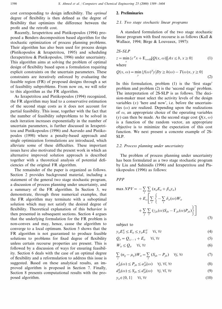
Fig. 2. Processing network of example 2.

for the feasibility and the subproblems are all zero,hence the master problem reduces to the form:min{m �m]0x, 05xB9}. The solution of this problemis clearly LB=0. Since UB=LB, the FR algorithmterminates with the solution x=0 and an objectivevalue of 0.

However, with a first stage solution of x=7.5, thefeasibility problems produce the feasible region of v asV. = [0, 7.5]. Using a five point quadrature over thisinterval, the quadrature points are calculated as vq=(0.35, 1.73, 3.75, 5.77, 7.15). Solving the subproblems ateach of these quadrature points and evaluating theexpectation, we find EV. [Q(7.5, v)]= −2.81. Thus, x=7.5 with the overall objective of −2.81 provides abetter solution than x=0. Thus, the FR algorithm hasproduced a solution which is not a global optimum tothe underlying problem.

3.2. Fixed degree of flexibility

In this subsection, we consider the case in which weare interested in obtaining a first stage decision of2S-SLP that is feasible for all realizations of the uncer-tain parameters. At its conception, the FR algorithmwas not intended for the case of fixed degree of flexibil-ity. We are here interested in examining the behavior ofthis algorithm if one insists in following the avenue ofthe FR algorithm in this context.

Consider the simple processing network of Fig. 2with two processes producing a single product. In stage1, we have to decide on the capacity levels of the twoprocesses. The cost per unit capacity of process 1 andprocess 2 are 2 and 1, respectively. Other productiongoals require a total capacity at least 20. In stage 2, theoperating level of the two processes should satisfy thestochastic demand v of the product. The operating costof Process 1 is 1, and that of process 2 is 0. Thus clearlyprocess 2 dominates process 1 and process 1 will onlybe operated to satisfy any unmet demand. The problemcan be formulated as follows.

Example 2

min 2x1+x2+EV[Q(x1, x2, v)]s.t. x1+x2]20x1, x2]0

where

Q(x1, x2, v)=min ys.t. y5x1

(17)

y]v−x2

y]0(18)

where

Q(x, v)=min −2y1+y2

s.t. y1+2y252x−v (14)

2y1+y25v−x+15 (15)

y1]v (16)

y1, y2]0

and

v�U(0, 30), i.e. V= [0, 30].

In the above formulation, x is the capacity/operatinglevel of process 0, y1 is the operating level of process 1and y2 is the operating level of process 2. Note that theoperating level of process 3 must be at least v. Con-straint (14) expresses the mass balance of product P0.The inequality is used to allow for inventory of theproducts. Similarly, constraint (15) expresses the massbalance of product P4. Constraint (16) enforces theminimum production requirement of product P3.

Let us now apply the FR algorithm to the aboveexample problem. We start with an initial solutionx=0. The feasibility problems to determine the feasiblerange of v are given by:

min/max v

s.t. y1+2y252x−v

2y1+y25v−x+15

y1]v

05v530

For the initial first stage solution of x=0, the abovefeasibility problem produces the feasible space for v asQ. ={0}. Since the feasibility space is a singleton, thesubproblem to be solved is:

Q(0, 0)=min−2y1+y2

s.t. y1+2y2502y1+y2515y1, y2]0

The solution to the above is y1=0 end y2=0. ThenUB=EV. [Q(x, w)]=0. The corrected dual multipliers


and

v�U(0, 30), i.e. V= [0, 30].

The variables x1 and x2 are the capacity levels ofprocess 1 and process 2, and y is the operating level ofprocess 1. Constraint (17) enforces the condition thatthe operating level of process 1 should not exceed itscapacity. Constraint (18) ensures that the minimumdemand of the final product is satisfied.

In the above problem, the required degree of flexibil-ity is the entire range V. Again, let us go through theFR algorithm step-by-step. We start with an initialsolution x1=0, x2=20. The feasibility problems todetermine the feasible range of the uncertain parame-ters are given by:

min/max v

s.t. y5x1

y]v−x2

y]0

05v530

For the initial solution x1=0, x2=20, the above prob-lems produce the feasible space of w as V. = [0, 20].Using a five-point quadrature in this interval, we findthe quadrature points vq= (0.938, 4.620, 10.000,15.380, 19.062). The subproblem to be solved at each ofthe quadrature points is:

min Q(0, 20, vq)={y �y50, y]vq−20, y]0}.

The solution at each of the quadrature points is, clear-ly, y=0. Then, UB=(2×0+20)+EV. [Q(0, 20, v)]=20. The corrected dual multipliers from the subprob-lems solved at each of the quadrature points areall zero. The master problem, then, reduces to theform:

min{m �m]2x1+x2, x1+x2]20, x1, x2]0}.

The solution of this problem is LB=m=20. SinceUB=LB, the algorithm terminates with the solution(x1=0, x2=20) as the optimal solution.

Note, however, that the range of possible values of v

for this problem is [0, 30] and that, for any v\20, thesolution (x1=0, x2=20) is infeasible. Thus, the FRalgorithm has produced the solution (x1=0, x2=20)which does not satisfy the pre-specified degree offlexibility.

3.3. Optimal degree of flexibility

In this subsection, we demonstrate that the FR al-gorithm may identify a solution that minimizes theexpected cost while disregarding flexibility.

Consider example 2 without the requirement of aminimum total capacity, i.e. the following problem:

Example 3

min 2x1+x2+EV[Q(x1, x2, v)]s.t. x1, x2]0

where

Q(x1, x2, v)=min ys.t. y5x1

y]v−x2

y]0

and

v�U(0, 30), i.e. V= [0, 30]

We start with an initial first stage feasible solution ofx1=0, x2=0. The feasibility problems to determine thefeasible range of the uncertain parameters are given by:

min/max v

s.t. y5x1

y]v−x2

y]0

05v530

For the initial solution x1=0, x2=0, the above prob-lems produce the feasible space of w as V. ={0}. Sincethe feasibility space is a singleton, the subproblem to besolved is:

Q(0, 20, 0)=min{y �y50, y]0−20, y]0}

The solution is, clearly, y=0. Then, UB= (2×0+0)+EV. [Q(0, 20, v)]=0. The corrected dual multipliervector from the feasibility and the subproblems are allzero. The master problem, therefore, reduces to theform:

min{m �m]2x1+x2, x1, x2]0}.

The solution of this problem is LB=m=0. SinceUB=LB, the algorithm terminates with the solution(x1=0, x2=0) as the optimal solution.

Note, that this solution is feasible only at a singlepoint in the random parameter space. The stochasticflexibility (Pistikopoulos & Mazzuchi 1990; Straub &Grossmann 1990) of a plan is the probability of theregion over which a plan is feasible. Clearly, the planidentified by the FR algorithm has a flexibility of 0(recall that we have a continuous distribution). On theother hand, the expected cost has been minimized tothe lowest value the first stage constraints permit. Thisexample, then, shows that the FR algorithm considersonly the expectation objective while entirely disregard-ing flexibility.

As the above three examples have demonstratedthree potential pitfalls of the FR algorithm, we nextaddress the question of whether the above algorithmcan be modified to overcome these weaknesses. Weconsider each of the three issues separately.


4. Convexity analysis

Example 1 demonstrated that different startingpoints might lead to different solutions when the FRalgorithm is used. This is counterintuitive as the firstand second stage problems are both linear for thisexample. In this section, we seek a theoretical explana-tion of this behavior. Recall that the optimizationproblem addressed by the FR algorithm is:

FR

z=minx

cTx+Ev�V. [Q(x, v)]

s.t. Ax5b, x]0

v�V.

where V. ={v�V�Q(x, v)B�}.For simplicity, consider a problem with a single

uncertain parameter. The second part of the objectivefunction of the above problem is given by:

Ev�V. [Q(x, v)]=& vU

v L

Q(x, v) d(P).

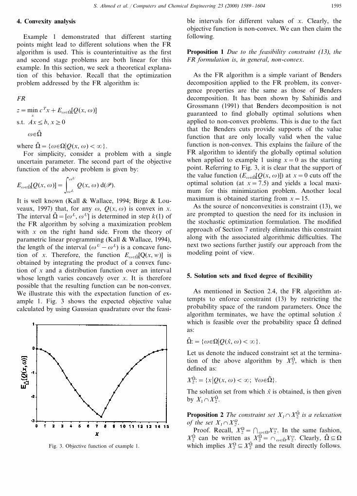
It is well known (Kall & Wallace, 1994; Birge & Lou-veaux, 1997) that, for any v, Q(x, v) is convex in x.The interval V. = [vL, vU] is determined in step k(1) ofthe FR algorithm by solving a maximization problemwith x on the right hand side. From the theory ofparametric linear programming (Kall & Wallace, 1994),the length of the interval (vU−vL) is a concave func-tion of x. Therefore, the function Ev�V. [Q(x, w)] isobtained by integrating the product of a convex func-tion of x and a distribution function over an intervalwhose length varies concavely over x. It is thereforepossible that the resulting function can be non-convex.We illustrate this with the expectation function of ex-ample 1. Fig. 3 shows the expected objective valuecalculated by using Gaussian quadrature over the feasi-

ble intervals for different values of x. Clearly, theobjective function is non-convex. We can then claim thefollowing.

Proposition 1 Due to the feasibility constraint (13), theFR formulation is, in general, non-con6ex.

As the FR algorithm is a simple variant of Bendersdecomposition applied to the FR problem, its conver-gence properties are the same as those of Bendersdecomposition. It has been shown by Sahinidis andGrossmann (1991) that Benders decomposition is notguaranteed to find globally optimal solutions whenapplied to non-convex problems. This is due to the factthat the Benders cuts provide supports of the valuefunction that are only locally valid when the valuefunction is non-convex. This explains the failure of theFR algorithm to identify the globally optimal solutionwhen applied to example 1 using x=0 as the startingpoint. Referring to Fig. 3, it is clear that the support ofthe value function (Ev�V. [Q(x, v)]) at x=0 cuts off theoptimal solution (at x=7.5) and yields a local maxi-mum for this minimization problem. Another localmaximum is obtained starting from x=15.

As the source of nonconvexities is constraint (13), weare prompted to question the need for its inclusion inthe stochastic optimization formulation. The modifiedapproach of Section 7 entirely eliminates this constraintalong with the associated algorithmic difficulties. Thenext two sections further justify our approach from themodeling point of view.

5. Solution sets and fixed degree of flexibility

As mentioned in Section 2.4, the FR algorithm at-tempts to enforce constraint (13) by restricting theprobability space of the random parameters. Once thealgorithm terminates, we have the optimal solution x̂which is feasible over the probability space V. definedas:

V. :={v�V�Q(x̂, v)B�}.

Let us denote the induced constraint set at the termina-tion of the above algorithm by X2

V. , which is thendefined as:

X2V. :={x �Q(x, v)B�; Öv�V. }.

The solution set from which x̂ is obtained, is then givenby X1SX2

V. .

Proposition 2 The constraint set X1SX2V. is a relaxation

of the set X1SX2V.

Proof. Recall, X2V=�v�VX2

v. In the same fashion,X2

V. can be written as X2V. =Sv�V. X2

v. Clearly, V. ¤Vwhich implies XV

2¤X2V. and the result directly follows.Fig. 3. Objective function of example 1.


It is thus clear that the solution, x̂, produced by theFR algorithm is a point from the relaxed solution spacerather than the desired space X1SXV

2 . This solutionmay not be feasible to the original problem for therequired degree of flexibility. This is very clear intu-itively, since the solution x̂ is feasible only for a subsetof the entire probability space of the random parame-ters and might not be feasible for some other realiza-tion of the parameters

Proposition 3 If the problem has complete recourse orrelati6ely complete recourse property, then X1SX2

V. =X1SXV

2 .Proof. If either of the properties holds, then

X1SXV2 =X1. If the problem has complete recourse,

then XV2 =R

n1. Also, from proposition 2, XV2¤X2

V. . Itthus follows that XV

2 =Rn1 and X1SXV

2 =X1=X1SXV

2 . If the problem has relatively complete re-course, then X1¤XV

2 . Since XV2¤X2

V ., we haveX1SX2

V. =X1=X1SXV2 .

Example 2 in Section 3 did not possess the relativelycomplete recourse property and the FR algorithm pro-duced a solution that is not feasible over the entirerange of uncertain parameters. Thus, from proposition3, we can say that the feasibility of a solution x̂�X2

V. isguaranteed if the problem has the complete or relativelycomplete recourse property. In general, however, thisproperty is not present in the given problem and mustbe enforced. Two possible ways for achieving this arepresented in the next subsection.

5.1. Enforcing relati6ely complete recourse

Per Section 2.3, the solution space of a problemhaving relatively complete recourse is the explicit firststage constraint set X1. Two different classes ofalgorithms have been developed for 2S-SLP, de-pending upon the presence or absence of the recourseproperty.

Decomposition approaches such as the L-shapedmethod of Van Slyke and Wets (1969) and the regu-larized decomposition method of Ruszczynski (1986)are applicable to problems without relatively completerecourse. These methods start with a candidate solutionfrom X1, and test this solution against all possiblerealizations of the random parameters. If any infeasibil-ities arise, feasibility cuts are added to X1 to chop offthe ‘bad’ solution point. Thus, X1 is iteratively modifiedby the addition of feasibility cuts until it satisfies therelatively complete recourse property.

Another class of algorithms includes the ones thatassume relatively complete recourse in the problem.Sampling-based algorithms for stochastic programminglike the stochastic decomposition method of Higle andSen (1991) and the stochastic quasi-gradient method of

Ermoliev (1983), fall under this category. These meth-ods solve the problem for a sampled set of realizationsof the uncertain parameters. Hence, it is extremelyimportant to ensure that the solution obtained will notbe infeasible for some other realizations of theseparameters. If relatively complete recourse is notpresent in the problem, it must be enforced before thesemethods can be applied.

It follows from propositions 2 and 3 that, enforcingrelatively complete recourse by restricting the probabil-ity space of the random parameters results in a relax-ation of the problem, and that the solution producedmay not be feasible unless the problem already pos-sesses the recourse property. To make the FR al-gorithm provide a feasible solution, relatively completerecourse must be enforced through modification of thefirst stage constraint set. It is now shown how this canbe achieved in both an iterative fashion as well as apriori.

5.1.1. Feasibility cutsRelatively complete recourse can be enforced in an

iterative manner by the addition of feasibility cuts(when needed) in each iteration. The FR algorithmneeds to be modified as follows. The entire probabilityspace of the random parameters needs to be considered.Thus, we do not have to solve the feasibility problemsin step k(1) of the algorithm. In step k(2), the quadra-ture points are to be determined for the entire range V.While solving the subproblems in step k(3), if anyinfeasibilities arise, a feasibility cut has to be con-structed and added to X1 to chop off the current iterate.The new master problem has to be solved and theprocedure should start from step k(1) with the newsolution. If the subproblem corresponding to vq andthe current iterate xk is infeasible, and p are the extremedual directions for this problem, then the feasibility cutis given by (e.g. Infanger (1994)):

p [h(vq)−T(vq)x ]50.

A formal statement of the modified algorithm is pre-sented in Section 7. It should be noted that, whilechecking for infeasibilities and generating cuts, the en-tire probability space V has to be exhausted. Therefore,the choice of the quadrature points is very important.In particular, since if a solution is infeasible for anypoint in the probability space, it must be infeasible foran extreme point of the probability space (Swaney &Grossmann, 1985; Kall & Wallace, 1994), the quadra-ture points should include the extreme points of thespace of the random vector. If each component of therandom vector is independent of each other, then theextreme points of the probability space are given by allpossible combinations of the upper and lower boundsof each component of the random vector.


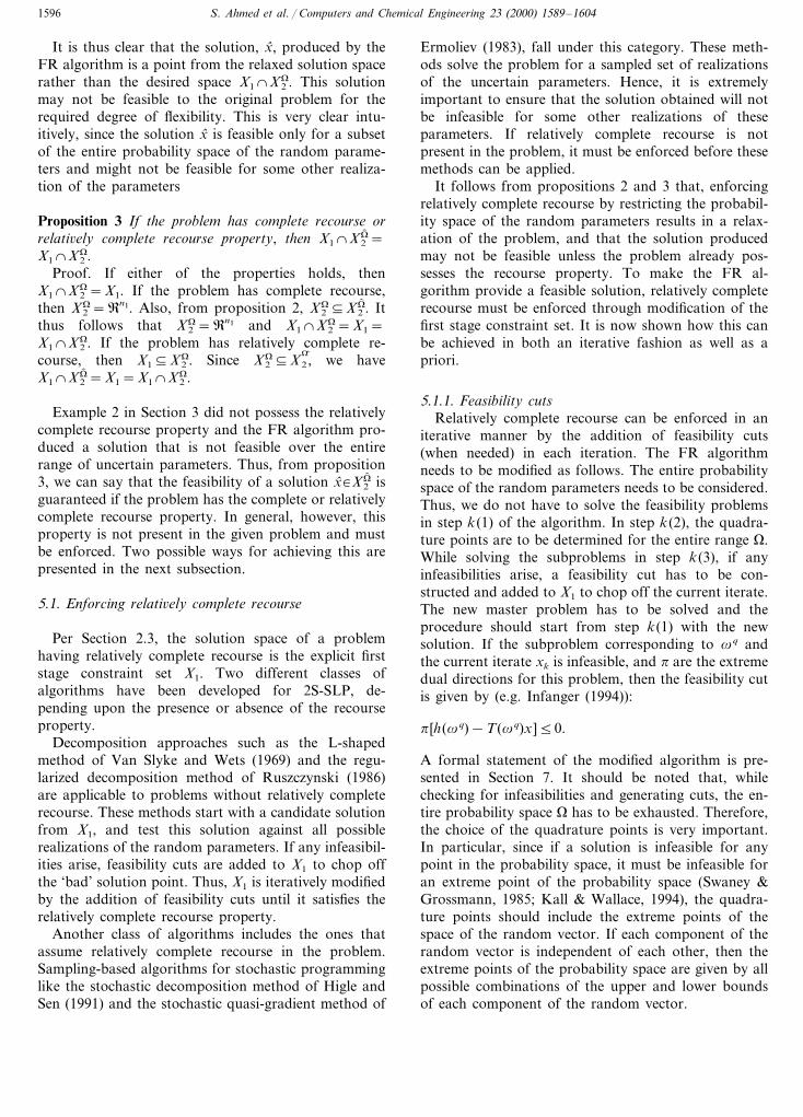
Fig. 4. Effect of reducing probability space.

flexible one. In this section, we address the problem ofseeking an optimal degree of flexibility, i.e. balancingthe trade-offs between economic optimality and in-creased plan flexibility. Example 3 in Section 3 demon-strated that the FR algorithm may identify a solutionthat minimizes the expected cost while minimizing,instead of attempting to maximize flexibility. This ex-ample shows that the FR algorithm considers only theexpectation objective, while entirely disregarding flexi-bility. This is due to an underestimation of the actualcost as proved next.

Recall that the standard two stage stochastic pro-gramming problem is:

(P1): zV= minx�X 1SX 2

V{cTx+Ev�V[Q(x, v)]}

and the problem considered by the FR algorithm afterrestricting the probability space to V. is:

(P2): zV. = minx�X 1SX 2

V.{cTx+Ev�V. [Q(x, v)]}.

If the second stage problem is bounded, we can alwaysredefine the recourse cost function and make it positiveby translating it by a constant amount without chang-ing the optimal solution of the problem. Therefore,without loss of generality, we may assume that therecourse costs are nonnegative.

Proposition 4 If Q(x, v)]0, then zV. 5zV for any V. ¤V.Proof. From proposition 2, if V. ¤V, then X1SX2

V. ±X1SXV

2 . Also, for any solution feasible to P1, theobjective function value is given by:

cTx+&

VQ(x, v) d(P)

=cTx+&

V.Q(x, v) d(P)+

&V−V.

Q(x, v) d(P)

]cTx+&

V.Q(x, v) d(P)

It is thus clear that problem (P2) is a relaxation of(P1), and therefore zV. 5zV.

The above proposition clearly shows that restrictingthe probability space corresponds to reducing the objec-tive value. In fact, decrease in the expected cost ispossible by reducing the probability space until X2

V. ±X1. This fact is illustrated by example 3 and Fig. 4.Since the FR algorithm works by restricting the proba-bility space in each iteration, it reduces the flexibilityand improves the expectation objective without consid-ering the trade-offs.

6.1. Combining the conflicting objecti6es

The contribution of the flexibility cost is not consid-ered in the objective of the problem considered by the

5.1.2. A priori recourseRelatively complete recourse can be enforced a priori

through the addition of the ‘worst case’ constraints ofthe second stage to the first stage fixed constraint setX1. There is no standard rule to identify such con-straints as these depend on the structure of the prob-lem. In Liu and Sahinidis (1996), the authors suggesthow this can be done in the problem PPP. Note that, inPPP, the uncertainties are only in the bounds of thesecond stage variables. Additionally, the uncertainparameters are linear functions of the random vector v,and each component of the random vector is indepen-dent. Under these conditions, addition of the followingconstraints to X1 guarantees relatively complete re-course in the problem:

W( it5Qit Öi

%i

(hij−mij)W( it=%l

(S( jlt−P( jlt) Öj, Öt

maxV

ajltL (v)5P( jlt5min

Vajlt

U(v) Öj, Öl, Öt

maxV

djltL (v)5S( jlt5min

Vdjlt

U(v) Öj, Öl, Öt

Note that some new variables (W( it, P( jlt, S( jlt) have beenintroduced to the master problem.

The modified FR algorithm, as stated in Section 7,can be used to solve PPP after enforcing relativelycomplete recourse in the above manner. However, thereis no need for the feasibility cuts, as, in this case, everyfirst stage solution x leads to a feasible second stageproblem.

6. Trading cost for flexibility

In most practical problems, the expected cost andflexibility objectives are conflicting — a more flexibleplan is more likely to be more expensive than a less


FR algorithm. Consequently, the algorithm strives tominimize the expected cost while measuring the regionof feasibility, rather than optimizing it. In order tocombine the two conflicting objectives of minimizingexpected cost and maximizing flexibility, we have tomodify the objective function of 2S-SLP in order toreflect the trade-offs associated with the cost andflexibility.

Such an approach is taken in the paper by Pistiko-poulos and Grossmann (1988). Here, the authors cap-ture the trade-offs between expected profit andflexibility, by associating a retrofit cost with a flexibledesign. The optimal degree of flexibility is then definedas one that maximizes the difference between the ex-pected profit and the expected retrofit cost. A similarapproach was taken by Ierapetritou and Pistikopoulos(1996) and Epperly, Ierapetritou and Pistikopoulos(1997). In the same spirit, in the context of (2S-SLP),we can include recourse variables with a penalty cost tothe second stage problem to guarantee feasibility. Themodified second stage problem is then given by:

Q %(x, v)=miny { f(v)Ty+p(v)Ts �Dy+s]h(v)

−T(v)x, y]0} (19)

The penalty cost is a measure of the in-flexibility of aplan x and including this in the objective functionaccounts for the trade-offs between minimizing costand maximizing flexibility. This, after all, is the mainphilosophy of two stage stochastic programming withrecourse. For the process-planning problem, the cost ofoutsourcing production may be thought of as the re-course cost. In particular, the recourse variables can bethought of as the amount of a chemical that is pur-chased from outside vendors at the corresponding out-sourcing cost in order to satisfy demand that exceedsthe in-house capacity. Clearly, the modified secondstage problem is guaranteed to be feasible for any valueof x and v.

Proposition 5 Problem (2S-SLP) with the modified re-course function Q % has the complete recourse property.

Since we have enforced a priori recourse, themodified problem can now be solved using the im-proved FR algorithm stated in Section 7. The region offlexibility of the optimal solution of the modified prob-lem (x*, y*) can then be determined through feasibilitysubproblems corresponding to the original second stageproblem Q, as suggested by Straub and Grossmann(1993).

7. The improved algorithm

The previous sections have shown that the inclusion

of constraint (13) in the FR formulation renders itnon-convex. Moreover, this constraint on the uncertainparameters results in solutions that may fail to satisfyfixed or optimal degree of flexibility. We thereforepropose to modify the FR algorithm to address theformulation 2S-SLP instead of the FR formulation. Forsimplicity of the exposition, first consider the followingtwo stage stochastic program with a single uncertainparameter.

z=minx

cTx+Ev�V[Q(x, v)]s.t. Ax5b, x]0

where

Q(x, v)=miny

{ f(v)Ty �Dy]h(v)−T(v)x, y]0}.

Since we are evaluating the expectation by Gaussianquadrature, the uncertain parameter space needsto be bounded to be able to place the quadraturegrid points. It should be mentioned that Monte Carlointegration schemes circumvents this problem bysampling from the entire domain of the distributionfunction. The bounds on the uncertain par-ameters, V= [vL, vU], can be obtained from the de-sired confidence intervals, for example, m94s for nor-mal distributions. The first stage constraint set Ax5b,x]0 may also include a priori recourse constraintswhen applicable. The quadrature points in V need to beevaluated only once. These are obtained by the formu-las:

wq=0.5[vU(1+6q)+vU(1−6q)] q=1, ... , Q(

where Q( is the number of quadrature points and 6q arethe roots. With this discretization of the uncertainparameter space, we can now state the modifiedalgorithm.

The impro6ed algorithm

Step 0Select an initial plan x0, k�0, UB= +�, LB= −�.Step k(1)Solve the stage-2 subproblems Q(xk, vq) at each ofthe Q( quadrature points. If the subproblem corre-sponding to vk is infeasible, use the extreme dualdirection pk to add the following feasibility to cut tothe master problem:

pk [h(vk)−T(vk)x ]50

and go to step k(4) otherwise go to step k(2).Step k(2)Evaluate the upper bound using Gaussianquadrature:


UBk=cTxk+vU−vL

2%Q(

q=1

uq×Q(xk, vq)×J(vq)

where uq are the weights associated with quadraturepoints and J(vq) is the probability distribution func-tion. If UBkBUB, then let UB=UBk and x*=xk.Step k(3)Let pk,q are the optimal dual solutions from thesubproblems in step k(1). Add the following optimal-ity cut to the master problem:

m]cTxk+vU−vL

2%Q(

q=1

uq×pk,q [h(vq)−T(vq)x ]

×J(vq).

Step k(4)Solve the following master problem to get the lowerbound:

LB=min m (20)

s.t. Ax5b, x]0 (21)

m]cTxk+vU−vL

2%Q(

q=1

uq×pl,q [h(vq)−T(vq)x ]

×J(vq) l=1, k (22)

pl [h(v l)−T(v l)x ]50 l=1, k (23)

Constraints (22) and (23) are the optimality and thefeasibility cuts, respectively.Step k(5)If UB−LB5e STOP, x* is the optimal solution;else set k�k+1, xk+1=xk and repeat from stepk(1).

The initial plan x0 need only satisfy the first stageconstraint set. This can be obtained by solving the mean6alue problem, where the uncertain parameters are re-placed by their mean values resulting in a deterministicprogram.

In the above algorithm, the feasibility cuts are itera-tively enforced as described in Section 5.1. For the casewhen a priori recourse has been enforced, the algorithmdoes not require the feasibility cuts. For the purpose ofexposition, only a single uncertain parameter was con-sidered above. This is in no way restrictive, since addi-tional uncertain parameters can be accommodatedthrough multidimensional Gaussian quadrature whileevaluating the expectation.

8. Computational experiments

The algorithm of Section 7 has been coded in GAMS(Brook, Kendrick & Meeraus, 1988) using MINOS to

solve linear programs and ZOOM for mixed integerprograms. All computations were carried out on a SunSPARC 2 workstation. The modeling language, thehardware and example problems used are identical tothat used by Ierapetritou and Pistikopoulos (1994). Inparticular, examples 4 and 5 correspond to examples 1and 2, respectively of Ierapetritou and Pistikopoulos(1994).

Example 4

This example involves only two random parameters,vl and v2:

max profit=100S13+80S14+10I11f +15I12

f +20I13f

+25I14f −10P11−15P12−10P21−15P22

−30R11−35R12+90S23+80S24+10I21f

+15I22f +25I23

f +20I24f −30R21−35R22

−10I22in −I22

in −30I23in −30I24

in (24)

subject to

Pk1+Ik1in =0.4Rk1+Ik1

f k=1,2 (25)

Pk2+Ik2in =0.6Rk1+Rk2+Ik2

f k=1, 2 (26)

Ik3in +0.5Rk1=Ik3

f +Sk3 k=1, 2 (27)

Ik4in +0.6Rk2=Ik4

f +Sk4 k=1, 2 (28)

205Rk15100 k=1, 2 (29)

305Rk25100 k=1, 2 (30)

205P115100 (31)

305P125200 (32)

205P215200 (33)

105P225v1 (34)

205S13540 (35)

205S14585 (36)

v25S23540 (37)

205S24585 (38)

05Ikjf k=1, 2; j=1, 4 (39)

I1jin=0 j=1, 4 (40)

I1jf =I2j

in j=1, 4 (41)

The problem formulation involves two decision stages(k=1, 2), four chemicals ( j=1, 4), and two processes(i=1, 2). The problem is stated in terms of purchases(Pkj), sales (Skj), operating levels (Rkj), and initial andfinal inventories (I in

kj, I fkj). The corresponding chemical

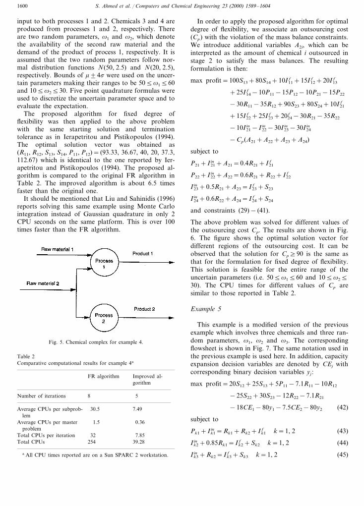
complex is shown in Fig. 5. As shown in this figure,chemical 1 is input to process 1, whereas chemical 2 is


input to both processes 1 and 2. Chemicals 3 and 4 areproduced from processes 1 and 2, respectively. Thereare two random parameters, v1 and v2, which denotethe availability of the second raw material and thedemand of the product of process 1, respectively. It isassumed that the two random parameters follow nor-mal distribution functions N(50, 2.5) and N(20, 2.5),respectively. Bounds of m94s were used on the uncer-tain parameters making their ranges to be 505v1560and 105v2530. Five point quadrature formulas wereused to discretize the uncertain parameter space and toevaluate the expectation.

The proposed algorithm for fixed degree offlexibility was then applied to the above problemwith the same starting solution and terminationtolerance as in Ierapetritou and Pistikopoulos (1994).The optimal solution vector was obtained as(R11, R12, S13, S14, P11, P12)= (93.33, 36.67, 40, 20, 37.3,112.67) which is identical to the one reported by Ier-apetritou and Pistikopoulos (1994). The proposed al-gorithm is compared to the original FR algorithm inTable 2. The improved algorithm is about 6.5 timesfaster than the original one.

It should be mentioned that Liu and Sahinidis (1996)reports solving this same example using Monte Carlointegration instead of Gaussian quadrature in only 2CPU seconds on the same platform. This is over 100times faster than the FR algorithm.

In order to apply the proposed algorithm for optimaldegree of flexibility, we associate an outsourcing cost(Cp) with the violation of the mass balance constraints.We introduce additional variables A2i, which can beinterpreted as the amount of chemical i outsourced instage 2 to satisfy the mass balances. The resultingformulation is then:

max profit=100S13+80S14+10I11f +15I12

f +20I13f

+25I14f −10P11−15P12−10P21−15P22

−30R11−35R12+90S23+80S24+10I21f

+15I22f +25I23

f +2024f −30R21−35R22

−10I21in −I22

in −30I23in −30I24

in

−Cp(A21+A22+A23+A24)

subject to

P21+I21in +A21=0.4R21+I21

f

P22+I22in +A22=0.6R21+R22+I22

f

I23in +0.5R21+A23=I23

f +S23

I24in +0.6R22+A24=I24

f +S24

and constraints (29)− (41).

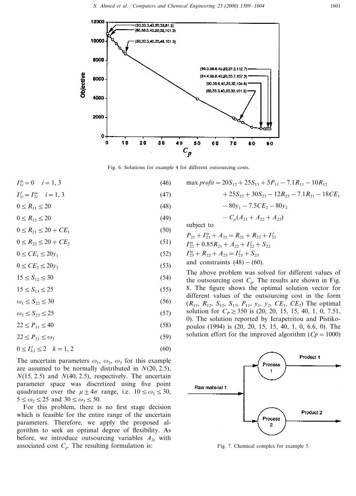
The above problem was solved for different values ofthe outsourcing cost Cp. The results are shown in Fig.6. The figure shows the optimal solution vector fordifferent regions of the outsourcing cost. It can beobserved that the solution for Cp]90 is the same asthat for the formulation for fixed degree of flexibility.This solution is feasible for the entire range of theuncertain parameters (i.e. 505v1560 and 105v2530). The CPU times for different values of Cp aresimilar to those reported in Table 2.

Example 5

This example is a modified version of the previousexample which involves three chemicals and three ran-dom parameters, v1, v2 and v3. The correspondingflowsheet is shown in Fig. 7. The same notation used inthe previous example is used here. In addition, capacityexpansion decision variables are denoted by CEj withcorresponding binary decision variables yj :

max profit=20S12+25S13+5P11−7.1R11−10R12

−25S22+30S23−12R22−7.1R21

−18CE1−80y1−7.5CE2−80y2 (42)

subject to

Pk1+Ik1in =Rk1+Rk2+Ik1

f k=1, 2 (43)

Ik2in +0.85Rk1=Ik2

f +Sk2 k=1, 2 (44)

Ik3in +Rk2=Ik3

f +Sk3 k=1, 2 (45)

Fig. 5. Chemical complex for example 4.

Table 2Comparative computational results for example 4a

FR algorithm Improved al-gorithm

8 5Number of iterations

30.5 7.49Average CPUs per subprob-lem

0.361.5Average CPUs per masterproblem

Total CPUs per iteration 32 7.85Total CPUs 254 39.28

a All CPU times reported are on a Sun SPARC 2 workstation.


Fig. 6. Solutions for example 4 for different outsourcing costs.

I1iin=0 i=1, 3 (46)

I1if =I2i

in i=1, 3 (47)

05R11520 (48)

05R12520 (49)

05R21520+CE1 (50)

05R22520+CE2 (51)

05CE1520y1 (52)

05CE2520y2 (53)

155S12530 (54)

155S13525 (55)

v15S22530 (56)

v25S23525 (57)

225P11540 (58)

225P215v3 (59)

05Ik1f 52 k=1, 2 (60)

The uncertain parameters v1, v2, v3 for this exampleare assumed to be normally distributed in N(20, 2.5),N(15, 2.5) and N(40, 2.5), respectively. The uncertainparameter space was discretized using five pointquadrature over the m94s range, i.e. 105v1530,55v2525 and 305v3550.

For this problem, there is no first stage decisionwhich is feasible for the entire range of the uncertainparameters. Therefore, we apply the proposed al-gorithm to seek an optimal degree of flexibility. Asbefore, we introduce outsourcing variables A2i withassociated cost Cp. The resulting formulation is:

max profit=20S12+25S13+5P11−7.1R11−10R12

+25S22+30S23−12R22−7.1R21−18CE1

−80y1−7.5CE2−80y2

−Cp(A21+A22+A23)subject to

P21+I21in +A21=R21+R22+I21

f

I22in +0.85R21+A22+I22

f +S22

I23in +R22+A23=I23

f +S23

and constraints (48)− (60).

The above problem was solved for different values ofthe outsourcing cost Cp. The results are shown in Fig.8. The figure shows the optimal solution vector fordifferent values of the outsourcing cost in the form(R11, R12, S12, S13, P11, y1, y2, CE1, CE2) The optimalsolution for CP]350 is (20, 20, 15, 15, 40, 1, 0, 7.51,0). The solution reported by Ierapetritou and Pistiko-poulos (1994) is (20, 20, 15, 15, 40, 1, 0, 6.6, 0). Thesolution effort for the improved algorithm (Cp=1000)

Fig. 7. Chemical complex for example 5.


Fig. 8. Solutions for example 5 for different values of outsourcing cost.

Table 3Comparative computational results for example 5a

Improved al-FR algorithmgorithm

Number of iterations 75

199Average CPUs per subprob- 45.21lem

Average CPUs per master 3 0.47problem

Total CPUs per iteration 205 45.67319.71025Total CPUs

a All CPU times reported are on a Sun SPARC 2 workstation.

multiple minima difficulty while it accurately accountsfor the trade-offs between cost and flexibility.

Acknowledgements

This work was in part supported by the NationalScience Foundation under CAREER award DMII 95-02722 to N.V.S.

Appendix A. Notation

IndicesI For the set of processes that consti-

tutes the network.For the set of chemicals that inter-jconnect the processes.

l For the set of markets for purchaseand sale of chemicals.For the set of quadrature points.qFor the set of time periods of thetplanning horizon.

Variablesp Dual vector from the subproblem.m Variable representing total cost in

master problem.Units of expansion of process i at theEit

beginning of period t.Units of chemical j purchased fromPjlt

market l at the beginning of period tunder scenario k.

Qit Total capacity of process i in periodt.Units of chemical j sold to market lSjlt

at the end of period t.

and those reported by Ierapetritou and Pistikopoulos(1994) are compared in Table 3. The improved al-gorithm is about three times faster than the originalone. The MILP master problem were solved usingZOOM instead of SCICONIC as in Ierapetritou andPistikopoulos (1994).

9. Conclusions

The developments of this paper center around com-plete and relatively complete recourse properties of twostage stochastic programs in the context of processplanning under uncertainty. In particular, it is shownthat, if these properties are not satisfied, a decomposi-tion approach based on integration only over the feasi-ble space may get trapped at a suboptimal solution orlead to solutions that do not satisfy the desired degreeof flexibility. Remedial measures based on enforcingrecourse properties are suggested and lead to the devel-opment of an algorithm which does not suffer from the


Operating level of process i in periodWit

t.Vector of first stage variablesx

(x�Rn1).Vector of second stage variablesy

(y�Rn2)A 0–1 integer variable. If process i isyit

expanded during period t thenyit=1, else yit=0.

ParametersPer unit expansion cost for process iait

at the beginning of period t.Fixed cost of establishing or expand-bit

ing process i at the beginning ofperiod t.

Selling and buying prices of chemicalgjlt(v),Gjlt(v) j in market l in period t as a func-

tion of v.Unit production cost to operate pro-dit(v)

cess i during period t as a functionof v.

Input proportionality constant forhij

chemical j in process i.mij Output proportionality constant for

chemical j in process i.Random vector belonging to thev

probability space (V, S, P).Lower and upper bounds for theaL

jlt(v),aU

jlt(v) availability (purchase amount) ofchemical j in market l in period tas a function of v.

First stage constraint matrixA(A�Rm1×n1).

b First stage right hand side vector(b�Rm1).

c First stage cost vector (c�Rn1).dL

jlt(v), Lower and upper bounds for the de-mand (sale amount) of chemical jdU

jlt(v)in market l in period t as a func-tion of v.

D Second stage recourse matrix(D�Rm2×n2).

ELit, EU

it Lower and upper bounds for the ca-pacity expansion of process i in pe-riod t.

Second stage right hand side vectorh(v)as a function of v (h(v)�Rm2).

Second stage technology matrix as aT(v)function of v(T(v)�Rm2×n1).

uq Weights in the quadrature formula.Roots in the quadrature formula.6q

Sets and functions

Set of all possible values of the ran-Vdom variable v.

S The collection of all subsets of Q.The probability density function ofJ(v)

the random variable v.The probability measure of the ran-P

dom variable v.Q(·) The second stage cost function.

The first stage ‘fixed’ constraint set.X1

The second stage constraint set forXv2

given v.The second stage ‘induced’ constraintXV

2

set.

References

Acevedo, J., & Pistikopoulos, E. N. (1998). Stochastic optimizationbased algorithms for process synthesis under uncertainty. Com-puters & Chemical Engineering, 22, 647–671.

Birge, J. R., & Louveaux, F. (1997). Introduction to stochastic pro-gramming. New York, NY: Springer.

Brook, A., Kendrick, D., & Meeraus, A. (1988). GAMS — a user ’sguide. Redwood City, CA: Scientific Press.

Clay, R. L., & Grossmann, I. E. (1997). A disaggregation algorithmfor the optimization of stochastic planning models. Computers &Chemical Engineering, 21, 751–774.

Epperly, T., Ierapetritou, M., & Pistikopoulos, E. (1997). On theglobal and efficient solutions of stochastic batch plant designproblems. Computers & Chemical Engineering, 21, 1411–1431.

Ermoliev, Y. (1983). Stochastic quasigradient methods and theirapplication to systems optimization. Stochastics, 9, 1–36.

Higle, J. L., & Sen, S. (1991). Stochastic decomposition: an algorithmfor two stage stochastic linear programs with recourse. Mathe-matics of Operations Research, 16, 650–669.

Ierapetritou, M. G., & Pistikopoulos, E. N. (1994). Novel optimiza-tion approach of stochastic planning models. Industrial Engineer-ing Chemistry Research, 33, 1930–1942.

Ierapetritou, M. G., & Pistikopoulos, E. N. (1996). Global optimiza-tion for stochastic planning, scheduling and design problems. In.I. Grossmann, Global Optimization in Engineering Design,Kluwer Academic Publishers, Boston, MA.

Infanger, G. (1994). Planning under uncertainty: sol6ing large scalestochastic linear programs. Danvers, MA: Boyd and Fraser.

Kall, P., & Wallace, S. W. (1994). Stochastic programming.Chichester, England: John Wiley and Sons.

Liu, M. L., & Sahinidis, N. V. (1996). Optimization in processplanning under uncertainty. Industrial & Engineering ChemistryResearch, 35, 4154–4165.

Pistikopoulos, E. N., & Grossmann, I. E. (1988). Stochastic optimiza-tion of flexibility in retrofit design on linear systems. Computers &Chemical Engineering, 12, 1215–1227.

Pistikopoulos, E. N., & Grossmann, I. E. (1989). Optimal retrofitdesign for improving process flexibility in non-linear systems —II. Optimal level of flexibility. Computers & Chemical Engineering,13, 1087–1096.

Pistikopoulos, E. N., & Ierapetritou, M. G. (1995). Novel approachfor optimal design under uncertainty. Computers & ChemicalEngineering, 19, 1089–1110.

Pistikopoulos, E. N., & Mazzuchi, T. A. (1990). A novel flexibilityanalysis approach for processes with stochastic parameters. Com-puters & Chemical Engineering, 14, 991–1000.

Ruszczynski, A. (1986). A regularized decomposition method forminimizing a sum of polyhedral functions. Mathematical Pro-gramming, 35, 309–333.


Sahinidis, N. V., & Grossmann, I. E. (1991). Convergence propertiesof generalized benders decomposition. Computers & ChemicalEngineering, 15, 481–491.

Straub, D. A., & Grossmann, I. E. (1990). Integrated stochastic metricof flexibility for systems with discrete state and continuous parame-ter uncertainties. Computers & Chemical Engineering, 14, 967–980.

Straub, D. A., & Grossmann, I. E. (1993). Design optimization ofstochastic flexibility. Computers & Chemical Engineering, 17, 339–354.

Swaney, R. E., & Grossmann, I. E. (1985). An index for operationalflexibility in chemical process design. Part 1: formulation andtheory. American Institute of Chemical Engineers Journal, 31,621–630.

Van Slyke, R., & Wets, R. (1969). L-shaped linear programs withapplications to optimal control and stochastic programming. SIAMJournal on Applied Mathematics, 17, 638–663.

Wets, R. (1966). Programming under uncertainty: the solution set.SIAM Journal on Applied Mathematics, 14, 1143–1151.

.

an improved decomposition algorithm for optimization under uncertainty

Documents