Computers FluidsVol. 23,No. 1, pp. 1–21, 1994

An Implicit Upwind Algorithm for ComputingTurbulent Flows on Unstructured Grids.

W. Kyle Anderson and Daryl L. Bonhaus

NASA Langley Research Center

Hampton, Virginia 23665–5225

An implicit, Navier-Stokes solution algorithm is presented for the computation of turbulent flow onunstructuredgrids. The inviscid fluxes are computed using an upwind algorithm and the solution is advancedin time using a backward-Eulertime-steppingscheme. At each time step, the linear system of equations isapproximately solved with a point-implicit relaxation scheme. This methodology provides a viable and robustalgorithm for computing turbulent flows on unstructured meshes.

Resultsare shown for subsonic flow over a NACA 0012 airfoil and for transonic flow over a RAE 2822airfoil exhibiting a strong upper-surfaceshock. In addition, results are shown for 3–element and 4–elementairfoil configurations. For the calculations,two one–equationturbulencemodels are utilized. For the NACA0012airfoil, a pressuredistributionandforce dataarecomparedwith othercomputationalresultsaswell aswithexperiment. Comparisons of computed pressure distributions and velocity profiles with experimental data areshown for the RAE airfoil and for the 3–element configuration. For the 4–element case, comparisons of surfacepressure distributions with experiment are made. In general, the agreement between the computations and theexperimentis good.

1. Introduction

For computing flows on complicated geometries such as multielement airfoils, the use of unstructured gridsoffers a good alternative to more traditional methods of analysis. This is primarily due to the promise of dramaticallydecreased time required to generate grids over complicated geometries. Also, unstructured grids offer the capabilityto locally adapt the grid to improve the accuracy of the computation without incurring the penalties associated withglobal refinement. While work remains to be done to fully realize their potential, much progress has been madein computing viscous flows on unstructured grids.

While several advanceshave been made for computing turbulent flow on unstructured grids (e.g. [1][2]), probably the most mature and widely used code for computing two-dimensional turbulent viscous flow onunstructured grids is that of Mavriplis [3]. In this reference, the solution algorithm is a Galerkin finite-elementdiscretization and a Runge-Kutta time-stepping algorithm is used in conjunction with multigrid to obtain veryefficient solutions. The turbulence model predominantly utilized in this code is that of Baldwin and Lomax [4]although extensions have been made to include a two-equation turbulence model [5]. Other modifications to thiscode are presented in reference [6] in which backward-Euler time-differencing is used in conjunction with GMRES[7] to produce results which are competitive with multigrid for the cases considered.

The use of upwind differencing offers several advantages over a central-differencing formulation for computingviscous flows. For example, in references [8] and [9], it is clearly shown that with the flux-differencing schemeof Roe [10] the resolution of boundary layer details typically requires only half as many points as with a central-differencing code. As discussed in reference [11], the poor performance of the central-difference formulation isattributed to the scalar artificial dissipation formulas commonly used to damp odd-even oscillations and to providenon-linear stability.

For upwind calculations on unstructured grids, Barth [12] has described methodology for utilizing Roe’sapproximate Riemann solver [10] for the inviscid flux computations and a Galerkin formulation for the viscousterms. In this work, a sparse matrix solver is used in conjunction with a Runge-Kutta time-stepping algorithm for

1

updating the solution at each time step. The turbulence model included is that of Baldwin-Barth [13] and samplecomputationsareshownover a single-elementairfoil as well as a two-element airfoil in a wind tunnel.

For the currentstudy,the flux-difference-splittingof Roe is used for computing the inviscid contribution to theflux and an implicit solver based on backward-Euler time differencing is utilized for updating the solution. At eachtime step, the linear system of equations is approximately solved with a red-black type relaxation procedure. Thismethod circumvents the need to assemble large matrices and, therefore, significantly reduces the required memory.As in reference [12], the Baldwin-Barth turbulence model is used for computing flows at high Reynolds number. Inaddition, a recently developed turbulence model due to Spalart and Allmaras [14] is also utilized and comparisonsbetween solutions obtained with each model are shown. Results are shown for subsonic flow over a NACA 0012airfoil and for transonic flow over a RAE 2822 airfoil as well as for the flow over two multielement airfoils. Detailedcomparisons are made with available experimental data. These comparisons include velocity profiles at particularlocations along the surface as well as pressure and skin friction distributions.

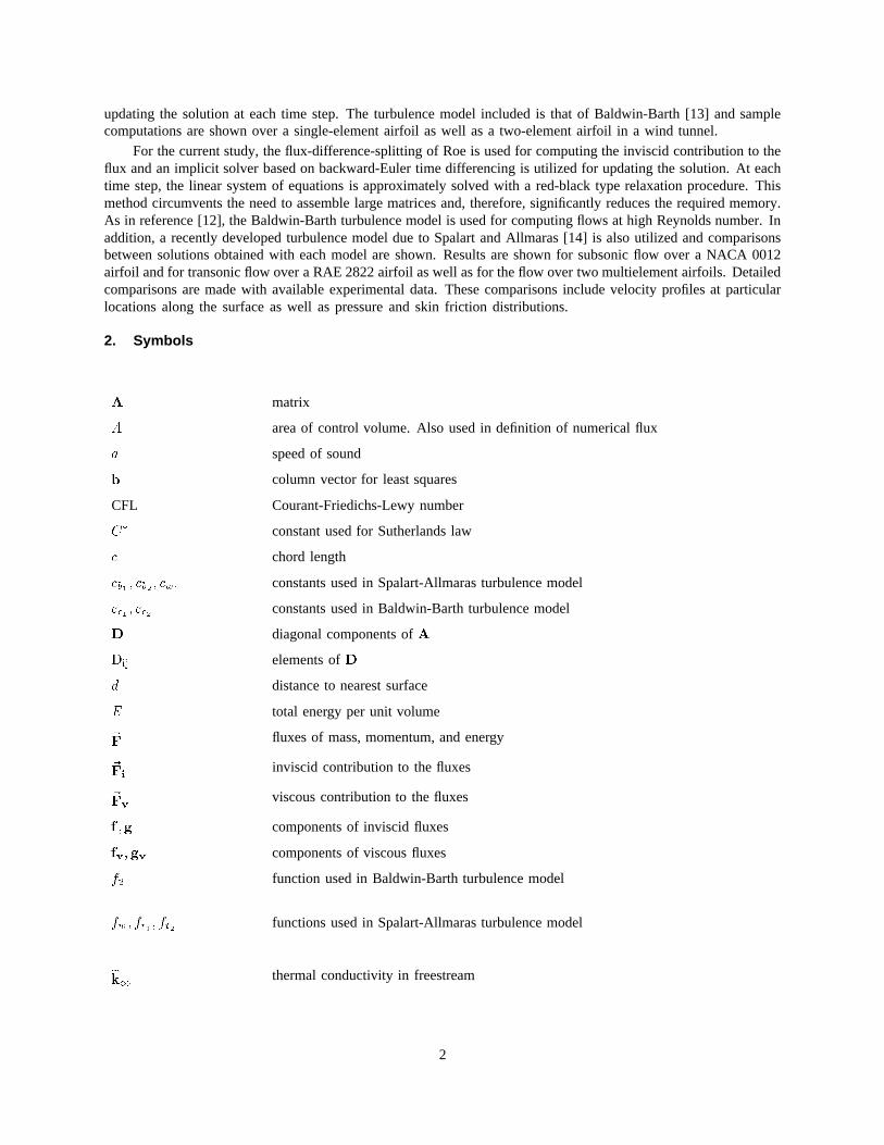
2. Symbols

A matrix

A area of control volume. Also used in definition of numerical flux

a speedof sound

b columnvectorfor leastsquares

CFL Courant-Friedichs-Lewy number

C� constant used for Sutherlands law

c chord length

cb1 ; cb2 ; cw1constantsusedin Spalart-Allmarasturbulencemodel

c�1 ; c�2 constantsusedin Baldwin-Barth turbulence model

D diagonal components ofA

Dij elements ofD

d distanceto nearestsurface

E total energyper unit volume

~F fluxes of mass, momentum, and energy

~Fiinviscid contribution to the fluxes

~Fvviscouscontributionto the fluxes

f ;g componentsof inviscid fluxes

fv;gv components of viscous fluxes

f2 function used in Baldwin-Barth turbulence model

fw; ft1 ; ft2 functions used in Spalart-Allmaras turbulence model

ek1 thermal conductivity in freestream

2

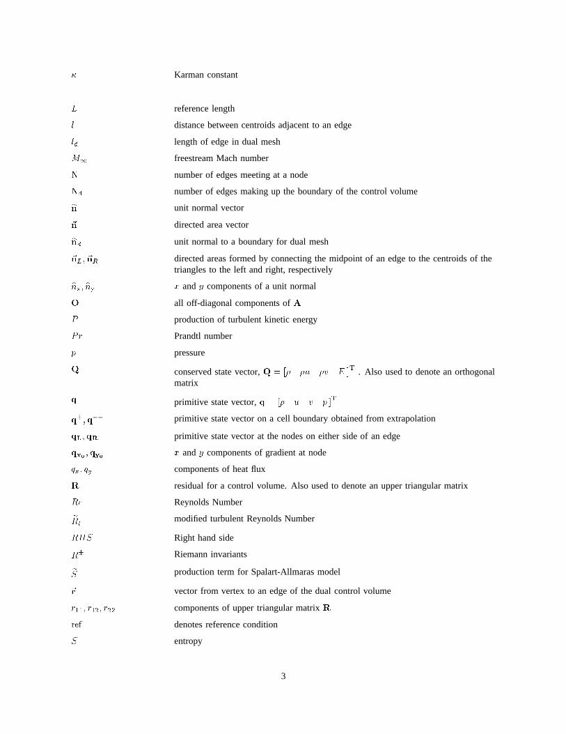
� Karman constant

L reference length

l distance between centroids adjacent to an edge

ld length of edge in dual mesh

M1 freestream Mach number

N number of edges meeting at a node

Nd number of edges making up the boundary of the control volume

bn unit normal vector

~n directed area vector

bnd unit normal to a boundary for dual mesh

~nL; ~nR directedareasformed by connecting the midpoint of an edge to the centroids of thetriangles to the left and right, respectively

bnx; bny x andy components of a unit normal

O all off-diagonalcomponents ofA

P production of turbulent kinetic energy

Pr Prandtlnumber

p pressure

Q conserved state vector,Q = [� �u �v E ]T . Also used to denote an orthogonal

matrix

q primitive statevector,q = [� u v p ]T

q+;q� primitive statevectoron a cell boundary obtained from extrapolation

qL;qR primitive state vector at the nodes on either side of an edge

qx0 ;qy0 x andy components of gradient at node

qx; qy components of heat flux

R residual for a control volume. Also used to denote an upper triangular matrix

Re Reynolds Number

eRtmodified turbulent Reynolds Number

RHS Right hand side

R� Riemann invariants

eS production term for Spalart-Allmaras model

~r vector from vertex to an edge of the dual control volume

r11; r12; r22 components of upper triangular matrixR

ref denotes reference condition

S entropy

3

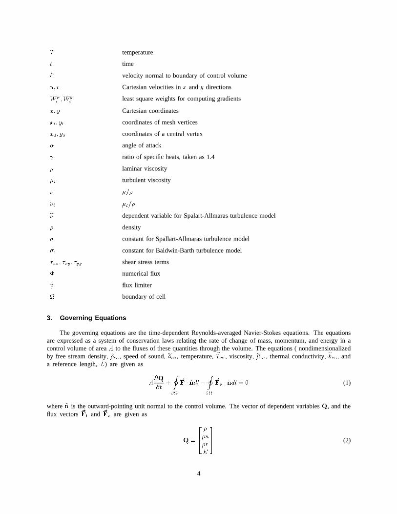
T temperature

t time

U velocity normal to boundary of control volume

u; v Cartesian velocities inx andy directions

W xi ;W

yi

leastsquareweightsfor computinggradients

x; y Cartesian coordinates

xi; yi coordinates of mesh vertices

x0; y0 coordinates of a central vertex

� angleof attack

ratio of specific heats, taken as 1.4

� laminar viscosity

�t turbulent viscosity

� �=�

�t �t=�

e� dependentvariablefor Spalart-Allmaras turbulence model

� density

� constant for Spallart-Allmaras turbulence model

�� constant for Baldwin-Barth turbulence model

�xx; �xy; �yy shearstressterms

� numericalflux

flux limiter

boundary of cell

3. Governing Equations

The governing equations are the time-dependent Reynolds-averaged Navier-Stokes equations. The equationsare expressed as a system of conservation laws relating the rate of change of mass, momentum, and energy in acontrol volume of areaA to the fluxes of these quantities through the volume. The equations ( nondimensionalizedby free streamdensity,e�1, speedof sound,ea1, temperature,eT1, viscosity, e�1, thermalconductivity,ek1, anda referencelength, L) are given as

A@Q

@t+

I@

~F � n̂dl �

I@

~Fv � n̂dl = 0 (1)

wherebn is the outward-pointing unit normal to the control volume. The vector of dependent variablesQ, and theflux vectors~Fi and ~Fv are given as

Q =

264�

�u

�v

E

375 (2)

4

~Fi = f bi + g bj =

264

�u

�u2 + p

�uv

(E + p)u

375bi+

264

�v

�vu

�v2 + p

(E + p)v

375bj (3)

~Fv = fvbi + gvbj =264

0

�xx�xy

u�xx + v�xy � qx

375bi +

264

0

�xy�yy

u�yx + v�yy � qy

375bj (4)

Here,~Fi and~Fv are the inviscid and viscous flux vectors respectively; the shear stress and heat conduction termsare given as

�xx = (�+ �t)M1

Re

2

3[2ux � vy] (5)

�yy = (� + �t)M1

Re

2

3[2vy � ux] (6)

�xy = (� + �t)M1

Re[uy + vx] (7)

qx =�M1

Re( � 1)

��

Pr+

�t

Prt

�@a2

@x(8)

qy =�M1

Re( � 1)

��

Pr+

�t

Prt

�@a2

@y(9)

The equationsare closed with the equation of state for a perfect gas

p = ( � 1)�E � �

�u2 + v2

�=2�

(10)

and the laminar viscosity is determined through Sutherland’s law

�

�1=

(1 + C�)

(T=T1 +C�)(T=T1)

3=2 (11)

whereC� = 198:6

460:0is Sutherland’s constant divided by a free stream reference temperature which is assumed to

be 460� Rankine.

4. Solution Algorithm

The flow solver is an implicit, upwind-differencing algorithm in which the inviscid fluxes are obtained on thefacesof eachcontrol volume using the flux-difference-splittingtechnique of Roe [10]. For the current scheme, anode-based algorithm is used in which the variables are stored at the vertices of the mesh and the equations aresolved on non-overlapping control volumes surrounding each node. The viscous terms are evaluated with a finite-volume formulation which is equivalent to a Galerkin-type approximation and results in a central-difference-typeformulation for these terms. The solution at each time step is updated using the linearized backward-Euler, time-differencing scheme. At each time step, the linear system of equations is approximately solved with a subiterativeprocedure in which the unknowns are divided into two groups (colors) according to whether the node number iseven or odd. For each subiteration, the solution is obtained by solving for all the unknowns in one color beforeproceeding to the next one. This corresponds to a red-black type of iterative algorithm for solving the linear system.

5

4.1. Finite Volume Scheme

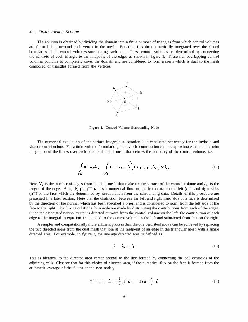
The solution is obtained by dividing the domain into a finite number of triangles from which control volumesare formed that surround each vertex in the mesh. Equation 1 is then numerically integrated over the closedboundaries of the control volumes surrounding each node. These control volumes are determined by connectingthe centroid of each triangle to the midpoint of the edges as shown in figure 1. These non-overlapping controlvolumes combine to completely cover the domain and are considered to form a mesh which is dual to the meshcomposed of triangles formed from the vertices.

24

5

3

1

0

6

Figure 1. Control Volume Surrounding Node

The numericalevaluation of the surface integrals in equation 1 is conducted separately for the inviscid andviscous contributions. For a finite volume formulation, the inviscid contribution can be approximated using midpointintegration of the fluxes over each edge of the dual mesh that defines the boundary of the control volume. i.e.

I@

~F � n̂ddld =

I@

~F � d~nd �

NdXi=1

��q+;q�; bndi

�� ldi (12)

HereNd is the number of edges from the dual mesh that make up the surface of the control volume andldi is thelength of the edge. Also,�(q+;q�; bndi) is a numerical flux formed from data on the left (q+) and right sides(q�) of the face which are determined by extrapolation from the surrounding data. Details of this procedure arepresented in a later section. Note that the distinction between the left and right hand side of a face is determinedby the direction of the normal which has been specified a priori and is considered to point from the left side of thefaceto the right. The flux calculations for a node are made by distributing the contributions from each of the edges.Since the associated normal vector is directed outward from the control volume on the left, the contribution of eachedge to the integral in equation 12 is added to the control volume to the left and subtracted from that on the right.

A simpler and computationally more efficient process than the one described above can be achieved by replacingthe two directedareasfrom the dual meshthat join at the midpoint of an edgein the triangular mesh with a singledirected area. For example, in figure 2, the average directed area is defined as

~n = ~nL + ~nR (13)

This is identical to the directedareavector normal to the line formed by connecting the cell centroids of theadjoining cells. Observe that for this choice of directed area, if the numerical flux on the face is formed from thearithmetic average of the fluxes at the two nodes,

��q+;q�; bn� = 1

2

�~F(qL) + ~F(qR)

�� bn (14)

6

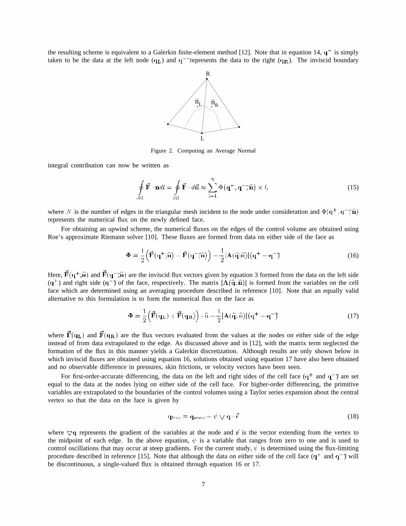
the resulting scheme is equivalent to a Galerkin finite-element method [12]. Note that in equation 14,q+ is simplytaken to be the data at the left node (qL) and q� representsthe data to the right (qR). The inviscid boundary

nL nR

L

R

Figure 2. Computing an Average Normal

integral contribution can now be written as

I@

~F � n̂dl =

I@

~F � d~n �

NXi=1

��q+;q�; bn�� li (15)

whereN is the numberof edgesin the triangular mesh incident to the node under consideration and�(q+;q�; bn)represents the numerical flux on the newly defined face.

For obtaining an upwind scheme, the numerical fluxes on the edges of the control volume are obtained usingRoe’s approximate Riemann solver [10]. These fluxes are formed from data on either side of the face as

� =1

2

�~F�q+;bn�+ ~F

�q�;bn��� 1

2jA(bq;bn)j�q+ � q�� (16)

Here,~F(q+;bn) and~F(q�;bn) are the inviscid flux vectors given by equation 3 formed from the data on the left side(q+) and right side (q�) of the face, respectively. The matrixjA(bq; bn)j is formed from the variables on the cellface which are determined using an averaging procedure described in reference [10]. Note that an equally validalternative to this formulation is to form the numerical flux on the face as

� =1

2

�~F(qL) + ~F(qR)

�� bn� 1

2jA(bq; bn)j�q+ � q�� (17)

where~F(qL) and ~F(qR) are the flux vectorsevaluatedfrom the values at the nodes on either side of the edgeinstead of from data extrapolated to the edge. As discussed above and in [12], with the matrix term neglected theformation of the flux in this manner yields a Galerkin discretization. Although results are only shown below inwhich inviscid fluxes are obtained using equation 16, solutions obtained using equation 17 have also been obtainedand no observabledifferencein pressures,skin frictions, or velocity vectors have been seen.

For first-order-accuratedifferencing,the dataon the left and right sidesof the cell face (q+ andq�) are setequal to the data at the nodes lying on either side of the cell face. For higher-order differencing, the primitivevariables are extrapolated to the boundaries of the control volumes using a Taylor series expansion about the centralvertex so that the data on the face is given by

qface = qnode + 5 q �~r (18)

where5q represents the gradient of the variables at the node and~r is the vector extending from the vertex tothe midpoint of each edge. In the above equation, is a variable that ranges from zero to one and is used tocontrol oscillations that may occur at steep gradients. For the current study, is determined using the flux-limitingprocedure described in reference [15]. Note that although the data on either side of the cell face (q+ andq�) willbe discontinuous, a single-valued flux is obtained through equation 16 or 17.

7

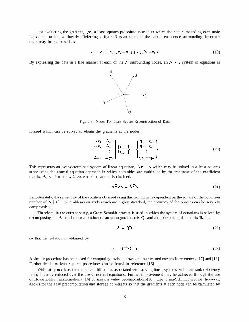
For evaluating the gradient,5q, a least squares procedure is used in which the data surrounding each nodeis assumedto behavelinearly. Referringto figure 3 as an example, the data at each node surrounding the centernode may be expressed as

qi = q0 + qx0(xi � x0) + qy0(yi�y0) (19)

By expressing the data in a like manner at each of theN surrounding nodes, anN � 2 system of equations is

42

1

3

5

0

Figure 3. Nodes For Least Square Reconstruction of Data

formed which can be solved to obtain the gradients at the nodes

2664�x1�x2

...�xN

�y1�y2

...�yN

3775�qx0qy0

�=

8>><>>:

q1 � q0q2 � q0

...qN � q0

9>>=>>;

(20)

This representsan over-determinedsystem of linear equations,Ax = b which may be solved in a least squaressense using the normal equation approach in which both sides are multiplied by the transpose of the coefficientmatrix, A, so that a2 � 2 system of equations is obtained.

ATAx = ATb (21)

Unfortunately, the sensitivity of the solution obtained using this technique is dependent on the square of the conditionnumberof A [16]. For problems on grids which are highly stretched, the accuracy of the process can be severelycompromised.

Therefore,in the current study, a Gram-Schmidt process is used in which the system of equations is solved bydecomposing theA matrix into a product of an orthogonal matrixQ, and an upper triangular matrixR, i.e.

A = QR (22)

so that the solution is obtainedby

x = R�1QTb (23)

A similar procedurehasbeenusedfor computinginviscid flows on unstructuredmeshesin references [17] and [18].Further details of least squares procedures can be found in reference [16].

With this procedure, the numerical difficulties associated with solving linear systems with near rank deficiencyis significantly reduced over the use of normal equations. Further improvement may be achieved through the useof Householder transformations [16] or singular value decompositions[16]. The Gram-Schmidt process, however,allows for the easy precomputation and storage of weights so that the gradients at each node can be calculated by

8

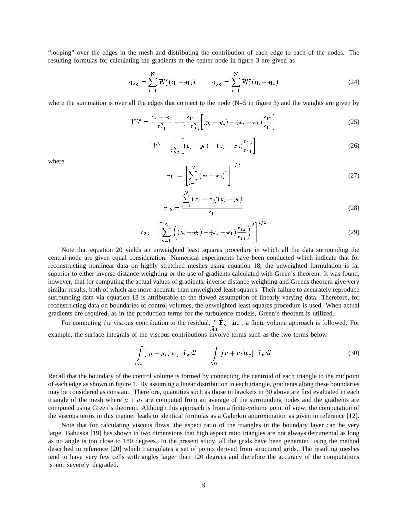
“looping” over the edges in the mesh and distributing the contribution of each edge to each of the nodes. Theresultingformulasfor calculatingthe gradientsat the center node in figure 3 are given as

qx0 =

NXi=1

Wxi (qi � q0) qy0 =

NXi=1

Wyi (qi � q0) (24)

where the summation is over all the edges that connect to the node (N=5 in figure 3) and the weights are given by

W xi =

xi � x0

r211�

r12

r11r222

�(yi � y0) � (xi � x0)

r12

r11

�(25)

Wyi =

1

r222

�(yi � y0) � (xi � x0)

r12

r11

�(26)

where

r11 =

"NXi=1

(xi � x0)2

#1=2(27)

r12 =

NPi=1

(xi � x0)(yi � y0)

r11(28)

r22 =

"NXi=1

�(yi � y0)� (xi � x0)

r12

r11

�2#1=2(29)

Note that equation 20 yields an unweighted least squares procedure in which all the data surrounding thecentralnode are given equal consideration.Numericalexperimentshavebeenconducted which indicate that forreconstructing nonlinear data on highly stretched meshes using equation 18, the unweighted formulation is farsuperior to either inverse distance weighting or the use of gradients calculated with Green’s theorem. It was found,however, that for computing the actual values of gradients, inverse distance weighting and Greens theorem give verysimilar results, both of which are more accurate than unweighted least squares. Their failure to accurately reproducesurrounding data via equation 18 is attributable to the flawed assumption of linearly varying data. Therefore, forreconstructing data on boundaries of control volumes, the unweighted least squares procedure is used. When actualgradients are required, as in the production terms for the turbulence models, Green’s theorem is utilized.

For computing the viscous contribution to the residual,R@

bFv � bndl, a finite volume approach is followed. For

example, the surface integrals of the viscous contributions involve terms such as the two terms belowZ@

[(�+ �t)ux] � bnxdlZ@

[(�+ �t)vy] � bnxdl (30)

Recall that the boundary of the control volume is formed by connecting the centroid of each triangle to the midpointof each edge as shown in figure 1. By assuming a linear distribution in each triangle, gradients along these boundariesmaybeconsideredasconstant.Therefore,quantitiessuch as those in brackets in 30 above are first evaluated in eachtriangle of the mesh where� + �t are computed from an average of the surrounding nodes and the gradients arecomputed using Green’s theorem. Although this approach is from a finite-volume point of view, the computation ofthe viscous terms in this manner leads to identical formulas as a Galerkin approximation as given in reference [12].

Note that for calculating viscous flows, the aspect ratio of the triangles in the boundary layer can be verylarge. Babuska [19] has shown in two dimensions that high aspect ratio triangles are not always detrimental as longas no angle is too close to 180 degrees. In the present study, all the grids have been generated using the methoddescribed in reference [20] which triangulates a set of points derived from structured grids. The resulting meshestend to have very few cells with angles larger than 120 degrees and therefore the accuracy of the computationsis not severely degraded.

9

4.2. Time Advancement Scheme

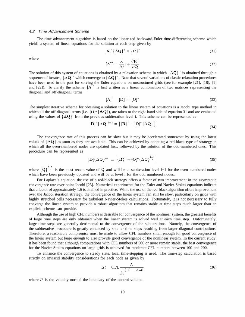
The time advancement algorithm is based on the linearized backward-Euler time-differencing scheme whichyields a system of linear equations for the solution at each step given by

[A]nf�Qgn = fRgn (31)

where

[A]n =A

�tI +

@Rn

@Q(32)

The solutionof this systemof equations is obtained by a relaxation scheme in whichf�Qgn is obtainedthrougha

sequenceof iterates,f�Qgi which convergeto f�Qgn. Notethatseveralvariationsof classic relaxation procedureshave been used in the past for solving the Euler equations on unstructured grids (see for example [21], [18], [1]and [22]). To clarify the scheme,[A]n is first written as a linear combination of two matrices representing thediagonal and off-diagonal terms

[A]n = [D]n + [O]n (33)

The simplestiterativescheme for obtaining a solution to the linear system of equations is a Jacobi type method inwhich all the off-diagonal terms (i.e.[O]nf�Qg), are taken to the right-hand side of equation 31 and are evaluatedusing the values off�Qgi from the previous subiteration level i. This scheme can be represented as

[D]nf�Qgi+1 =�fRgn � [O]nf�Qgi

�(34)

The convergencerate of this processcan be slow but it may be accelerated somewhat by using the latestvalues off�Qg as soon as they are available. This can be achieved by adopting a red-black type of strategy inwhich all the even-numberednodesare updatedfirst, followed by the solution of the odd-numberedones. Thisprocedure can be represented as

[D]f�Qgi+1 =hfRgn � [O]nf�Qg

i+1

i

i(35)

wherefQgi+1

i is the most recent value ofQ and will be at subiteration level i+1 for the even numbered nodeswhich have been previously updated and will be at level i for the odd numbered nodes.

For Laplace’s equation, the use of a red-black strategy offers a factor of two improvement in the asymptoticconvergence rate over point Jacobi [23]. Numerical experiments for the Euler and Navier-Stokes equations indicatethata factorof approximately 1.6 is attained in practice. While the use of the red-black algorithm offers improvementover the Jacobi iteration strategy, the convergence of the linear system can still be slow, particularly on grids withhighly stretched cells necessary for turbulent Navier-Stokes calculations. Fortunately, it is not necessary to fullyconverge the linear system to provide a robust algorithm that remains stable at time steps much larger than anexplicit scheme can provide.

Althoughthe use of high CFL numbers is desirable for convergence of the nonlinear system, the greatest benefitsof large time stepsare only obtainedwhen the linear system is solved well at each time step. Unfortunately,large time stepsare generallydetrimentalto the convergence of the subiterations. Namely, the convergence ofthe subiterative procedure is greatly enhanced by smaller time steps resulting from larger diagonal contributions.Therefore, a reasonable compromise must be made to allow CFL numbers small enough for good convergence ofthe linear system but large enough to also provide good convergence of the nonlinear system. In the current study,it has been found that although computations with CFL numbers of 500 or more remain stable, the best convergencefor the Navier-Stokesequationson largegrids is achieved for moderate CFL numbers between 100 and 200.

To enhance the convergence to steady state, local time-stepping is used. The time-step calculation is basedstrictly on inviscid stability considerations for each node as given by

�t = CFLAR

@

(jUj+ a)d l(36)

whereU is the velocity normal the boundary of the control volume.

10

4.3. Boundary Conditions

The boundary conditions on the body correspond to no-slip and a prescribed wall temperature. They areenforced by modifying the matrix terms in equation 35 to appropriately reflect the desired boundary conditions.To more clearly demonstrate the procedure, a slightly expanded representation of one of the rows in equation 35is given by

264D11 D12 D13 D14

D21 D22 D23 D24

D31 D32 D33 D34

D41 D42 D43 D44

375

8><>:

����u��v�E

9>=>;

=

8><>:

RHS1RHS2RHS3RHS4

9>=>;

(37)

whereRHS represents both the residual and off-diagonal terms on the right hand side of equation 35 andDij

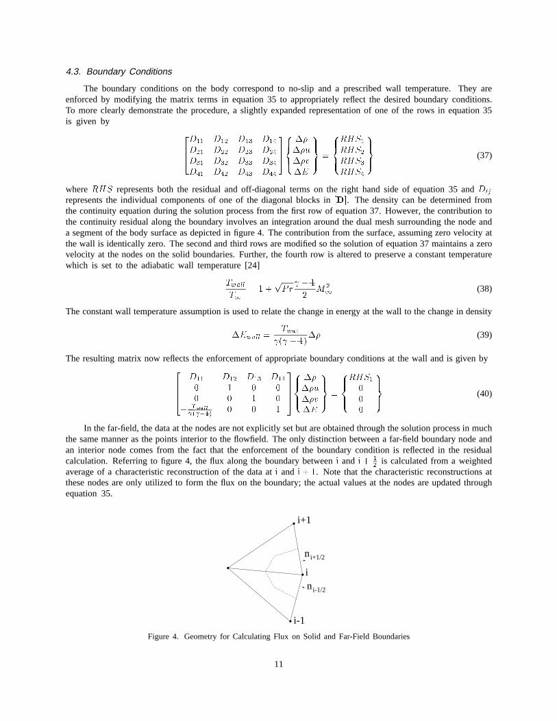
representsthe individual componentsof one of the diagonal blocks in[D]. The densitycan be determinedfromthe continuity equation during the solution process from the first row of equation 37. However, the contribution tothe continuity residual along the boundary involves an integration around the dual mesh surrounding the node anda segment of the body surface as depicted in figure 4. The contribution from the surface, assuming zero velocity atthe wall is identically zero. The second and third rows are modified so the solution of equation 37 maintains a zerovelocity at the nodes on the solid boundaries. Further, the fourth row is altered to preserve a constant temperaturewhich is set to the adiabatic wall temperature [24]

Twall

T1

= 1 +pPr

� 1

2M2

1(38)

The constantwall temperatureassumptionis used to relate the change in energy at the wall to the change in density

�Ewall =Twall

( � 1)�� (39)

The resulting matrix now reflects the enforcement of appropriate boundary conditions at the wall and is given by2664

D11 D12 D13 D14

0 1 0 00 0 1 0

� Twall ( �1)

0 0 1

3775

8><>:

����u��v�E

9>=>;

=

8><>:

RHS1000

9>=>;

(40)

In the far-field, the data at the nodes are not explicitly set but are obtained through the solution process in muchthe same manner as the points interior to the flowfield. The only distinction between a far-field boundary node andan interior node comes from the fact that the enforcement of the boundary condition is reflected in the residualcalculation. Referring to figure 4, the flux along the boundary betweeni and i + 1

2is calculated from a weighted

average of a characteristic reconstruction of the data ati and i + 1. Note that the characteristic reconstructions atthese nodes are only utilized to form the flux on the boundary; the actual values at the nodes are updated throughequation 35.

ni+1/2

i+1

i

i-1

ni-1/2

Figure 4. Geometry for Calculating Flux on Solid and Far-Field Boundaries

11

For obtaining the characteristic reconstruction in the far-field, the flow-field is assumed to be essentially inviscidso that quantitiesneededfor the computation of the flux along the outer boundary are obtained from two locallyone-dimensional Riemann invariants. While this assumption is not strictly valid, the perturbations from inviscid floware generally small so that the assumption of inviscid flow is acceptable. The Riemann invariants are consideredconstant along characteristics defined normal to the outer boundary and are given as

R� = U �2a

� 1(41)

For subsonicflow, R� canbe evaluatedlocally from free stream conditions taken to be outside the computationaldomain andR+ is evaluatedlocally from the interior of the domain and is taken to correspond to the present valueof the data at each node on the outer boundary. The local normal velocity and speed of sound on the boundaryare calculated using the Riemann invariants as

Uboundary =1

2

�R++ R

��

(42)

aboundary = � 1

4

�R+ �R

��

(43)

The Cartesian velocities are determined on the outer boundary by decomposing the normal and tangentialvelocity vectors into components yielding

uboundary = uref + bnx(Uboundary �Uref )

vboundary = vref + bny(Uboundary �Uref )(44)

where the subscript,ref, representsvaluesobtained from free stream values for inflow and from current data atthe boundary node for outflow.

The entropyis determinedusingeither the free streamvalueor the value at the boundary node depending onwhether the boundary is an inflow or outflow boundary. Once the entropy is known, the density on the far-fieldboundary is calculated from the entropy and speed of sound as

�boundary =

a2boundary

Sboundary

! 1

�1

(45)

The energy is then calculated from the equation of state and the flux is then calculated using these characteristicreconstructions.

4.4. Turbulence Modeling

For the current study, two different turbulence models are considered. At each time step, the equation forthe turbulent viscosity is solved separately from the flow equations resulting in a loosely coupled solution processthat allows for the easy interchange of new turbulence models. The turbulence models considered in the currentstudy are that of Baldwin and Barth [13] and Spalart and Allmaras [14]. The governing equation for each of thesemodels is given below although reference to the original publications should be made for the precise meaning ofall the terms and for details related to the implementation.

The first model is that of Baldwin and Barth, which is a one-equation advection-diffusion model derived usingthek�� equations. The dependent variable for the model is a field quantity ,� eRt, from which the turbulent viscositycan be obtained from an algebraic relation. The partial differential equation for� eRt is given in non-dimensionalterms as

D�� eRt

�Dt

=M1

Re

��� +

2�t

��

�52�� eRt

��

1

��

r ���tr

�� eRt

���

+ (c�2f2 � c�1)

q� eRtP

(46)

12

Here, the left hand side of the equation is the substantial derivative

D(�)

Dt=

@(�)

@t+ u

@(�)

@x+ v

@(�)

@y(47)

and the right hand side of the equation represents diffusion and production terms respectively. The details of eachof the terms can be found in reference [13].

In addition to the turbulencemodel of Baldwin and Barth, the model of Spalart and Allmaras [14] has alsobeen utilized. This is also a one–equation turbulence model but its derivation is much more heuristic in nature,relying heavily on empiricism and dimensional analysis. The form of this equation is similar to that of the previousmodel and is given by

D(e�)Dt

= cb1 [1� ft2 ]eSe� + M

1

�Re

�r �

�(� + (1 + cb2)e�)re� � cb2e�r2e���

�M1

Re

hcw1

fw �cb1

�2ft2

i�e�d

�2+

Re

M1

ft1�U2

(48)

where again, the original reference should be consulted for a precise explanation of each of the terms. Note however,that this model includes a destruction term which is absent in the previous model as well as a source term usedfor specifying transition locations.

For both the Baldwin-Barth and the Spalart-Allmaras turbulence models, the equations are solved using abackward-Euler time-stepping-scheme similar to that used for the flow variables. For both models, the dependentvariable(� eRt for Baldwin-Barthande� for Spalart-Allmaras) is specified to be zero on the body and is thereforenot solved for during the solution process. In the far-field, the dependent variable is taken to be free stream forinflow and is extrapolated from the interior for outflow. For the discretization of the terms in each model, theconvectivetermsareevaluatedwith first-orderupwind differencingand the higher-orderderivativesareevaluatedin the same manner as described for the flow solver.

5. Numerical Results

Resultsare shown below for severaltest cases. For each case, the CFL number has been linearly rampedfrom 20 to 100 over 100 iterations and 15 subiterations were done at each time step to obtain an approximatesolution of the linear system. While this strategy is in no way optimal for every case, it has been found to yieldsatisfactory results. As previously mentioned, all the grids used in the current study have been generated withthe code described in reference [20] which triangulates point sets derived from structured grids generated aroundindividual components. Consequently, few large angles appear in the mesh; typically fewer than two percent ofthe angles are larger than 120 degrees.

All the figures shown below have been obtained assuming fully turbulent flow by specifying a small level ofturbulent viscosity in the free stream. Although not shown, studies with the Spalart-Allmaras turbulence model tospecifytransitionlocations and to examine the effects of varying the level of free stream turbulence have also beenconducted. For the cases considered, neither effect yielded major differences in the flowfields.

5.1. NACA 0012 Airfoil

The first test caseis flow over the NACA airfoil at a free stream Mach number of 0.7, an angle of attackof 1.49 degrees, and a Reynolds number of 9.0 million. Computations for this case have been computed using awide range of codes with a compilation of results being reported in reference [25]. The grid used for the presentcomputations consists of 28,126 nodes, of which 202 lie on the airfoil surface. The average normal spacing atthe wall for this grid is2 � 10�6.

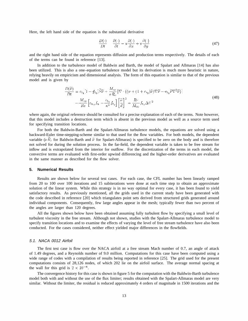
The convergence history for this case is shown in figure 5 for the computation with the Baldwin-Barth turbulencemodel both with and without the use of the flux limiter; results obtained with the Spalart-Allmaras model are verysimilar. Without the limiter, the residual is reduced approximately 4 orders of magnitude in 1500 iterations and the

13

final lift is obtained in less than 700 iterations. With the use of the limiter, the residual is reduced only one andone-halfordersof magnitudebefore enteringinto a limit cycle oscillation. The lift, however, exhibits the sameconvergence behavior as when the limiter is not used.

Figure 5. ConvergenceHistory for NACA 0012

Since the flux limiter used in the present calculations is non-differentiable and is sensitive to perturbationson the order of truncation error [26], its use yields residuals which are typically reduced only one or two ordersof magnitude before entering into a limit cycle oscillation. For cases in which the limiter is used, convergence isdetermined primarily by monitoring the lift coefficient and other physical parameters such as velocity profiles andskin frictions. While alternateflux limiters existsfor structuredgrids which lessenthis tendency, further work isrequired to extend their use for unstructured grids. Most limiters developed for structured grids limit gradients ina one-dimensionalfashion,limiting the gradientsnormal to a cell face independentlyin eachdirection. The taskof reconstructingdataon cell facesfor the currentwork is currently handled in a more “multidimensional” fashionin which a single gradient for each variable is calculated from adjoining data and is used for extrapolating data toeach of the boundaries of the control volume.

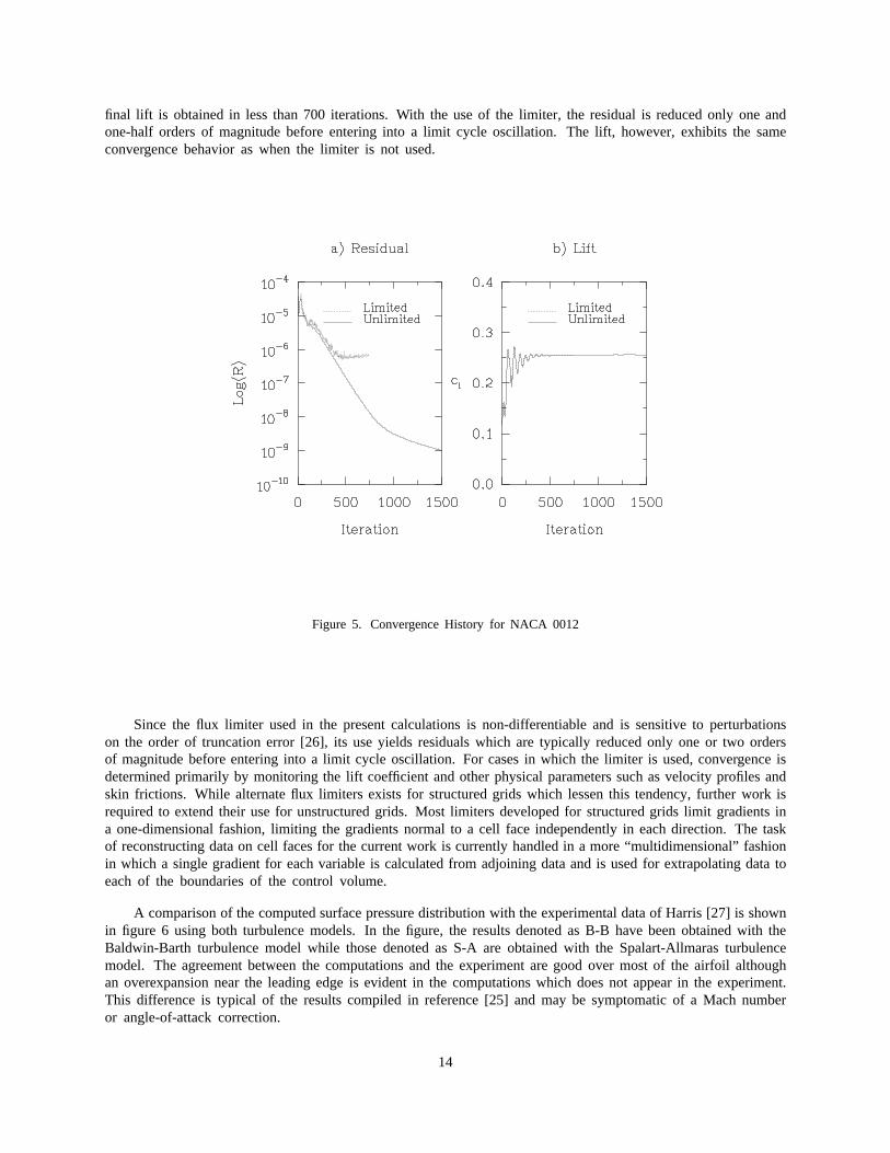
A comparison of the computed surface pressure distribution with the experimental data of Harris [27] is shownin figure 6 using both turbulence models. In the figure, the results denoted as B-B have been obtained with theBaldwin-Barth turbulence model while those denoted as S-A are obtained with the Spalart-Allmaras turbulencemodel. The agreement between the computations and the experiment are good over most of the airfoil althoughan overexpansion near the leading edge is evident in the computations which does not appear in the experiment.This difference is typical of the results compiled in reference [25] and may be symptomatic of a Mach numberor angle-of-attack correction.

14

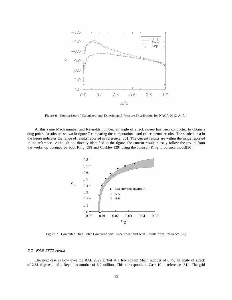
Figure 6. Comparison of Calculated and Experimental Pressure Distribution for NACA 0012 Airfoil

At this sameMach numberand Reynolds number, an angle of attack sweep has been conducted to obtain adrag polar. Results are shown in figure 7 comparing the computational and experimental results. The shaded area inthe figure indicates the range of results reported in reference [25]. The current results are within the range reportedin the reference. Although not directly identified in the figure, the current results closely follow the results fromthe workshop obtained by both King [28] and Coakley [29] using the Johnson-King turbulence model[30].

EXPERIMENT (HARRIS)

0.00 0.01 0.02 0.03 0.04 0.050.0

0.1

0.2

0.3

0.4

0.5

0.6

0.7

0.8

CD

CL

S-A

B-B

Figure 7. Computed Drag Polar Compared with Experiment and with Results from Reference [25]

5.2. RAE 2822 Airfoil

The next case is flow over the RAE 2822 airfoil at a free stream Mach number of 0.75, an angle of attackof 2.81 degrees, and a Reynolds number of 6.2 million. This corresponds to Case 10 in reference [31]. The grid

15

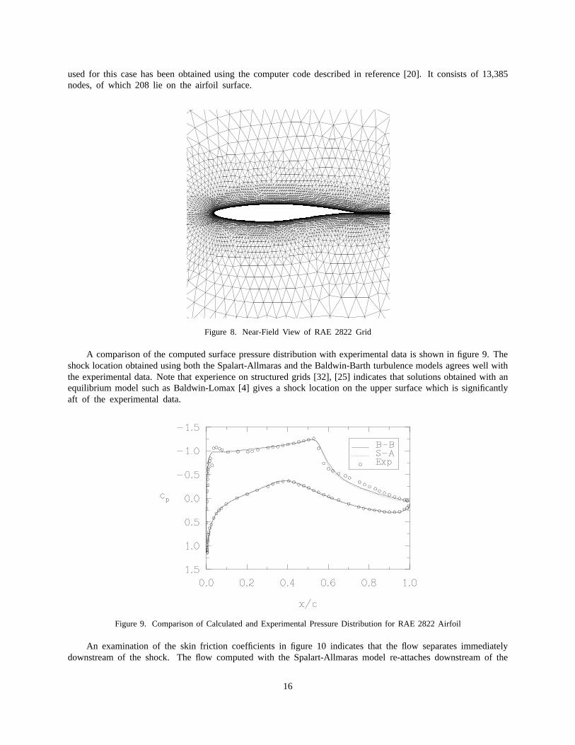
used for this case has been obtained using the computer code described in reference [20]. It consists of 13,385nodes,of which 208 lie on the airfoil surface.

Figure 8. Near-FieldView of RAE 2822 Grid

A comparisonof the computed surface pressure distribution with experimental data is shown in figure 9. Theshock location obtained using both the Spalart-Allmaras and the Baldwin-Barth turbulence models agrees well withthe experimental data. Note that experience on structured grids [32], [25] indicates that solutions obtained with anequilibrium model such as Baldwin-Lomax [4] gives a shock location on the upper surface which is significantlyaft of the experimental data.

Figure 9. Comparison of Calculated and Experimental Pressure Distribution for RAE 2822 Airfoil

An examination of the skin friction coefficients in figure 10 indicates that the flow separates immediatelydownstream of the shock. The flow computed with the Spalart-Allmaras model re-attaches downstream of the

16

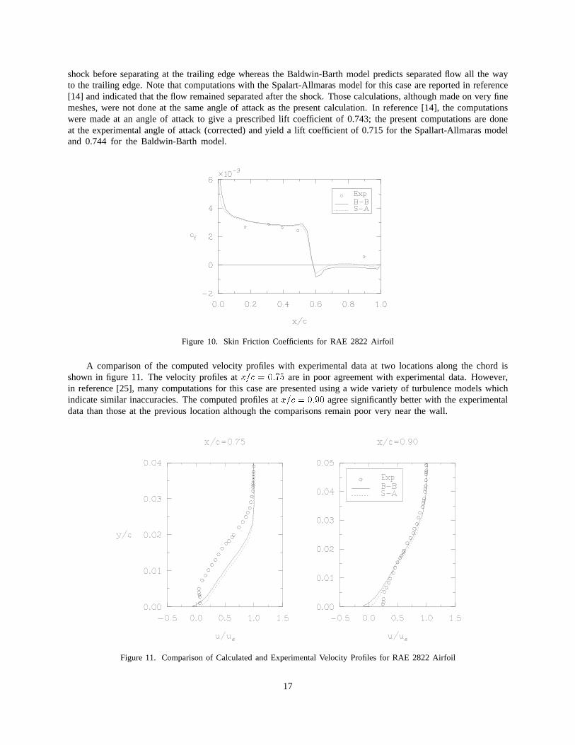
shock before separating at the trailing edge whereas the Baldwin-Barth model predicts separated flow all the wayto the trailing edge.Note that computations with the Spalart-Allmaras model for this case are reported in reference[14] and indicated that the flow remained separated after the shock. Those calculations, although made on very finemeshes, were not done at the same angle of attack as the present calculation. In reference [14], the computationswere made at an angle of attack to give a prescribed lift coefficient of 0.743; the present computations are doneat the experimental angle of attack (corrected) and yield a lift coefficient of 0.715 for the Spallart-Allmaras modeland 0.744 for the Baldwin-Barth model.

Figure 10. Skin Friction Coefficients for RAE 2822 Airfoil

A comparison of the computed velocity profiles with experimental data at two locations along the chord isshownin figure 11. The velocity profilesat x=c = 0:75 are in poor agreementwith experimentaldata. However,in reference [25], many computations for this case are presented using a wide variety of turbulence models whichindicate similar inaccuracies. The computed profiles atx=c = 0:90 agreesignificantlybetterwith the experimentaldatathan those at the previous location although the comparisons remain poor very near the wall.

Figure 11. Comparison of Calculated and Experimental Velocity Profiles for RAE 2822 Airfoil

17

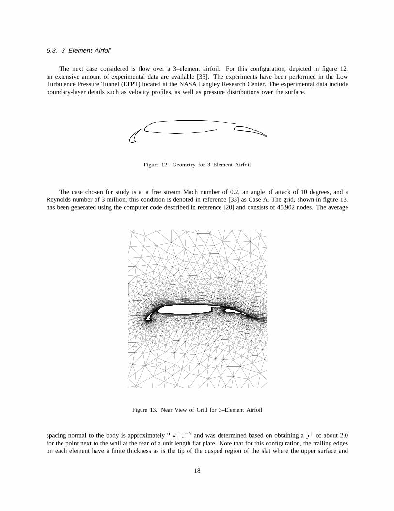
5.3. 3–Element Airfoil

The next caseconsideredis flow over a 3–element airfoil. For this configuration, depicted in figure 12,an extensive amount of experimental data are available [33]. The experiments have been performed in the LowTurbulence Pressure Tunnel (LTPT) located at the NASA Langley Research Center. The experimental data includeboundary-layer details such as velocity profiles, as well as pressure distributions over the surface.

Figure 12. Geometry for 3–Element Airfoil

The case chosen for study is at a free stream Mach number of 0.2, an angle of attack of 10 degrees, and aReynolds number of 3 million; this condition is denoted in reference [33] as Case A. The grid, shown in figure 13,has been generated using the computer code described in reference [20] and consists of 45,902 nodes. The average

Figure 13. Near View of Grid for 3–Element Airfoil

spacing normal to the body is approximately2 � 10�5 and was determined based on obtaining ay

+ of about 2.0for the point next to the wall at the rear of a unit length flat plate. Note that for this configuration, the trailing edgeson each element have a finite thickness as is the tip of the cusped region of the slat where the upper surface and

18

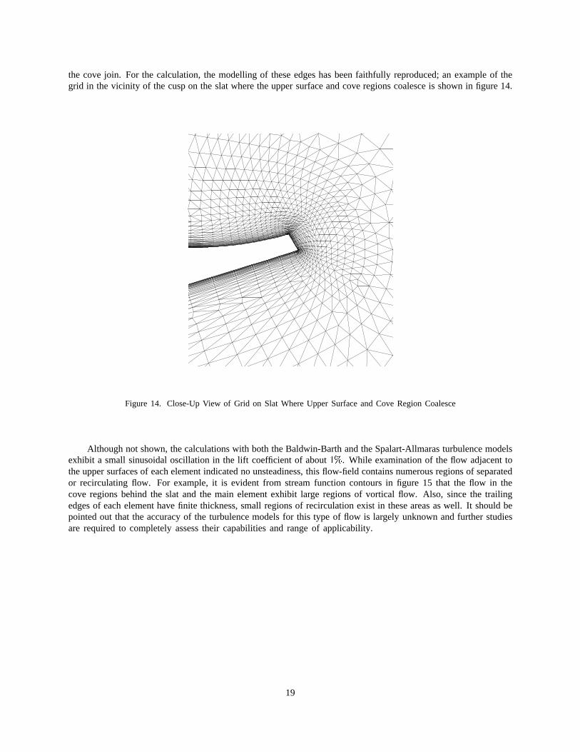
the cove join. For the calculation, the modelling of these edges has been faithfully reproduced; an example of thegrid in the vicinity of the cusp on the slat where the upper surface and cove regions coalesce is shown in figure 14.

Figure 14. Close-Up View of Grid on Slat Where Upper Surface and Cove Region Coalesce

Although not shown, the calculations with both the Baldwin-Barth and the Spalart-Allmaras turbulence modelsexhibit a small sinusoidal oscillation in the lift coefficient of about1%. While examination of the flow adjacent tothe upper surfaces of each element indicated no unsteadiness, this flow-field contains numerous regions of separatedor recirculating flow. For example, it is evident from stream function contours in figure 15 that the flow in thecove regions behind the slat and the main element exhibit large regions of vortical flow. Also, since the trailingedges of each element have finite thickness, small regions of recirculation exist in these areas as well. It should bepointedout that the accuracyof the turbulencemodelsfor this type of flow is largely unknown and further studiesare required to completely assess their capabilities and range of applicability.

19

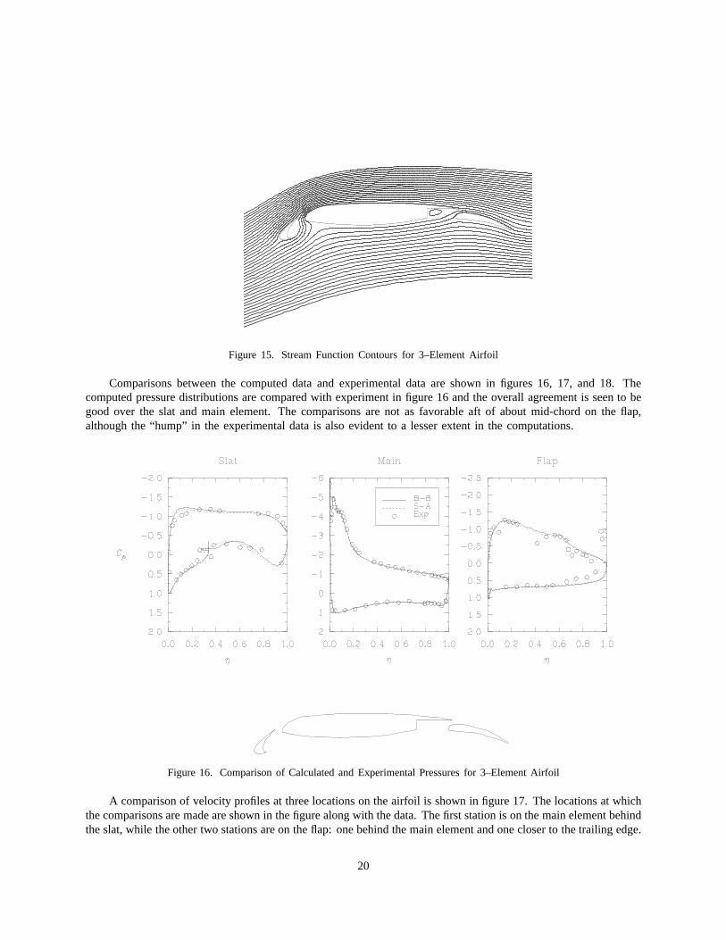
Figure 15. Stream Function Contours for 3–Element Airfoil

Comparisons between the computed data and experimental data are shown in figures 16, 17, and 18. Thecomputedpressuredistributionsarecomparedwith experimentin figure 16 and the overall agreement is seen to begood over the slat and main element. The comparisons are not as favorable aft of about mid-chord on the flap,although the “hump” in the experimental data is also evident to a lesser extent in the computations.

Figure 16. Comparison of Calculated and Experimental Pressures for 3–Element Airfoil

A comparison of velocity profiles at three locations on the airfoil is shown in figure 17. The locations at whichthe comparisons are made are shown in the figure along with the data. The first station is on the main element behindthe slat, while the other two stations are on the flap: one behind the main element and one closer to the trailing edge.

20

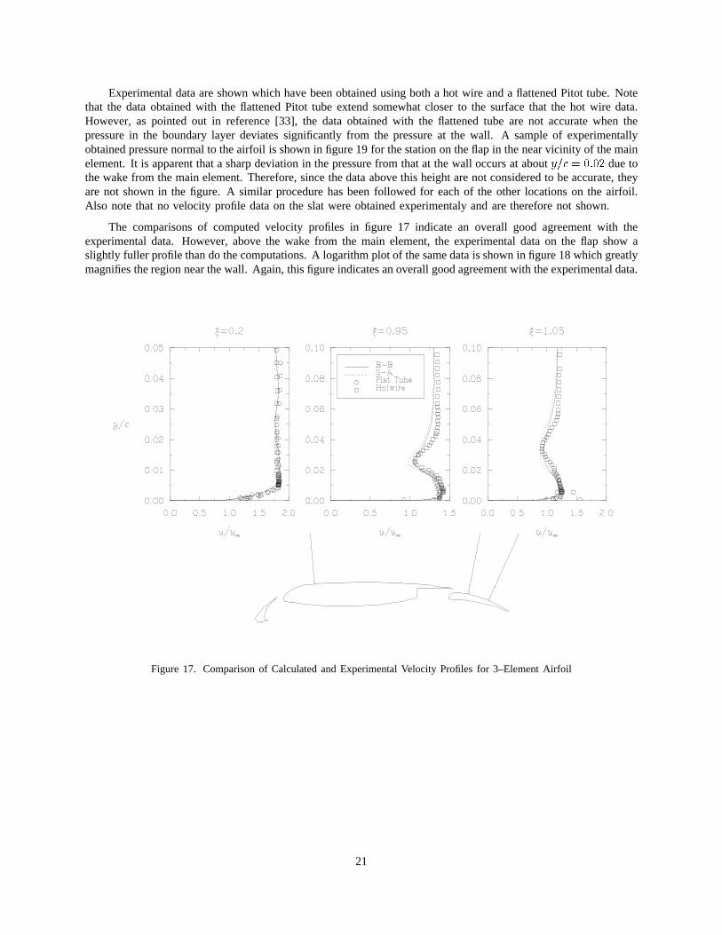
Experimental data are shown which have been obtained using both a hot wire and a flattened Pitot tube. Notethat the data obtainedwith the flattened Pitot tube extend somewhat closer to the surface that the hot wire data.However, as pointed out in reference [33], the data obtained with the flattened tube are not accurate when thepressure in the boundary layer deviates significantly from the pressure at the wall. A sample of experimentallyobtained pressure normal to the airfoil is shown in figure 19 for the station on the flap in the near vicinity of the mainelement. It is apparent that a sharp deviation in the pressure from that at the wall occurs at abouty=c = 0:02 duetothe wake from the main element. Therefore, since the data above this height are not considered to be accurate, theyare not shown in the figure. A similar procedure has been followed for each of the other locations on the airfoil.Also note that no velocity profile data on the slat were obtained experimentaly and are therefore not shown.

The comparisons of computed velocity profiles in figure 17 indicate an overall good agreement with theexperimental data. However, above the wake from the main element, the experimental data on the flap show aslightly fuller profile than do the computations. A logarithm plot of the same data is shown in figure 18 which greatlymagnifies the region near the wall. Again, this figure indicates an overall good agreement with the experimental data.

Figure 17. Comparisonof Calculatedand ExperimentalVelocity Profiles for 3–Element Airfoil

21

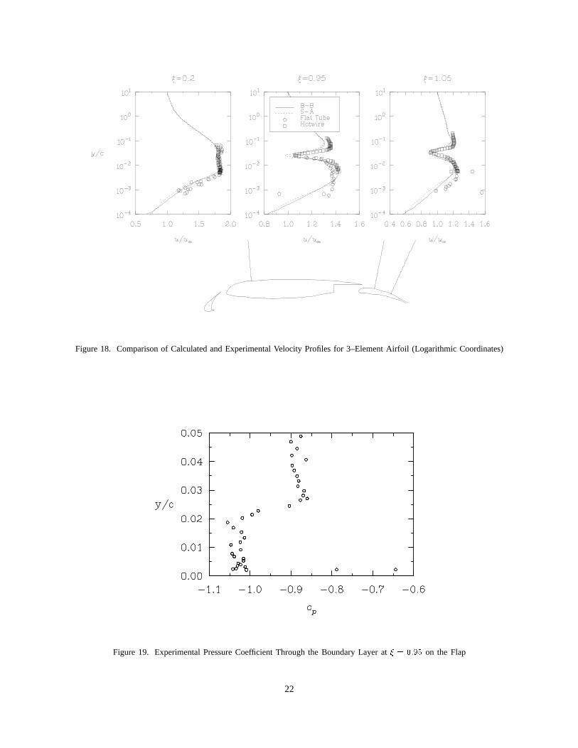
Figure 18. Comparison of Calculated and Experimental Velocity Profiles for 3–Element Airfoil (Logarithmic Coordinates)

Figure 19. Experimental Pressure Coefficient Through the Boundary Layer at� = 0:95 on the Flap

22

5.4. 4–Element Airfoil

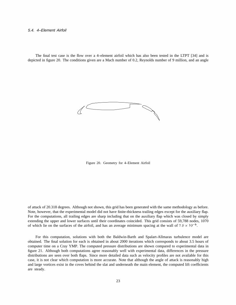
The final test case is the flow over a 4–element airfoil which has also been tested in the LTPT [34] and isdepicted in figure 20. The conditions given are a Mach number of 0.2, Reynolds number of 9 million, and an angle

Figure 20. Geometry for 4–Element Airfoil

of attack of 20.318 degrees. Although not shown, this grid has been generated with the same methodology as before.Note,however,that the experimentalmodeldid not have finite-thickness trailing edges except for the auxiliary flap.For the computations, all trailing edges are sharp including that on the auxiliary flap which was closed by simplyextending the upper and lower surfaces until their coordinates coincided. This grid consists of 59,788 nodes, 1070of which lie on the surfaces of the airfoil, and has an average minimum spacing at the wall of2:0� 10

�5.

For this computation, solutions with both the Baldwin-Barth and Spalart-Allmaras turbulence model areobtained. The final solution for each is obtained in about 2000 iterations which corresponds to about 3.5 hours ofcomputer time on a Cray YMP. The computed pressure distributions are shown compared to experimental data infigure 21. Although both computations agree reasonably well with experimental data, differences in the pressuredistributions are seen over both flaps. Since more detailed data such as velocity profiles are not available for thiscase, it is not clear which computation is more accurate. Note that although the angle of attack is reasonably highand large vortices exist in the coves behind the slat and underneath the main element, the computed lift coefficientsare steady.

23

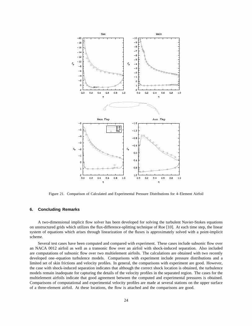
Figure 21. Comparison of Calculated and Experimental Pressure Distributions for 4–Element Airfoil

6. Concluding Remarks

A two-dimensional implicit flow solver has been developed for solving the turbulent Navier-Stokes equationson unstructuredgridswhich utilizes theflux-difference-splittingtechniqueof Roe[10]. At each time step, the linearsystemof equationswhich arisesthroughlinearization of the fluxes is approximately solved with a point-implicitscheme.

Severaltest cases have been computed and compared with experiment. These cases include subsonic flow overan NACA 0012 airfoil as well as a transonic flow over an airfoil with shock-induced separation. Also includedare computations of subsonic flow over two multielement airfoils. The calculations are obtained with two recentlydeveloped one–equation turbulence models. Comparisons with experiment include pressure distributions and alimited set of skin frictions and velocity profiles. In general, the comparisons with experiment are good. However,the case with shock-induced separation indicates that although the correct shock location is obtained, the turbulencemodels remain inadequate for capturing the details of the velocity profiles in the separated region. The cases for themultielementairfoils indicate that good agreement between the computed and experimental pressures is obtained.Comparisons of computational and experimental velocity profiles are made at several stations on the upper surfaceof a three-element airfoil. At these locations, the flow is attached and the comparisons are good.

24

7. Acknowledgments

The authorswould like to acknowledgeTimothy J. Barth of NASA Ames Research Center, Christopher L.Rumsey, Jerry C. South and James L. Thomas of NASA Langley Research Center for many useful conversationspertaining to the present work.

References

1. Karman, S. L.,Development of a 3D Unstructured CFD Method. PhD thesis, The University of Texas atArlington, 1991.

2. Marcum, D. L., and Agarwal, R., “A Three-Dimensional Finite Element Navier-Stokes Solver with k-�

Turbulence Model for Unstructured Grids,”AIAA 90–1652, 1990.

3. Mavriplis, D. J., “Turbulent Flow Calculation Using Unstructured and Adaptive Meshes,”International Journalfor Num. Meth. in Fluids, vol. 13, pp. 1131–1152, 1991.

4. Baldwin, B. S., and Lomax, H., “Thin Layer Approximation and Algebraic Model for Separated TurbulentFlows,” AIAA paper 78–257, 1978.

5. Mavriplis, D. J., and Martinelli, L., “Multigrid Solution of CompressibleTurbulent Flow on UnstructuredMeshes Using a Two-Equation Model,” Tech. Rep. 91–11, ICASE, 1991.

6. Venkatakrishnan,V., and Mavriplis, D. J., “Implicit Solvers for Unstructured Meshes,”AIAA 91–1537CP, 1991.

7. Saad,Y., andSchultz, M. H., “GMRES: A Generalized Minimum Residual Algorithm for Solving NonsymetricLinear Systems,”SIAM J. Sci. Stat.Comp., vol. 7, no. 3, pp. 856–869,1986.

8. Bonhaus,D. L., and Wornom, S. F., “Relative Efficiency and Accuracy of Two Navier-Stokes Codes forSimulating Attach Transonic Flow Over Wings,” Tech. Rep. TP 3061, NASA, 1991.

9. Jou, W., Wigton, L. B., Allmaras, S. R., Spalart, P. R., and Yu, N. J., “Towards Industrial-Strength Navier-Stokes Codes,”Paper Presented at the Fifth Symposium on Numerical and Physical Aspects of AerodynamicFlows, Jan. 1992. Long Beach California.

10. Roe, P., “Approximate Riemann Solvers, Parameter Vectors, and Difference Schemes,”J. of Comp. Phys.,vol. 43, pp. 357–372, 1981.

11. van Leer, B., Thomas, J., Roe, P., and Newsome, R., “A Comparison of Numerical Flux Formulas for theEuler and Navier-Stokes Equations,”AIAA 87–1104, 1987.

12. Barth, T. J., “Numerical Aspects of Computing Viscous High Reynolds Number Flows on UnstructuredMeshes,”AIAA 91–0721, 1991.

13. Baldwin, B. S., and Barth, T. J., “A One-Equation Turbulence Transport Model for High Reynolds NumberWall Bounded Flows,”NASA Technical Memorandum 102847, Aug. 1991.

14. Spalart, P. R., and Allmaras, S. R., “A One-Equation Turbulence Model for Aerodynamic Flows,”AIAA92–0439, 1991.

15. Barth, T., and Jespersen,D., “The Design and Application of Upwind Schemes on Unstructured Meshes,”AIAA 89–0366, 1989.

16. Golub, G., andVAN LOAN , C., Matrix Computations. The Johns Hopkins University Press, 1991.

17. Barth, T. J., “A 3–D Upwind Euler Solver for Unstructured Meshes,”AIAA 91–1548CP, 1991.

18. Anderson,W. K., “Grid Generation and Flow Solution Method for Euler Equations on Unstructured Grids,”Tech. Rep. TM 4295, NASA, 1992.

19. Babuska, I., and Aziz, A. K., “On the Angle Condition in the Finite Element Method,”SIAM J. Numer. Anal.,vol. 13, pp. 214–226, Apr. 1976.

20. Mavriplis, D., “Adaptive Mesh Generation for Viscous Flows using Delaunay Triangulation,”J. of Comp.Phys., vol. 90, pp. 271–291, 1990.

25

21. Batina, J. T., “Implicit Flux-Split Euler Schemes for Unsteady Aerodynamic Analysis Involving UnstructuredDynamic Meshes,”AIAA 90–0936, Apr. 1990.

22. Whitaker, D. L., “Solution Algorithms for the Two-Dimensional Euler Equations on Unstructured Meshes,”AIAA 90–0697, 1990.

23. Hageman, L. A., and Young, D. M.,Applied Iterative Methods. Academic Press, 1981.

24. White, F. M.,Viscous Fluid Flow. McGraw-Hill Book Company, 1974.

25. Holst, T., “Viscous TransonicAirfoil WorkshopCompendiumof Results,”AIAA 87–1460, 1987.

26. Anderson,W. K., Thomas,J. L., and van Leer, B., “A Comparison of Finite Volume Flux Vector Splittingsfor the Euler Equations,”AIAA Journal, vol. 24, pp. 1453–1460, Sept. 1986.

27. Harris, C., “Two-DimensionalAerodynamicCharacteristics of the NACA 0012 Airfoil in the Langley 8–FootTransonic Pressure Tunnel,” Tech. Rep. TM 81927, NASA, 1981.

28. King, L. S., “A Comparisonof Turbulence Closure Models for Transonic Flows About Airfoils,”AIAA 87–0418, Jan. 1987.

29. Coakley,T. J., “Numerical Simulationof Viscous Transonic Airfoil Flows,”AIAA 87–0416, Jan. 1987.

30. Johnson,D. A., and King, L. S., “A Mathematically Simple Turbulence Closure Model for Attached andSeparated Turbulent Boundary Layers,”AIAA, vol. 23, pp. 1684–1692, Nov. 1985.

31. Cook, P., McDonald, M., and Firmin, M., “Airfoil RAE 2822 — Pressure Distributions and Boundary LayerWake Measurement,”AGARD AR-138paper A6, 1979.

32. Rumsey, C. L., Taylor, S. L., Thomas, J. L., and Anderson, W. K., “Application of an Upwind Navier-StokesCode to Two-Dimensional Transonic Airfoil Flow,”AIAA 87–0413, Jan. 1987.

33. Nakayama,A., “Flowfield SurveyAroundHigh-Lift Model LB 546,” DouglasAircraft Company Report MDCJ4827, Feb. 1987.

34. Valarezo,W. O., Dominik, C. J., McGhee,R. J., Goodman,W. L., and Paschal, K. B., “Multi-Element AirfoilOptimization for Maximum Lift at High Reynolds Numbers,”AIAA paper 91–3332–CP, 1991.

26