NASA/TM-2001-210862

.I

An Implicit Characteristic BasedMethod for Electromagnetics

John H. Beggs

Langley Research Center, Hampton, Virginia

W. Roger Briley

Mississippi State University, Mississippi State, Mississippi

r

r

May 2001

https://ntrs.nasa.gov/search.jsp?R=20010051292 2018-07-08T11:17:57+00:00Z

The NASA STI Program Office ... in Profile

Since its founding, NASA has been dedicatedto tile advancement of aeronautics and spacescience. The NASA Scientific and Technical

Information (STI) Program Office plays a key

part in helping NASA maintain thisimportant role.

The NASA STI Program Office is operated by

Langley Research Center, the lead center forNASA's scientific and technical information.

The NASA STI Program Office providesaccess to the NASA STI Database, the

largest collection of aeronautical and spacescience STI in the world. The Program Officeis also NASA's institutionM mechanism for

disseminating the results of its research anddevelopment activities. These results are

published by NASA in the NASA STI Report

Series, which includes the following reporttypes:

• TECHNICAL PUBLICATION. Reports ofcompleted research or a major significantphase of research that present the results

of NASA programs and include extensivedata or theoretical analysis. Includes

compilations of significant scientific and.technical data and information deemed

to be of continuing reference value. NASAcounterpart of peer-reviewed formal

professional papers, but having lessstringent limitations on manuscript

length and extent of graphicpresentations.

• TECHNICAL MEMORANDUM.

Scientific and technical findings that are

preliminary or of specialized interest,e.g., quick release reports, working

papers, and bibliographies that containminimal annotation. Does not contain

extensive analysis.

• CONTRACTOR REPORT. Scientific and

technical findings by NASA-sponsored

contractors and grantees.

• CONFERENCE PUBLICATION.

Collected papers from scientific andtechnical conferences, symposia,

seminars, or other meetings sponsored orco-sponsored by NASA.

• SPECIAL PUBLICATION. Scientific,

technical, or historical information fromNASA programs, projects, and missions,

often concerned with subjects havingsubstantial public interest.

• TECHNICAL TRANSLATION. English-

language translations of foreign scientificand technical material pertinent toNASA's mission.

Specialized services that complement the STIProgram Office's diverse offerings include

creating custom thesauri, building customizeddatabases, organizing and publishing

research results.., even providing videos.

For more information about the NASA STI

Program Office, see the following:

Access the NASA STI Program HomePage at http://www.sti.nasa.gov

E-mail your question via the Internet to

help@sti.nasa.gov

Fax your question to the NASA STI HelpDesk at (301) 621 0134

Phone the NASA STI Help Desk at (301)621 0390

Write to:

NASA STI Help DeskNASA Center for AeroSpace Information7121 Standard Drive

Hanover, MD 21076 1320

NASA/TM-2001-210862

An Implicit Characteristic BasedMethod for Electromagnetics

John H. Beggs

Langley Research Center, Hampton, Virginia

W. Roger Briley

Mississippi State University, Mississippi State, Mississippi

National Aeronautics andSpace Administration

Langley Research CenterHampton, Virginia 23681-2199

May 2001roll IIIIIII III I II

Available from:

NASA Center for AeroSpace Information (CASI) National Technical Information Service (NTIS)......... 712 l_i/lar_t r]37_e ............ 5---2gglr_( I:[0_'al Road .......................

Hanover, MD 21076 1320 Springfield, VA 22161-2171(301) 621-0390 (703) 6O5-60OO

Abstract

An implicit characteristic-based approach for numerical solution of Maxwell's time-dependent curl

equations influx conservative form is introduced. This method combines a characteristic based J_'nite differ-

ence spatial approximation with an implicit lower-upper approximate factorization (LU/AF) time integra-

tion scheme. This approach is advantageous for three-dimensional applications because the characteristic

differencing enables a two-factor approximate factorization that retains its unconditional stability in three

space dimensions, and it does not require solution of tridiagonal systems. Results are given both for a Fourier

analysis of stability, damping and dispersion properties, and for one-dimensional model problems involv-

ing propagation and scattering for free space and dielectric materials using both uniform and nonuniform

grids. The explicit FDTD algorithm is used as a convenient reference algorithm for comparison. The one-

dimensional results indicate that for low frequency problems on a highly resolved uniform or nonuniform

grid, this LU/AF algorithm can produce accurate solutions at Courant numbers signi_cantly greater than

one, with a corresponding improvement in efficiency for simulating a given period of time. This approach

appears promising for development of LU/AF schemes for three dimensional applications.

1 Introduction

1.1 Background

In the regime of finite-difference solutions for Maxwell's time dependent curl equations, ex-

plicit methods such as the Finite-Difference Time-Domain (FDTD) method [1]-[4], the Transmis-

sion Line Method (TLM), or (more recently) Finite-Volume Time-Domain (FVTD) methods have

been standard techniques for the past 20-30 years. These methods are relatively simple and effi-

cient, and have proven very robust and adequate for many types of problems.

Since these explicit methods are conditionally stable, their maximum time step is limited by

a stability constraint that depends on the local grid spacing. The conditional stability restriction

can increase the cost of analyzing electromagnetic (EM) problems, especially when nonuniform

grids are needed, because a small local grid structure can require a time step smaller than would

otherwise be required to accurately resolve the physical wave propagation. On the other hand,

implicit algorithms can provide unconditional stability which allows the time step to be selected

for accuracy and resolution of the frequency content of the excitation sources, without a stabilityrestriction.

Implicit algorithms were first proposed for electromagnetics by Holland [5]. They have not re-

ceived widespread use in electromagnetics, however, perhaps due to increased complexity and in

some cases the need to solve a linear system of equations. For example, centered spatial difference

approximations in conjunction with alternating direction implicit (ADI) schemes require the solu-

tion of (for example) tridiagonal systems for each coordinate direction. Furthermore, although this

type of scheme is unconditionally stable for the first-order wave equation in two dimensions, it is

known to be unconditionally unstable in three dimensions [6]. The usual Fourier stability analysis

does not account for nonperiodic boundary conditions, however, and it has been shown using a

matrix stability analysis that this three dimensional centered difference algorithm is conditionally

stablewhen usedwith upwind boundaryconditions[7].

Therehasbeenrecentwork to developcharacteristicbasedexplicit and implicit algorithmsfor CEMthat arerelatedto somesolutionalgorithmsfrom computationalfluid dynamics.Thesemethodshavebeendevelopedfor curvilinear threedimensionalgrids,usingboth finite differenceand finite volume approximations.Shankaret al. [8], [9] developedexplicit characteristic-basedfinite-volume methods,usingboth flux-vectorand flux-differencesplittingsfor electromagnetics.Shang,et. al. [10]-[19] havedevelopedboth implicit and explicit characteristicbasedmethods.Shang[10[-[11]developedan implicit characteristicbasedADI methodthatleadsto simplebidi-agonalsystemsthat areeasily solved,rather than tridiagonalor pentadiagonalsystems.Thischaracteristic-basedschemeis unconditionallystablein two dimensionsand conditionallystablein threedimensions[11].Shangand Fithen[18]alsodevelopedcharacteristicbasedfinite differ-enceand finite volume schemesusingRunge-Kuttatime integration,in curvilinearcoordinates.Gaitondeand Shang[20]and Turkel [4] haverecentlyexploredhigh orderaccuratecompactdif-ferencingschemesthat requiretridiagonal solutionsfor spatialapproximations,whetherimplicitor explicit time integration is used.Turkel [4] hassuggesteda two dimensionalimplicit versionbasedonanADI scheme.More recentwork includesdevelopmentof two and three-dimensionalimplicit ADI FDTD schemes[21]-[24]. However, theseADI schemesstill requiresolutionof atridiagonal systemof equations.

1.2 Present Work

A characteristic-based approach to spatial differencing has advantages in constructing implicit

algorithms, as well as in utilizing the natural method of incorporating boundary conditions for

hyperbolic systems. The ability of characteristic based methods to provide accurate nonreflecting

solutions at outer boundaries is well known and is discussed for electromagnetics by Shang [10]-

[11] and others.

The present method combines a characteristic based approach to spatial differencing with an

implicit lower-upper approximate factorization (LU/AF) time integration scheme that can be de-

veloped as a two-factor scheme that retains its unconditional stability in three space dimensions,

unlike three-factor ADI schemes. The LU/AF scheme also avoids the need to solve tridiagonal

implicit systems. A two-factor approximate factorization for three dimensions was first suggested

by Jameson and Turkel [25]. This type of factorization (two implicit passes in three dimensions)

has been combined with characteristic based differencing by Belk and Whitfield [26]. This general

approach has been further developed for CFD and is discussed, for example, in [27].

In the present report, an implicit characteristic based algorithm is developed for the time de-

pendent Maxwell equations in one space dimension. This (one-dimensional) algorithm is investi-

gated along two lines: A Fourier analysis is used to study both stability and dispersion/damping

properties of the algorithm. Although the Fourier analysis provides useful information and is

widely used to study algorithms, it is limited to periodic solutions on uniform grids. Complex

practical applications often involve nonperiodic solutions in finite regions with complex geome-

try and nonuniform grids. Grid nonuniformity is an important consideration because conditional

stability criteria typically link the maximum permissible time step to the local grid spacing rather

than to theunderlying physicaltime and space "sampling" requirements of the solution. Stable

implicit methods can benefit from choosing the time step to satisfy an accuracy requirement rather

than a stability constraint, with the consequence that fewer time steps are needed for a fixed sim-

ulation time. Accordingly, a one-dimensional model problem with nonuniform grid is developed

to explore the influence of grid nonuniformity on solution accuracy and efficiency. The explicit

FDTD algorithm is used as a convenient reference algorithm for comparison.

In the remainder of this report, Section 2 develops first and second order, characteristic based,

finite difference LU/AF algorithms for Maxwell's equations in one dimension. The second or-

der scheme includes the conduction current term. Section 3 gives a Fourier analysis of stability,

damping and dispersion properties of the one dimensional algorithms. Section 4 discusses the

characteristic based treatment of boundary conditions. Section 5 gives computed model problem

results related to both accuracy and efficiency for propagation and scattering in free space and di-

electric materials, using both uniform and nonuniform grids. Finally, some conclusions are drawnin Section 6.

2 One-Dimensional LU/AF Algorithm

This section details the theoretical background for development of both first and second-order

accurate LU/AF algorithms. The second order algorithm is used in all comparisons with the

FDTD method, and the first order algorithm is used at points adjacent to the outer boundaries of

the computational grid.

2.1 First-order algorithm

Maxwell's equations for linear, homogeneous and lossless media in the one-dimensional case

ing form

Oq + A_x = 0Ot

where .4 is the Jacobian of f and is given by

-A - O-q -- 1/. 0

OEy 10Hz+ - o (1)Ot e Ox

cgHz 1 OEy-- + - 0 (2)

cgt # Ox

These equations can be rewritten in flux conservative form as

oo oi0--/+ _xx = 0 (3)

where q = [Ey, Hz] T, ] = [Hz/e, Ey/#] T and T denotes transpose. To develop the upwind

LU/AF algorithm, the flux conservative form of Maxwell's equations in (3) is recast in the follow-

(4)

(5)

(taking O/Oy = O/Oz = O) are

The matrix A has eigenvalues Ai,2 = +l/v/-fi_ corresponding to right and left propagating waves

with speeds +c. The eigenvalue matrix is given by

0 A2 (6)

The matrix A can be obtained from the eigenvalue matrix via a similarity transformation given by

d = SAS -1 (7)

where the matrix S is composed of the eigenvectors of A and is given by

11 1 ' 2 -_ 1 (8)

The eigenvalue matrix .h. can be split into two parts, one each for the right and left propagating

waves and is given by

Substituting (9) into (7) gives

_. = A + + ._- (9)

[A,O 00]' __= [00 ),20 ] (10)

d = _ (_+ + i-) _-_ = ¢i+ + _i- (_1)

._± = _,_±_-1 (12)

The flux vector .f is then split into two parts given by

f = f++f- (13)

f+ = A±q (14)

This flux-vector-splitting method is similar to that developed by Steger and Warming [28] for the

Euler equations governing inviscid fluid flow. To construct the LU/AF algorithm, time and space

are discretized to tn = nAt, xi = lAx and the term Of/Ox is approximated at t = t n + fiat by

Here, fl (0 < fl < 1) is a parameter for evaluating the spatial approximation at t '_ + fiat. This will

give an explicit scheme for fl = 0 and an implicit scheme for fl > 0. The finite difference equation

for (3) is given by

+z -L+-I L;1- =0At _x + + (1 - fl) &x + Ax (16)

Making the substitution Aqpi -- q_+l _ q_i, equation (16) can be rearranged for a uniform grid to

give

[i/At + fl (A_ CA+.)+ A + (A-.))] Aq-p = -/_i (17)

4

where [ is the 2 by 2 identity matrix, and

__ (')i -- (')i-1

A_(.) _ Ax (18)

A+(.) _ (')i+, -- (')i (19)-- Ax

are the first-order backward and forward difference operators, respectively. The term R'_i is called

the "residual" and is defined by

- A- ,g+,n -I_i =---_'lidi q- A_if_ 'n (20)

Note that equation (17) is an unfactored, implicit scheme of O [Ax, (fl - 1/2) At, At 2] accuracy for

the numerical solution of Maxwell's equations. The solution of (17) involves solving a block tridi-

agonal system of equations. The solution of tridiagonal systems can be avoided by an approximate

factorization (AF) of the left side of (17) which results in the following LU/AF algorithm:

= -R_i (21)

= [/AtAq_ (22)

where Aq_ is an intermediate solution vector. This LU/AF algorithm is closely related to those

developed previously for Computational Fluid Dynamics (e.g. [27]). It can be shown that these

equations are a consistent and unconditionally stable approximation to (3), but the details of that

analysis are omitted here for the sake of brevity. Note that the solution involves a two-step pro-

cedure. In solving (21), a sweep through the grid in the forward direction results in a block lower

bidiagonal matrix and a sweep through the grid in the backward direction results in a block upper

bidiagonal matrix for (22). These equations are then solved by forward and backward substitu-

tion, respectively. Thus, a costly inversion of a block tridiagonal matrix is avoided, and each step

in the solution is effectively explicit. Substituting equation (22) into (21) and expanding gives,

[[/At + fl (A_/(4+.)+ A + (4-.)) + fl2At (A_ (fl,+.)A, + (A-.))] Aq-_ = -/_]'i (23)

Note that equation (17) is recovered except for the third term in brackets, which represents the fac-torization error. In this particular example, 4 + and A- are constant matrices such that A+A - = 0,

and the factorization error is zero. However, the factorization error is nonzero in the following

example with conduction currents, and more generally in two and three dimensional implemen-

tations. This error can be reduced or eliminated by iterative error reduction. The present one-

dimensional model problem results do not include factorization error except for the case includingconduction currents.

2.2 Second-order algorithm

To develop the O (At 2, Ax 2) LU/AF algorithm, the flux conservative form of (4) is rewritten

to include the electric and magnetic conduction currents as

0--7+ A - /_ q (24)

whereP is given by

p= [c_/e0 c:/#0 ] (25)

and A is given by equation (5). The time derivative in (24) is approximated by a t-weighted,O(At 2) difference equation given by

n _ l_qn-10q (2fl + 1)qi '+1 - 4flq i + (2fl , i-- _ (26)Ot 2At

The spatial derivative is again replaced by a fl-weighted average between time level n + 1 and n

as in (15). This can be rewritten using the operator notation as

0/ ++ (1 - t) (A2_Si + + A2iSi- ) (27)o:--_(:"_::+:",:_)°+_ +- °

The A_ operators are now O(Ax 2) difference operators to be defined shortly. The parameter fl can

be used to construct a series of explicit and implicit schemes. For example, if fl = 0, this results

in a leapfrog scheme; fl = 0.5 results in a Crank-Nicolson scheme and fl = 1 results in an Euler

implicit scheme. Using (26) and (27), the finite-difference equation for (24) is

(2/3 + 1)Aq n - (2/3 - 1)Aq_ -1 +_ ,n+, (a;,_+ +-- "2a_. +:(a.;dt+a._m-)+(1-_) +:,_,:_) =tip =n+l _ (1 - fl)[_q_ (28)-- t/i

Using the same flux vector splitting as in (14), this can be rearranged as

+ +.o + =-R i (29)The residual,/_i, is now defined by

- { A- ¢+'n A+:-'" 2fl-- 1 }R_i - c_ Pqp + _2iai + --2iai 2Axt Aqp-: (30)

where o _-- 1/(2fl + 1). The difference operators in equation (30) are replaced by O(Ax 2) backward

and forward upwind difference operators on three-point one-sided stencils defined by

A_(.) = (3(.)i - 4(')i-: + (')i-2)/(2Ax) (31)

A2+(') = (-3(')i + 4(-),+1 - (')i+2)/(2Ax) (32)

Substituting (14) into (30), the residual is given by

{-n /50n + A2iA+(]n + A+ffl-qi 2_t zaqiR2i = o _ (33)

Equation (29) is an O(At 2, Axe), unfactored, upwind scheme for electromagnetics. The LU/AF

scheme is defined by factoring the left side of (29) into two operators, each designed for a forward

and backward grid sweep as in the first order implementation. The LU/AF scheme is then given

by

[i/(2at) + flap + &,A_A+(.)] aq-_* - R_, (34)

[//(2At) + flop + flaA+.4-(.)] Aqp = [[�(2At) + flaP] Aq; (35)

3 Fourier Analysis

A Fourier analysis shows that both the first and second-order upwind LU/AF algorithms are

unconditionally stable for fl >__1/2, and that they contain both numerical dissipation (or damping)

and dispersion. The dissipation is present due to even order spatial derivatives in the truncation

error which are a result of the upwind approximation. These schemes are consistent approxima-

tions with O((fl - 1/2)At, At 2, Ax) truncation error for the first-order algorithm and O(At 2, Ax 2)

for the second-order algorithm. A Fourier analysis is now given for the first-order LU/AF algo-

rithm; the second-order algorithm analysis follows a similar development.

Assuming an equally spaced mesh with periodic boundary conditions, a trial solution of theform

q'_ = qoe _(n¢-i°) (36)

is substituted into equations (21) and (22) to obtain:

Aq_ = Uq_ (37)

The matrices T and 0 are given by

flu(1 [,+fluT = [f+-7- -eJ°) A+ ] -c-(e-d°-l) fl-] (38)

_f = -- (_ (1-ejO) _+ + _ (e-J°- l) A-)c (39)

where c = 1/v_-7, u is the Courant number defined by u = cAt/Ax and ¢ = u 0. Again making

the substitution A_ = q_+l _ _, equation (37) can be rearranged to give

qn+l = _ (40)

where the amplification matrix G is defined by

= f+T-aU (41)

The stability of this scheme is governed by the spectral radius of the amplification matrix G, and

its eigenvalues, G1 and G2. Closed form solutions were obtained for G1 and G2, but they are

omitted here for the sake of brevity. A rigorous numerical stability analysis was also performed

on the second-order LU/AF algorithm using the MAPLE 6TM software package. Checking the

magnitude of the eigenvalues G1 and G2 for all values of t, u and 0 showed that both the first

and second-order schemes are unconditionally stable for fl >_ 1/2. The stability analysis in this

particular case is identical to the unfactored implicit scheme given in equation (17), because thefactorization error is zero for 15 = 0.

For the dispersion analysis, the term

02+'=

is substituted in (40) to give

- 97= o

(42)

(43)

7

Equation(43) is then solvedfor 4_', the numerical wavenumber. The quantity _m {4_*/_} gives

the numerical dispersion, or phase velocity error. Extensive numerical experiments were per-

formed to analyze the dispersive properties of these algorithms. We let 0 = 27r/N, where N is the

grid resolution in cells/l. Figure 1 shows the numerical dispersion versus grid resolution with

t, = 3/4 for the first and second-order LU/AF algorithms as compared to the FDTD algorithm,

which is O(At 2, Axe). The Courant number of u = 3/4 was chosen for these methods simply as

a representative Courant number which could be expected for a problem involving a nonuniform

grid. For a nonuniform mesh with a mesh stretch ratio of M_ : 1 where Ms =-- Axma_/Axmin,

the Courant number for FDTD varies pointwise in the grid over the range 1/Ms < ui < 1, where

ui =- (cAt)/Ax,. The numerical experiments showed that the first-order LU/AF algorithm has

i00

-,--t

m

_60(9

m-_40

._20

o 0

_4¢)20

dO

i,I,I._k

N_J"

Grid

i'0 20 3'0 4'0 s0 g0 V'0 80Resolution (cells/lambda)

Yee

-- First Order

...............Second Order

Figure 1: Numerical dispersion of FDTD, first and second-order LU/AF algorithms versus grid

resolution for fl = 1/2 and _, = 3/4.

lower dispersion errors than the second-order LU/AF method for u < 1. This is not particularly

troublesome, because for u < 1, explicit schemes are generally more efficient and are preferred.

However, for u > 1, explicit schemes cannot be used and the second-order LU/AF algorithm does

have lower dispersion error than the first-order LU/AF method. For large values of u, the dis-

persive error for the first and second-order LU/AF schemes begin to converge as shown in Figure2. The results also showed that the lowest numerical dispersion is obtained when fl : 1/2 as

shown in Figure 3. Since the LU/AF method uses windward differencing, numerical dissipation

(or damping) is present in the solution. The normalized dissipation is obtained as _{e {4)*/_}. Fig-

ures 4-6 show numerical dissipation for the first and second-order LU/AF schemes versus grid

resolution, _, and fl, respectively. Note that the second-order algorithm has much lower dissipationthan the first order method.

60 -¸

.o50 ¸

_q

_40-

_030

20

o

_10

dOO-

/"

/

-,/

nu

................First Order

......... Second Order

Figure 2: Numerical dispersion of first and second-order LU/AF algorithms versus Courant num'ber v at fl = 1/2 and N = 10 cells/A resolution.

_40o

C/I

C20-el

I.-io

_0

d_

//// .,

//// • /

o.so:60:v 0'8 0'9beta

First Order

Second Order

Figure 3: Numerical dispersion of first and second-order LU/AF algorithms versus fl at _ = 2 andAr = 10 cells/A resolution.

o.,.q.u)r_¢h

[ntfl

_O

r-q

OZ

0.8

0.6

0.4

q .

_ k

0.2 \ ,\.% ",,

"k ................................

i0 20 30 40 50 60 70 80

Grid Resolution (cells/lambda)

First Order

..............Second Order

Figure 4: Normalized dissipation of first and second-order LU/AF algorithms versus grid resolu-tion at fl = 0.,5 and _, = 0.75.

_0.25o

-,q

r60.2

0]-_ 0.15

0.iN

_0 05

0

z 0

<\\\

A

\k

"''''''''4

\N

\-\

-'-.. .....

i

4 6 8 i02

nu

First Order

Second Order

Figure 5: Normalized dissipa_on of first and second-order LU/AF algorithms versus Courant

number l_at fl = 1/2 and N = 10 cells/A resoluHon.

10

o

am

rfl

_3

_U0)

,-q

r_

oz

0.6

0.5

0.4

0.3

0.2

0.i

11

...._./.....-If "'"

/

/

/

0.6' 0.7' 0.8' 0.9....i

beta

First Order

Second Order

Figure 6: Normalized dissipation of first and second-order LU/AF algorithms versus fl at _, : 2and N = 10 cells/l resolution.

4 Boundary Conditions

4.1 Outer Radiation Boundary Condition

The characteristic based LU/AF method requires no extraneous boundary condition such as

the Liao absorbing boundary condition [29] or the PML [30]. The FDTD method uses a spatial

central difference operator, which for a wave propagating from left to right, eventually requires a

grid point outside the domain. This requirement introduces an additional equation (i.e. boundary

condition) to solve the system and introduces information into the solution that is not required

by Maxwell's equations. Using an upwind characteristic based approach, the interior point algo-

rithm calculates the left-going characteristic at the left boundary (i.e. at i = 0) and the right-going

characteristic at the right boundary (i.e. at i = irnax). Therefore, the only additional information

required is information about waves that are entering the domain. Waves exiting the domain are

naturally handled by the interior point algorithm. Therefore, the characteristic boundary condi-

tions are implemented as follows: at grid point i = 0, equation (22) is used along with a specifica-tion of the incoming, right-going flux,/+. At grid point i = imax, equation (21) is used along with

a specification of the incoming, left-going flux, .f&ax. Therefore, the only additional information

introduced at the boundary is nothing more than what is required by the physical system. In mul-

tidimensional problems, the local coordinates at the outer boundaries are rotated to align with thedirection of wave propagation defined by/_ x/t. The characteristic equations are developed along

this direction and are appropriately applied at the boundaries. This procedure was discussed and

outlined by Shang [11].

11

4.2 Dielectric Surface Boundary Condition

Since the LU/AF scheme follows the direction of information propagation (i.e. the character-

istic), at a material interface, the slope of the characteristic curve (i.e. the speed of light in the

material) changes. Therefore, for the LU/AF method to be widely applicable, a careful treatment

of material interfaces is required. With a material boundary in place, the right-going and left-going

characteristics see a change in characteristic speeds, and therefore, a material interface condition

needs to be implemented to correctly model the physics. To implement this feature, consider the

one-dimensional grid shown in Figure 7 where a dielectric boundary has been inserted at grid

point ib. For the second order LU/AF method, at an arbitrary grid point i, the windward differ-

y

q

% -3 % -2 % -I % % +I +2 % +3x

_1 [J-I °l _2 !a2 02

Figure 7: One-dimensional FDTD grid showing a dielectric boundary at grid point ib.

encing uses flux components f+ 2, f+,, f+, f(, f_l, fi+2. This creates a difficulty at a dielectric

interface since the algorithm assumes the material is homogeneous. We know at grid point ib that

the physical boundary conditions require that

Etanl = Etan2 (44)

Htanl = Htan2 (45)

which requires that

G1 = G_ (46)

H_1 = H_2 (47)

Imposing these boundary conditions at ib then makes the solution vector q constant between ma-

terial 1 and 2. Therefore, the same solution vector q can be used for both materials at grid point

12

ib. In general, in regions 1 and 2, we require flux components fl+, fl-, f+ and f_, which are re-

stricted to the respective materials and are dependent on the material properties. However, we

define additional flux components f_- located at grid points ib, ib + 1 and ib + 2 in material 2 and

flux components f+ at grid points ib and ib - 1 in material 1. By defining these components, we

can then apply the second order windward difference formulas at grid points ib -- 2, ib -- 1, ib,

ib + 1 and ib + 2 to simulate a homogeneous material region. For example, on the forward sweep,

at grid point ib, we use the components f+ (ib - 2), f+ (i_ - 1), f+(ib), f/-(ib), ff-(ib + 1), fl (i6 + 2)

to update the solution vector q using the material properties of region 1. Similar analogies can be

drawn at grid points i6 - 2, ib -- 1, ib + 1 and ib + 2. These additional fluxes in each region in the

vicinity of the dielectric boundary are computed from (14) based upon the material properties in

each region, and they bridge the solution between regions 1 and 2.

5 Model Problem Results

The model problem results presented in this section demonstrate that the one dimensional im-

plicit characteristic-based LU/AF algorithm can produce accurate results on a nonuniform grid

for time steps significantly larger than the maximum permissible for a typical conditionally stable

scheme. Although the operation count for the implicit scheme is higher, as the mesh variation is

increased, fewer time steps are needed for an accurate solution over a fixed simulation time, and

this savings more than offsets the additional operations (beyond a certain mesh variation).

The second-order LU/AF algorithm was tested by implementing equations (34) and (35) for

interior grid points away from absorbing boundaries and equations (21), (22) at grid points next

to the absorbing boundaries. Characteristic-based boundary conditions were used to terminate

the computational domain and the incoming flux (f/_ax) at the right boundary was set to zero.

The code was initialized by writing a time snapshot of a propagating pulse in the grid. Several

different types of problems were analyzed with the LU/AF algorithm and compared with the

FDTD method in an attempt to assess the characteristics of the LU/AF algorithm as applied to a

one-dimensional problem with a non-uniform grid. These are outlined in the following sections.

5.1 Propagation

To assess the dispersion and dissipation characteristics of the LU/AF algorithm, several propa-

gation problems were analyzed using free space and dielectric materials and were compared with

FDTD. A Gaussian pulse of the form

Eyi = e-', r ) (48)

was used as an excitation source for both propagation and scattering problems. For propagation,

the code was changed to use periodic boundary conditions to enable simulation of propagation

over large distances compared to the shortest wavelength contained in the frequency spectrum

of the pulse. To illustrate the potential benefit of the LU/AF algorithm over conventional explicit

schemes, the main parameters of interest are the time resolution (i.e. number of time steps/period)

and the grid resolution (i.e. number of cells/wavelength) of the highest frequency of interest in

13

anygivenproblem. These parameters will be designated as Art and Nx, respectively. The other

parameter of interest is the mesh stretch ratio, M_. The highest frequency of interest, fm,_, is

calculated based upon N_ and the largest cell size, and the time step for the implicit scheme is

calculated based upon f,na_ and the desired time resolution, Nt. For the FDTD method, the time

step was calculated based upon the Courant stability condition using the smallest grid size.

The first propagation problem involves propagation in free space on a uniform mesh. The

time and grid resolutions are Nt = 30 and Nx = 30, the cell size was 1 cm, the time step was 33.3

ps and v = I. The maximum frequency of interest was 1 GHz and the problem space was 2000

cells. The pulse was allowed to propagate a distance equal to 100 wavelengths of the minimum

wavelength, which corresponds to a distance of about 30 meters. Figure 8 shows the electric field

versus distance obtained after 3000 time steps computed using the exact solution, FDTD and the

LU/AF algorithm. Note the LU/AF scheme has slightly less accurate results due to the larger dis-

>v

_3

(1).,.q

D-4

-k]O

rq

1

0.8

0.6

0.4

0.2

0

-0.2

3O

'......... ] ' _ ..... i-.- FDTD - _

I I, I I

31 32 33 34 35

x (meters)

Figure 8: Electric field versus distance for free space propagation on a uniform mesh with fl : 1/9

and v = 3/4.

persion error; but the general shape of the pulse is still acceptable. Again, this is not troublesome,

because for v < 1, explicit schemes are more efficient and are preferred. Further numerical sim-

ulations confirmed that the numerical dispersion was lower and the results were more accurate

for the second-order LU/AF method for the case when v = 2 as shown in Figure 9. Additional

simulations confirmed that the numerical dispersion error increases with Courant number v as

with the ADI FDTD scheme [24].

To demonstrate the LU/AF scheme on nonuniform meshes, the same problem outlined above

was simulated using mesh stretch ratios of M_=10:1 and Ms=100:l and the mesh was periodic ev-

ery 10 cells. Figure 10 illustrates an expanded section of the nonuniform mesh for a mesh stretch

ratio of M_ :10:1. The smallest grid cells force the FDTD algorithm to take a time step 1/10th of

the previous case, and it must run 10 times as many time steps to propagate the pulse the same

14

>v

(D

D

4-]D

1

0.9

0.8

0.7

0 6

0 5

0 4

0 3

0

0

! I l

......i Exacti LU/AF

2

i

0

1

30 31 32

i i--0.

33 34 35

x (meters)

Figure 9: Electric field versus distance for free space propagation on a uniform mesh with fl = 1/2and _ = 2.

IllIli IrflIXllill irltlllllrllEllltJltl]Ill0 0.05 0.i 0.15 0.2 0.25 0.3

x (meters)

Figure10:A sectionofa nonuniform mesh with a mesh stretchratioof10:1and largestcellsizeofIcm.

15

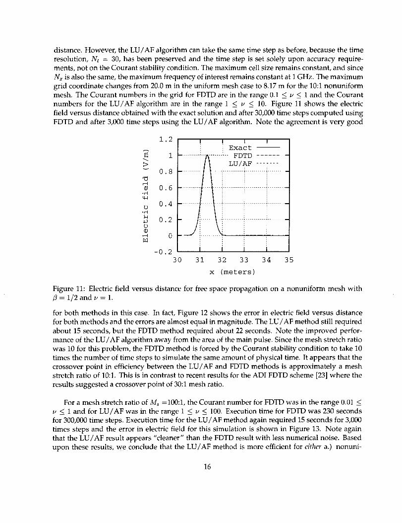
distance. However, the LU/AF algorithm can take the same time step as before, because the time

resolution, Nt = 30, has been preserved and the time step is set solely upon accuracy require-

ments, not on the Courant stability condition. The maximum cell size remains constant, and since

Nx is also the same, the maximum frequency of interest remains constant at 1 GHz. The maximum

grid coordinate changes from 20.0 m in the uniform mesh case to 8.17 m for the 10:1 nonuniform

mesh. The Courant numbers in the grid for FDTD are in the range 0.1 < L, < 1 and the Courant

numbers for the LU/AF algorithm are in the range 1 _< v < 10. Figure 11 shows the electric

field versus distance obtained with the exact solution and after 30,000 time steps computed using

FDTD and after 3,000 time steps using the LU/AF algorithm. Note the agreement is very good

1.2

0.8"0

0.6

q4

0.4O-4

0.2O

0

-0.2

I I I

Exact

i i......I I I I

30 31 32 33 34 35

x (meters)

Figure 11: Electric field versus distance for free space propagation on a nonuniform mesh with

fl = 1/2 and v = 1.

for both methods in this case. In fact, Figure 12 shows the error in electric field versus distance

for both methods and the errors are almost equal in magnitude. The LU/AF method still required

about 15 seconds, but the FDTD method required about 22 seconds. Note the improved perfor-

mance of the LU/AF algorithm away from the area of the main pulse. Since the mesh stretch ratio

was 10 for this problem, the FDTD method is forced by the Courant stability condition to take 10

times the number of time steps to simulate the same amount of physical time. It appears that the

crossover point in efficiency between the LU/AF and FDTD methods is approximately a meshstretch ratio of 10:1. This is in contrast to recent results for the ADI FDTD scheme [23] where the

results suggested a crossover point of 30:1 mesh ratio.

For a mesh stretch ratio of M_ =100:1, the Courant number for FDTD was in the range 0.01 <

v < ] and for LU/AF was in the range 1 < v _< 100. Execution time for FDTD was 230 seconds

for 300,000 time steps. Execution time for the LU/AF method again required 15 seconds for 3,000

times steps and the error in electric field for this simulation is shown in Figure 13. Note again

that the LU/AF result appears "cleaner" than the FDTD result with less numerical noise. Based

upon these results, we conclude that the LU/AF method is more efficient for either a.) nonuni-

16

>v

(1)-,-Iu_

D-_1

4JD(P

-,-I

0

4P

0 025

0.02

0 015

0.01

0 005

0

-0 005

-0.01

-0 015

-0.02

-0 025

30

! ! J i I........ _ ........ _. FDTD " -I

........i,i ......::._/..AF........:-.......t

f' IIi..it, - _ : : i_j

.... , -;_.......... !......... _:........

: t..J...!.......... i .......... i........ -I_i'!['"I ]i/'_'._"''''I f : : :

j ! : : :

L i' L_..i..-::.... i i j....... " " ""-: .......... :..........:........ 7

|l : : : J....... _.... [ J...._ ......... :.......... :........

: 1 1 ', : :

J I I I

31 32 33 34 35

x (meters)

Figure 12: Error in electric field versus distance for free space propagation on a nonuniform mesh

with a mesh stretch ratio of 10:1 and fl = 1/2, v = 1 (for FDTD).

>_.K]

-_1u_

O-,-I

_JD(1)

r-q

-,--I

O

0.03

0.02

0.01

0

-0.01

-0.02

-0.03

-0.043O

] I

........ l-i-t !

.......!:._.l.[.i

I:

I I I

i FDTD

::LU/AF

I

..... | --_ .......... ,....................

I

......... I--'! ...................... : ........

........ ..".... J..... :........... i........... ,........i

i i t I31 32 33 34 35

x (meters)

Figure 13: Error in electric field versus distance for free space propagation on a nonuniform mesh

with a mesh stretch ratio of 100:1 and fl = 1/2, _, = 1 (for FDTD).

17

form mesheswith largemeshstretchratiosor b.) a uniform mesh with a low frequency incident

excitation, where the pulse is highly resolved spatially over its entire frequency spectrum. Further

computational experience on additional free space propagation problems on nonuniform grids re-

veals that this sweeping method fails for large At (i.e. large Courant number). This can occur for

two reasons, even though the Fourier stability analysis indicates unconditional stability. First, it is

inapropriate to use a time step larger than one which propagates a wave over a distance compara-

ble to the entire solution domain in a single time step, and this can cause instability. Secondly, the

spatial sweeping process associated with each factor of the algorithm can itself become unstable

if it loses diagonal dominance, as observed by Jameson and Turkel [25]. Although a first-order

spatial upwind scheme guarantees diagonal dominance, there is a loss of diagonal dominance for

higher-order upwind schemes as the time step becomes asymptotically large. The upwind scheme

significantly increases the diagonal term compared with a centered scheme, however, and in ap-

plying the LU/AF scheme, this problem can be avoided by exercising care in selecting the time

step.

5.2 Lossy Dielectric Materials

To illustrate propagation in dielectric materials, the problem space was filled with a lossy di-

electric material with parameters _ -- 4_0, # = #0 and cr = 0.02. The pulse was allowed to prop-

agate on a uniform mesh for approximately 35 wavelengths at the minimum wavelength. Figure

14 shows the results of FDTD versus LU/AF with excellent agreement between the two methods.

A similar level of agreement is found with the same problem on a nonuniform grid.

0.015

0 Olbv

0.005

0

D"_ -0.005

D-0.01

-0.015

ZZZI/ CI Z......

...........-

I0 15 20 25 30 35

x (meters)

Figure 14: Electric field versus distance for propagation in a lossy dielectric on a uniform mesh

with fl = 1/9. and L, = 1.

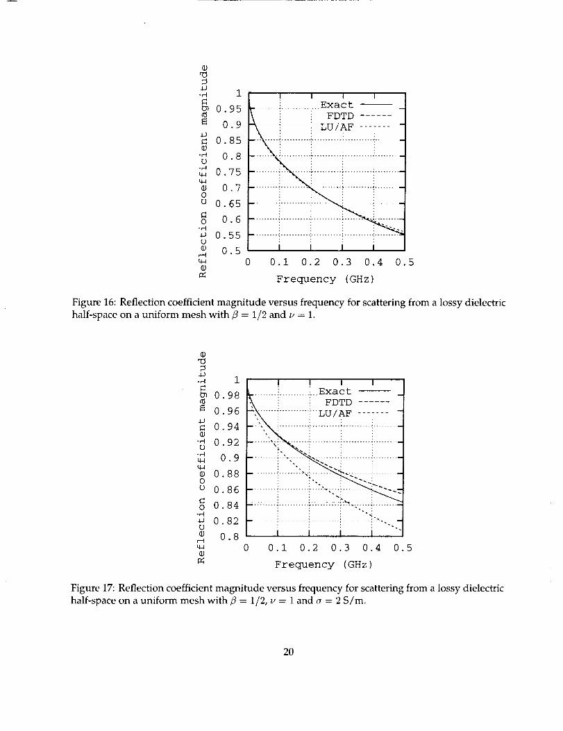
To illustrate the use of the LU/AF scheme for scattering problems, reflection from a lossy

dielectric half-space was considered as the benchmark problem. The dielectric interface scheme

18

of Section4.2 was implemented and the results are again compared with the FDTD method. To

solve this problem, the problem space is 2000 cells and it is filled with a lossy dielectric materialfrom cell numbers 751-2000. The total electric field is recorded versus time at cell number 750. The

incident field is obtained by running the code with free space only and recording the field versus

time at the same location. The incident field is subtracted from the total field to give the scattered

field. A point source located at the left boundary of the grid was used as the excitation source

and the dielectric half-space material parameters are E - 4_0,/_ -- I_0 and _ = 0.2 S/re. Figure

15 shows the time-domain scattered field for this case, and the agreement is excellent. Figure 16

0.35

"_ 0.3

m 0.25

0.2

0.15

-r_0.1

o 0.05-rq

0

o -0 05

m -0.i

-0.15

mTmm

B

....... }

....... ................

• i

0 i0 20 30 40 50 60

?DTD

I/AF

........ J........ :.......

Time (ns)

Figure 15: Scattered electric field versus time for scattering from a lossy dielectric half-space on a

uniform mesh with fl = 1/9. and _, -= 1.

shows the reflection coefficient results and again the agreement is excellent. The same problem

was run on the uniform mesh with cr = 2, and on a nonuniform mesh with a mesh stretch ratio of

10:1 and ¢ = 0.2 S/m. Figures 17 and 18 show the respective results.

Note that the LU/AF method produces more inaccurate results for moderate conductivity val-ues. This is due to the factorization error terms. As c_ is increased, the factorization errors become

larger. In principle, this factorization error can be reduced throught iterative error reduction [31].

This has been demonstrated for CFD problems [27], but it is not explored in the present work.

For perfect conductors, we simply set q = 0. Figure 18 shows that the LU/AF method is superior

on nonuniform grids, even for problems involving lossy dielectrics. These results indicate that

the physical dielectric boundary conditions have been properly implemented, thus making the

LU/AF method applicable to a wider class of problems.

6 Conclusions

This report has introduced a LU/AF implicit finite-difference method for computational elec-

tromagnetics. A second-order accurate, LU/AF, characteristic based algorithm for electromag-

19

(1)_3

__]-_ 1

0.95

0.9

O.85_)"_ 0.8O-4%4 0.75%4

0.7ou 0.65

o 0.6-M

0.55O

0 5r-_u_

I I I I.........................Exact J: FDTD

:_ ...................................................

I I I I

0 0.i 0.2 0.3 0.4 0.5

Frequency (GHz)

Figure 16: Reflection coefficient magnitude versus frequency for scattering from a lossy dielectric

half-space on a uniform mesh with fl = 1/2 and v = 1.

q)

.LJ•4 1

0.98

0.96

_J0.94

"_ 0.92o

%4 0.9%4

0.88oo 0.86

o 0.84

0.82O

0 8r-_%4

I I I I

,_, ........ i ........... !...Exact

i i FDTD

__! ....:: LU/AF ....... --'<i......................i..........i................... i?: ...... _4,_ ........ _.......... _:..........

........ - ....... ",..: ....... _'___ ,. ........ :..........

0 0.! 0.2 0.3 0.4 0.5

Frequency (GHz)

Figure 17: Reflection coefficient magnitude versus frequency for scattering from a lossy dielectric

half-space on a uniform mesh with fl = 1/2, _, = 1 and _ = 2 S/m.

20

0)_o

.,q

_ 0 9I_ "

_ 0 8(1) •

-r-tU

",-t_ 0.7

19000.6

o-_ 0.5.iJD©

q4

P_

I I I

_qL, i Exact........ [ ................. FDTD

i :: LU/AF .......

I dl I| , : ; "..... _l_:_ l-fr-,1--4 .................................

,li_k_li11!l._a t"i1: li_._l I ,4 , I:_ _. #, _I _ ,

__]'II II I:I I I 'I:' iI I _'I fl •I f-

___I' -I- -J-- -Il-.l|l'I.....!II #IJ-'_i'_ ] I,TT"--

: tJ.'t_!',]_L.t; rtf,Ii;' ii: ,:il_ '.!i:r'r_, t J,,j, .l

_; _'_', : _ ',l i! ',; iJ':; !J_

l I 'I I, , :_ ,, i, .I II I

.......... :............ :............ :..;_...;;., ;_.,..!!.,.L_, _ , I I iii ', II I I ii

I I' ' '

0 0.i 0.2 0.3 0.4 0.5

Frequency (GHz)

Figure 18: Reflection coefficient magnitude versus frequency for scattering from a lossy dielectric

half-space on a uniform mesh with fl = 1/2, _, = 1 and a = 0.2 S/m.

netics has been implemented and tested on one-dimensional model problems for uniform and

nonuniform grids. The one-dimensional model problem results for the characteristic based im-

plicit scheme demonstrate that:

.

.

Accurate solutions for wave propagation can be obtained using Courant number signifi-

cantly greater than one on nonuniform grids.

Stability of the implicit scheme allows a given amount of time to be covered in fewer time

steps than a conditionally stable scheme, and this can significantly improve efficiency when

nonuniform grids are needed. This is also extremely beneficial for low frequency excitation

sources where geometric details may force a highly oversampled mesh (uniform or nonuni-

form) in certain regions.

3. The method works well with lossy dielectric materials and perfect conductors.

4. The factorization error increases as cr increases, but it can be reduced in principle throughiterative error reduction.

5. The lowest dispersion and damping errors occur when fl = 1/2.

The present results demonstrate potential advantages in a one dimensional context, and this

approach appears promising for development of stable, accurate and efficient implicit LU/AF

schemes for complex two and three dimensional applications. Extensions to two and three-dimensional

applications have been outlined [31], but details of this work will the subject of future reports andarticles.

21

References

[11 K. S. Yee, "Numerical solution of initial boundary value problems involving Maxwell's equa-

tions in isotropic media," IEEE Transactions on Antennas and Propagation, vol. 14, no. 3, pp.

302-307, Mar. 1966.

[2] K. S. Kunz and R. J. Luebbers, The Finite Difference Time Domain Method for Electromagnetics,

CRC Press, Boca Raton, FL, 1993.

[3] A. Taflove, Computational Electrodynamics: The Finite-Difference Time-Domain Method, Artech

House, Boston, MA, 1995.

[4] A. Taflove, Ed., Advances in Computational Electrodynamics: The Finite-Difference Time-Domain

Method, Artech House, Boston, MA, 1998.

[5]

[6]

[71

[81

[91

[lO1

[11]

R. Holland, L. Simpson, and K. Kunz, "Finite-difference analysis of EMP coupling to lossy

dielectric structures," IEEE Transactions on Electromagnetic Compatibility, vol. EMC-22, no. 3,

pp. 203-20% Aug. 1980.

R. F. Warming and R. M. Beam, "An extension of a-stability to alternating direction implicit

methods," B/T, vol. 19, pp. 395-417, 1979.

R. C. Buggetn W. R. Briley and H. McDonald, "Solution of the three-dimensional navier

stokes equations for a steady laminar horseshoe vortex fow," in Proc. 7th Computational Fluid

Dynamics Conference, Cincinnati, OH, July 1985, AIAA Paper 85-1520-CP.

W. F. Hall V. Shankar and A. H. Mohammadian, "A time-domain differential solver for elec-

tromagnetic problems," Proc. IEEE, vol. 77, no. 5, pp. 709-721, May 1989.

W. F. Hall V. Shankar and A. H. Mohammadian, "A time-domain, finite-volume treatment

for the Maxwell equations," Electromagnetics, vol. 10, pp. 127, 1990.

J. S. Shang, "Characteristic based methods for the time-domain Maxwell equations," in AIAA

29th Aerospace Sciences Meeting & Exhibit, Reno, NV, Jan. 1991, vol. AIAA 91-0606.

J. S. Shang, "A characteristic-based algorithm for solving 3-d time-domain Maxwell equa-

tions," in AIAA 30th Aerospace Sciences Meeting & Exhibit, Reno, NV, Jan. 1992, vol. AIAA92-0452.

[12] J. S. Shang, "A fractional-step method for solving 3-d time-domain Maxwell equations," in

AIAA 31st Aerospace Sciences Meeting & Exhibit, Reno, NV, Jan. 1993, vol. AIAA 93-0461.

[13]

[14]

J. S. Shang and D. Gaitonde, "Characteristic-based, time-dependent Maxwell equations

solvers on a general curvilinear frame," in AIAA 24th Plasmadynamics & Lasers Conference,

Orlando, FL, July 1993, vol. AIAA 93-3178.

K. C. Hill J. S. Shang and D. Calahan, "Performance of a characteristic-based, 3-d time-

domain Maxwell equations solvers on a massively parallel computer," in AIAA 24th Plasma-

dynamics & Lasers Conference, Orlando, FL, July 1993, vol. AIAA 93-3179.

22

[15]

[16]

[17]

[18]

[19]

[20]

[21]

[22]

[23]

[24]

[25]

[26]

[27]

[28]

J. S. Shang and R. M. Fithen, "A comparative study of numerical algorithms for computa-

tional electromagnetics," in AIAA 25th Plasmadynamics & Lasers Conference, Colorado Springs,

CO, June 1994, voI. AIAA 94-2410.

J. S. Shang and D. Gaitonde, "Characteristic-based, time-dependent Maxwell equation

solvers on a general curvilinear frame," AIAA Journal, vol. 33, no. 3, pp. 491-498, March1995.

J. S. Shang, "A fractional-step method for solving 3d, time-domain Maxwell equations/'

Journal of Comp. Phys., vol. 118, pp. 109-119, 1995.

J. S. Shang and R. M. Fithen, "A comparative study of characteristic-based algorithms for the

Maxwell equations," Journal of Comp. Phys., vol. 125, pp. 378-394, 1996.

D. C. Blake and J. S. Shang, "A procedure for rapid prediction of electromagnetic scattering

from complex objects," in AIAA 29th Plasmadynamics & Lasers Conference, Albuquerque, NM,

June 1998, vol. AIAA 98-2925.

D. Gaitonde and J. S. Shang, "High-order finite-volume schemes in wave propagation phe-

nomena," in AIAA 27th Plasmadynamics & Lasers Conference, New Orleans, LA, June 1996, vol.AIAA 96-2335.

F. Zheng, Z. Chen, and J. Zhang, "A finite-difference time-domain method without the

Courant stability conditions," IEEE Microwave Guided Wave Letters, vol. 9, no. 11, pp. 441-443, Nov. 1999.

F. Zheng, Z. Chen, and J. Zhang, "Toward the development of a three-dimensional uncondi-

tionally stable finite-difference time-domain method," IEEE Transactions on Microwave Theory

and Techniques, vol. 48, no. 9, pp. 1550-1558, Sept. 2000.

T. Namiki, "3-D ADI-FDTD method--Unconditionally stable time-domain algorithm for

solving full vector Maxwell's equations," IEEE Transactions on Microwave Theory and Tech-

niques, vol. 48, no. 10, pp. 1743-1748, Oct. 2000.

A. Taflove and S. Hagness, Computational Electrodynamics: The Finite-Difference Time-Domain

Method, 2 ed., Artech House, Boston, MA, 2000.

A. Jameson and E. Turkel, "Implicit schemes and approximate factorizations," Math. Comp.,

vol. 37, pp. 385-397, 1981.

D. M. Belk and D. L. Whitfield, "Unsteady three-dimesional euler solutions on blocked grids

using an implicit two-pass algorithm," January 1987, vol. AIAA Paper No. 87-0450.

W. R. Briley, S. S. Neerarambam, and D. L. Whitfield, "Implicit Lower-Upper/Approximate-

Factorization algorithms for incompressible fows," Journal of Comp. Phys., vol. 128, pp. 32-42,1996.

J. L. Steger and R. E Warming, "Flux vector splitting of the invisid gas dynamic equations

with applications to finite difference methods," Journal of Comp. Phys., vol. 4, no. 2, pp. 263-293, 1981.

23

[29] Z. P.Liao, H. L. Wong,B.-P.Yang,and Y.-F.Yuan, "A transmitting boundary for transientwaveanalysis,"Sci. Sin., Ser. A, vol. 27, no. 10, pp. 1063-1076, Oct. 1984.

[30] J.-P. Berenger, "A perfectly matched layer for the absorption of electromagnetic waves,"

Journal of Computational Physics, vol. 114, no. 1, pp. 185--200, 1994.

[31] J. H. Beggs and W. R. Briley, "An implicit characteristic based method for computational

electromagnetics," Tech. Rep. MSSU-EIRS-ERC-98-11, Miss. State Univ., August 1998.

24

REPORT DOCUMENTATION PAGE FormApprovedOMB No. 0704-0188

Public repo_ng burden for tbls collection of information is estimated to average 1 hour per response, including the time for reviewing instructions, searching extsting data sources,

gathering and maintaining the data needed, and completing and reviewing the coflestion of information. Send comments regarding this burden estimate or any other aspect of this

coIlecSon of _nf0rmation, incJuding suggestions for reducing this burden, to Washington Headquarters Services, Directorate for Information Operations and Reports, 1215 Jefferson Davis

Highway, Suite 1204, Adthgton, VA 22202-4302, and to the Office of Management and Budget, Paperwork Reduction Project 0704-0188}, Washington, DC 20503.

1. AGENCY USE ONLY (Leave blank) 2. REPORT DATE 3. REPORT TYPE AND DATES COVERED

May 2001 Technical Memorandum

4. TITLE AND SUBTrh.E 5. FUNDING NUMBERS

An Implicit Characteristic Based Method for Electromagnetics 706-31-41-01

6. AUTHOR(S)

John H. Beggs, W. Roger Briley

7. PERFORMINGORGANIZATIONNAME(S)ANDADDRESS(ES)NASA Langley Research Center

Hampton, VA 23681-2199

9. SPONSORING/MONITORING AGENCY NAME(S) AND ADDRESS(ES)

National Aeronautics and Space Administration

Washington, DC 20546-0001

11.SUPPLEMENTARY NOTES

8. PERFORMING ORGANIZATIONREPORT NUMBER

L-18051

10. SPONSORING/MONITORINGAGENCY REPORT NUMBER

NASA/TM-2001-210862

12a. DISTRIBUTION/AVAILABILITY STATEMENT

Unclassified-Unlimited

Subject Category 33 Distribution: StandardAvailability: NASA CASI (301) 621-0390

12b. DISTRIBUTION CODE

13. ABSTRACT (Maximum 200 words)

An implicit characteristic-based approach for numerical solution of Maxwelrs time-dependent curl equations in fluxconservative form is introduced. This method combines a characteristic based finite difference spatialapproximation with an implicit lower-upper approximate factorization (LU/AF) time integration scheme. Thisapproach is advantageous for three-dimensional applications because the characteristic differencing enables atwo-factor approximate factorization that retains its unconditional stability in three space dimensions, and it doesnot require solution of tridiagonal systems. Results are given both for a Fourier analysis of stability, damping anddispersion properties, and for one-dimensional model problems involving propagation and scattering for free spaceand dielectric materials using both uniform and nonuniform grids. The explicit FDTD algorithm is used as aconvenient reference algorithm for comparison. The one-dimensional results indicate that for low frequency

problems on a highly resolved uniform or nonuniform grid, this LU/AF algorithm can produce accurate solutions atCourant numbers significantly greater than one, with a corresponding improvement in efficiency for simulating agiven period of time. This approach appears promising for development of dispersion optimized LU/AF schemesfor three dimensional applications.

14. SUBJECT TERMS

computational electromagnetics, FDTD methods

17. SECURITY CLASSIFICATION

OF REPORT

Unclassified

18. SECURITY CLASSIFICATIONOF THIS PAGE

Unclassified

NSN 7540-01-280-5500

19. SECURITY CLASSIFICATIONOF ABSTRACT

Unclassified

15. NUMBER OF PAGES

29

16. PRICE CODE

A03

20. LIMITATION OF ABSTRACT

Standard Form 298 (Rev. 2-89)Prescribed by ANSI Std. Z39-18298-102