an external memory data structure for shortest path queries
TRANSCRIPT

Discrete Applied Mathematics 126 (2003) 55–82
An external memory data structure for shortestpath queries�
David Hutchinsona , Anil Maheshwarib;1 , Norbert Zehb;∗aDepartment of Computer Science, Duke University, Durham, NC, USA
bSchool of Computer Science, Carleton University, 1125 Colonel By Drive, Ottawa, Ont.,Canada K1S 5B6
Received 22 September 1999; received in revised form 28 November 2000; accepted 7 September 2001
Abstract
We present results related to satisfying shortest path queries on a planar graph stored inexternal memory. Let N denote the number of vertices in the graph and sort(N ) denote thenumber of input=output (I=O) operations required to sort an array of length N :
(1) We describe a blocking for rooted trees to support bottom-up traversals of these trees inO(K=B) I=Os, where K is the length of the traversed path. The space required to store thetree is O(N=B) blocks, where N is the number of vertices of the tree and B is the blocksize.
(2) We give an algorithm for computing a 23 -separator of size O(
√N ) for a given embedded
planar graph. Our algorithm takes O(sort(N )) I=Os, provided that a breadth-8rst spanningtree is given.
(3) We give an algorithm for triangulating embedded planar graphs in O(sort(N )) I=Os.
We use these results to construct a data structure for answering shortest path queries on planargraphs. The data structure uses O(N 3=2=B) blocks of external memory and allows for a shortestpath query to be answered in O((
√N +K)=DB) I=Os, where K is the number of vertices on the
reported path and D is the number of parallel disks. ? 2002 Elsevier Science B.V. All rightsreserved.
Keywords: External-memory algorithms; Graph algorithms; Shortest paths; Planar graphs
� A preliminary version appeared in [14].∗ Corresponding author.E-mail addresses: [email protected] (D. Hutchinson), [email protected] (A. Maheshwari),
[email protected] (N. Zeh).1 Research supported by NSERC and NCE GEOIDE.
0166-218X/02/$ - see front matter ? 2002 Elsevier Science B.V. All rights reserved.PII: S0166 -218X(02)00217 -2
56 D. Hutchinson et al. / Discrete Applied Mathematics 126 (2003) 55–82
1. Introduction
Answering shortest path queries in graphs is an important and intensively stud-ied problem. It has applications in communication systems, transportation problems,scheduling, computation of network Gows, and geographic information systems (GIS).Typically, an underlying geometric structure is represented by a combinatorial structure,which is often a weighted planar graph.The motivation to study external memory shortest path problems arose in our GIS
research and in particular, with an implementation of the results in [16] for shortest pathproblems in triangular irregular networks. In this application the given graph representsa planar map, i.e., it is planar and embedded. Quite commonly it is too large to 8t intothe internal memory of even a large supercomputer. In this case, and in many otherlarge applications, the computation is forced to wait while large quantities of dataare transferred between relatively slow external (disk-based) memory and fast internalmemory. Thus, the classical internal memory approaches to answering shortest pathqueries in a planar graph (e.g. [6,8–10,15]) may not work eIciently when the datasets are too large.
1.1. Model of computation
Unfortunately, the I=O-bottleneck is becoming more signi8cant as parallel computinggains popularity and CPU speeds increase, since disk speeds are not keeping pace [22].Thus, it is important to take the number of input=output (I=O) operations performed byan algorithm into consideration when estimating its eIciency. This issue is capturedin the parallel disk model (PDM) [24], as well as a number of other external memorymodels [5,25]. We adopt the PDM as our model of computation for this paper due toits simplicity, and the fact that we consider only a single processor.In the PDM, an external memory, consisting of D disks, is attached to a machine
with an internal memory capable of holding M data items. Each of the disks is dividedinto blocks of B consecutive data items. Up to D blocks, at most one per disk, canbe transferred between internal and external memory in a single I=O operation. Thecomplexity of an algorithm is the number of I=O operations it performs.
1.2. Previous results
Shortest path problems can be divided into three general categories: (1) computinga shortest path between two given vertices of a graph, (2) computing shortest pathsbetween a given source vertex and all other vertices of a graph (single source shortestpaths (SSSP) problem), and (3) computing the shortest paths between all pairs ofvertices in a graph (all pairs shortest paths (APSP) problem).
Previous results in the RAM model: In the sequential RAM model, much workhas been done on shortest path problems. Dijkstra’s algorithm [6], when implementedusing Fibonacci heaps [11], is the best-known algorithm for the SSSP-problem forgeneral graphs (with nonnegative edge weights). It runs in O(|E| + |V | log |V |) time,where |E| and |V | are the numbers of edges and vertices in the graph, respectively.
D. Hutchinson et al. / Discrete Applied Mathematics 126 (2003) 55–82 57
The APSP-problem can be solved by applying Dijkstra’s algorithm to all verticesof the graph, which results in an O(|V‖E| + |V |2 log |V |) running time. For planargraphs, an O(N
√logN )-algorithm for the SSSP-problem and an O(N 2)-algorithm for
the APSP-problem, where N = |V |, are given in [9]. A linear-time SSSP-algorithm forplanar graphs is presented in [15].An alternate approach is to preprocess the given graph for online shortest path
queries. For graphs for which an O(√
N )-separator theorem holds (e.g., planar graphs),an O(S)-space data structure (N 6 S6N 2) that answers distance queries in O(N 2=S)time is presented in [8]. The corresponding shortest path can be reported in time pro-portional to the length of the reported path. (For planar graphs slightly better boundsare given.)It is known that every tree or outerplanar graph has a 2
3 -separator of size O(1).In [17] it is shown that every planar graph has a 2
3 -separator of size O(√
N ), and alinear-time algorithm for 8nding such a separator is given. Other results include separa-tor algorithms for graphs of bounded genus [1] and for computing edge-separators [7].
Previous results in the PRAM model: A PRAM algorithm for computing a 23 -
separator of size O(√
N ) for a planar graph is presented in [12]. The algorithm runsin O(log2 N ) time and uses O(N 1+�) processors, where � ¿ 0 is a constant. In [13]a PRAM algorithm is given that computes a planar separator in O(logN ) time usingO(N=logN ) processors, provided that a breadth-8rst spanning tree (BFS-tree) of thegraph is given.
Previous results in external memory: In the PDM, sorting, permuting, and scanningan array of size N take sort(N ) = O((N=DB) logM=BN=B); perm(N ) = O(min{N; sort(N )}), and scan(N )=O(N=DB) I=Os [23,24]. For a comprehensive survey on externalmemory algorithms, refer to [23]. The only external-memory shortest path algorithmknown to us is the SSSP-algorithm in [4], which takes O(|V |=D+(|E|=DB) logM=B|E|=B)I=Os with high probability, on a random graph with random weights. We do not knowof previous work on computing separators in external memory; but one can use thePRAM-simulation results in [3] together with the results of [12,13] cited above. Un-fortunately, the PRAM simulation introduces O(sort(N )) I=Os for every PRAM step,and so the resulting I=O complexity is not attractive for this problem.
1.3. Our results
The main results of this paper are:
(1) A blocking to store a rooted tree T in external memory so that a path of lengthK towards the root can be traversed in at most �K=�DB�+3 I=Os, for 0¡ � ¡ 1.If �¿ 3−√
52 , the blocking uses at most (2+2=(1−�))|T |=B+D blocks of external
storage. For � ¡ 3−√5
2 , a slight modi8cation of the approach reduces the amountof storage to (1 + 1=(1 − 2�))|T |=B + D blocks. For 8xed �, the tree occupiesoptimal O(|T |=B) blocks of external storage and traversing a path takes optimalO(K=DB) I=Os. Using the best previous result [20], the tree would use the same

58 D. Hutchinson et al. / Discrete Applied Mathematics 126 (2003) 55–82
amount of space within a constant factor, but traversing a path of length K wouldtake O(K=logd(DB)) I=Os, where d is the maximal degree of the vertices in thetree (see Section 3).
(2) An external memory algorithm which computes a separator consisting of O(√
N )vertices for an embedded planar graph in O(sort(N )) I=Os, provided that a BFS-tree of the graph is given. Our algorithm is based on the classical planar separatoralgorithm in [17]. The main challenge in designing an external memory algorithmfor this problem is to determine a good separator corresponding to a fundamentalcycle (see Section 4).
(3) An external memory algorithm which triangulates an embedded planar graph inO(sort(N )) I=Os (see Section 5).
(4) An external memory data structure for answering shortest path queries online. Re-sults 1–3, above, are the main techniques that we use to construct this data struc-ture. Our data structure uses O(N 3=2=B) blocks of external memory and answersonline distance and shortest path queries in O(
√N=DB) and O((
√N + K)=DB)
I=Os, respectively, where K is the number of vertices on the reported path (seeSection 6).
Our separator and triangulation algorithms may be of independent interest, since graphseparators are used in the design of eIcient divide-and-conquer graph algorithms andmany graph algorithms assume triangulated input graphs.
2. Preliminaries
2.1. De3nitions
An undirected graph (or graph for short) G = (V; E) is a pair of sets V and E,where V is called the vertex set and E is called the edge set of G. Each edge in Eis an unordered pair {v; w} of vertices v and w in V . Unless stated otherwise, we use|G| to denote the cardinality of V . In a directed graph, every edge is an ordered pair(v; w). In this case, we call v the source vertex and w the target vertex of edge (v; w).A graph G is planar if it can be drawn in the plane so that no two edges intersect,except possibly at their endpoints. Such a drawing de8nes for each vertex v of G, anorder of the edges incident to v clockwise around v. We call G embedded if we aregiven this order for every vertex of G. By Euler’s formula, |E|6 3|V | − 6 for planargraphs.A path from a vertex v to a vertex w in G is a list p = 〈v = v0; v1; : : : ; vk = w〉
of vertices, where {vi; vi+1}∈E for 06 i ¡ k. The length of path p is the numberk of edges in the path. We call p a cycle if v0 = vk . Paths and cycles are de8nedanalogously for directed graphs. A directed acyclic graph (DAG) is a directed graphthat does not contain cycles of length ¿ 0. A graph G is connected if there is a pathbetween any two vertices in G. A subgraph G′=(V ′; E′) of G is a graph with V ′ ⊆ Vand E′ ⊆ E. Given a subset X ⊆ V , we denote by G[X ] = (X; E[X ]) the subgraph ofG induced by X , where E[X ] = {{v; w}∈E: {v; w} ⊆ X }. The graph G–X is de8ned

D. Hutchinson et al. / Discrete Applied Mathematics 126 (2003) 55–82 59
as G[V \X ]. The connected components of G are the maximal connected subgraphs ofG. A tree with N vertices is a connected graph with N − 1 edges. A rooted tree is atree with a distinguished root vertex. The level or depth of a vertex v in a rooted treeis the number of edges on the path from v to the root. For an edge {v; w} in a tree Twe say that v is w’s parent and w is v’s child if w’s depth in T is greater than v’s. Avertex v is an ancestor of a vertex w, and w is a descendant of v, if v is w’s parentor it is an ancestor of w’s parent. A common ancestor of two vertices v and w is avertex u which is an ancestor of v and w. The lowest common ancestor (lca)(v; w) ofv and w is the common ancestor of v and w at maximum depth among all commonancestors of v and w. A preorder numbering of a rooted tree T with N vertices is anassignment of numbers 0 through N − 1 to the vertices of T such that every vertexhas a preorder number less than any of its descendants and the preorder numbers ofeach vertex and all its descendants are contiguous. Given an ordering of the childrenof each node, a lexicographical numbering of T is a preorder numbering of T suchthat the preorder numbers of the children of any node, sorted by the given order, areincreasing. An independent set I ⊆ V in a graph G is a set of vertices such that forevery vertex v∈ I and every edge {v; w}∈E, w �∈ I . That is, no two vertices in I areadjacent. A k-coloring of a graph G is an assignment f :V → {1; : : : ; k} of colors tothe vertices of G such that for any edge {v; w}∈E, f(v) �=f(w).
A spanning tree of a graph G=(V; E) is a tree T =(V; F), where F ⊆ E. A BFS-treeis a rooted spanning tree T of G such that for any edge {v; w} in G, the levels of vand w in T diPer by at most 1.Let c :E → R+ be an assignment of non-negative costs to the edges of G. The cost
‖p‖ of a path p = 〈v0; : : : ; vk〉 is de8ned as ‖p‖=∑k−1i=0 c({vi; vi+1}). A shortest path
&(v; w) is a path of minimal cost from v to w.Let w :V → R+ be an assignment of non-negative weights to the vertices of G
such that∑
v∈V w(v)6 1. The weight w(H) of a subgraph H of G is the sum of theweights of the vertices in H . An �-separator, 0¡ � ¡ 1, of G is a subset S of V suchthat none of the connected components of G − S has weight exceeding �.For a given DAG G = (V; E), a topological ordering is a total order O ⊆ V × V
such that for every edge (v; w)∈E, (v; w)∈O.We will describe results on paths in a rooted tree which originate at an arbitrary
node of the tree and proceed to the root. We will refer to such paths as bottom-uppaths.For a given block size B, a blocking of a graph G = (V; E) is a decomposition of
V into vertex sets B1; : : : ;Bq such that V =⋃q
i=1 Bi and |Bi|6B. The vertex sets Bi
do not have to be disjoint. Each such vertex set Bi corresponds to a block in externalmemory where its vertices are stored.
2.2. External memory techniques
First, we introduce some useful algorithmic techniques in external memory whichwe will use in our algorithms. These include external memory stacks and queues, listranking, time-forward processing and their applications to processing trees.

60 D. Hutchinson et al. / Discrete Applied Mathematics 126 (2003) 55–82
We have already observed that scanning an array of size N takes O(scan(N )) I=Osusing at least D blocks of internal memory to hold the D blocks currently beingscanned. Using 2D blocks of internal memory, a series of N stack operations can beexecuted in O(scan(N )) I=Os. These 2D blocks hold the top-most elements on thestack. Initially, we hold the whole stack in internal memory. As soon as there are 2DBelements on the stack, and we want to push another element on the stack, we swapthe DB bottom-most elements to external memory. This takes one I=O. Now it takesat least DB stack operations (DB pushes to 8ll the internal buPer again or DB popsto have no elements left in internal memory) before the next I=O becomes necessary.Thus, we perform at most one I=O per DB stack operations, and N stack operationstake O(N=DB)=O(scan(N )) I=Os. Similarly, to implement a queue, we need 2D blocksof internal memory, D to buPer the inputs at the end of the queue and D to buPer theoutputs at the head of the queue.The list-ranking problem is the following: Given a singly linked list L and a pointer
to its head, compute for every node of L its distance to the tail of L. A commonvariant is to assign weights to the nodes of L and to compute for every node theweight of the sublist of L starting at this node. In [3], a recursive list-ranking procedurewas developed. If the list has size at most M , the problem can be solved in internalmemory. Reading the input and writing the output take O(scan(N )) I=Os in this case.If the list contains more than M nodes the procedure 3-colors the list and removes thelargest monochromatic set of vertices. For every removed vertex x, the weight of x’spredecessor y is updated to w(y) = w(y) + w(x). After recursively applying the sametechnique to the remaining sublist, which has size at most 2
3N , the removed vertices arereintegrated into the list and their ranks computed. In [3] it is shown that the 3-coloringof the list and the removal and reintegration of the independent set can be done inO(sort(N )) I=Os. Thus, this procedure takes T (N )6T ( 23N )+O(sort(N ))=O(sort(N ))I=Os. In [26] it is shown that the 3-coloring technique can be extended to rooted trees,which allows the application of the same framework to the problem of computing thelevel of every node in a rooted tree. Alternatively, one can use the Euler-tour techniquetogether with the list-ranking technique to compute these levels.The Euler-tour technique can be described as follows: Given a rooted tree T , we
replace every edge {v; w} by two directed edges (v; w) and (w; v). For every vertex v,let e0; : : : ; ek−1 be the incoming edges of v and e′0; : : : ; e
′k−1 be the outgoing edges of
v, where e′i is directed opposite to ei. We de8ne edge e′(i+1) mod k to be the successorof edge ei, for 06 i ¡ k. At the root of T we de8ne edge e′k−1 to have no successor.This de8nes a traversal of the tree, starting at the root and traversing every edge of thetree exactly twice, once per direction. To compute the levels of all vertices in T , forinstance, we assign weight 1 to all edges directed from parents to children and weight−1 to all edges directed from children to parents. Then we can apply the list-rankingtechnique to compute the levels of the endpoints of all edges.If we choose the order of the edges e0; : : : ; ek−1 carefully, we can use the Euler-tour
technique to compute a lexicographical numbering of a given rooted tree. Recall thatin this case we are given a left to right ordering of the children of every vertex. Weconstruct the Euler tour by choosing for every vertex v edge e0 to be the edge connect-ing v to its parent. The remaining edges e1; : : : ; ek−1 are the edges connecting v to its

D. Hutchinson et al. / Discrete Applied Mathematics 126 (2003) 55–82 61
children, sorted from left to right. It is easy to see that the Euler tour thus constructedtraverses the tree T lexicographically. To compute the lexicographical numbers of allvertices, we assign weight 1 to edges directed from parents to children and weight 0 toall remaining edges. After applying list ranking to this list, the lexicographical numberof a vertex v is the rank of the edge with weight 1 and target vertex v.An important ingredient of the 3-coloring technique in [3] as well as most of the
algorithms presented in this paper is time-forward processing, which was introduced in[3]. This technique is useful for processing DAGs. We view the DAG as a circuit andallow sending a constant amount of information along every edge. Every node can usethe information sent along its incoming edges to compute a function of these valuesand then send a constant amount of information along each of its outgoing edges. Thetechnique presented for this problem in [3] has two constraints: (1) the fan-in of thevertices in the DAG has to be bounded by some constant d and (2) the ratio m=M=Bhas to be large enough. These constraints have been removed in [2] using the followingelegant solution: Given a DAG G, sort the vertex set topologically, which de8nes atotal order on this set. Then evaluate the nodes in their order of appearance, therebyensuring that all nodes u with an outgoing edge (u; v) have been evaluated beforev. Every such node u inserts the information it wants to send to v into a priorityqueue, giving it priority v. Node v performs din(v) DELETEMIN operations to retrieveits inputs, where din(v) is the fan-in of v. It is easy to verify that at the time whenv is evaluated, the din(v) smallest elements in the priority queue have indeed priorityv. After sorting the vertex and edge sets of the DAG, this technique performs 2|E|priority queue operations, which take O(sort(|E|)) I=Os [2]. Thus, this technique takesO(sort(|V |+ |E|)) I=Os.
3. Blocking rooted trees
In this section, we consider the following problem: Given a rooted tree T , store itin external memory so that for any query vertex v∈T , the path from v to the rootof T can be reported I=O-eIciently. One can use redundancy to reduce the numberof blocks that have to be read to report the path. However, this increases the spacerequirements. The following theorem gives a trade-oP between the space requirementsof the blocking and the I=O-eIciency of the tree traversal.
Theorem 1. Given a rooted tree T of size N and a constant �; 0¡ � ¡ 1; we can storeT on D parallel disks so that traversing any bottom-up path of length K in T takes atmost �K=�DB�+3 I=Os. The amount of storage used is at most (2+2=(1−�))N=B+Dblocks for �¿ 3−√
52 and at most (1 + 1=(1− 2�))N=B + D blocks for � ¡ 3−√
52 .
Proof. This follows from Lemmas 2 and 3 below.
Intuitively, our approach is as follows. We cut T into layers of height �DB. Thisdivides every bottom-up path of length K in T into subpaths of length �DB; eachsubpath stays in a particular layer. We ensure that each such subpath is stored in

62 D. Hutchinson et al. / Discrete Applied Mathematics 126 (2003) 55–82
Fig. 1. A tree is cut into layers of height �DB. (Here, �DB=2.) The tree is cut along the dashed lines. Theresulting subtrees Ti are shaded.
at most D blocks, and each of the D blocks is stored on a diPerent disk. Thus eachsubpath can be traversed at the cost of a single I=O operation. This gives us the desiredI=O-bound because any bottom-up path of length K crosses at most �K=�DB�+1 layersand is thus divided into at most �K=�DB�+ 1 subpaths.More precisely, let h represent the height of T , and let h′ = �DB be the height
of the layers to be created (we assume that h′ is an integer). We cut T into layersL0; : : : ; L�h=h′�−1, where layer Li is the subgraph of T induced by the vertices on levelsih′ through (i+1)h′−1 (see Fig. 1). Each layer is a forest of rooted trees, whose heightsare at most h′. Suppose that there are r such trees, T1; : : : ; Tr , taken over all layers.We decompose each tree Ti, 16 i6 r, into possibly overlapping subtrees Ti;0; : : : ; Ti; s
having the following properties:
Property 1. |Ti; j|6DB; for all 06 j6 s.
Property 2.∑s
j=0 |Ti; j|6 (1 + 1=(1− �))|Ti|.
Property 3. For every leaf l of Ti; there is a subtree Ti; j containing the whole pathfrom l to the root of Ti.
Lemma 2. Given a rooted tree Ti of height at most �DB; 0¡ � ¡ 1; we can decomposeTi into subtrees Ti;0; : : : ; Ti; s having Properties 1–3.
Proof. If |Ti|6DB; we “decompose” Ti into one subtree Ti;0 = Ti. Then Properties1–3 trivially hold. So assume that |Ti|¿ DB.Given a preorder numbering of the vertices of Ti, we denote every vertex by its
preorder number. Given a parameter 0¡ t ¡ DB to be speci8ed later, let s=�|Ti|=t�−1.We de8ne vertex sets V0; : : : ; Vs, where Vj={jt; : : : ; (j+1)t−1} for 06 j6 s (see Fig.2(a)). The vertex set Vs may contain less than t vertices. The tree Ti; j = Ti(Vj) is thesubtree of Ti consisting of all vertices in Vj and their ancestors in Ti (see Fig. 2(b)).We claim that these subtrees Ti; j have Properties 1–3, if we choose t appropriately.

D. Hutchinson et al. / Discrete Applied Mathematics 126 (2003) 55–82 63
Fig. 2. (a) A rooted tree Ti with its vertices labelled with their preorder numbers. Assuming that t=8, V0 isthe set of black vertices, V1 is the set of gray vertices, and V2 is the set of white vertices. (b) The subtreesTi(V0); Ti(V1), and Ti(V2) from left to right.
Property 3 is guaranteed because for every leaf l, the subtree Ti; j, where l∈Vj,contains the whole path from l to the root of Ti. To prove Property 1, let Aj be theset of vertices in Ti; j which are not in Vj. Every such vertex x is an ancestor ofsome vertex y¿ jt. That is, x ¡ y. As x �∈ Vj and the vertices in Vj are numberedcontiguously, x ¡ jt. Vertex y is in the subtree of Ti rooted at x and x ¡ jt6y. Thus,vertex jt must be in this subtree as well because the vertices in the subtree rooted at xare numbered contiguously. Hence, every vertex in Aj is an ancestor of vertex jt. Thisimplies that |Aj|6 �DB because jt has at most one ancestor at each of the at most�DB levels in Ti. Hence, |Ti; j| = |Aj| + |Vj|6 �DB + t. Choosing t = DB − �DB, weguarantee that every subtree Ti; j has size at most DB. Now Property 2 holds because
s∑j=0
|Ti; j|6�|Ti|=(DB−�DB)�−1∑
j=0
DB (1)
6( |Ti|
DB − �DB+ 1
)DB (2)
=1
1− �|Ti|+ DB (3)
¡(
11− �
+ 1)|Ti|: (4)
The step from lines (3) to (4) uses the fact that |Ti|¿ DB.
Lemma 3. If a rooted tree T of size N is decomposed into subtrees Ti; j such thatProperties 1–3 hold; T can be stored on D parallel disks so that any bottom-up pathof length K in T can be traversed in at most �K=�DB�+ 3 I=Os; for 0¡ � ¡ 1. For�¿ 3−√
52 ; the amount of storage used is at most (2 + 2=(1− �))N=B+D blocks. For
� ¡ 3−√5
2 ; the tree occupies at most (1 + 1=(1− 2�))N=B + D blocks.
Proof. We consider D disks of block size B as one large disk divided into superblocksof size DB. Thus; by Property 1; each subtree Ti; j 8ts into a single superblock and canbe read in a single I=O.

64 D. Hutchinson et al. / Discrete Applied Mathematics 126 (2003) 55–82
A bottom-up path p of length K in T crosses at most k = �K=�DB�+1 layers. Thisdivides p into k maximal subpaths such that none of them crosses more than one layer.Each such subpath p′ is a leaf-to-root path in some subtree Ti, or a subpath thereof.Thus, by Property 3, there exists a subtree Ti; j that contains the whole of the subpathp′. That is, each subpath p′ can be accessed in a single I=O. Therefore, the traversalof p takes at most �K=�DB�+ 1 I=Os.By Property 2, all subtrees Ti; j together use at most (1+ 1=(1− �))
∑ri=0 |Ti|= (1+
1=(1−�))N space. Initially, we store every subtree Ti; j in a separate superblock, whichmay leave many superblocks sparsely populated. As long as there are at least twosuperblocks that are at most half full we keep merging pairs of superblocks. Finally,if we are left with a single half full superblock we try to 8nd a superblock that can bemerged with it. If we 8nd one, we merge the two superblocks. Otherwise, the half-fullsuperblock together with any other superblock contains more than DB vertices. All othersuperblocks are at least half full. Thus, on average, each superblock is at least half full,and we use �(2− 2=(1− �))N=DB� superblocks, i.e., D�(2− 2=(1− �))N=DB�6 (2 +2=(1− �))N=B + D blocks to store all subtrees Ti; j.For � ¡ 3−√
52 ≈ 0:38; 1 + 1=(1 − 2�)¡ 2 + 2=(1 − �). In this case, we apply the
following strategy. We cut the given tree T into layers of height 2�DB. We guaranteethat the vertices of every subtree Ti; j are stored contiguously, but not necessarily ina single block. As every tree Ti; j has size at most DB, it is spread over at most twoblocks. Thus, two I=Os suIce to traverse any leaf-to-root path in a subtree Ti; j, andtraversing a path of length K takes at most 2(�K=2�DB�+1)6 �K=�DB�+3 I=Os. Onthe other hand, we guarantee that all superblocks except for the last one are full. Thus,we use �(1 − 1=(1 − 2�))N=DB� superblocks, i.e., D�(1 − 1=(1 − 2�))N=DB�6 (1 +1=(1− 2�))N=B + D blocks of external memory.
4. Separating embedded planar graphs
We now present an external-memory algorithm for separating embedded planargraphs. Our algorithm is based on the classical linear-time separator algorithm of [17].It computes a 2
3 -separator S of size O(√
N ) for a given embedded planar graph G inO(sort(N )) I=Os, provided that a BFS-tree of the graph is given. 2
The input to our algorithm is an embedded planar graph G and a spanning forestF of G. Every tree in F is a BFS-tree of the respective connected component. (Inthe remainder of this section, we call F a BFS-forest.) The graph G is representedby its vertex set V and its edge set E. To represent the embedding, let the edgesincident to each vertex v be numbered in counterclockwise order around v, startingat an arbitrary edge as the 8rst edge. This de8nes two numbers nv(e) and nw(e), forevery edge e = {v; w}. Let these numbers be stored with e. The spanning forest F isgiven implicitly by marking every edge of G as “tree edge” or “non-tree edge” andstoring with each vertex v∈V , the name of its parent in F .
2 The currently best-known algorithm for computing a BFS-tree [19] takes O(|V |+ |E|=|V |sort(|V |)) I=Os.
D. Hutchinson et al. / Discrete Applied Mathematics 126 (2003) 55–82 65
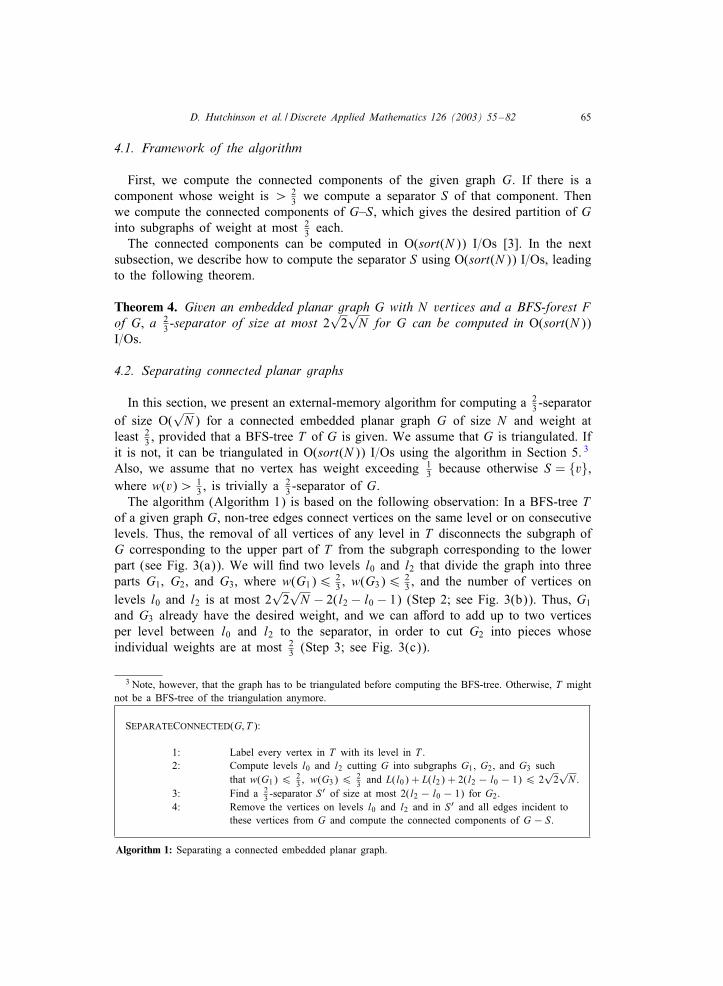
4.1. Framework of the algorithm
First, we compute the connected components of the given graph G. If there is acomponent whose weight is ¿ 2
3 we compute a separator S of that component. Thenwe compute the connected components of G–S, which gives the desired partition of Ginto subgraphs of weight at most 2
3 each.The connected components can be computed in O(sort(N )) I=Os [3]. In the next
subsection, we describe how to compute the separator S using O(sort(N )) I=Os, leadingto the following theorem.
Theorem 4. Given an embedded planar graph G with N vertices and a BFS-forest Fof G; a 2
3 -separator of size at most 2√2√
N for G can be computed in O(sort(N ))I=Os.
4.2. Separating connected planar graphs
In this section, we present an external-memory algorithm for computing a 23 -separator
of size O(√
N ) for a connected embedded planar graph G of size N and weight atleast 2
3 , provided that a BFS-tree T of G is given. We assume that G is triangulated. Ifit is not, it can be triangulated in O(sort(N )) I=Os using the algorithm in Section 5. 3
Also, we assume that no vertex has weight exceeding 13 because otherwise S = {v},
where w(v)¿ 13 , is trivially a 2
3 -separator of G.The algorithm (Algorithm 1) is based on the following observation: In a BFS-tree T
of a given graph G, non-tree edges connect vertices on the same level or on consecutivelevels. Thus, the removal of all vertices of any level in T disconnects the subgraph ofG corresponding to the upper part of T from the subgraph corresponding to the lowerpart (see Fig. 3(a)). We will 8nd two levels l0 and l2 that divide the graph into threeparts G1; G2, and G3, where w(G1)6 2
3 , w(G3)6 23 , and the number of vertices on
levels l0 and l2 is at most 2√2√
N − 2(l2 − l0 − 1) (Step 2; see Fig. 3(b)). Thus, G1
and G3 already have the desired weight, and we can aPord to add up to two verticesper level between l0 and l2 to the separator, in order to cut G2 into pieces whoseindividual weights are at most 2
3 (Step 3; see Fig. 3(c)).
3 Note, however, that the graph has to be triangulated before computing the BFS-tree. Otherwise, T mightnot be a BFS-tree of the triangulation anymore.
SEPARATECONNECTED(G; T ):
1: Label every vertex in T with its level in T .2: Compute levels l0 and l2 cutting G into subgraphs G1, G2, and G3 such
that w(G1)6 23 ; w(G3)6 2
3 and L(l0) + L(l2) + 2(l2 − l0 − 1)6 2√2√
N .3: Find a 2
3 -separator S′ of size at most 2(l2 − l0 − 1) for G2.4: Remove the vertices on levels l0 and l2 and in S′ and all edges incident to
these vertices from G and compute the connected components of G − S.
Algorithm 1: Separating a connected embedded planar graph.

66 D. Hutchinson et al. / Discrete Applied Mathematics 126 (2003) 55–82
Fig. 3. Illustrating the three major steps of the separator algorithm.
Lemma 5. Algorithm 1 computes a 23 -separator S of size at most 2
√2√
N for anembedded connected planar graph G with N vertices in O(sort(N )) I=Os; providedthat a BFS-tree of G is given.
Proof. First; let us assume that Step 3 computes the desired separator of G2 in O(sort(N )) I=Os. Then the major diIculty in Algorithm 1 is 8nding the two levels l0 and l2in Step 2. For a given level l; let L(l) be the number of vertices on level l and W (l)be the weight of the vertices on level l. We 8rst compute the level l1 closest to theroot such that
∑l6l1 W (l)¿ 1
2 (see Fig. 3(a)). Let K =∑
l6l1 L(l). Then we computelevels l06 l1 and l2 ¿ l1 such that L(l0) + 2(l1 − l0)6 2
√K and L(l2) + 2(l2 − l1 −
1)6 2√
N − K (see Fig. 3(b)). The existence of level l1 is obvious. The existence oflevels l0 and l2 has been shown in [17]. It is easy to see that levels l0 and l2 havethe desired properties.Now we turn to the correctness of Step 3. In this step, we shrink levels 0 through
l0 to a single root vertex r of weight 0. Next, we remove levels l2 and below, andretriangulate the resulting graph, obtaining a triangulation G′ (see Fig. 3(c)). Then weuse the techniques of Section 4.3 to compute a fundamental cycle C of G′ which isa 2
3 -separator of G′. Graph G2 is a subgraph of G′. Thus, G2 ∩ C is a 23 -separator of
G2. The fundamental cycle can have length at most 2(l2 − l0) − 1. If the length isindeed 2(l2 − l0) − 1, C contains the root vertex r, which is not part of G2. Thus,S ′=G2∩C has size at most 2(l2− l0−1), as desired. When shrinking levels 0 throughl0 to a single vertex we have to be a bit careful because we have to maintain theembedding of the graph. To do this we number the vertices of T lexicographicallyand sort the vertices v1; : : : ; vk on level l0 + 1 by increasing numbers (i.e., from left toright). Let wi be the parent of vi on level l0. Then, we replace edge {vi; wi} by edge{r; vi} and assign nvi({r; vi})=nvi({vi; wi}) and nr({r; vi})= i. This places edges {r; vi}counterclockwise around r and guarantees that edge {r; vi} is embedded between theappropriate edges incident to vi. We construct a BFS-tree T ′ of G′ by adding the edges{r; vi} to the remains of T in G′. It is easily veri8ed that T ′ is a spanning tree of G′.It is not so easy to see that T ′ is a BFS-tree of G′, which is crucial for simplifyingAlgorithm 2 in Section 4.3, which computes the desired separator for G′ and thus G2.
Consider the embedding of G in the plane (see Fig. 4(a)). Then, we de8ne Rl0 tobe the union of triangles that have at least one vertex at level l0 or above in T (theouter face in Fig. 4(a)). Analogously, we de8ne Rl2 to be the union of triangles that

D. Hutchinson et al. / Discrete Applied Mathematics 126 (2003) 55–82 67
Fig. 4. (a) An embedding of a given graph G. Regions Rl0 ; Rl2 , and R′ are the white, light gray, and darkgray parts of the plane, respectively. The additional curves in region Rl0 are level l0 + 1 vertices. (b) InStep 3 of Algorithm 1, we replace the graph in region Rl0 by a single root vertex r and connect it to allvertices at level l0 + 1 (dotted curves). We also remove the interior of region Rl2 . All non-triangular faceslike face f have to be triangulated.
have at least one vertex at level l2 or below in T (the light gray interior faces in Fig.4(a)). The embedding of G2 then lies in R′=R2 \ (Rl0 ∪Rl2 ) (the dark gray regions inFig. 4(a)). The boundary of R′ is a set of edge-disjoint cycles, and the interior of R′
is triangulated. Also, note that no vertex at level at most l0 can be on the boundarybetween Rl0 and R′ because all incident triangles are in Rl0 . On the other hand, for avertex at level at least l0 + 2 to be on that boundary it has to be on the boundary of atriangle that has a vertex at level at most l0 on its boundary, which is also impossible.Thus, the boundary between Rl0 and R′ is formed by level l0 + 1 vertices only. (Notethat some level l0 +1 vertices are interior to Rl0 (the additional curves in region Rl0 inFig. 4(a)).) Analogously, the boundary between Rl2 and R′ is formed by level l2 − 1vertices only. When shrinking the vertices above and including level l0 to a single rootvertex, we can think of this as removing the parts of G in Rl0 and placing the new rootvertex r into Rl0 (see Fig. 4(b)). The tree edges connecting r to level l0 + 1 verticesare embedded in Rl0 . As we did not alter the triangulation of R′ (i.e., G2), the onlyfaces of G′ where the triangulation algorithm adds diagonals are in Rl0 or Rl2 . As allvertices on the boundary of Rl0 are already connected to r, the triangulation algorithmonly adds edges connecting two level l0 + 1 or two level l2 − 1 vertices, thereby notdestroying the BFS-property of T ′ with respect to G′.Now, we analyze the complexity of Algorithm 1. Step 1 takes O(sort(N )) I=Os (see
Section 2.2). In Step 2, we sort the vertices by their levels and scan it until the totalweight of the vertices seen so far exceeds 1
2 . We continue the scan until we reachthe end of a level. While scanning we maintain the count K of visited vertices. Wescan the vertex list backward, starting at l1, and count the number of vertices on eachvisited level. When we 8nd a level l0 with L(l0)+2(l1− l0)
√K we stop. In the same
way we 8nd l2 scanning forward, starting at the level following l1. As we sort andscan a constant number of times, Step 2 takes O(sort(N )) I=Os. Removing all levels

68 D. Hutchinson et al. / Discrete Applied Mathematics 126 (2003) 55–82
Fig. 5. A non-tree edge e and the corresponding fundamental cycle C(e) shown in bold. R1(e) is the regioninside the cycle and R2(e) is the region outside the cycle.
below and including l2 takes O(sort(N )) I=Os: We sort the vertex set and 8rst sort theedges by their 8rst endpoints; in a single scan we mark all edges that have their 8rstendpoint on level l2 or below; after sorting the edges by their second endpoints, wescan the edge list again to mark all edges with their second endpoints on level l2 orbelow; 8nally, it takes a single scan to remove all marked vertices and edges. Shrinkinglevels 0 through l0 to a single root vertex takes O(sort(N )) I=Os: O(sort(N )) I=Osto number the vertices lexicographically, O(sort(N )) I=Os to sort the vertices on levell0 + 1 and another scan to replace edges {vi; wi} by edges {r; vi}. By Theorem 7, wecan retriangulate the resulting graph in O(sort(N )) I=Os. The removal of the verticesand edges in G1 can be done in a similar way as for G3. The rest of Step 3 takesO(sort(N )) I=Os by Lemma 6. Steps 2 and 3 have marked the vertices on levels l0 andl2 and in S ′ as separator vertices. Then we use the same technique as for removingG3 to remove all separator vertices and incident edges in O(sort(N )) I=Os. Computingthe connected components of G − S takes O(sort(N )) I=Os [3].
4.3. Finding a small simple cycle separator
Let G′ be the triangulation as constructed at the beginning of Step 3 of Algorithm1 and T ′ be the BFS-tree of G′ constructed from T . Every non-tree edge e = {v; w}in G′ de8nes a fundamental cycle C(e) consisting of e itself and the two paths inthe tree T ′ from the vertices v and w to the lowest common ancestor u of v and w(see Fig. 5). (Note that in a BFS-tree, u is distinct from both v and w.) Given anembedding of G′, any fundamental cycle C(e) separates G′ into two subgraphs R1(e)and R2(e), one induced by the vertices embedded inside C(e) and the other induced bythose embedded outside. In [17] it is shown that there is a non-tree edge e in G′ suchthat R1(e) and R2(e) have weights at most 2
3 each, provided that no vertex has weightexceeding 1
3 and G′ is triangulated. Moreover, for any non-tree edge e, the number ofvertices on the fundamental cycle C(e) is at most 2height(T ′) − 1 = 2(l2 − l0) − 1.Next, we show how to 8nd such an edge and the corresponding fundamental cycleI=O-eIciently.

D. Hutchinson et al. / Discrete Applied Mathematics 126 (2003) 55–82 69
We compute labels for the non-tree edges of G′ so that we can compute the weightsw(R1(e)) and w(R2(e)) of regions R1(e) and R2(e) only using the labels stored withedge e. Then we can 8nd the edge e whose corresponding fundamental cycle is a23 -separator in a single scan over the edge set of G′.Consider Fig. 5. Given a lexicographical numbering of the vertices in T ′, denote the
number assigned to vertex x by nl(x). For a given edge e={v; w}, we denote by v theendpoint with smaller lexicographical number, i.e., nl(v)¡ nl(w). Then the vertices inthe white and striped subtrees and on the path from u to w are exactly the verticeswith lexicographical numbers between nl(v) and nl(w). We compute for every vertexx a label 3l(x) =
∑nl(y)6nl(x) w(y). Then the weight of the vertices in the white and
striped subtrees and on the path from u to w is 3l(w)− 3l(v). Given for every vertexx the weight 4(x) of the vertices on the path from x, inclusive, to the root r of T ′, theweight of the vertices on the path from u to w, including w but not u, is 4(w)− 4(u),and the weight of the white and striped subtrees is 3l(w) − 3l(v) + 4(w) − 4(u). Itremains to add the weight of the cross-hatched trees and to subtract the weight of thewhite trees to obtain the weight w(R1(e)) of region R1(e).
For every edge e, we compute a label �(e). If e = {v; w} is a tree edge and v isfurther away from the root of T ′ than w, then �(e) is the weight of the subtree ofT ′ rooted at v. If e is a non-tree edge, �(e) = 0. Let e0; : : : ; ek be the list of edgesincident to a vertex x, sorted counterclockwise around x and so that e0 = {x; p(x)},where p(x) denotes x’s parent in T ′. Then we de8ne �x(e0)=0 and �x(ei)=
∑ij=1 �(ej)
for i ¿ 0. Now the weight of the white subtrees in Fig. 5 is �v(e), and the weight ofthe cross-hatched subtrees is �w(e). Thus, we can compute the weight of region R1(e)as
w(R1(e)) = 3l(w)− 3l(v) + 4(w)− 4(u) + �w(e)− �v(e): (5)
It is easy to see that the weight of region R2(e) is
w(R2(e)) = w(G′)− w(R1(e))− 4(v)− 4(w) + 24(u)− w(u) (6)
(the weight of the whole graph minus the weight of the interior region minus theweight of the fundamental cycle). Assuming that all these labels are stored with e, wecan scan the edge set of G′ and compute for every visited non-tree edge the weightsof R1(e) and R2(e) using Eqs. (5) and (6). It remains to show how to compute theselabels. We provide the details in the proof of the following lemma.
CYCLESEPARATOR(G′; T ′):
1: Compute the vertex and edge labels required to compute the weights ofregions R1(e) and R2(e), for every non-tree edge e.
a: Label every vertex x in G′ with a tuple A(x) = (W (x); nl(x); 4(x); 3l(x)),
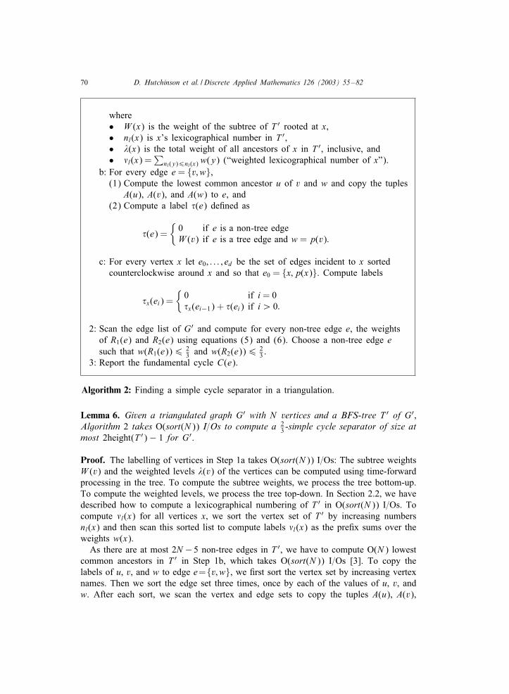
70 D. Hutchinson et al. / Discrete Applied Mathematics 126 (2003) 55–82
where• W (x) is the weight of the subtree of T ′ rooted at x,• nl(x) is x’s lexicographical number in T ′,• 4(x) is the total weight of all ancestors of x in T ′, inclusive, and• 3l(x) =
∑nl(y)6nl(x) w(y) (“weighted lexicographical number of x”).
b: For every edge e = {v; w},(1) Compute the lowest common ancestor u of v and w and copy the tuples
A(u), A(v), and A(w) to e, and(2) Compute a label �(e) de8ned as
�(e) ={0 if e is a non-tree edgeW (v) if e is a tree edge and w = p(v):
c: For every vertex x let e0; : : : ; ed be the set of edges incident to x sortedcounterclockwise around x and so that e0 = {x; p(x)}. Compute labels
�x(ei) ={0 if i = 0�x(ei−1) + �(ei) if i ¿ 0:
2: Scan the edge list of G′ and compute for every non-tree edge e, the weightsof R1(e) and R2(e) using equations (5) and (6). Choose a non-tree edge esuch that w(R1(e))6 2
3 and w(R2(e))6 23 .
3: Report the fundamental cycle C(e).
Algorithm 2: Finding a simple cycle separator in a triangulation.
Lemma 6. Given a triangulated graph G′ with N vertices and a BFS-tree T ′ of G′;Algorithm 2 takes O(sort(N )) I=Os to compute a 2
3 -simple cycle separator of size atmost 2height(T ′)− 1 for G′.
Proof. The labelling of vertices in Step 1a takes O(sort(N )) I=Os: The subtree weightsW (v) and the weighted levels 4(v) of the vertices can be computed using time-forwardprocessing in the tree. To compute the subtree weights; we process the tree bottom-up.To compute the weighted levels; we process the tree top-down. In Section 2.2; we havedescribed how to compute a lexicographical numbering of T ′ in O(sort(N )) I=Os. Tocompute 3l(x) for all vertices x; we sort the vertex set of T ′ by increasing numbersnl(x) and then scan this sorted list to compute labels 3l(x) as the pre8x sums over theweights w(x).As there are at most 2N −5 non-tree edges in T ′, we have to compute O(N ) lowest
common ancestors in T ′ in Step 1b, which takes O(sort(N )) I=Os [3]. To copy thelabels of u, v, and w to edge e={v; w}, we 8rst sort the vertex set by increasing vertexnames. Then we sort the edge set three times, once by each of the values of u, v, andw. After each sort, we scan the vertex and edge sets to copy the tuples A(u), A(v),

D. Hutchinson et al. / Discrete Applied Mathematics 126 (2003) 55–82 71
and A(w), respectively, to the edges. Computing labels �(e) then takes an additionalscan over the edge set of T ′.To compute labels �x(e) in Step 1c, we create a list L1 containing two tuples
(v; nv(e); p(v); w; �(e)) and (w; nw(e); p(w); v; �(e)) for every edge e = {v; w}. We sortthis list lexicographically, so that (the tuples corresponding to) the edges incident tovertex x are stored consecutively, sorted counterclockwise around x. Then we scan L1
and compute a list L2 of triples (v; w; �v(e)) and (v; w; �w(e)). Note that in L1, the edge(x; p(x)) is not necessarily stored as the 8rst edge in the sublist of edges incident tox causing us to skip some edges at the beginning of the sublist until we 8nd edge(x; p(x)) in the list. The skipped edges have to be appended at the end of the sublist.We can use a queue to do this. After sorting L2 as well as the edge list of T ′, it takesa single scan of the two sorted lists to copy the labels �v(e) and �w(e) to all edges e.Step 2 searches for a non-tree edge whose corresponding fundamental cycle is a
23 -separator. As already observed, this search takes a single scan over the edge list ofG′, using the labels computed in Step 1 to compute the weights w(R1(e)) and w(R2(e))of the interior and exterior regions.Step 3 is based on the following observation: Given a lexicographical numbering
nl(x) of the vertices of T ′, this numbering is also a preorder numbering. Given a vertexv with preorder number x, let the subtree rooted at v have size m. Then the vertices inthis subtree have preorder numbers x through x+m− 1. This implies that the ancestorof a vertex v at a given level l is the vertex u such that nl(u)=max{nl(u′): l(u′)= l∧nl(u′)6 nl(v)}, where l(x) denotes the level of vertex x. Using this observation we sortthe vertices by increasing levels in T ′ and in each level by increasing lexicographicalnumbers and scan this sorted list of vertices backward, 8nding the ancestors of v andw at every level until we come to a level where v and w have the same ancestor, u.Thus, Step 3 also takes O(sort(N )) I=Os.
5. Triangulating embedded planar graphs
In this section, we present an O(sort(N ))-algorithm to triangulate a connected em-bedded planar graph G = (V; E). We assume the same representation of G and itsembedding as in the previous section. Our algorithm consists of two phases. First, weidentify the faces of G. We represent each face f by a list of vertices on its bound-ary, sorted clockwise around the face. In the second phase we use this information totriangulate the faces of G. We show the following theorem.
Theorem 7. Given an embedded planar graph G; it can be triangulated in O(sort(N ))I=Os.
Proof. This follows from Lemmas 8 and 11.
5.1. Identifying faces
As mentioned above, we represent each face f by the list of vertices on its boundary,sorted clockwise around the face. Denote this list by Ff. Let F be the concatenation of

72 D. Hutchinson et al. / Discrete Applied Mathematics 126 (2003) 55–82
Fig. 6. (a) The directed graph D (dotted arrows) corresponding to a given graph G (solid lines). Note thatvertex v appears twice on the boundary of face f, and vertex w appears twice on the boundary of the outerface. (b) The directed graph G (white vertices and dotted arrows) corresponding to D.
the lists Ff for all faces f of G. The goal of the 8rst step is to compute F . The idea ofthis step is to replace every edge {v; w} of G by two directed edges (v; w) and (w; v)and decompose the resulting directed graph, D, into directed cycles, each representingthe clockwise traversal of a face of G (see Fig. 6(a)). (“Clockwise” means that wewalk along the boundary of the face with the boundary to our left. Thus, a clockwisetraversal of the outer face corresponds to walking counterclockwise along the outerboundary of the graph. This somewhat confusing situation is resolved if we imaginethe graph to be embedded on a sphere because then all faces are interior.) Removingone edge from each of these cycles gives us a set of paths. The vertices on such apath appear in the same order on the path as clockwise around the face representedby the path. (Note that the same vertex may appear more than once on the boundaryof the same face, if it is a cutpoint (see Fig. 6(a)).) Considering the set of paths as aset of lists, we can rank the lists. This gives us the orders of the vertices around allfaces, i.e., the lists Ff.The problem with the directed cycles in D is that they are not vertex-disjoint. Hence,
we cannot apply standard graph external-memory algorithms to extract these cycles.The following modi8cation solves this problem: Instead of building D, we build agraph G for G (see Fig. 6(b)), which is closely related to the representation of Gby a doubly-connected edge list [21]. G contains a vertex v(v;w) for every edge (v; w)in D and an edge between two vertices v(u;v) and v(v;w) if the corresponding edges(u; v) and (v; w) are consecutive in some cycle of D representing a face of G. GraphG consists of vertex-disjoint cycles, each representing a face of G. We compute theconnected components of G, thereby identifying the cycles of G, and apply the sametransformations to G that we wanted to apply to D. Step 1 of Algorithm 3 gives thedetails of the construction of G. In Step 2, we use G to compute F .
Lemma 8. Algorithm 3 takes O(sort(N )) I=Os to constructs the list F for a givengraph G.
D. Hutchinson et al. / Discrete Applied Mathematics 126 (2003) 55–82 73
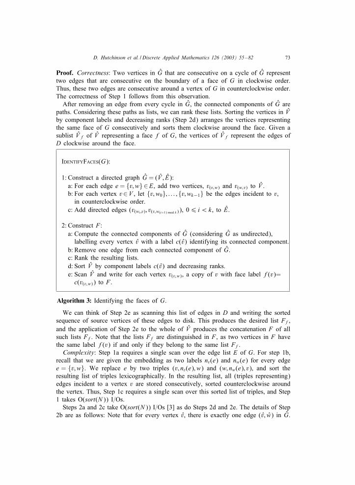
Proof. Correctness: Two vertices in G that are consecutive on a cycle of G representtwo edges that are consecutive on the boundary of a face of G in clockwise order.Thus; these two edges are consecutive around a vertex of G in counterclockwise order.The correctness of Step 1 follows from this observation.After removing an edge from every cycle in G, the connected components of G are
paths. Considering these paths as lists, we can rank these lists. Sorting the vertices in Vby component labels and decreasing ranks (Step 2d) arranges the vertices representingthe same face of G consecutively and sorts them clockwise around the face. Given asublist V f of V representing a face f of G, the vertices of V f represent the edges ofD clockwise around the face.
IDENTIFYFACES(G):
1: Construct a directed graph G = (V ; E):a: For each edge e = {v; w}∈E, add two vertices, v(v;w) and v(w;v) to V .b: For each vertex v∈V , let {v; w0}; : : : ; {v; wk−1} be the edges incident to v,in counterclockwise order.
c: Add directed edges (v(wi;v); v(v;w(i+1) mod k )), 06 i ¡ k, to E.
2: Construct F :a: Compute the connected components of G (considering G as undirected),labelling every vertex v with a label c(v) identifying its connected component.
b: Remove one edge from each connected component of G.c: Rank the resulting lists.d: Sort V by component labels c(v) and decreasing ranks.e: Scan V and write for each vertex v(v;w), a copy of v with face label f(v)=
c(v(v;w)) to F .
Algorithm 3: Identifying the faces of G.
We can think of Step 2e as scanning this list of edges in D and writing the sortedsequence of source vertices of these edges to disk. This produces the desired list Ff,and the application of Step 2e to the whole of V produces the concatenation F of allsuch lists Ff. Note that the lists Ff are distinguished in F , as two vertices in F havethe same label f(v) if and only if they belong to the same list Ff.
Complexity: Step 1a requires a single scan over the edge list E of G. For step 1b,recall that we are given the embedding as two labels nv(e) and nw(e) for every edgee = {v; w}. We replace e by two triples (v; nv(e); w) and (w; nw(e); v), and sort theresulting list of triples lexicographically. In the resulting list, all (triples representing)edges incident to a vertex v are stored consecutively, sorted counterclockwise aroundthe vertex. Thus, Step 1c requires a single scan over this sorted list of triples, and Step1 takes O(sort(N )) I=Os.Steps 2a and 2c take O(sort(N )) I=Os [3] as do Steps 2d and 2e. The details of Step
2b are as follows: Note that for every vertex v, there is exactly one edge (v; w) in G.

74 D. Hutchinson et al. / Discrete Applied Mathematics 126 (2003) 55–82
Thus, we sort V by vertex names and E by the names of the source vertices, therebyplacing edge (v; w) at the same position in E as v’s position in V . Scanning V and Esimultaneously, we assign component labels c((v; w)) = c(v) to all edges (v; w) in E.Then we sort E by these component labels. Finally we scan E again and remove everyedge whose component label is diPerent from the component label of the previousedge. Also, we remove the 8rst edge in E. As this procedure requires sorting andscanning V and E twice, the complexity of Step 2 is O(sort(N )) I=Os.
5.2. Triangulating faces
We triangulate each face f in four steps (see Algorithm 4). In Step 1, we reduce fto a simple face f. That is, no vertex appears more than once in a clockwise traversalof f’s boundary. Accordingly, we reduce the list Ff to Ff. In Step 2, we triangulate
f. We guarantee that there are no parallel edges in f. But we may add parallel edgesto diPerent faces (see Fig. 8(a) for an example). Let e1; : : : ; ek be the set of edges withendpoints v and w. In Step 3, we select one of these edges, say e1, and mark edgese2; : : : ; ek as con=icting. Each of these edges is said to be in con=ict with e1. In Step4, we retriangulate all faces so that conGicts are resolved and a 8nal triangulation isobtained.The following lemma states the correctness of Step 1.
Lemma 9. For each face f of G; the face f computed by Step 1 of Algorithm 4 issimple. The parts of f that are not in f are triangulated. Moreover; Step 1 doesnot introduce parallel edges.
Proof. We mark exactly one copy of every vertex on f’s boundary. For the 8rst vertex;we append a second marked copy to the end of Ff only to close the cycle. This copyis removed at the end of Step 1. We remove an unmarked vertex v by adding an edgebetween its predecessor u and successor w on the current boundary of the face; therebycutting triangle (u; v; w) oP the boundary of f. As we remove all unmarked verticesthis way; the resulting face f is simple and the parts that have been removed from fto produce f are triangulated.Next, we show that Step 1 does not add parallel edges to the same face f. Assume
for the sake of contradiction that we have added two edges with
TRIANGULATEFACES(G; F):
1: Make all faces of G simple:
For each face f, (a) mark the 8rst appearance of each vertex v in Ff, (b)append a marked copy of the 8rst vertex in Ff to the end of Ff, (c) scanFf backward and remove each unmarked vertex v from f and Ff by addinga diagonal between its predecessor and successor in the current list, and (d)remove the last vertex from list Ff. Call the resulting list Ff.

D. Hutchinson et al. / Discrete Applied Mathematics 126 (2003) 55–82 75
2: Triangulate the simple faces:Let Ff = 〈v0; : : : ; vk〉. Then add “temporary diagonals” {v0; vi}, 26 i6 k − 1,to f.
3: Mark conGicting diagonals:Sort E lexicographically, representing edge {v; w} by an ordered pair (v; w),v ¡ w, and so that edge {v; w} is stored before any “temporary diagonal”{v; w}. Scan E and mark all occurrences except the 8rst of each edge asconGicting. Restore the original order of all edges and “temporary diagonals”.
4: Retriangulate conGicting faces:a: For each face f, let Df = 〈{v0; v2}; : : : ; {v0; vk−1}〉 be the list of “temporarydiagonals”.
b: Scan Df until we 8nd the 8rst conGicting diagonal {v0; vi}.c: Replace the diagonals {v0; vi}; : : : ; {v0; vk−1} by new diagonals{vi−1; vi+1}; : : : ; {vi−1; vk}.
Algorithm 4: Triangulating the faces of G.endpoints v and w to f (see Fig. 7(a)). We can add two such edges e1 and e2 onlyif one of the endpoints, say w, appears at least twice in a clockwise traversal off’s boundary. Then, however, there is at least one vertex x that has all its occurrencesbetween two consecutive occurrences of w because e1 and e2 form a closed curve. Thatis, the marked copy of x also appears between these two occurrences of w. Addinge2 to f would remove this marked copy from f’s boundary; but we never removemarked vertices. Thus, e2 cannot exist.Now assume that we add two edges e1 and e2 with endpoints v and w to diPerent
faces f1 and f2. By adding e1 we remove a vertex u from f1’s boundary (see Fig.7(b)). As this copy is unmarked, there has to be another, marked, copy of u. Considerthe region R1 enclosed by the curve between the marked copy of u and the removedcopy of u, following the boundary of f1. In the same way we de8ne a region R2
enclosed by the curve between the removed copy of u and the marked copy of u.
Fig. 7. Illustrating the proof of Lemma 9.

76 D. Hutchinson et al. / Discrete Applied Mathematics 126 (2003) 55–82
Fig. 8. (a) A simple face f with a conGicting diagonal edge d = {v0; vi}. Diagonal d conGicts with d′ anddivides f into two parts f1 and f2. One of them, f1, is conGict-free. Vertex vi−1 is the third vertex ofthe triangle in f1 that has d on its boundary. (b) The conGict-free triangulation of f.
Any face other than f1 that has v on its boundary must be in R1. Any face other thanf1 that has w on its boundary must be in R2. However, R1 and R2 are disjoint. Thus,we cannot add a diagonal {v; w} to any face other than f1.
Step 2 triangulates all simple faces f, possibly adding parallel edges to diPerentfaces. Consider all edges e1; : : : ; ek with endpoints v and w. We have to remove atleast k − 1 of them. Also, if edge {v; w} was already in G, we have to keep this edgeand remove all diagonals that we have added later. That is, the edge {v; w} is the edgewith which all diagonals {v; w} are in conGict, and we have to label all diagonals asconGicting while labelling edge {v; w} as non-conGicting. If edge {v; w} was not inG, we can choose an arbitrary diagonal {v; w} with which all other diagonals with thesame endpoints are in conGict. This strategy is realized in Step 3. The following lemmastates the correctness of Step 4, thereby 8nishing the correctness proof for Algorithm4.
Lemma 10. Step 4 makes all faces f con=ict-free; i.e.; the triangulation obtainedafter Step 4 does not contain parallel edges.
Proof. Let d={v0; vi} be the edge found in Step 4b (see Fig. 8(a)). Then d cuts f intotwo halves, f1 and f2. All diagonals {v0; vj}, j ¡ i are in f1; all diagonals {v0; vj},j ¿ i are in f2. That is, f1 does not contain conGicting diagonals. Vertex vi−1 is thethird vertex of the triangle in f1 that has d on its boundary. Step 4c removes d andall edges in f2 and retriangulates f2 with diagonals that have vi−1 as one endpoint.(Intuitively it forms a star at the vertex vi−1; see Fig. 8(b).)Let d′ be the edge that d is in conGict with. Then d and d′ form a closed curve.
Vertex vi−1 is outside this curve and all boundary vertices of f2 excluding the endpointsof d are inside this curve. As we keep d′, no diagonal, except for the new diagonalsin f, can intersect this curve. Thus, the new diagonals in f are non-conGicting. The“old” diagonals in f were in f1 and thus, by the choice of d and f1, non-conGicting.Hence, f does not contain conGicting diagonals.

D. Hutchinson et al. / Discrete Applied Mathematics 126 (2003) 55–82 77
Lemma 11. Given the list F as computed by Algorithm 3; Algorithm 4 triangulatesthe given graph G in O(sort(N )) I=Os.
Proof. We have already shown the correctness of Algorithm 4. In Step 1; we 8rstsort every list Ff by vertex names. Then it takes a single scan to mark the 8rstoccurrences of all vertices in Ff. Using another sort we restore the original order ofthe vertices in Ff. The rest of Step 1 requires scanning F; writing the marked verticesto Ff; in their order of appearance; and keeping the last visited marked vertex in mainmemory in order to add the next diagonal. Thus; Step 1 takes O(sort(N )) I=Os. Step2 requires a single scan over the list F; as modi8ed by Step 1. Assuming that alledges in G before the execution of Step 2 were labelled as “edges”; we label all edgesadded in Step 2 as “diagonals”. Then Step 3 requires sorting the list of edges anddiagonals lexicographically and scanning this sorted list to label conGicting diagonals.Note; however; that Step 4 requires the diagonals to be stored in the same order asadded in Step 2. Thus; before sorting in Step 3; we label every edge with its currentposition in E. At the end of Step 3; we sort the edges by these position labels torestore the previous order of the edges. Of course; Step 3 still takes O(sort(N )) I=Os.Step 4 takes a single scan over E. Thus; the whole algorithm takes O(sort(N )) I=Os.
A problem that we have ignored so far is embedding the new diagonals. Next, wedescribe how to augment Algorithm 4 in order to maintain an embedding of G underthe edge insertions performed by the algorithm. To do this, we have to modify therepresentation of the embedding slightly. Initially, we assumed that the edges e1; : : : ; ek
incident to a vertex v are assigned labels nv(ei) = i clockwise around v. During thetriangulation process we allow labels nv(e) that are multiples of 1=N . Note that thisdoes not cause precision problems because we can represent every label nv(e) as aninteger N · nv(e) using at most 2 logN bits (while nv(e) uses logN bits).Let v0; e0; v1; e1; : : : ; vk−1; ek−1 be the list of vertices and edges visited in a clockwise
traversal of the boundary of a face f (i.e., Ff=〈v0; : : : ; vk−1〉). During the constructionof Ff, we can easily assign labels n1(vi) and n2(vi) to the vertices, where n1(vi) =nvi(e(i−1) mod k) and n2(vi) = nvi(ei). When we add a diagonal d = {vi; vj}, i ¡ j, weupdate the labels of vi and vj to n2(vi)=n2(vi)−1=N and n1(vj)=n1(vj)+1=N and embedd assigning nvi(d) = n2(vi) and nvj (d) = n1(vj). Assuming that n1(vi)¡ n2(vi) − 1=Nor n1(vi)¿ n2(vi) and n2(vj)¿ n1(vj)+1=N or n2(vj)6 n1(vj), this embeds d betweene(i−1) mod k and ei at vi’s end and e(j−1) mod k and ej at vj’s end. It remains to show thatthis assumption is always satis8ed.We maintain the following invariant for every face f: Let v0; e0; : : : ; vk−1; ek−1 be
the boundary description of f as given above. Then for every vertex vi, either n1(vi)+(k − 3)=N ¡ n2(vi) or n1(vi)¿ n2(vi). Initially, this is true because all labels nv(e) areintegers and k6N . Adding diagonal d to f as above cuts f into two faces f1 and f2.For all vertices vl, l �∈ {i; j}, the labels do not change; but the sizes of f1 and f2 areless than the size of f. Thus, for all these vertices the invariant holds. We show thatthe invariant holds for vi. A similar argument can be applied for vj. Let f1 be the facewith vertices vj; : : : ; vi on its boundary and f2 be the face with vertices vi and vj on the

78 D. Hutchinson et al. / Discrete Applied Mathematics 126 (2003) 55–82
Fig. 9. A given planar graph G (a) and its separator tree ST (G) (b). Note that any path between verticesv and w, which are stored in the white and gray subtrees of ST (G), respectively, must contain a black orhorizontally striped separator vertex. These separators are stored at common ancestors of 5(v) and 5(w).
boundary. Let the size of fi be ki6 k−1. If n2(vi)6 n1(vi), then this is also true aftersubtracting 1=N from n2(vi). Otherwise, n2(vi)−n1(vi)¿ (k−3)=N −1=N ¿ (k1−3)=N .Thus, the invariant holds for all vertices on f1’s boundary. In f2 we do not have anyroom left to add diagonals incident to vi or vj. However, Steps 1 and 4 of Algorithm4 scan along the boundaries of the faces and keep cutting oP triangles. Choosing theindices i and j in the above description so that f2 is the triangle that we cut oP, wenever add another diagonal to f2. (Note that it would be just as easy to maintain theembedding in Step 2; but we need not even do this because diagonals are added onlytemporarily in Step 2, and 8nal diagonals are added in Step 4.)
6. The shortest path data structure
In this section, we incorporate the main ideas of the internal memory shortest pathdata structure in [8] and show how to use them together with the external-memorytechniques developed in this paper to design an eIcient external-memory shortest pathdata structure. The data structure in [8] uses O(S) space and answers distance queries ongraphs with separators of size O(
√N ) in O(N 2=S) time, where 16 S6N 2. Reporting
the corresponding shortest path takes O(K) time, where K is the number of verticeson the path. The basic structure used to obtain the above trade-oP is an O(N 3=2)size internal memory data structure that answers distance queries in O(
√N ) time. Our
external-memory data structure is fully blocked. That is, it uses O(N 3=2=B) blocks ofexternal memory and answers distance queries in O(
√N=DB) I=Os. The corresponding
shortest path can be reported in O(K=DB) I=Os.Given a planar graph G (see Fig. 9(a)), we compute a separator tree ST (G) for
G (see Fig. 9(b)). This tree is de8ned recursively: We compute a 23 -separator S(6)
of size O(√|G|) for G. Let G1; : : : ; Gk be the connected components of G–S(6).
Then we store S(6) at the root 6 of ST (G) and recursively build separator treesST (G1); : : : ; ST (Gk), whose roots become the children of 6. Thus, every vertex vof G is stored at exactly one node 5(v)∈ ST (G). For two vertices v and w, let

D. Hutchinson et al. / Discrete Applied Mathematics 126 (2003) 55–82 79
5(v; w)=lca(5(v); 5(w)). For a vertex 5∈ ST (G), we de8ne S−(5) (resp. S+(5)) as thesets of vertices stored at 5 and its ancestors (resp. descendants). For convenience, wedenote the sets S(5(v)) and S(5(v; w)) by S(v) and S(v; w), respectively. Sets S−(v),S+(v), S−(v; w) and S+(v; w) are de8ned analogously. In [8], it is shown that anypath between v and w in G must contain at least one vertex in S−(v; w). For a givengraph H , we denote the distance between two vertices v and w in H by dH (v; w).Then d(v; w) = minx∈S−(v;w){dG[S+(x)](x; v) + dG[S+(x)](x; w)}. If we represent all setsS−(v) and S−(v; w) as lists sorted by increasing depth in ST (G), then S−(v; w) is thelongest common pre8x of S−(v) and S−(w). Let D(v) be a list of distances, wherethe ith entry in D(v) is the distance dG[S+(x)](v; x) between v and the ith entry x inS−(v). Given the lists S−(v), S−(w), D(v), and D(w), we can compute d(v; w) byscanning these four lists. We scan S−(v) and S−(w) in “lock-step” fashion and testwhether xv = xw, where xv and xw are the current entries visited in the scans of thetwo lists. If xv = xw, then we proceed in the scans of D(v) and D(w) to computedG[S+(xv)](xv; v) + dG[S+(xv)](xv; w) and compare it to the previously found minimum. Ifxv �= xw, we have reached the end of S−(v; w) and stop.
For every separator vertex x, our data structure contains a shortest path tree SPT (x)with root x. This tree represents the shortest paths between x and all vertices inG[S+(x)]. That is, every vertex v of G[S+(x)] is represented by a node in SPT (x),and the shortest path from v to x in G[S+(x)] corresponds to the path from v to x inSPT (x). Given the distance d(v; w) between two vertices v and w, there must be somevertex xmin ∈ S−(v; w) such that d(v; w) = dG[S+(xmin)](xmin ; v) + dG[S+(xmin)](xmin ; w). Theshortest path &(v; w) from v to w is the concatenation of the shortest paths from v toxmin and from xmin to w. Given SPT (xmin), we can traverse the paths from v and w tothe root xmin and concatenate the traversed paths to obtain &(v; w). To traverse thesetwo paths in the tree, we have to 8nd the two (external) memory locations holding thetwo nodes representing v and w in SPT (xmin). We construct lists P(v) for all verticesv of G holding pointers to the representatives of v in all shortest path trees. Let xbe the separator vertex stored at the ith position in S−(v). Then the ith position ofP(v) holds a pointer to the node representing v in SPT (x). That is, if xmin is stored atposition i in S−(v) and S−(w), the ith positions of P(v) and P(w) hold the addressesof the representatives of v and w in SPT (xmin), giving us enough information to starttraversing and reporting &(v; w).The size of the separator S(5) stored at every vertex 5 in the separator tree ST (G)
is O(√|G[S+(5)]|). From one level in ST (G) to the next the sizes of the subgraphs
G[S+(5)] associated with the vertices decrease by a factor of at least 23 . Thus, the
sizes of the graphs G[S+(5)] on a root-to-leaf path in ST (G) are bounded from aboveby a geometrically decreasing sequence, and the sizes of the separators S(5) stored atthese vertices form a geometrically decreasing sequence as well. Hence, there are onlyO(
√N ) separator vertices on any such path and each list S−(v) has size O(
√N ). As
we have to scan lists S−(v), S−(w), D(v), and D(w) to compute d(v; w), this takesO(
√N=DB) I=Os. It takes two more I=Os to access the pointers in P(v) and P(w).
Assuming that all shortest path trees have been blocked as described in Section 3,traversing the paths from v and w to xmin in SPT (xmin) takes O(K=DB) I=Os, where Kis the number of vertices on the shortest path &(v; w).

80 D. Hutchinson et al. / Discrete Applied Mathematics 126 (2003) 55–82
It remains to show that the data structure can be stored in O(N 3=2=B) blocks. Asevery list S−(v), D(v), and P(v) has size O(
√N ) and there are 3N such lists, all lists
require O(N 3=2) space and can thus be stored in O(N 3=2=B) blocks. There is exactlyone shortest path tree for every separator vertex. Consider tree SPT (x) and a node v inthis tree. Then this node corresponds to the entry for x in list S−(v). That is, there isa one-to-one correspondence between entries in the lists S−(v) and shortest path treenodes. Thus, the total size of all shortest path trees is O(N 3=2) as well. As blockingthe shortest path trees increases the space requirements by only a constant factor, theshortest path trees can also be stored in O(N 3=2=B) blocks of external memory. Wehave shown the following theorem.
Theorem 12. Given a planar graph G with N vertices; one can construct a datastructure that answers distance queries between two vertices in G in O(
√N=DB)
I=Os. The corresponding shortest path can be reported in O(K=DB) I=Os; where Kis the length of the reported path. The data structure occupies O(N 3=2=B) blocks ofexternal memory.
7. Conclusions
The I=O-eIcient construction of our shortest path data structure is still a problem, asthere are no algorithms for BFS, embedding, and the single source shortest path problemthat perform I=O-eIciently on planar graphs. The separator algorithm in Section 4 triesto address the problem of computing the separators required to build the separator treeI=O-eIciently. Also, in [26] an O(sort(N )) algorithm for transforming a given rootedtree of size N into the blocked form described in Section 3 is given.A shortcoming of our separator algorithm is that it needs a BFS-tree. Most separator
algorithms rely on BFS, but BFS and depth-8rst search (DFS) seem to be hard problemsin external memory. Thus, it is an important open problem to develop an I=O-eIcientseparator algorithm that does not need BFS or DFS. The existence of an I=O-eIcientplanar embedding algorithm is also open.Recently, Maheshwari and Zeh [18] presented O(sort(N )) algorithms for outer-
planarity testing, computing an outerplanar embedding, BFS, DFS, and computing a23 -separator of a given outerplanar graph. It is an important question whether there areother interesting classes of graphs with similar I=O-complexities for these problems.They also showed U(perm(N )) lower bounds for computing an outerplanar embed-ding, and BFS and DFS in outerplanar graphs. As outerplanar graphs are also planar,the lower bounds for BFS and DFS also apply to planar graphs. A similar technique asin [18] can be used to show that planar embedding has an U(perm(N )) lower bound.
Acknowledgements
The authors would like to thank Lyudmil Aleksandrov, JWorg-RWudiger Sack, Hans-Dietrich Hecker, and Jana Dietel for their critical and helpful remarks.

D. Hutchinson et al. / Discrete Applied Mathematics 126 (2003) 55–82 81
References
[1] L. Aleksandrov, H. Djidjev, Linear algorithms for partitioning embedded graphs of bounded genus,SIAM J. Discrete Math. 9 (1996) 129–150.
[2] L. Arge, The buPer tree: a new technique for optimal I=O-algorithms, in: Proceedings of the Workshopon Algorithms and Data Structures, Lecture Notes in Computer Science, Vol. 955, Springer, Berlin,1995, pp. 334–345.
[3] Y.-J. Chiang, M.T. Goodrich, E.F. Grove, R. Tamassia, D.E. VengroP, J.S. Vitter, External-memorygraph algorithms, in: Proceedings of the Sixth Annual ACM-SIAM Symposium on Discrete Algorithms,January 1995.
[4] A. Crauser, K. Mehlhorn, U. Meyer, KWurzeste-Wege-Berechnung bei sehr groYen Datenmengen, in:O. Spaniol (Ed.), Promotion tut not: Innovationsmotor “Graduiertenkolleg”, Aachener BeitrWage zurInformatik, Vol. 21, Verlag der Augustinus Buchhandlung, 1997.
[5] F. Dehne, W. Dittrich, D. Hutchinson, EIcient external memory algorithms by simulating coarse-grainedparallel algorithms, in: Proceedings of the Ninth ACM Symposium on Parallel Algorithms andArchitectures, 1997, pp. 106–115.
[6] E.W. Dijkstra, A note on two problems in connection with graphs, Numer. Math. 1 (1959) 269–271.[7] K. Diks, H.N. Djidjev, O. Sykora, I. Vrto, Edge separators of planar and outerplanar graphs with
applications, J. Algorithms 14 (1993) 258–279.[8] H.N. Djidjev, EIcient algorithms for shortest path queries in planar digraphs, in: Proceedings of the
22nd Workshop on Graph-Theoretic Concepts in Computer Science, Lecture Notes in Computer Science,Springer, Berlin, 1996, pp. 151–165.
[9] G.N. Frederickson, Fast algorithms for shortest paths in planar graphs, with applications, SIAM J.Comput. 16 (6) (1987) 1004–1022.
[10] G.N. Frederickson, Planar graph decomposition and all pairs shortest paths, J. ACM 38 (1) (1991)162–204.
[11] M.L. Fredman, R.E. Tarjan, Fibonacci heaps and their uses in improved network optimization algorithms,J. ACM 34 (1987) 596–615.
[12] H. Gazit, G.L. Miller, A parallel algorithm for 8nding a separator in planar graphs, in: Proceedings ofthe 28th Symposium on Foundations of Computer Science, 1987, pp. 238–248.
[13] M.T. Goodrich, Planar separators and parallel polygon triangulation, in: Proceedings of the 24th ACMSymposium on Theory of Computing, 1992, pp. 507–516.
[14] D. Hutchinson, A. Maheshwari, N. Zeh, An external memory data structure for shortest path queries,in: Proceedings of the Fifth ACM-SIAM Computing and Combinatorics Conference, Lecture Notes inComputer Science, Vol. 1627, Springer, Berlin, July 1999, pp. 51–60.
[15] P. Klein, S. Rao, M. Rauch, S. Subramanian, Faster shortest-path algorithms for planar graphs, in:Proceedings of the 26th ACM Symposium on Theory of Computing, May 1994, pp. 27–37.
[16] M. Lanthier, A. Maheshwari, J.-R. Sack, Approximating weighted shortest paths on polyhedral surfaces,in: Proceedings of the 13th Annual ACM Symposium on Computational Geometry, June 1997, pp. 274–283.
[17] R.J. Lipton, R.E. Tarjan, A separator theorem for planar graphs, SIAM J. Appl. Math. 36 (2) (1979)177–189.
[18] A. Maheshwari, N. Zeh, External memory algorithms for outerplanar graphs, in: Proceedings of theISAAC’99, Lecture Notes in Computer Science, Springer, Berlin, December 1999, to appear.
[19] K. Munagala, A. Ranade, I=O-complexity of graph algorithms, in: Proceedings of the 10th AnnualACM-SIAM Symposium on Discrete Algorithms, January 1999.
[20] M. Nodine, M. Goodrich, J. Vitter, Blocking for external graph searching, Algorithmica 16 (2) (1996)181–214.
[21] F.P. Preparata, M.I. Shamos, Computational Geometry—An Introduction, Springer, Berlin, 1985.[22] C. Ruemmler, J. Wilkes, An introduction to disk drive modeling, IEEE Comput. 27 (3) (1994) 17–28.[23] J.S. Vitter, External memory algorithms, in: Proceedings of the 17th Annual ACM Symposium on
Principles of Database Systems, June 1998.[24] J. Vitter, E. Shriver, Algorithms for parallel memory I: two-level memories, Algorithmica 12 (2–3)
(1994) 110–147.

82 D. Hutchinson et al. / Discrete Applied Mathematics 126 (2003) 55–82
[25] J. Vitter, E. Shriver, Algorithms for parallel memory II: hierarchical multilevel memories, Algorithmica12 (2–3) (1994) 148–169.
[26] N. Zeh, An external-memory data structure for shortest path queries, Diplomarbeit, FakultWat fWurMathematik und Informatik, Friedrich-Schiller-UniversitWat Jena, November 1998.