An Exploration of the Seismograph

David Mayrhofer

Abstract

The seismograph is an instrument of extreme importance in seismology, giving invaluable informationto those studying earthquakes. The seismograph operates off of the principle of inertia, and can bedescribed essentially as a harmonic oscillator. We explore this theoretical description of the instrumentas a damped driven harmonic oscillator in case of the mass and spring, the pendulum, and the zerolength spring pendulum. We investigate the effects of the damping coefficient on the system and findthat optimal damping for the oscillator will occur between 60% and 70% of its resonance frequency.

1 Introduction

Vibrations play an important part in the natural world, being key aspects of fundamental phenomena such aslight and sound. The vibrations of the ground are of interest to many, as they arise not only from naturallyoccurring earthquakes, but can be used to determine the structure and stability of the ground far below us.Therefore, the development of an accurate seismograph is desirable, and over the course of history manyhave created devices that allowed them to detect such vibrations.

1.1 Earthquakes

In order to discuss the important traits in a seismograph, there must first be a discussion about the ba-sic features of earthquakes. Earthquakes occur when energy in the ground is released and causes suddenmovement. This happens when the tectonic plates in the Earth build up enough strain to break the surfacelayer of rock. The energy is then released in the form of waves, which are what we call earthquakes [3].Earthquakes are usually made up of four different types of waves. The wave that comes first is called theprimary or P wave. This wave is longitudinal, and travels very quickly, as it is able to travel through theEarth’s core. The second type of wave is the secondary or S wave. This is a transverse wave, and travelsmuch more slowly than the P wave. The other two types of waves are called surface waves. These can, inturn, be broken down into Rayleigh and Love waves. Love waves tend to travel faster than the Rayleighwaves, and tend to be fairly strong in amplitude. Rayleigh waves tend to spread more quickly, and as resultlast a long time when recording on a seismograph [7]. This variety of waves can each produce a relativelybroad range of frequencies and amplitutdes, as shown in Figure 1.

1.2 History

The first recorded instance of a seismograph occurred in 2nd century China, when Zhang Heng created adevice that would detect earthquakes which were too small to be felt. This seismograph was in the shapeof a cylinder, and when an earthquake would occur, a ball would fall out of the cylinder. While the exactmechanism of the device is not known, it is believed that inside the cylinder was a pendulum that wouldbegin to move when the ground shook, and would knock the ball from the cylinder. This device could notmeasure the amplitude or frequency of the earthquake, but is the first recorded attempt at detecting groundmotion that cannot be felt by humans [8].

The attempts at making a more accurate seismograph were somewhat sporadic in Europe until the 1700s.One of the earliest concepts for a seismograph was thought of by J. de la Haute Feuille, who in 1701 proposedfilling a bowl with mercury, then measuring the amount and direction of the mercury spilled to determine thedirection and amplitude of the earthquake. Ultimately though, his ideas were never implemented. Variousattempts would be made throughout the next 150 years, and in the 19th century, many important advance-ments in the field were made [5]. In 1855, Luigi Palmieri made a seismograph that could measure theamplitude of an earthquake, and in 1875 Filippo Cecchi created the first seismograph that could, in additionto tracking the amplitude of the quake, measure the vibrations over a period of time. These seismographsused pendulums to track the motion of the ground, much like in the ancient Chinese instrument [8].

In the late 19th century, a trio of European scientists in Japan made several advancements in the de-velopment of the instrument. Sir James Alfred Ewing, Thomas Gray, and John Milne worked to increasethe accuracy of the seismograph, and even founded the Seismological Society of Japan after an especiallylarge earthquake at Yokohama. One major achievement in this time was the invention of the horizontalseismograph. This seismograph operated on the principal of tracking solely the S waves of an earthquake.

1

Figure 1: A chart showing the various amplitudes and frequencies possible for different types of earthquakes[2].

It consists of a rod attached to a pivot, with a mass suspended from the end of the rod closer to the pivotand some recording device to track the motion of the rod at the other end, as can be seen in Figure 2.This design would be modified over time, but the basic aspects of this design are still used to this day [9].

1.3 Description

The seismograph functions based off of the principle of inertia. That is, an object will not accelerate unlessacted upon by an outside force. Therefore, if one could suspend a mass at equilibrium in the air withouthaving any contact with the ground, when an earthquake would occur, the mass would not move. The masswould appear to move from the perspective of the ground, and that apparent motion would be equivalent tothe actual motion of the ground. However, this is not actually feasible. Instead, we use a simple harmonicoscillator in an attempt to approximate this situation. In the case of a seismograph that detects verticalmotion, this is may be done by a mass and spring system. The mass is suspended above the ground, andwhile the ground may shift vertically, the mass will not feel a significant force until the spring has beensufficiently compressed. In a seismograph, the mass is usually chosen to be large, as this reduces the effectsof the spring on the position of the mass. Since mass and spring system is a simple harmonic oscillator,other types of simple harmonic oscillators can also be used in a seismograph. Many seismographs will use apendulum. This is especially useful when measuring the horizontal displacement of the ground.

In practice, a few other aspects of the seismograph must be considered. For instance, the device mustbe fixed in some manner so that is does not record horizontal motion if it is a vertical seismograph, or fixedso that it does not record vertical motion if it is a horizontal seismograph. The amplitudes of earthquakesare often also very small, so the motion detected by the instrument must be amplified. This is usually doneby converting the motion of the mass into an electric signal, then amplifying this signal before recordingthe results. The damping of the oscillator must also be taken into account, as this affects the relationshipbetween the motion of the ground and the motion of the oscillator. This is done by using a magnetic dampingsystem, which can adjusted to a range of different damping coefficients [4].

2

Figure 2: The horizontal seismograph as designed by Milne [8].

Figure 3: A drawing of simple horizontal and vertical seismographs with key features labelled [10].

2 The Displacement of the Mass and the Ground1

We begin by looking at the equations of motion for a simple harmonic oscillator with spring constant k,mass m, and damping coefficient b. Since this we know this force is caused by the motion of the ground, wecan then write

x(t) + 2β0x(t) + ω20x(t) = −u(t), (1)

where ω0 =√

km , β0 = b

2m , and u(t) is the motion of the ground. However, we assume that the damping

factor β0 is close to or much smaller than the resonant frequency ω0, since if it were much larger it wouldconstitute an overdamped system and would clearly interfere with the mass tracking the motion of the earth.Therefore, it is more convenient to have the ratio of β0 to ω0, so we define β = β0

ω0. Then the differential

1The derivation in this section is based on the derivations by Robert Nowack in his lecture notes for Introduction forSeismology at http://web.ics.purdue.edu/∼nowack/geos557/lecture3a-dir/lecture3a.htm and Section 12.1.1 of Aki and Richard’sQuantitative Seismology

3

equation we will be working with is

x(t) + 2βω0x(t) + ω20x(t) = −u(t), (2)

Without knowing what u(t) is, we cannot find an exact solution to (2). However, this expression can tellus a few other things about the motion of the system. For instance, we notice that when the vibrations ofthe earth are very fast compared the resonant frequency of the oscillator, the position of the mass will beproportional to the position of the ground. To get a better picture of how this equation behaves, we takethe Fourier transform of the equation to look at the corresponding equation with respect to the frequencyof the driving function ω.

X(ω) = F (x(t)) =

∫ ∞−∞

x(t)e−2πitω dω, U(ω) = F (u(t)) =

∫ ∞−∞

u(t)e−2πitω dω (3)

We note that for any function f(t), for a Fourier transform in ω we have F (f(t)) = −iωF (f(t)). So ourtransformed differential equation is

−ω2X(ω)− 2iβω0ωX(ω) + ω20X(ω) = ω2U(ω) (4)

We can rearrange this expression to obtain the ratio of the displacement of the mass and the displacementof the ground. We find that that

X(ω)

U(ω)=

ω2

ω20 − ω2 − 2iβω0ω

=ω2(ω2

0 − ω2 + 2iβω0ω)

(ω20 − ω2)2 + (2βω0ω)2

=ω2√

(ω20 − ω2)2 + (2βω0ω)2

[cos

(arctan

2βω0ω

ω20 − ω2

)+ i sin

(arctan

2βω0ω

ω20 − ω2

)]=

ω2√(ω2

0 − ω2)2 + (2βω0ω)2ei arctan

2βω0ω

ω20−ω2

(5)

From this, we can tell a little bit more about the nature of the ratio of the two functions. The ratios ofthe amplitudes is the magnitude of the exponential, and the phase is determined by the arctan term. We

then set A(ω) = XA(ω)UA(ω) = ω2√

(ω20−ω2)2+(2βω0ω)2

, where XA and UA are the magnitudes of the seismograph

and ground respectively, and φ(ω) = arctan 2βω0ωω2

0−ω2 . By looking at both of these terms more closely, we can

further investigate the ratio of the mass’s displacement to the ground’s displacement.In this derivation, we have assumed that the ground displacement has only one frequency. However, this

is not true, as earthquakes behave like many other waves in that they consist of many modes, each witha different amplitude. For the purposes of this derivation, we assume that the fundamental mode is thestrongest, and that we may neglect the effects of the higher harmonics.

3 The Damping Coefficient

One aspect of the amplitude ratio we can investigate more closely is the damping coefficient. Early seismo-graphs had a very small damping coefficient, which led to very high amplitudes when the frequency of theground’s motion was similar to the the resonance frequency. Figure 4 shows the amplitude for several dif-ferent damping coefficients. We see that for no damping coefficient, we have an asymptote at the resonancefrequency, but at frequencies higher than that point, the ratio quickly settles to one. This constant value ofthe ratio is rather useful, as it means amplitude of the oscillations of seismograph are equal to the amplitudeof the vibrations of the ground. It would be reasonable to desire a damping coefficient which achieves thisfor as wide a range of frequencies as possible.

Looking at the variety of damping coefficients plotted, we see that the overdamping is, as expected, not

4

very useful, as it takes a much higher frequency for the ratio to be equal to one. For β = .5, we see thatthere is no longer a discontinuity, but there is still a maximum at a value slightly higher than the resonancefrequency. For critical damping at β = 1, there is no longer a local maximum at any point, but the ratiostill needs a fairly large frequency to get to approach one. To find the ideal damping coefficient, we look atwhen the function is at a maximum. For values of β at or above 1, we would expect there to be no suchreal value. However, for values of β up to at least .5, there will be a real answer. To do this, we take thederivative of the amplitude with respect to ω and find when it is equal to 0.

∂A

∂ω=

2ω((

2β2 − 1)ω2ω2

0 + ω40

)(2 (2β2 − 1)ω2ω2

0 + ω4 + ω40)

3/2= 0 → ω =

ω0√1− 2β2

(6)

From this, it is easy to confirm what we noticed in the graph. For β < 1√2, the amplitude has a real maximum

which occurs at ω0√1−2β2

. We can confirm that when the damping coefficient is 0, the maximum is at ω0.

For β > 1√2, the amplitude has no real maxima. Therefore, the damping coefficient which allows for the

amplitude to converge to one for the smallest values of ω and does not go over one is β = 1√2≈ .7.

�������

0.2 0.4 0.6 0.8 1.0ω (rad/s)

0.5

1.0

1.5

A(ω)

β=0β=0.5β=1.0β=3.0

Figure 4: A graph of the amplitude for various β. We have taken the resonance frequency ω0 = 0.1 rads .

This would be a desirable resonance frequency, as it is lower than the frequency of most P waves. However,achieving such a low resonance frequency would be extremely difficult in a mass and spring system.

The amplitude has another interesting feature that should be taken into account. For sufficiently small

values of ω, we see that the amplitudes behaves like ω2

ω20. This feature allows for estimates on the amplitude of

ratio even when the frequency of the displacement of the ground is not faster than the resonance frequency.

Specifically, when the amplitude ratio can be approximated by ω2

ω20, we have

XA(ω)

UA(ω)= A(ω) =

ω2

ω20

=⇒ XA(ω) =ω2

ω20

UA(ω) (7)

= − 1

ω20

d2UAdω2

.

This shows that for frequencies lower than the resonance frequency, the seismograph acts like an accelerom-eter, and the position of the mass is proportional to the acceleration of the ground. However, we can seefrom Figure 6 that the 0.7 damping term does not follow this approximation very well for values approachingthe resonance frequency, starting to drift apart at roughly 60% of the resonance frequency. A slightly lower

5

�������

0.2 0.4 0.6 0.8 1.0ω (rad/s)

0.2

0.4

0.6

0.8

1.0

A(ω)

β=0.6β=0.7A(ω)=1

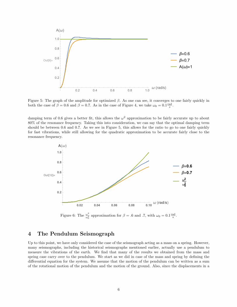
Figure 5: The graph of the amplitude for optimized β. As one can see, it converges to one fairly quickly inboth the case of β = 0.6 and β = 0.7. As in the case of Figure 4, we take ω0 = 0.1 rad

s .

damping term of 0.6 gives a better fit, this allows the ω2 approximation to be fairly accurate up to about80% of the resonance frequency. Taking this into consideration, we can say that the optimal damping termshould be between 0.6 and 0.7. As we see in Figure 5, this allows for the ratio to go to one fairly quicklyfor fast vibrations, while still allowing for the quadratic approximation to be accurate fairly close to theresonance frequency.

��������

0.02 0.04 0.06 0.08 0.10ω (rad/s)

0.2

0.4

0.6

0.8

1.0

A(ω)

β=0.6

β=0.7

ω2

ω02

Figure 6: The ω2

ω20

approximation for β = .6 and .7, with ω0 = 0.1 rads .

4 The Pendulum Seismograph

Up to this point, we have only considered the case of the seismograph acting as a mass on a spring. However,many seismographs, including the historical seismographs mentioned earlier, actually use a pendulum tomeasure the vibrations of the earth. We find that many of the results we obtained from the mass andspring case carry over to the pendulum. We start as we did in case of the mass and spring by defining thedifferential equation for the system. We assume that the motion of the pendulum can be written as a sumof the rotational motion of the pendulum and the motion of the ground. Also, since the displacements in a

6

seismograph are very small, we assume that sin θ ≈ θ. Therefore, the equation of motion is

m(Lθ + up) = −mg sin θ − bLθ = −mgθ − bLθ=⇒ mLθ + bLθ +mgθ = −mup

=⇒ θ +b

mθ +

g

Lθ = − 1

Lup, (8)

where b is the damping term, m is the mass, L is the length of the pendulum, and g is the gravitationalacceleration. We define ω2

0 = gLκ2 and β = β0

ω0= bL

mω0κ2 . Substituting these values into (8), we have

θ + βω0θ + ω20θ = − 1

Lup(t) (9)

This is the same differential equation we obtained for the mass and spring system. Therefore, we can applyall of the results we obtained from the case of the mass and spring system to the pendulum. In particular,we can say for frequencies higher than the resonance frequency of the system, the position of the pendulumis proportional to the position of the ground and that for frequencies lower than the resonance frequency, theposition of the pendulum tracks the acceleration of the ground. Since most earthquakes tend to fall withinthe 0.05 to 2 Hz range, we check what value the reduced length of the pendulum we would need for eitherof those situations.We first look at a resonance frequency of 3 Hz, which allows our seismograph to act likean accelerometer. We see that f0 = ω0

2π = 12π

√gL , so for f0 = 3 Hz, we have L = g

36π2 ≈ 30cm, assumingg = 9.81m

s2 . This is a very reasonable length, achievable by anyone with a desire to record earthquakes.Now, we look at the case of 0.1 Hz, in which would allow our seismograph to track the position of

the ground. We see that for f0 = .1 Hz, we have L = g.04π2 ≈ 25m. This is significantly larger, and it

would be very difficult to make such a pendulum that could accurate track earthquakes. How, then, does apendulum seismograph track the position of the ground? The answer comes from a way of positioning thependulum that creates a system that has an effective length much larger than the actual length or reducedlength of the pendulum. One can take a horizontal pendulum, and then tilt it at some angle α, as shownin Figure 7. This will create a system like a vertical pendulum, however, now the effective gravitationalacceleration on the pendulum is now g sinα instead of g. Now instead of the resonant frequency being

f0 = 12π

√gL , we have f0 = 1

2π

√g sinαL [4]. Suppose we want our pendulum to have a length of 30cm as

in the case of the resonance frequency of 3 Hz. The angle α we must tilt the horizontal pendulum is then

α = arcsin(

4π2Lf20

g

)= arcsin

((4)(0.3)(0.1)π2

9.81

)≈ 7◦. This would correspond to tilting the pendulum about

3.5mm above its horizontal position. However, in practice, this method has limited precision, as the frictionat the pivot points ultimately hampers how well the amplitudes can be recorded.

5 Zero Length Spring Pendulum

We have already investigated the two simplest forms for a seismograph, the mass and spring system and thependulum. The theory behind these and essentially all seismographs are the same. However, in practice, boththese forms are somewhat difficult to use when actually recording earthquakes. This is due to the difficultyof getting a sufficiently low resonance frequency. As stated earlier, when the frequency of the ground’smotion is much higher than the resonance frequency, the position of the seismograph’s mass element isproportional the position of the ground. However, getting a sufficiently small resonance frequency also assistswhen using the seismograph as an accelerometer. Let’s examine a resonance frequency f0 = 3 Hz. Then

∆XA(ω) = 1ω2

0∆(d2UAdω2

)= 1

36π2 ∆(d2UAdω2

). Therefore, in order for the seismograph to move one millimeter,

the measured acceleration would have to change by 0.36ms2 . This is a very large change in acceleration, and

is not nearly sensitive enough to be usable in scientific studies.To create oscillators with much lower natural frequencies, scientists and engineers have developed several

different devices. One such device is the zero length spring pendulum. This device hinges on what is calleda zero initial length spring. This special type of spring is one that exerts a force that is proportional to thelength it has been stretched. That is, when no force is pulling on the spring, its length can be treated aszero. One does this by making a spring that has tension even when no outside force is applied. Then, when

7

Figure 7: A diagram of how a tilted horizontal pendulum can have an effective length much larger than itsactual length [4].

the spring is being pulled by an outside force, it will not stretch until the magnitude of the force is largerthan some value. The tension in the spring is designed so that the force needed to expand it to any lengthL larger than its actual length is proportional to L, giving it the desired zero initial length [1].

We make the zero length spring pendulum by using this zero initial length spring in conjunction witha pendulum. As shown in Figure 8, we do this by taking a rod with a mass M on one end, and attachingthe other end to a wall via a hook. This forms a pivot between the rod and the wall, and the rod is free torotate about the pivot point. One end of the spring is then attached to the wall at some distance a abovethe pivot. The other end is attached to the rod at some distance b from the pivot. When the length ofthe spring has been extended to L, we can define the magnitude of the torque on the system due to thespring as τs = s× F = kLs, where s is the distance between the pivot and the point at which the spring isperpendicular to the pivot. We then note that s = a sinβ, which by the law of sines is also equal to b sin θ.So the torque on the system due to the spring is τs = kLb sin θ. To calculate the torque on the system dueto the gravitational force, we take τg = d×F = Mgd sin θ. To find the equilibrium force, we equate the twotorques to get

kLb sin θ = Mgd sin θ

=⇒ kLb = Mgd (10)

This is a relationship not based upon any angle, therefore any point could be the equilibrium position ifthese conditions are satisfied. This can be thought of as an oscillator with an infinite period, or a resonancefrequency of zero. In practice, this is not possible, since there will always be some error in the exactproportions of the values, but it is easy for a zero length spring pendulum to achieve a period of 15 to 30seconds, and periods as high as 80 seconds have been achieved in especially sensitive seismographs [1]. Inthe case of an accelerometer, this will produce a much clearer reading in the instrument for small changesin acceleration. For instance, take a period of 30 seconds, which corresponds to f0 = 0.03 Hz. Then,

∆XA(ω) = 1ω2

0∆(d2UAdω2

)≈ 1

0.01∆(d2UAdω2

). Then, a change of one millimeter in the accelerometer would

correspond to a change of 10−5 ms2 . This allows for very sensitive measurements the change of acceleration.

8

Figure 8: A drawn diagram of the zero length spring pendulum [6].

6 Conclusion

From these derivations and calculations, we can see that while the seismograph is a conceptually simpleinstrument, being based off of the humble damped oscillator, it provides a wealth of complexities that areworth exploring. We see that the damping coefficient needs especially careful consideration. It is critical forallowing the seismograph to accurately model either the position or acceleration of the ground, and could leadto difficulties if it is not calibrated accurately. The various configurations of the system also are of interest,as scientists and engineers throughout the ages have worked to derive ever more precise measurements. Thependulum measurements of the 19th century eventually led to much more complex devices like the zerolength spring pendulum. Even today, ever more complex machinery is being developed, though it is allbased off of the simple harmonic oscillator.

9

References

[1] Aki, Keiiti and Richards, Paul G., “Quantitative Seismology,” Sausalito: University Science Books,2002, 602-603.

[2] Ammon, Charles J., “Ground Motion Range.” http://eqseis.geosc.psu.edu/∼cammon/HTML/Classes/IntroQuakes/Notes/.

[3] Bolt, Bruce A., “Earthquake,” Encyclopedia Brittanica https://www.britannica.com/science/earthquake-geology.

[4] Denton, Paul, “Building A Simple Seismometer,” British Geological Survey https://www.bgs.ac.uk/downloads/start.cfm?id=659.

[5] Dewey, James and Byerly, Perry, “The Early History of Seismometry,” U.S. Geological Survey https://earthquake.usgs.gov/learn/topics/eqsci-history/early-seismometry.php.

[6] Lahr, John, “Zero Length Spring Pendulum,” http://www.jclahr.com/science/psn/zero/winding/gravity sensor.html.

[7] “Seismic Wave,” Encyclopedia Brittanica, https://www.britannica.com/science/seismic-wave.

[8] “Seismograph,” Encyclopedia Brittanica, https://www.britannica.com/science/seismograph.

[9] “Seismograph Background,” Incorporated Research Institutions for Seismology, http://www.iris.edu/hq/files/programs/education and outreach/aotm/8/Seismograph Background.pdf.

[10] “Seismographs - Keeping Track of Earthquakes,” U.S. Geological Survey https://earthquake.usgs.gov/learn/topics/keeping track.php.

10