an exploration of chaos in electrical circuits
TRANSCRIPT
Bard College Bard College
Bard Digital Commons Bard Digital Commons
Senior Projects Spring 2016 Bard Undergraduate Senior Projects
Spring 2016
An Exploration of Chaos in Electrical Circuits An Exploration of Chaos in Electrical Circuits
Ryan Ann O'Connell Bard College, [email protected]
Follow this and additional works at: https://digitalcommons.bard.edu/senproj_s2016
Part of the Electrical and Electronics Commons
This work is licensed under a Creative Commons Attribution-Noncommercial-No Derivative Works 4.0 License.
Recommended Citation Recommended Citation O'Connell, Ryan Ann, "An Exploration of Chaos in Electrical Circuits" (2016). Senior Projects Spring 2016. 326. https://digitalcommons.bard.edu/senproj_s2016/326
This Open Access work is protected by copyright and/or related rights. It has been provided to you by Bard College's Stevenson Library with permission from the rights-holder(s). You are free to use this work in any way that is permitted by the copyright and related rights. For other uses you need to obtain permission from the rights-holder(s) directly, unless additional rights are indicated by a Creative Commons license in the record and/or on the work itself. For more information, please contact [email protected].

An Exploration of Chaotic
Behavior in Electrical Circuits
Ryan O’Connell
A Senior Project presented for the degree of
Bachelor of Arts
Physics Division of Science, Mathematics, and Computing
Bard College
Annandale-on-Hudson, NY
May 2016
An Exploration of Chaotic Behavior in
Electrical Circuits
Ryan O’Connell
Abstract
This senior project investigates chaotic behavior and controlled chaos in electrical
circuits. It primarily focuses on two types of circuits: one with a varicap diode
and one with a operational amplifier based Chua diode. These are the non-linear
elements of the circuit that produce chaotic behavior in voltage outputs. Attempts
to get the circuits to function correctly were unsuccessful, but the project includes a
theoretical investigation of the chaotic behavior of the circuits through bifurcations
and period doubling, as well as ways this behavior could be theoretically controlled.
2

to Kim for being strong for me.
3

Acknowledgements
I want to thank the Physics department at Bard College for their patience,
instruction, and support throughout my time here. I would specifically like to thank
my senior project adviser Matthew Deady for his guidance, encouragement, and
motivation. I would also like to thank James Belk for providing a punch-line at the
end of every class and for strengthening my interest in chaos theory.
Lastly, I am very grateful to have such a caring and loving support system of
friends and family, both at school and home, that keep me motivated, focused, and
happy. I sincerely don’t know where I would be without all of you and your love.
4
Contents
1 Introduction 7
1.1 What is Chaos? . . . . . . . . . . . . . . . . . . . . . . . . . . . . . . 7
1.2 Attractors, Strange Attractors, and Fractals . . . . . . . . . . . . . . 9
1.3 Lorenz Attractor . . . . . . . . . . . . . . . . . . . . . . . . . . . . . 10
1.4 The Logistic Equations and Bifurcation Diagrams . . . . . . . . . . . 11
1.5 Chaos in Physical Systems . . . . . . . . . . . . . . . . . . . . . . . . 14
2 Varicap Diode Circiut 15
2.1 How It Works . . . . . . . . . . . . . . . . . . . . . . . . . . . . . . . 15
2.2 Voltage-Dependent Capacitance as a Means of Chaotic Behavior . . . 16
2.3 Reverse-Recovery Time as a Means of Chaotic Behavior . . . . . . . . 19
3 Chua’s Circuit 23
3.1 The Classical Chua’s Circuit . . . . . . . . . . . . . . . . . . . . . . . 23
3.2 The Double Scroll . . . . . . . . . . . . . . . . . . . . . . . . . . . . . 25
3.3 Variations of Chua’s Circuit . . . . . . . . . . . . . . . . . . . . . . . 27
3.4 Controlling Chaos . . . . . . . . . . . . . . . . . . . . . . . . . . . . . 32
4 Conclusion 36
A Mathematica Code 38
A.1 Lorenz Attractor . . . . . . . . . . . . . . . . . . . . . . . . . . . . . 38
A.2 Double Scroll Attractor . . . . . . . . . . . . . . . . . . . . . . . . . . 38
A.3 Matsumoto’s Double Scroll Attractor . . . . . . . . . . . . . . . . . . 39
5

An Exploration of Chaotic Behavior in Electrical Circuits
A.4 Chua Oscillator, Failed . . . . . . . . . . . . . . . . . . . . . . . . . . 39
6 Chapter 0 Ryan O’Connell

Chapter 1
Introduction
1.1 What is Chaos?
What does the word “chaos” bring to mind. The average person would probably
say it is synonymous with dysfunction, disorder, or confusion. Ask a physicist or
mathematician and you would get a much more complex answer. Chaos, in the
mathematical sense, is a type of behavior that is exhibited by particular dynamical
systems which have a sensitive dependence on initial conditions. [20] This sensitive
dependence has been referred to as the butterfly effect. [13] This is the idea that a
butterfly in China can flap its wings and through a series of events that happened
because of that flap, Texas experiences a hurricane. Basically, it is a dramatized
expression of a simple notion: small changes produce large-scale results in intercon-
necting and complex environments.
To better understand this, let’s look at the simple example of the rounded edge
pool table:
Figure 1.1: rounded-edge pool table
For this example, let’s neglect friction so that the pool ball will continue its
7
An Exploration of Chaotic Behavior in Electrical Circuits
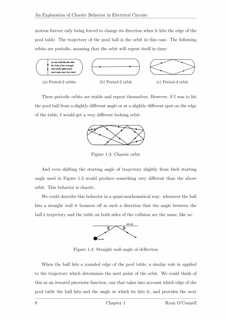
motion forever only being forced to change its direction when it hits the edge of the
pool table. The trajectory of the pool ball is the orbit in this case. The following
orbits are periodic, meaning that the orbit will repeat itself in time:
(a) Period-2 orbits (b) Period-2 orbit (c) Period-4 orbit
These periodic orbits are stable and repeat themselves. However, if I was to hit
the pool ball from a slightly different angle or at a slightly different spot on the edge
of the table, I would get a very different looking orbit:
Figure 1.3: Chaotic orbit
And even shifting the starting angle of trajectory slightly from theh starting
angle used in Figure 1.3 would produce something very different than the above
orbit. This behavior is chaotic.
We could describe this behavior in a quasi-mathematical way: whenever the ball
hits a straight wall it bounces off in such a direction that the angle between the
ball’s trajectory and the table on both sides of the collision are the same, like so:
Figure 1.4: Straight wall angle of deflection
When the ball hits a rounded edge of the pool table, a similar rule in applied
to the trajectory which determines the next point of the orbit. We could think of
this as an iterated piecewise function, one that takes into account which edge of the
pool table the ball hits and the angle at which its hits it, and provides the next
8 Chapter 1 Ryan O’Connell

An Exploration of Chaotic Behavior in Electrical Circuits
part of the orbit. We could then continuously take the output of our hypothetical
piecewise function and put it back into our hypothetical piecewise function to get
the next point of our orbit, and continue to do this forever. This iterated function
would produce chaotic behavior. Not all iterated functions do. Some, like f(x) =
2x, just produce a series where each element is twice the value of the one before
it. But in special cases, all of which have some nonlinear element to them, like the
rounded edge pool table, the iterated function can produce chaos — deterministic,
but unpredictable (because of initial condition sensitivity).
1.2 Attractors, Strange Attractors, and Fractals
This next, very famous, example may come as a surprise to someone who has
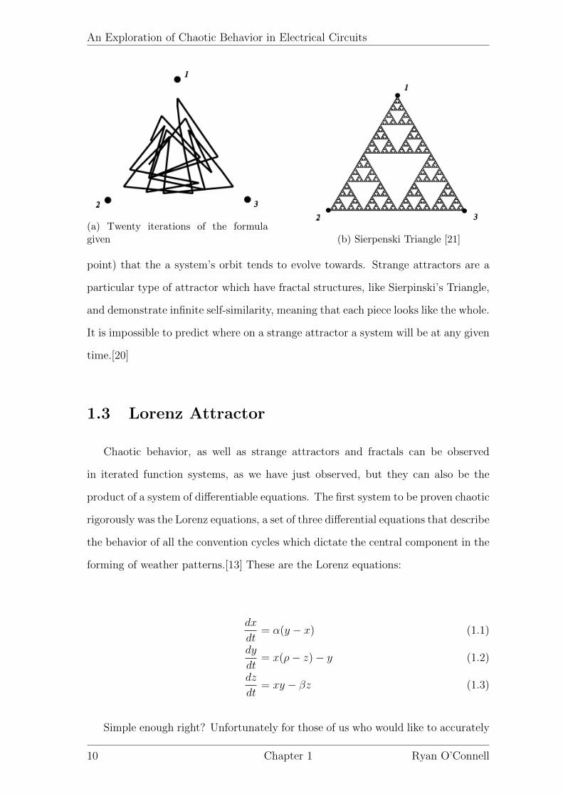
never seen it. Let’s consider the following iterated formula: We have three points
equidistant and the same angle apart from each other:
Figure 1.5: Vertex points of equilateral triangle
We choose any point within the triangle these three points connect to make to
be our starting point. At random, we will choose an integer from 1 to 3 and draw
a line from our starting point, halfway to the corresponding point. From there, we
iterate through this formula some large number of times. This process will create
something that looks disorderly or chaotic like Figure 1.6a.
If we repeat this process, but for an extremely high number of iterations (some-
thing like 100,000) and only plotted the endpoints of our lines, we would get a
completely different image resembling that of Figure 1.6b.
This image is known as Sierpinski’s Triangle and it is one of the simplest fractals.
Fractals are attractors of chaotic systems. Attractors are groups of points (or a single
Chapter 1 Ryan O’Connell 9
An Exploration of Chaotic Behavior in Electrical Circuits
(a) Twenty iterations of the formulagiven (b) Sierpenski Triangle [21]
point) that the a system’s orbit tends to evolve towards. Strange attractors are a
particular type of attractor which have fractal structures, like Sierpinski’s Triangle,
and demonstrate infinite self-similarity, meaning that each piece looks like the whole.
It is impossible to predict where on a strange attractor a system will be at any given
time.[20]
1.3 Lorenz Attractor
Chaotic behavior, as well as strange attractors and fractals can be observed
in iterated function systems, as we have just observed, but they can also be the
product of a system of differentiable equations. The first system to be proven chaotic
rigorously was the Lorenz equations, a set of three differential equations that describe
the behavior of all the convention cycles which dictate the central component in the
forming of weather patterns.[13] These are the Lorenz equations:
dx
dt= α(y − x) (1.1)
dy
dt= x(ρ− z)− y (1.2)
dz
dt= xy − βz (1.3)
Simple enough right? Unfortunately for those of us who would like to accurately
10 Chapter 1 Ryan O’Connell

An Exploration of Chaotic Behavior in Electrical Circuits
know the weather next Saturday, this system of equations exhibits chaotic behavior.
An orbit of this system mapped out over time while plotting x, y, and z against each
other will look like this:
Figure 1.7: The Lorenz Attractor
This is Lorenz Attractor. [23] It is a strange attractor and it is self-similar and
is sensitive to initial conditions. The orbit is completely deterministic, however, it
is impossible to predict which part of the attractor the orbit will be on at any given
time. If you started simultaneous orbits of this system with initial conditions one-
millionth of a decimal place different from each other, their orbits would start off
identical, but eventually would show slight differences that would ultimately result
in completely different orbits. This is a main reason why weather predictions are
very difficult to make with any degree of accuracy past a few days.
1.4 The Logistic Equations and Bifurcation Dia-
grams
As previously shown, chaos is not easily defined and has many components to
identifying and explaining it. All of the examples I have just presented evolve over
time, but time doesn’t have to be the parameter that is evolving in the system for
Chapter 1 Ryan O’Connell 11
An Exploration of Chaotic Behavior in Electrical Circuits
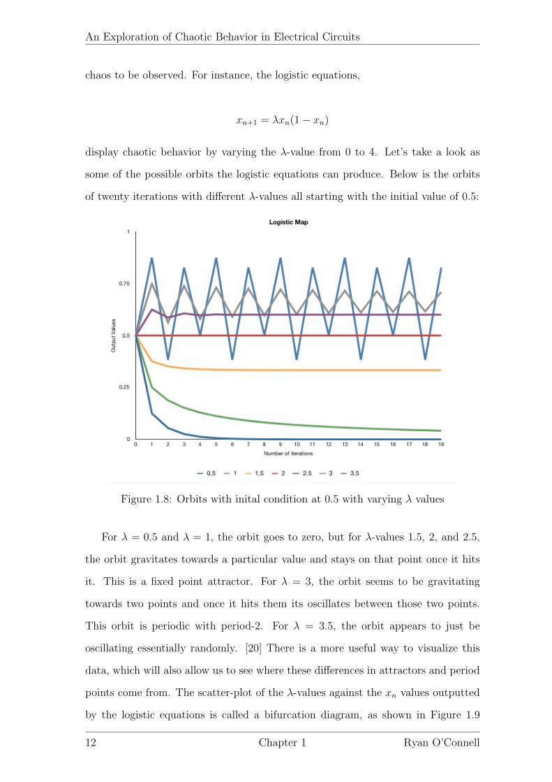
chaos to be observed. For instance, the logistic equations,
xn+1 = λxn(1− xn)
display chaotic behavior by varying the λ-value from 0 to 4. Let’s take a look as
some of the possible orbits the logistic equations can produce. Below is the orbits
of twenty iterations with different λ-values all starting with the initial value of 0.5:
Figure 1.8: Orbits with inital condition at 0.5 with varying λ values
For λ = 0.5 and λ = 1, the orbit goes to zero, but for λ-values 1.5, 2, and 2.5,
the orbit gravitates towards a particular value and stays on that point once it hits
it. This is a fixed point attractor. For λ = 3, the orbit seems to be gravitating
towards two points and once it hits them its oscillates between those two points.
This orbit is periodic with period-2. For λ = 3.5, the orbit appears to just be
oscillating essentially randomly. [20] There is a more useful way to visualize this
data, which will also allow us to see where these differences in attractors and period
points come from. The scatter-plot of the λ-values against the xn values outputted
by the logistic equations is called a bifurcation diagram, as shown in Figure 1.9
12 Chapter 1 Ryan O’Connell
An Exploration of Chaotic Behavior in Electrical Circuits
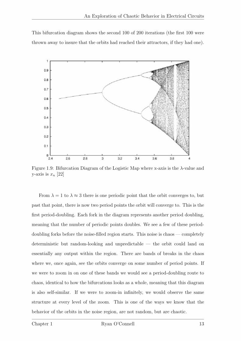
This bifurcation diagram shows the second 100 of 200 iterations (the first 100 were
thrown away to insure that the orbits had reached their attractors, if they had one).
Figure 1.9: Bifurcation Diagram of the Logistic Map where x-axis is the λ-value andy-axis is xn [22]
From λ = 1 to λ ≈ 3 there is one periodic point that the orbit converges to, but
past that point, there is now two period points the orbit will converge to. This is the
first period-doubling. Each fork in the diagram represents another period doubling,
meaning that the number of periodic points doubles. We see a few of these period-
doubling forks before the noise-filled region starts. This noise is chaos — completely
deterministic but random-looking and unpredictable — the orbit could land on
essentially any output within the region. There are bands of breaks in the chaos
where we, once again, see the orbits converge on some number of period points. If
we were to zoom in on one of these bands we would see a period-doubling route to
chaos, identical to how the bifurcations looks as a whole, meaning that this diagram
is also self-similar. If we were to zoom-in infinitely, we would observe the same
structure at every level of the zoom. This is one of the ways we know that the
behavior of the orbits in the noise region, are not random, but are chaotic.
Chapter 1 Ryan O’Connell 13

An Exploration of Chaotic Behavior in Electrical Circuits
1.5 Chaos in Physical Systems
As we have already observed to a certain extent, chaos can be observed in many
physical systems. The logistic map has been used to model the stability of ecosys-
tems. A system as simple as a double pendulum or a 3-body system are chaotic
systems. While the individual parts of the systems are simple and easy to predict,
when these parts interact with other simple parts, the sensitivity on initial con-
ditions is amplified and the system becomes chaotic. For instance, if you took a
break shot in pool, the balls will hit into each other in such a way that, even if
you tried your hardest to hit them in the exact same way, you would never be able
to replicate. Think of it like a 15-body problem — extremely dependent on initial
conditions. Perhaps not as obviously as these physical systems have, particular elec-
trical circuits also exhibit chaotic behavior. This project is an investigation into the
different ways we can observe this behavior in two of these particular circuits. The
two circuits I have chosen to focus my exploration on are the varicap diode circuit
and the Chua circuit. the diodes in both cases provide the non-linearity needed to
exhibit chaotic behavior. The varicap diode circuit is much simpler in its structure
as it is essentially just a RLD circuit (that at times acts like an RLC circuit, but
that will be explained later). The Chua circuit is a bit more complicated with an
operational amplifier based diode and a few more reactive elements. Equipped with
the chaos theory vocabulary to describe the behavior of these chaotic circuits, let’s
take a looks at the varicap diode circuit.
14 Chapter 1 Ryan O’Connell

Chapter 2
Varicap Diode Circiut
2.1 How It Works
First, let’s look at the behavior of the varicap diode circuit. The diode’s name
comes from the combination of the words “variable” and “capacitance” because
its capacitance is voltage-dependent. There were three major papers published
describing the behavior of this diode during 1981 and 1982, which I have drawn
most of my understanding of the circuit from. The circuit containing the varicap
diode that exhibits period doubling and chaotic behavior looks like this: where
Figure 2.1: Varicap Diode Circuit
the circled element is the varicap diode and the elements labeled (b) and (c) are
in reference to its behavior under specific conditions. The varicap diode exploits
the voltage-variable property of the junction capacitance, which every diode has to
some extent but in most cases tries to minimize. In the varicap diode, the depletion
15

An Exploration of Chaotic Behavior in Electrical Circuits
region between the P and N parts of the diode is large, making the diode essentially
a capacitor in reverse bias. This is where (b) can be switched in for the varicap diode
in the above circuit. In forward bias, the diode conducts and could be thought to
be replaced by an emf with voltage VF . This is where (a) can be switched in for
the varicap diode in the above circuit. However, the diode will not conduct until Vf
is reached and will stay at Vf for the remaining time the circuit is in forward bias.
Until then, the diode does not conduct but instead has a fixed capacitance. When
the current through the diode passes through zero, the diode does not immediately
stop conducting. It takes some reverse-recovery time to stop conducting completely.
2.2 Voltage-Dependent Capacitance as a Means
of Chaotic Behavior
There are two ways to exhibit the chaotic behavior of the circuit above. The
first of which was first discovered by Paul S. Linsay in 1981 [1] and later expanded
upon by James Testa, Jose Perez and Carson Jeffries the following year [3]. Linsay’s
experimentation was done in response to Feigenbaum’s theory of non-linear systems
that exhibit period doubling, which states that their behavior, and specifically their
bifurcation and period doubling patterns, follow universal laws independent of the
equations that describe their particular behavior. The goal of Linsay’s experiment
was to show that this theory holds for physical systems, and in particular, for a
driven anharmonic oscillator. Feigenbaum’s theory states that given some system
described by
dxidt
= Fi(x1, x2, ..., xN)
for i = 1, 2, ..., N and given that xi(t) are periodic with period Tn = 2nT0 at λ = λn,
the recurrence relation,
λn+1 − λnλn+2 − λn+1
= δ
16 Chapter 2 Ryan O’Connell

An Exploration of Chaotic Behavior in Electrical Circuits
is satisfied, where δ is the Feigenbaum convergence rate, which, for quadratic ex-
trema, is 4.669. For an electrical circuit like this one, the xi(t) is the current flowing
through the system and the λ is the amplitude of the drive voltage at a particular
subharmonic, n. Linsay chose to observe this circuit’s chaotic behavior by analyz-
ing its spectral peaks at different drive voltages, which would be directly influenced
by the diode’s capacitance dependence on said drive voltages. This dependence is
described by this equation:
C(V ) =C0
(1 + Vφγ
)
where C0 = 81.8ρF, γ = 0.44, and φ = 0.6V determined by measured values of
capacity. A spectrum analyzer was connected to the circuit between the inductor
and the resistor, see Figure 2.2, to measure the subharmonics at specific frequencies
Figure 2.2: Varicap Diode Circuit with Spectrum Analyzer
which would occur as the drive voltage was increased. At very low drive voltages, the
circuit acted like a regular RLC circuit in series, where the resonance frequency was
found to be 1.78MHz. As the drive voltages increased, spectral peaks were observed,
the first being at the frequency one-half of the resonance frequency. Three more
subharmonic frequencies were observed as the drive voltage increased: at one-fourth,
one-eighth, and one-sixteenth the resonance frequency. The calculated value of δ, the
Chapter 2 Ryan O’Connell 17

An Exploration of Chaotic Behavior in Electrical Circuits
convergence rate in Linsay’s experiment, for which he was able to compute two given
the data collected, is displayed in Figure 2.3. The Feigenbaum convergence rate for
quadratic extremum is very close to the calculated values of δ in this experiment,
therefore giving experimental evidence of a physical system exhibiting Feigenbaum’s
theory of nonlinear systems that exhibit period doubling.
Figure 2.3: Table used to compare the difference in Vthreshold for each subharmonicto calculate the convergence rate
The period-doubling of spectral peaks is displayed in this spectrum, where the
numbers at the top of the peaks corresponds to the order of appearance and the
y-axis is the amplitude in decibels:
Figure 2.4: Period-Doubling Spectral Peaks [1]
When translated into a bifurcation diagram, this spectral peaks appear in the
following fashion as shown in Figure 2.5a. (It is important to note that this does
not look like a traditional bifurcation diagram since the peaks remain as new peaks
appear)
Increasing the drive voltage past this point, produced chaotic behavior as exhib-
ited in Figure 2.5b. Replacement of the varicap diode with a capacitor in parallel
18 Chapter 2 Ryan O’Connell

An Exploration of Chaotic Behavior in Electrical Circuits
(a) Bifurcation Diagram of SpectralPeaks of Varicap Diode Circuit (b) The full onset of chaos [1]
with a 1N4154 diode which had the same resonant frequency as the varicap diode
set up did but lacked the period-doubling behavior, proves, according to Linsay,
that the chaotic nature of the circuit is due to the nonlinear capacity of the varicap
diode as described by these three equations:
Vc =Q
CVc= (1 +
Vcφ
)γQ
C0
LdI
dt= V0 sin (2πf1t)Vc −RI
dQ
dt= I
whose solutions, according to Linsay, support the data.
2.3 Reverse-Recovery Time as a Means of Chaotic
Behavior
As I had mentioned previously, there is a secondary path to proving the vari-
cap circuit presented exhibits chaotic behavior. Instead of observing the voltage-
dependent capacitance, one could prove that the large reverse-recovery time of the
Chapter 2 Ryan O’Connell 19
An Exploration of Chaotic Behavior in Electrical Circuits
varicap diode is the property of this diode that produces the chaotic behavior.
Rollins and Hunt actually speculated that the large reverse-recovery time is, in
fact, the only reason for the chaotic behavior, [2] not the voltage-dependent capaci-
tance that Linsay had suspected, but never actually proved, to be the reason for the
period-doubling. Rollins and Hunt give a step by step procedure on how to observe
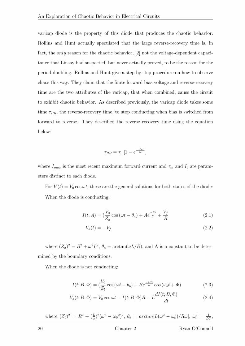
chaos this way. They claim that the finite forward bias voltage and reverse-recovery
time are the two attributes of the varicap, that when combined, cause the circuit
to exhibit chaotic behavior. As described previously, the varicap diode takes some
time τRR, the reverse-recovery time, to stop conducting when bias is switched from
forward to reverse. They described the reverse recovery time using the equation
below:
τRR = τm[1− e−|Im|Ic ]
where Imax is the most recent maximum forward current and τm and Ic are param-
eters distinct to each diode.
For V (t) = V0 cosωt, these are the general solutions for both states of the diode:
When the diode is conducting:
I(t;A) = (V0Za
cos (ωt− θa) + Ae−RtL +
VfR
(2.1)
Vd(t) = −Vf (2.2)
where (Za)2 = R2 + ω2L2, θa = arctan(ωL/R), and A is a constant to be deter-
mined by the boundary conditions.
When the diode is not conducting:
I(t;B,Φ) = (V0Zb
cos (ωt− θb) +Be−2RtL cos (ωbt+ Φ) (2.3)
Vd(t;B,Φ) = V0 cosωt− I(t;B,Φ)R− LdI(t;B,Φ)
dt(2.4)
where (Zb)2 = R2 + (L
ω)2(ω2 − ω0
2)2, θb = arctan[L(ω2 − ω20)/Rω], ω2
0 = 1LC
,
20 Chapter 2 Ryan O’Connell

An Exploration of Chaotic Behavior in Electrical Circuits
ω2b = ω2
0 − ( R2L
)2, and B and Φ are constants to be determined by the boundary
conditions.
Given an alternating current, the diode will go through different cycles of specific
behavior. An example of three of these cycles that Rollins and Hunt found using
the system modeled above, is given in Figure 2.6.
Figure 2.6: Three cycles of the varicap circuit. The top graph depicts the currentacross the diode as a function of time, and the bottom graph depicts the voltageacross the diode also as a function of time. ti(n)’s refer to key times when somethingabout the diode’s behavior has changed. [2]
In this diagram, t1(n) depicts the beginning of the time that the diode will be
conducting, so the diode will be in forward bias, and the start of the n-th cycle.
t2(n) is the time at which the current passes through zero. Notice that the diode is
still conducting, making this the start of τRR. The reverse-recovery time is dictated
in this case by Im, which is the lowest or highest point of I during the cycle being
considered. One would assume, correctly, then that t3(n) = t2(n) + τRR(n).
Now for the interesting part. The value of t3(n) is determined on a 2-case basis.
Case 1: If current at t3(n) is passing through the diode in the reverse direction, then
Chapter 2 Ryan O’Connell 21
An Exploration of Chaotic Behavior in Electrical Circuits
the diode will stop conducting and it is not until the voltage across the diode is back
at -Vf , that the next cycle begins, as depicted in Figure 2.6. Case 2: If current at
t3(n) is passing through the diode in the forward direction, then the diode does not
stop conducting and the next cycle starts with t1(n+ 1) = t3(n). This is where the
nonlinearity of the circuit that is needed to produce the chaotic behavior comes from.
Since the previously stated system of equations 2.1-2.4 fully describe the behavior
of the system, each new |Imax|n can be determined from the previous cycle’s one,
given a set of initial conditions, the trajectory of the voltage across the diode is
deterministic, but slight changes in the initial conditions will greatly influence the
outcome once a different case of t3(n) is satisfied. This is sensitive dependence on
initial conditions stemming from a nonlinear element of the system, which is our
principle definition of chaos. This is how Rollins and Hunt identified the central
component in the production of chaotic behavior in the varicap diode circuit.
In a later paper by Mariz de Mores and Anlage a more detailed depiction of how
the p-n junction in the diode effects the nonlinearities that the reverse-recovery time
depends on through the different stages of the circuit. [17] They, unlike Rollins and
Hunt, do not make the assertion of the reverse-time constant being the principle cre-
ator of chaotic behavior, but rather, chose to not make a distinction between effects
of the nonlinear capacitance and reverse-recovery time of the diode, as they can be
similar, as they both take the history of the circuit into account when determining
the trajectory of the system.
This concludes my discussion of the varicap diode circuit. Now that we are
familiar with the way in which chaotic behavior can be seen in circuit systems, let’s
take a look at the, slightly more complex, Chua Circuit and the many ways it (and
its variations) exhibits chaotic behavior.
22 Chapter 2 Ryan O’Connell
Chapter 3
Chua’s Circuit
3.1 The Classical Chua’s Circuit
The second simple circuit exhibiting chaotic behavior that I have explored is
called Chua’s circuit. One of the aspects of Chua’s circuit that makes it so attractive
to work with is that it does not require the purchase of a special element as its
nonlinear component, but instead can be made using simple inductors, resistors,
capacitors, and a couple of operational amplifiers as shown in Figure 3.1a with
the right-most section of the circuit being referred to as Chua’s diode, a nonlinear
resistor. The original Chua circuit only has one inductor, but I attempted to use
two in series to get the correct inductance, as I did not have an inductor of the value
needed. Inductors in series add their values, so this should not have effected the
circuit at all. The equations that govern this circuit are as follows, all of which can
be easily obtained with the exception of id(v1) which is a bit more complicated as
it is the current through the diode as a function of the voltage across C1:
C1dv1dt
=v2 − v1R
− id(v1)
C2dv2dt
=(v1 − v2)
R− il
LdiLdt
= −v2
23

An Exploration of Chaotic Behavior in Electrical Circuits
Value Component Schematic Label
10nF Capacitor C1
100nF Capacitor C2
10mH Inductor L1
10mH Inductor L2
1.5kΩ Potentiometer R220Ω Resistor R1
220Ω Resistor R2
2.2kΩ Resistor R3
22kΩ Resistor R4
22kΩ Resistor R5
3.3kΩ Resistor R6
Table 3.1: Element Values for the Chua Circuit
Here, v1 and v2 refer to the voltage across the corresponding capacitor and iL is
the current across the inductor. The m variables in id(v1) correspond to the slopes
of the line created by the relationship between the voltage across the first capacitor
and the current through the diode as Figure 3.1b displays. This piecewise function,
id(v1) is what makes this circuit non-linear and is responsible for its chaotic behavior.
(a) Chua’s CircuitSchematic
(b) The current across the Chua diode as afunction of the voltage across C1
With the guidance of [19], I attempted to construct this current with the ele-
ment values described in Table 3.1. I encountered various set-backs along the way
including a power board that was exhibiting 6V of noise. Ultimately, while trying
to measure the resonant frequency of the diode-excluded circuit, my adviser and I
determined that the values of some of the elements I was using were incorrect. Un-
24 Chapter 3 Ryan O’Connell

An Exploration of Chaotic Behavior in Electrical Circuits
fortunately, my error was caught too late in the allotted project time to reconcile,
so I will be giving a theoretical analysis of the chaotic behavior of the Chua Circuit
using some Mathematica modeling and research I have done of previously published
projects.
Modeling of the circuit equations with the help of [21], gave the following results:
Figure 3.2: Chua Circuit’s Equations plotted in the (v1(t), v2(t), iL(t)) plane as tgoes from 0 to 100
This is known as the Double Scroll strange attractor. The above orbit along the
Double Scroll attractor does not systematically move from one scroll to the other in
any kind of predicable fashion, but rather one that is unpredictable and seemingly
random, but deterministic. Other initial conditions would give a completely different
orbit, but one that still has the general shape. Adjusting parameters, such as the
inductance and the resistance of R will give you different sections of the double scroll
and periods before that of the chaotic attractor, respectively.
3.2 The Double Scroll
One of the first to publish on the appearance of the Double Scroll attractor in an
electrical circuit was T. Matsumoto, who observed the behavior of a slightly different
circuit than the one outlined above. [4] Leon O. Chua was actually the one to
discover this attractor, but had to be rushed to the hospital for an emergency surgery
Chapter 3 Ryan O’Connell 25

An Exploration of Chaotic Behavior in Electrical Circuits
after his discovery and left this work to Matsumoto to be published. This circuit
had the inductor (or inductors, in my case) switched with the second capacitor, like
so:
Figure 3.3: Matsumoto’s Chua Circuit
The equations that govern this circuit are as follows:
C1dv1dt
= R(v2 − v1)− id(v1) (3.1)
C2dv2dt
= R(v1 − v2) + il (3.2)
LdiLdt
= −v2 (3.3)
The difference in structure does lend itself to a slightly different looking attractor
for this circuit as compared to the common construction of the Chua circuit, dis-
played at the beginning of the chapter, which I will present later. Both attractors
are types of Double Scroll attractors. The attractor made by Matsumoto’s circuit
is modeled in Figures 3.4a - 3.4d.
This attractor was proven to be different from the other strange attractors known
at the time (Lorenz Attractor and Rossler’s Attractor) by comparing the signs of
the the eigenvalues on the origin to those not on the origin in each case. [4] And so,
this was the first of its own class of strange attractors, later coined by Chua as the
Double Scroll family of attractors. [5]
26 Chapter 3 Ryan O’Connell

An Exploration of Chaotic Behavior in Electrical Circuits
(a) 3-D view of Matsumoto’s Chua Cir-cuit Attractor observed after a timelapse of 300 seconds
(b) Left view of attractor where x-axis isthe voltage drop across the first capaci-tor and y-axis is the current across theinductor.
(c) Right view of attractor where x-axisis the voltage drop across the second ca-pacitor and y-axis is the current acrossthe inductor.
(d) Right view of attractor where x-axisis the voltage drop across the first capac-itor and y-axis is the voltage drop acrossthe second capacitor.
3.3 Variations of Chua’s Circuit
A slightly more canonical version of Chua’s Circuit is the Chua Oscillator. [11]
This circuit is more canonical in the sense that it exhibits a wider range of chaotic
phenomena than the classical Chua Circuit, particularly in the routes it takes to
display this chaos, as we will investigate.
Figure 3.5: Chua Oscillator Schematic Circuit as described by [12]
Chapter 3 Ryan O’Connell 27
An Exploration of Chaotic Behavior in Electrical Circuits
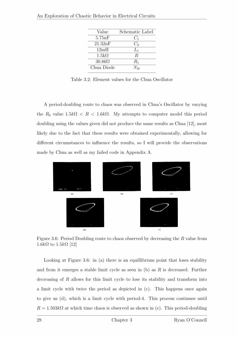
Value Schematic Label5.75nF C1
21.32nF C2
12mH L1
1.5kΩ R30.86Ω R1
Chua Diode NR
Table 3.2: Element values for the Chua Oscillator
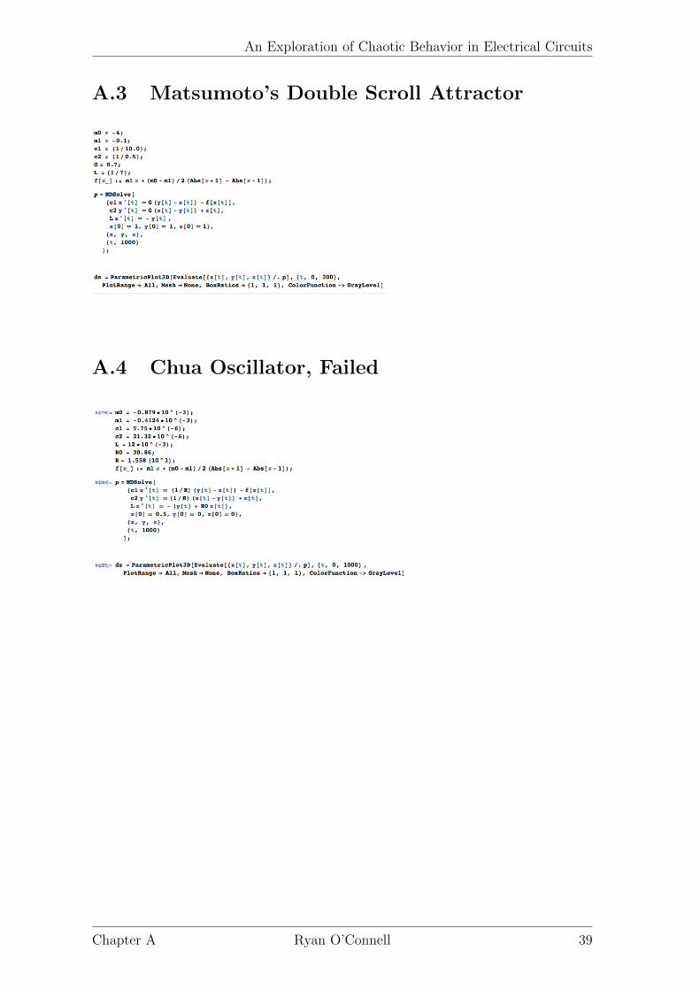
A period-doubling route to chaos was observed in Chua’s Oscillator by varying
the R0 value 1.5kΩ < R < 1.6kΩ. My attempts to computer model this period
doubling using the values given did not produce the same results as Chua [12], most
likely due to the fact that these results were obtained experimentally, allowing for
different circumstances to influence the results, so I will provide the observations
made by Chua as well as my failed code in Appendix A.
Figure 3.6: Period Doubling route to chaos observed by decreasing the R value from1.6kΩ to 1.5kΩ [12]
Looking at Figure 3.6: in (a) there is an equillibrium point that loses stability
and from it emerges a stable limit cycle as seen in (b) as R is decreased. Further
decreasing of R allows for this limit cycle to lose its stability and transform into
a limit cycle with twice the period as depicted in (c). This happens once again
to give us (d), which is a limit cycle with period-4. This process continues until
R = 1.503kΩ at which time chaos is observed as shown in (e). This period-doubling
28 Chapter 3 Ryan O’Connell

An Exploration of Chaotic Behavior in Electrical Circuits
route to chaos is just one of the routes presented by Chua, that the Chua Oscillator
can take to chaos.
Also described in [12] is the type-1 intermittency route to chaos. This route
to chaos is observed in systems that appear to be periodic in their trajectory but
experience chaotic bursts. This route to chaos was observed for R = 1.501kΩ in
the Chua Oscillator, where a stable period-3 limit cycle was observed, as shown in
Figure 3.7.
Figure 3.7: Type-1 intermittency route to chaos observed by increasing the R valuefrom 1.501kΩ to 1.502kΩ [12]
Here we see phase portraits of a stable period-3 limit cycle in the left (a) and an
intermittency near the period-3 cycle. The (b)’s are both time waveforms of v1 that
show a period-3 limit cycle and intermittent chaos near that period-3 limit cycle,
from left to right.
Chua goes on to explain that the period-doubling into chaos is not just observed
at these values of R, but that there are windows of chaos that revert back to being
periodic, and then revert back to chaos, similarly to the way the logisitc map does.
This is the another way he proves this circuit to be chaotic.
Lastly, the Chua Oscillator’s torus breakdown route to chaos is explained, this
time, by varying the values of C1 and fixing R. For specified element values and a
specified C1, a double-torus attractor with a trajectory jumping from one torus to
Chapter 3 Ryan O’Connell 29
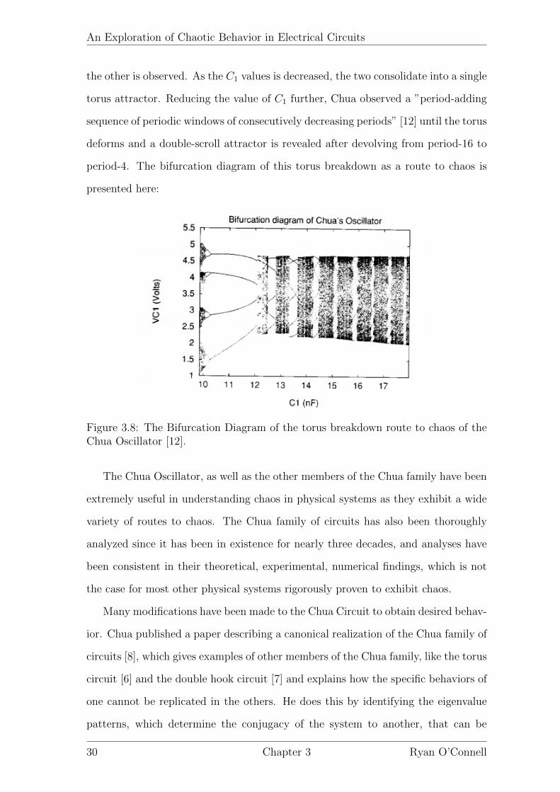
An Exploration of Chaotic Behavior in Electrical Circuits
the other is observed. As the C1 values is decreased, the two consolidate into a single
torus attractor. Reducing the value of C1 further, Chua observed a ”period-adding
sequence of periodic windows of consecutively decreasing periods” [12] until the torus
deforms and a double-scroll attractor is revealed after devolving from period-16 to
period-4. The bifurcation diagram of this torus breakdown as a route to chaos is
presented here:
Figure 3.8: The Bifurcation Diagram of the torus breakdown route to chaos of theChua Oscillator [12].
The Chua Oscillator, as well as the other members of the Chua family have been
extremely useful in understanding chaos in physical systems as they exhibit a wide
variety of routes to chaos. The Chua family of circuits has also been thoroughly
analyzed since it has been in existence for nearly three decades, and analyses have
been consistent in their theoretical, experimental, numerical findings, which is not
the case for most other physical systems rigorously proven to exhibit chaos.
Many modifications have been made to the Chua Circuit to obtain desired behav-
ior. Chua published a paper describing a canonical realization of the Chua family of
circuits [8], which gives examples of other members of the Chua family, like the torus
circuit [6] and the double hook circuit [7] and explains how the specific behaviors of
one cannot be replicated in the others. He does this by identifying the eigenvalue
patterns, which determine the conjugacy of the system to another, that can be
30 Chapter 3 Ryan O’Connell

An Exploration of Chaotic Behavior in Electrical Circuits
produced by Chua’s circuit and then states reasons for which particular eigenvalue
patterns can not be replicated by the other members of the Chua family. Ultimately,
he describes a circuit of his own creation that is general enough to, given the proper
element values and choosing the right parameters, display all of the behaviors of the
circuits in the Chua family. This canonical circuit is pictured here:
Figure 3.9: The Canonical Chua Circuit. (a) The schematic of the circuit (b) thecurrent across the non-linear resistor as a function of voltage across C1 (referred toas the v-i characteristic) [8].
where the G variables are like our m variables from previous cases. As one
can see, the are only six elements in the circuit, and only one of them is nonlinear
making for an exceedingly simple circuit for such a plethora of chaotic behavior to
be observed from. Chua goes on to prove that this circuit can realize any eigenvalue
pattern in the class of three-region symmetric, with respect to the origin, piecewise-
linear continuous vector fields which has come to define a circuit as belonging to the
Chua family. [8]
Chapter 3 Ryan O’Connell 31

An Exploration of Chaotic Behavior in Electrical Circuits
3.4 Controlling Chaos
Chaotic systems naturally exhibit a variety of different behaviors in a single orbit.
Being able to control when these naturally occurring behaviors are exhibited is very
desirable since only small changes can produce large effects, increasing efficiency.
However, it is also for these reasons, that it controlling chaos would be a difficult
task. It is also sometimes undesirable to have a system be chaotic when, for whatever
reason, you do not want sensitive dependence on initial conditions. This has been
the motivation behind recent work on controlling chaos in systems like the Chua
Circuit.
This is the line of thinking that argues for the control of chaotic systems: Ana-
lyzing a system by its performance, let’s call that P , we would see that P depends
on the time average of the function of the system state, f(x). This function of the
system state would be a function of the time dependent orbit of the system, x. For
chaotic systems, x would be the chaotic orbit on the attractor. These attractors
have periodic points on them, some stable, some unstable. Each of the unstable
period points on the attractor has its own time dependent orbit, xi and therefore
will have its own performance Pi. Since P is the weighted average of all the Pi’s,
there must exist Pi’s that are higher than P (and some that are lower).
Theoretically, giving a system initial conditions that will project its motion di-
rectly on an unstable periodic point with a large Pi would do the trick. However,
this becomes virtually impossible when dealing with chaotic systems because of their
sensitive dependence on initial conditions. It is also important to note that if you
land only near an unstable periodic point and not on it, the system’s orbit could
be repelled by the unstable periodic point. This means that you must kick the
system back towards the unstable period point. This can be done using a few dif-
ferent techniques including placing the orbit near the stable manifold of the desired
unstable periodic point, using a continuous time-delay feedback system, and the
pole-placement technique. [18]
All techniques of controlling chaos can be broken down into two categories: feed-
32 Chapter 3 Ryan O’Connell

An Exploration of Chaotic Behavior in Electrical Circuits
back and non-feedback, feedback techniques being the more versatile and widely
used method. Non-feedback control techniques require small period parametric per-
turbations which continuously kick the system back to the desired fixed point. This
is a quicker fix for chaotic behavior, but without the use of feedback, this becomes
difficult to globalize. There has been successful non-feedback control techniques
performed on the Chua Circuit, and other circuits exhibiting chaotic behavior. [10]
[9] [15] However, since the methods of feedback control methods appear to be more
common and non-feedback methods seem to be better when high-speed control is
needed (not the case here), I will focus primarily on describing and explaining some
of the ways feedback control methods have been use to control the chaotic behavior
of the Chua Circuit. The first method we will explore is a type of linear feedback
control method used on the Chua Circuit by Hwang, Hsieh and Lin. [14] The paper
cited proposed the control method of adding a voltage source in series with the in-
ductor in Chua’s circuit. Our new controlled Chua Circuit will behave according to
the following system of equations:
C1dv1dt
=v2 − v1R
− id(v1) (3.4)
C2dv2dt
=(v1 − v2)
R− il (3.5)
LdiLdt
= −v2 + u (3.6)
Our control addition, u has two parts: the first, mimics the second equation and
in doing so extends the equilibrium points of the system, and the second, cancels
out the non-control part of the equation and adds in what has the same form as a
restoring force, damping the behavior of the system around an equilibrium point.
The following is the, as previously described, equation of u:
u = k(x− y + z) + βy + kp(xref − x)
where xref is your desired reference x-coordinate.
Chapter 3 Ryan O’Connell 33

An Exploration of Chaotic Behavior in Electrical Circuits
Hwang, Hsieh and Lin observed the control of Chua’s Circuit’s chaotic behavior
from Figure 3.10a. The restoring nature of the control addition is apparent in Figure
3.10a (b) as the orbit takes an oscillatory path to the desired fixed point.
(a) [a] and [b] both depict the controllingof chaos to a fixed point, just to differentxref points [14].
(b) [a] Uses the time responses of thecontrolled system to depict the control-ling of chaos to a limit cycle of period-2and [b] illustrates u as a function of time.[14].
After establishing a control method for bringing a chaotic circuit to a desired
fixed point, Hwang, Hsieh and Lin tested their method on bringing the Chua Circuit
to a desired limit cycle. This was also successful according to Figure 3.10b
The method of feedback control not only works for fixed points and limit cycles
alike, but it also has a very small overshoot, meaning it does not usually oscillate
very much before settling on a point or cycle, making for a more efficient method of
control.
In a later paper by Tzuyin Wu and Min-Sin Chen, using a backstepper control
34 Chapter 3 Ryan O’Connell

An Exploration of Chaotic Behavior in Electrical Circuits
design, a nonlinear feedback control method for Chua’s circuit is presented which
is proven to be a ”global” control, meaning that any initial values of the system
will allow you to control the output to any periodic point. They make the case that
since chaotic systems are nonlinear, it is necessary to use a nonlinear feedback system
to globalize the control. The controlled system set up is in the same in terms of
equations 3.4-3.6, but a smooth approximation is used to describe the current across
the diode as a function of the voltage across the first capacitor that is a follows:
f(x) =2x3 − x
7
.
The function of u for this control method is much more complicated than the
previous one and is depicted in Figure 3.11.
Figure 3.11: The control non-linear function, u. [16]
Wu and Chen go on to rigorously prove the stability and globalization of this
equation of u.
All of the articles I was able to find on controlling chaos were theoretical and
numerical, but not experimental. For future research, I would be interested in how
one would go about implementing one of the many control methods used on Chua’s
circuit in an experimental capacity.
Chapter 3 Ryan O’Connell 35

Chapter 4
Conclusion
After first establishing a language for which to talk about the chaotic behavior
exhibited by the circuits explored in my project, we were able to consolidate almost
three decades of progress in chaotic behavior in electrical circuits with a high degree
of detail and comprehension. The evolution of the understanding of each circuit has
been outlined and samples from each realm of research pertaining to the circuts has
been presented.
To summarize, first we looked at the varicap diode circuit. It was first speculated
that the principle nonlinearity that lead to the a period-doubling route to chaos
as well as other chaotic behavior was the voltage-dependent capacitance. It was
later, more mathematically rigorously explained that the large reverse-recovery time
constant of the circuit had a hand in providing the nonlinearity.
Next, we explored the extensively modeled and understood world of Chua’s Cir-
cuit. We talked about how its different parameters effect its behavior and the varia-
tions of it that belong to the Chua family and their behaviors. The Chua Oscillator,
a member of the Chua family of circuits, displays three different route to chaos that
were outlined: period-doubling, intermittency, and torus breakdown. A canonical
version of Chua’s Circuit was also present which incorporated every type of behavior
observed by members of the Chua family into one circuit with only one nonlinear
element. Lastly, we discussed ways in which one can control the chaotic behavior
exhibited by the Chua circuit, or any other chaotic system, and the reasons why this
36

An Exploration of Chaotic Behavior in Electrical Circuits
may be desirable. Linear and non-linear feedback control methods were discussed
as well as the advantages and disadvantages of using linear versus nonlinear and
feedback versus non-feedback control methods.
My motivation for exploring chaotic circuits was mainly due to their applications
and observational nature, so my failure to produce an actual circuit to model the
chaotic behavior was definitely disappointing for me. However, I was still able to
explore the varicap and Chua Circuit behavior from multiple perspectives, through
prior written articles and Mathematica simulation and modeling, which has defi-
nitely been rewarding.
Chapter Ryan O’Connell 37
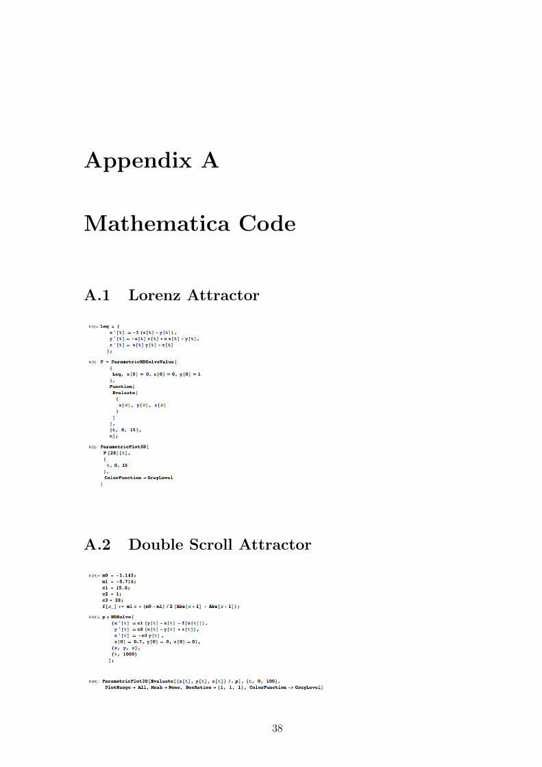
Appendix A
Mathematica Code
A.1 Lorenz Attractor
A.2 Double Scroll Attractor
38
An Exploration of Chaotic Behavior in Electrical Circuits
A.3 Matsumoto’s Double Scroll Attractor
A.4 Chua Oscillator, Failed
Chapter A Ryan O’Connell 39
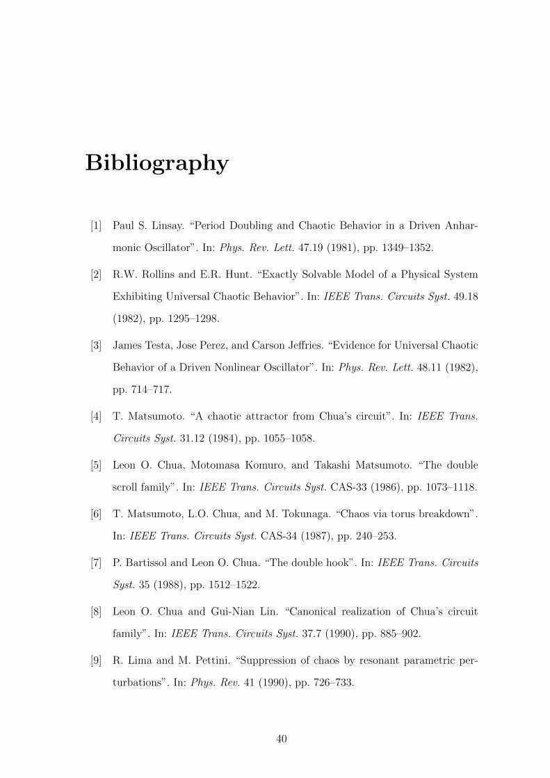
Bibliography
[1] Paul S. Linsay. “Period Doubling and Chaotic Behavior in a Driven Anhar-
monic Oscillator”. In: Phys. Rev. Lett. 47.19 (1981), pp. 1349–1352.
[2] R.W. Rollins and E.R. Hunt. “Exactly Solvable Model of a Physical System
Exhibiting Universal Chaotic Behavior”. In: IEEE Trans. Circuits Syst. 49.18
(1982), pp. 1295–1298.
[3] James Testa, Jose Perez, and Carson Jeffries. “Evidence for Universal Chaotic
Behavior of a Driven Nonlinear Oscillator”. In: Phys. Rev. Lett. 48.11 (1982),
pp. 714–717.
[4] T. Matsumoto. “A chaotic attractor from Chua’s circuit”. In: IEEE Trans.
Circuits Syst. 31.12 (1984), pp. 1055–1058.
[5] Leon O. Chua, Motomasa Komuro, and Takashi Matsumoto. “The double
scroll family”. In: IEEE Trans. Circuits Syst. CAS-33 (1986), pp. 1073–1118.
[6] T. Matsumoto, L.O. Chua, and M. Tokunaga. “Chaos via torus breakdown”.
In: IEEE Trans. Circuits Syst. CAS-34 (1987), pp. 240–253.
[7] P. Bartissol and Leon O. Chua. “The double hook”. In: IEEE Trans. Circuits
Syst. 35 (1988), pp. 1512–1522.
[8] Leon O. Chua and Gui-Nian Lin. “Canonical realization of Chua’s circuit
family”. In: IEEE Trans. Circuits Syst. 37.7 (1990), pp. 885–902.
[9] R. Lima and M. Pettini. “Suppression of chaos by resonant parametric per-
turbations”. In: Phys. Rev. 41 (1990), pp. 726–733.
40

An Exploration of Chaotic Behavior in Electrical Circuits
[10] Y. Braiman and I. Goldhirsch. “Taming chaotic dynamics with weak periodic
perturbations”. In: Phys. Rev. Lett. 66 (1991), pp. 2545–2548.
[11] R.N. Madan. “Observing and Learning Chaotic Phenomena”. In: Proc. 35th
Midwest Symp. Circuits Syst. 736-745 (1992).
[12] Leon O. Chua, Chai Wah Wu, and Anshan Huang. “A Universal Circuit for
Studying and Generating Chaos - Part I. Routes to chaos”. In: IEEE Trans.
Circuits Syst. 1 40.10 (1993), pp. 732–744.
[13] Robert C. Hilborn. Chaos and Nonlinear Dynamics: An Introduction for Sci-
entists and Engineers. New York: Oxford University Press, 1994.
[14] Chi-Chuan Hwang, Jin-Yuan Hsieh, and Rong-syh Lin. “A linear continuous
feedback control of Chua’s circuit”. In: Chaos, Solitons and Fractals 8 (1997),
pp. 1507–1515.
[15] S. Rajasekar, K. Murali, and M. Lakshmana. “Control of chaos by nonfeedback
methods in a simple electric circuit system and FitzHugh-Nagumo Equation”.
In: Chaos, Solitons, and Fractals 9 (1997), pp. 1545–1558.
[16] Tzuyin Wu and Min-Shin Chen. “Chaos control of the modified Chua’s circuit
system”. In: Physica D: Nonlinear Phenomena 164.1-2 (2002), pp. 53–58.
[17] Renato Mariz de Moraes and Steven M. Anlage. “Unified model and reverse
recovery nonlinearities of the driven diode resonator”. In: Physical Review E
68.2 (2003).
[18] Edward Ott. Controlling chaos. 2006. url: http://www.scholarpedia.org/
article/Controlling_chaos.
[19] Gaurav Gandhi and Tamas Roska Bharathwaj Muthuswamy. “Chua’s Circuit
for High School Students”. In: International Journal of Bifurcation and Chaos
(2007).
[20] Geoff Boeing. Chaos Theory and the Logistic Map. 2015. url: http : / /
geoffboeing.com/2015/03/chaos-theory-logistic-map/.
Chapter A Ryan O’Connell 41

An Exploration of Chaotic Behavior in Electrical Circuits
[21] Valentin Siderskiy. Chua’s circuit diagrams, equations, simlulations and how
to build. 2016. url: http://Chuacircuits.com.
[22] Population Growth. url: http://www.pspwp.pwp.blueyonder.co.uk/
starting-points/simulations-chaos/pop-growth.html.
[23] Sensitivty of Lorenz Equations. url: https://www.wolfram.com/mathematica/
new-in-9/parametric-differential-equations/sensitivity-of-the-
lorenz-equations.html.
42 Chapter A Ryan O’Connell