Portland State University Portland State University

PDXScholar PDXScholar

Dissertations and Theses Dissertations and Theses

12-14-1977

An Experimental Investigation of the Hole-drilling An Experimental Investigation of the Hole-drilling

Technique for Measuring Residual Stresses in Technique for Measuring Residual Stresses in

Welded Fabricated Steel Tubes Welded Fabricated Steel Tubes

Chau Mong Tran Portland State University

Follow this and additional works at: https://pdxscholar.library.pdx.edu/open_access_etds

Part of the Engineering Commons

Let us know how access to this document benefits you.

Recommended Citation Recommended Citation Tran, Chau Mong, "An Experimental Investigation of the Hole-drilling Technique for Measuring Residual Stresses in Welded Fabricated Steel Tubes" (1977). Dissertations and Theses. Paper 2574. https://doi.org/10.15760/etd.2571

This Thesis is brought to you for free and open access. It has been accepted for inclusion in Dissertations and Theses by an authorized administrator of PDXScholar. Please contact us if we can make this document more accessible: pdxscholar@pdx.edu.

AN ABSTRACT OF THE THESIS OF Chau Mong Tran for the Master of Science

presented December 14, 1977.

Title: An Experimental Investigation of the Hole-drilling Technique for Measuring Residual Stresses in Welded Fabricated Steel Tubes.

APPROVED BY MEMBERS OF THE THESIS COMMITTEE:

Wendelin H. Mueller, Ill,pairman

Ha_l'k Erzurp

~

Robert W. Rempfer

Among semi-destructive methods of measuring residual stresses

in elastic materials, the blind hole-drilling strain-gage method is

one of the best because it is simple, economical and accurate. It is

based on the measurement of strains disturbed by machining a small dia-

meter shallow hole in the test piece. The strains measured in three

known directions permit the determination of the direction and magnitude

of principal stresses and subsequently of any stress in any direction.

This thesis presents the investigation of residual stresses in

the longitudinal direction of a welded fabricated steel tube of 22 inch

diameter, relating to a series of holes drilled in one half of a

circular section of the tube. An initial assumption, substantiated

later, was the existence of a uniform field of residual stresses through

the thickness of the tube. Several methods for determining calibration

coefficients are documented. The values of longitudinal stresses once

computed are presented in a smooth curve. A straight line approximation

is reconnnended for use in further studies of the effects of residual

stresses on failure loads.

AN EXPERIMENTAL INVESTIGATION OF THE HOLE-DRILLING TECHNIQUE

FOR MEASuRING RESIDUAL STRESSES IN WELDED FABRICATED STEEL TUBES

by

CHAU MONG TRAN

A thesis submitted in partial fulfillment of the requirements for the degree of

MASTER OF SCIENCE in

APPLIED SCIENCE

Portland State University 1977

TO THE OFFICE OF GRADUATE STUDIES AND RESEARCH:

The members of the Committee approve the thesis of Chau Mong

Tran presented December 14, 1977.

Wendelin H. Mueller, III, Chairman

Ha~ Erzurum~

Arnold Wagner

Robert w. Rempfer

APPROVED:

Young~ad,~g\l.neering and Applied Science

I N LOVING MEMORY OF MY PARENTS,

OF MY PARENTS-IN-LAW, AND OF

MY FOSTER FATHER.

TO MY FOSTER MOTHER,

TO MY BROTHER,

TO MY WIFE,

TO MY CHILDREN,

TO MY CHILDREN-IN-LAW.

ACKNOWLEDGMENTS

This investigation was carried out under the supervision of

Dr. Wendelin H. Mueller. The author is deeply indebted to Dr. Mueller

for his continued help, leadership and guidance throughout the course

of this study. The author also wishes to express his grateful appre­

ciation to the Engineering and Applied Science Department, especially

the Civil-Structural Engineering Section.

The author would like to convey his warmest ~hanks to the other

members of his thesis committee: Dr. Hacik Erzurumlu, Dr. Robert

Rempfer and Mr. Arnold Wagner for their helpful comments and valuable

suggestions.

Also, much appreciation is due to Dr. Franz N. Rad for his advice

and suggestions. Special thanks are due to Mrs. Marjorie Terdal for

help and encouragement.

The author would like to extend his appreciation to Mr. Thomas

Gavin for his advice and encouragement and to Mr. Steve Barrett for

his help in computer programming.

The help of Mr. Steve Speer throughout the physical testing is

also acknowledged and appreciated. Thanks are also due to Mrs. Donna

Mikulic for typing this thesis.

Finally, the author would like to thank his wife, Mrs. Tran Thi

Ngo for her interest and encouragement throughout the author's graduate

work, his children and children-in-law for their encouragement.

TABLE OF CONTENTS

PAGE

ACKNOWLEDGEMENTS • • • • • • • . • • • • • • • • • • • • • • • • • • • • • • • • • • • • • • • • • • • • • • • • • • . iv

LIST OF TABLES . . . . . . . . . . . . . . . . . . . . . . . . . . . . . . . • . . . . • . . . . . . . . . . . . . . . . viii

. LIST OF FIGURES . . . . . . . . . . . . . . . . . . . . . . . . . • . . . . . . . . . . . . . . . . . . . . . . . . . . ix

LIST OF SYMBOLS .................................... • : ........ -. . . . . . xii

CHAPTER

I

II

INTRODUCTION .•••.••.•...••••••.••••.•••••••.••••••••••.• 1

1.1 Review of Literature............................... 1

1. 2 Objective of This Investigation.................... 4

1.3 Organization of the Report......................... 5

ANAL YT I CAL APPROACH •..•.••.•••....•.••••.•.•••••••.••.•• 7

2 .1 General Considerations............................. 7

2.2 Hole-4rilling Method............................... 8

2.2.1 2.2.2

2.2.3

2.2.4 2.2.5

Presentation of the Method Terminology of Stresses and Mathematical

Expressions Measuring strains using the strain

gage rosette Limit of strains for D/D0 • 1.0 Variation in residual stress field

2.3 Determination of calibration coefficients by experimental method................................ 15

2.3.1 Determination of calibration coefficients by the method of strain relaxation due to drilling

2.3.2 Determination of calibration coefficients by method of strain separation

vi CHAPTER PAGE

2.3.3 Experiment of tensioning a steel plate specimen for calibration

2.4 Computer Programs................................... 20

2.4.1 Calculation of cr1 and crz When Strains in 3 Directions are Known

2.4.2 Calculation of °L and crT When Strains in 3 Directions are Known

2.4.3 Calculation of q, and £T When Strains in 3 Directions are Known

III EXPERIMENTAL PROGRAM................... . • • . • • • . . • . . • • . . • • 23

VI

3 .1 Physical Tests . . . . . . . . . . . . . . . . . . . . . . . . . . . . . . . . . . . . . . 23

3.1.1

3.1.2 3.1. 3

Drilling Outside Holes a) Material and Gages b) Apparatus c) Experimental Set Up d) Validity of Results and Remarks Drilling Inside Holes Experiment of Tensioning and Drilling

Holes on a Steel Plate Specimen a) Material and Gages b) Apparatus c) Experimental Set Up

3.2 Test Results ........................................ 52

3.2.1 Results From Hole Drilling Experiment Evaluation of Results

a) Remarks b) Variation in stress field

3.2.2 Tensioning and Calibration Experiment a) Results of the Test b) Computation of the Modulus of elasticity c) Results from Method of Strain-Relaxation d) Results from Method of Strain Separation e) Summary of results f) Application of Calibration Coefficients

to Tube Data

BALANCE OF FORCES AND MOMENTS •.••...•••••.••••••.•••••••• 85

4.1 Balancing Forces and Moments of results using analytically derived calibration coefficients....... 85

4.1.1 Analytical Approach a) Pattern of longitudinal Residual

Stress Distribution

CHAPTER

v

REFERENCES

APPENDIX I

4.2

4.1. 2 4.1. 3 4.1.4

b) Area and Center of Gravity c) Application to Tube Data d) Dimensions and Values for Summation

of Forces and Moments

Flow Diagram Computer Program Results of the computer program

Evaluation of results ..............•..

SUMMARY, CONCLUSIONS AND RECOMMENDATIONS •...•.••••.••••••

5.1 SulilDlary of Results ................................. .

5.2 Conclusion . ........................................ .

5.3 Reconnnenda t ions .................................... ;

.........................................................

......................................................... APPEND IX I I ........................................................ .

APPENDIX III . ...................................................... .

APPENDIX IV ........................................................ APPENDIX V ........................................................ APPENDIX VI ........................................................ APPEND IX VI I .........................•.....................•...•...•

APPEND IX VI I I .•....•....•..•••....•...•...••...••..•.•.••.•••.•..•..

APPENDIX IX ........................................................ APPENDIX X ......................................................... APPENDIX XI . ...................................•.....•........•.....

vii

PAGE

105

107

107

108

110

113

115

119

121

123

125

127

135

139

147

154

160

TABLE

3.1

3.2

3.3

3.4

3.5

3.6

3.7

3.8

3.9

3.10

3.11

3.12

LIST OF TABLES

Experiment of Outside Hole Drilling Results for Hole 1.

Experiment of Outside Hole Drilling (continued)

Experiment of Outside Hole Drilling Data and Results for 11 Holes.

Experiment of Inside Hole Drilling Results for Four Holes

Values of factors of proportionality

Data from a non-uniform stress field

Results of application to tube data

Experiment of Tensioning and Calibration Data from Strain-Relaxation .Method

Experiment of Tensioning and Calibration Data from Method of strain separation

Values of 4A and 4B computed by curves from Figure 2.3

Recapitulation of 4A and 4B Values

Results with Computed Data Reduction Coefficients

3.13 Results from Method of Strain-Relaxation Due to Drilling

3.14 Results from Method of Strain separation

4.1 Results of Force and Moment Balance

PAGE

53

54

56

58

62

64

67

68

69

73

75

78

80

83

106

FIGURE

2.1

2.2

2.3

2.4

2.5

3.1

3.2

3.3

3.4

3.5

3.6

3.7

3.8

3.9

3.10

3.11

3.12

3.13

3.14

3.15

3.16

3.17

3.18

3.19

LIST OF FIGURES

Radial and tangential strains

Position of gage with respect to principal stress

Data reduction coefficients 4A and 4B

Strain-relaxation due to drilling

Strain separation

Steel tube

Strain gage rosette

Milling guide

Strain indicator

Strain indicator, rear view

Location of hole section

Position of drilled holes

Rosette pattern enlarged

Orientation or rosette gages

Adjustable swivel feet

Milling bar

Drilling set up

Drilling under action

Set up for drilling inside hole

Cementing swivel feet

Alignment set up before drilling

Inside hole drilling under action

Shape of the steel plate specimen and position of gages

Material Testing System (MTS)

PAGE

9

9

13

19

19

25

.25

28

28

29

31

31

33

33

35

35

36

36

39

39

40

41

42

44

FIGURE

3.20

3. 21

3.22

3.23

3.24

3.25

3.26

3.27

3.28

3.29

3.30

3.31

4.1

M T S with load cell

Gage A for a residual stress check

Hole in gage A under drilling

Setting test piece in the jaws of the MTS

Hole in gage B under drilling

Reference gage at left hand side

Strain separation for Direction 1 with numerical application

Strain relieved vs depth

Curve of initial values of measured longitudinal residual stresses

Curve of longitudinal residual stress.es recalculated with new data reduction coefficients

Curve of longitudinal residual stresses computed from strain-relaxation method

Curve of longitudinal residual stresses computed from the method of strain separation

Pattern of distribution of longitudinal residual stresses

4.2 Segmental division for preparing data for the computer program

4.3 Area and center of gravity. Case 1.

4.4

4.5

4.6

4.7

4.8

4.9

4.10

Case 2

Case 3

Case 4

Case 5

Case 6

sketch of a three dimensional representation of the tube and an element of area of forces

Cross-section of the tube

x

PAGE

44

45

45

47

49

49

51

59

77

79

82

84

86

88

90

90

91

91

93

93

94

95

FIGURE

4.11 Sketch of a volume of forces

4.12 Flow diagram

5.1 Curve of residual stresses by hole-drilling method (solid line) and curve by method of sectioning (dashed line)

5.2 Ross and Chen simplified curve by sectioning method and simplified curve by hole drilling method

A.6.1 Stress Mohr's circle

A.7.1 Strain Mohr's circle

A.11.1 Polygonal line and smooth continuous curve . representing residual stresses, Table 3.11, Case 1

A.11.2 Polygonal line inscribed in continuous curve to define elementary areas of forces

A.11.3 Conversion of tube data to input for the computer program

xi

PAGE

95

99

109

112

127

136

161

163

165

LIST OF SYMBOLS

4A Data reduction coefficient or calibration coefficient

4B Data reduction coefficient or calibration coefficient (for minimum principal stress)

D Difference of strains, E - E a c

d Outside diameter of the steel tube

d1

Inside diameter of the steel tube

E Modulus of elasticity

I Moment of inertia

M Bending moment at first yield y

P Axial load

P Axial load causing complete yielding of the cross-section y -

R Distance of the gage to hole center

R Radius of the drilled hole 0

r R/R , ratio of R to R 0 0

S Sum of strains, E + E a c

s Section modulus

t Thickness

a

8

E a

Eb

E c

Angle of longitudinal stress to principal stress o1

Angle of direction (gage) a to principal stress o1

Strain measured by gage a

Strain measured by gage b

Strain measured by gage c

EL Longitudinal strain

ET Transverse strain

a1

Principal stress, maximum

xiii

a Principal stress, minimum 2

aL Longitudinal residual stress

aT Circumferential or transverse residual stress

a Yield stress y

CHAPTER I

INTRODUCTION

1.1 REVIEW OF LITERATURE

In many occurrences, one of the predominant factors contributing

to structural failures and fatigue in welded parts, pipes, rolled

structural shapes and finished structures, is the residual stresses

which existed in the part before being put into service. These

stresses are introduced either by the initial imperfecti~ns in fabri­

cation or during the manufacturing processes due to the operations of

casting, molding, laminating, heat treating, cold or hot rolling,

machining or welding. In other instances, residual stresses can

appear due to installation procedures or the dead weight of the

structure. In general, residual stresses tend to reduce the strength

in stability, fatigue and fracture (7, 13, 14); in some situations,

however, their existence might improve the strength (13, 14). Conse­

quently, knowledge of the distributions and magnitude of the residual

stresses is a necessary prelude to any analytical investigation of

the effects of these stresses on the behavior of the structure.

The directions and magnitudes of these stresses can be determined

by several methods:

- Methods termed "destructive" consist of removing metal by

machining, slicing (5, 7) grinding or etching and measuring elastic

strains of the remaining section.

In 1888, Lalakoutsky (7) reported on a "sectioning method"

to determine longitudinal stresses in steel bars by slicing longitu-

2

dinal strips from the bar and measuring their change in length. The

other methods are based on similar principles. That is the internal

stresses are relieved or changed when the specimen is reduced to strips

or pieces of smaller cross-section. The test piece submitted to the

experiment of one of these methods, is unusable in its original con­

figuration and thus the method is termed destructive.

Non-destructive or x-ray methods are based on the principle of

modification of the texture of metal grains revealed by x-rays. The

results are correlated to the texture of the same metal under known

stress conditions. Internal stresses present in the metal piece are

finally determined.

Semi-destructive methods consist of machining a shallow hole

in a test piece by means of a rotating cutter or an abrasive jet, and

of measuring the strains disturbed in three directions by a strain-gage

rosette: the stresses present in the test piece, for any direction

around the hole, are computed from these strains.

Because of the complexity of their use, the slicing techniques

have become less acceptable.

Using x-ray does not lend itself to field conditions and stresses

can be detected only in the surface layer to a depth of one thousandth

of an inch.

The two hole-drilling methods attempt to minimize the disadvan­

tages of the previous discussed methods.

The "Abrasive Jet Machining" method consists of directing a con­

trolled stream of gas containing fine abrasive particles against a

workpiece to chip away tiny particles of material making a small hole.

3

The strains relieved are measured by means of a strain-gage and internal

stresses relaxed around the drilled hole can be calculated. However,

because the "Abrasive Jet Machining" method (2) requires costly equipment­

the hole-drilling or hole-relaxation method., consisting of drilling a

hole in the test piece by means of a rotating cutter and of measuring

the strains relieved with a strain-gage, was used in this study. Both

are termed "semi-destructive", because the amount of metal removed is

small. The part itself once drilled for the disturbed strains can be

repaired by means of a rivet or a plug and recovers the integrity of

its strength and properties.

The drilling method was first conceived by G. Sachs (6) who,

in 1927, worked with specially shaped pieces (e.g., those with round

or rectangular cross-sections). In 1932, Josef Mathar in Germany (1,3)

developed the technique and measured the deformations around the -drilled

hole by means of a mechanical extensometer. His apparatus has been

subject to criticism, because the vibrations during drilling cause the

strain readings to be unsteady and irregular. The use of the method

developed by Mathar is restricted to cases where the stresses are con­

sidered to be uniform through the thickness.

In 1948, Soete in Belgium (1) improved the technique and extended

its use to cases of non-uniform stress field.

During the evolution of the hole-drilling technique the strains

relieved were at first measured by an extensometer (1) then by some

photoelastic materials bonded to the specimen surface or by a brittle

lacquer sprayed on its surface (2,10). Finally, in the present time,

bonded resistance wire strain gages constitute the most widely used

4

process of strain measurement (2,10,12). The combined method - hole

drilling and strain gage - finds its use in most work, because of its

simplicity, ease of strain measurement and stress calculation and its

higher precision. In fact, it has been proven in a specific job that

the hole-drilling method needs only 10 man hours, where as the layer

removal method requires about 70 to 80 man hours (1), the former saves

at least 85 per cent of labor and time.

In spite of its numerous advantages, the hole-drilling method

shows two relatively unfavorable conditions:

a) Difficulty of obtaining a perfect alignment of the drilled

hole with respect to the strain gages (problem of centering the drill

bit in a gage rosette).

b) Spot residual stresses introduced during drilling.

The first disadvantage can be avoided by using a commercial fix-

ture: a precision milling guide capable of centering the hole to the

center of the rosette within ±0.001 inch.

A method of determining the effect of the spot residual stresses

~ caused by drilling, described in detail in -paragraph 2.3.1 overcomes

the second shortcoming. The spot residual stresses introduced during

drilling, although measured at the same time by the strain gage, are

separated from the stresses of interest by the use of calibration co-

efficients.

1.2 OBJECTIVE OF THIS INVESTIGATION

The purpose of this investigation is to study longitudinal

residual stresses present in a welded fabricated steel tube, to

determine their magnitudes and distributiops along a semi-circular

cross-section and to check the correctness of measurements bya test

of statical equilibrium of the stress distribution. The tube chosen

was 5/16 inch thick, 22 inches in diameter and 6 feet long.

The following outlines the two major steps in determining re-

sidual stresses:

1) Drilling holes oh the outside and inside surfaces, in one I

half of a circular section1 of the tube, two feet from the edge, then

measuring the strains by m!eans of strain gage rosettes, calculating

the corresponding longitudjinal stresses using the calibration coeffi­

cients determined in Step 12, and plotting these stresses in a curve.

5

2) I Performing exper1iments of calibration. The first one is con-

ducted according to a cal~bration process of strain-relax~tion due to

drilling: a plate specim; n is submitted to a known applied tension,

then a hole is drilled in !the plate. The strain due to the applied

stress and the strain induced by the drilling are measured. This I

calibration yields the first pair of calibration coefficients. I

The second experime*t is carried out according to a calibration

process of separating str,ins and consequently the induced stresses

and applied stresses. This experiment gives the second pair of calibra-

tion constants.

In the calibration study, a steel plate was used h$ving the same

general characteristics as the steel tube.

1 . 3 ORGANIZATION OF THE REPORT

The following is a documentation of longitudinal residual

. ~ '

stresses present in a welded fabr i ca ted stee l t ube.

The hole-drilling me t hod was used in the expe r i".Ilen t: o :": dr iU.i nf,

outside and inside of a semi-circular section of a full steel t ube .

Calibration coefficients we~e determined through experiments of pr e­

loading a steel plate specimen.

A procedure is presented which separates stresses introduced

by the drilling process.

The results are shown as a stress distribution around the circum­

ference of the tube. An i ndependent check of translational and rotation­

al equilibrium is presented. A stress distribution is recommended for

use in a study of the effect of residual stresses on failure loads of

fabricated steel tubes.

CHAPTER II

ANALYTICAL APPROACH

2.1 GENERAL CONSIDERATIONS

As the investigation is carried out on a welded cylindrical

steel tube, it is appropriate here to describe the process by which

welded fabricated steel tubes are commonly made. Usually, before

welding, several cycles of cold-rolling of a flat plate are repeated

until the two opposite edges come together to form a cylinder or "can".

A can is then completed by welding along the longitudinal seam. The

length of the can is usually limited to 10 feet by this manufacturing

process, but several cans can be welded together end-to-end to yield

the desired length .

A possibility of longitudinal weld tearing in a finished member

when loaded, is avoided by staggering the weld between cylinders making

the weld in one can 180 degrees out-of-phase to the weld in the next

can.

This manufacturing process generally introduces:

a) Initial residual stresses from the flat plate before forming

the "can" (5,14).

b) Circumferential residual stresses by repeated cold-rolling

(5).

c) Longitudinal residual stresses due to longitudinal welding

(S)(Shrinkage during cooling).

d) A bending moment on the cross-section of the wall of the

8

(3) because it is possible that the edges of the rolled plate do not

meet exactly, thus requiring some "pulling together" of the edges prior

to or during the welding operation (incomplete "spring back")(S).

Among these stresses, measurement of longitudinal residual

stresses is the main objective of this analysis.

2.2 HOLE-DRILLING METHOD

2.2.1 Presentation of the method. The measurement of residual stresses

cannot be performed by conventional surface techniques such as photo-

elastic coatings or strain gages, because the measuring device ignores

the past story of the parts. It measures strain after it is bonded

to the part.

For this investigation, the hole-drilling method was chosen

for use in determining the "locked-in" stresses. The stress field

being disturbed by drilling, stresses are relaxed around the hole

and relieved strains are measured.

2.2.2 Terminology of stresses and mathematical expressions. When a

hole of smaller diameter (d = 2R ) is drilled in a part subjected to 0 .

residual stresses, a strain relaxation occurs. If there is only one

stress o1 , the strains relieved at a point P from a distance R of the

center A of the hole are called radial strain Er and tangential strain

Et (10), in Figure 2.1.

2 4 2 Er= -o1 (1+µ)/2E(l/r -3 cos 2a/r + 4 cos 2a/((l+µ)r )) (1)

2 4 2 ~= -o1 (1+µ)/2E(-l/r +3 cos 2a/r - 4 cos 2a/((l+µ)r ))

t

'_L __ , _~---L 1 I e ~ I -l ,:;:· -... I

I ' -~ I I R.! / cJ.°'~ ,5-

1

,- -~,',,·.Jt -:--1--• I I

.____-~-~---J-Figure 2, 1 Radial and tangential strains

I

\

,

,, '

------ -"i

-1- .-

Figure 2,2 Position of gages with respect to principal stress o-1 •

9

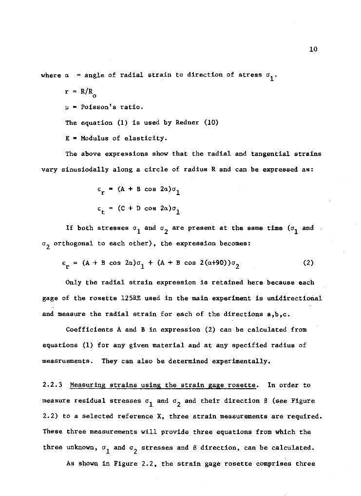
where a = angle of radial strain to direction of stress cr1 •

r = R/R 0

µ = Poisson's ratio.

The equation (1) is used by Redner (10)

E = Modulus of elasticity.

10

The above expressions show that the radial and tangential strains

vary sinusiodally along a circle of radius R and can be expressed as:

£r = (A + B cos 2a)a1

£t = (C + D cos 2a)a1

If both stresses cr1 and o2 are present at the same time (o1 and

o2 orthogonal to each other), the expression becomes:

£r = (A+ B cos 2a)o1 + (A + B cos 2(a+90))o2 (2)

Only the radial strain expression is retained here because each

gage of the rosette 125RE used in the main experiment is unidirectional

and measure the radial strain for each of the directions a,b,c.

Coefficients A and B in expression (2) can be calculated from

equations (1) for any given material and at any specified radius of

measruements. They can also be determined experimentally.

2.2.3 Measuring strains using the strain gage rosette. In order to

measure residual stresses o1 and o2 and their direction· B (see Figure

2.2) to a selected reference X, three strain measurements are required.

These three measurements will provide three equations from which the

three unknown, o1 and o2

stresses and B direction, can be calculated.

As shown in Figure 2.2, the strain gage rosette comprises three

11

separate gages in directions a,b,c spaced 45 degrees apart, on a

radius R. The strains can be established from equation (2) by letting

the angles:

a.a = 13 ab = 13 (). - 8 + 90° c

Solving for stresses, one obtains (Derivation of equations (3)

is given in Appendix I):

al ((A+B cos 213)£ - (A-B cos 28)£ )/4AB .Qos 213 a c ·-

a2 = ((A+B cos 213)£c - (A-B cos 213)£a)/4AB ,oos. 28 (3)

Tan 28 • (£ - 2£b + £ )/(£ - £ ) a c a c

The equations are for a hole drilled in a macroscopically

homogeneous, isotropic material subjected to a biaxial stress.

Equations (3) provide good results when gages a and c ar~

approximately positioned along principal stresses (10). But if the

directions are grossly misjudged and gages a and c give the largest

spread, the following equations (4) provide better results (Derivation

of equations (4) given in Appendix II):

a = 1

(A + B sin 213)£a - (A - B cos 28)£b

2 A B (sin 213 + cos 213)

(A+ B cos 213)£b - (A - B sin 213)£a a =

2 2 A B (sin 213 + cos 213)

(4)

Equations (3) can be rewritten in the following _form to simplify

the numerical calculations (lO)(Derivation of equations (3a) is given

in Appendix III)

12

o1

= S/4 A + D/4 B cos 2S

(3a)

with

where

o2 = S/4 A - D/4 B cos 2S

Tan 2$ = (S - 2£b)/D

s = £ + £ a c

D = £ - £ a c

The coefficients 4A and 4B can be computed from equation (1)

or obtained from curves in Figure 2.3; these curves established by

S. Redner (10) yield one pair of values of 4A and 4B for one value

of r = R/R . In this study, they were also determined experimentally. 0

Each system of equations (3),{3a) and (4) can be used- to compute

the magnitudes and directions of the principal stresses. However,

for the case of this investigation, the system of equations (3a) is

most often applied because of their simplicity.

A computer program using equations (3a) to calculate the

directions and magnitudes of the principal stresses, when the strains

£ , £b and £ are known, is given in Appendix IV. a c

Generally the directions of the principal residual stresses

calculated do not coincide with the longitudinal and circumferential

directions of the tube. A graphical method using a stress Mohr's

circle (11) permits the orientation of the longitudinal and circum-

ferential residual stresses.

When the strains in the directions of gages a, b and c are

known, a graphical solution using a strain Mohr's circle (11) allows

the calculation of the longitudinal and circumferential strains

-5 ( 1()'"8)

-4

I -J l

-2

-1

0

4A l4B

2.2

11gure 2.J Data reduction coefficients 4A and 4B

4.A

2.4 2.6 2.8 J.O J.2 r=R/Ro ~ w

14

(see Appendix VII).

A series of computer program presented in section 2.4 constitutes

a second method for solving the above mentioned problems (see Appendices

VI and VIII).

2.2.4 Limit of strains for D/Do = 1.0. As mentioned previously, the

hole-drilling method is based on the fact that drilling a hole in a

stress field disturbs the equilibrium of the stresses, thus causing

measurable strains at the surface of the part, adjacent to the hole.

Previous investigators have found that the deformations of the surface

in a thick test piece, approach a limiting value. This is because the

stresses relieved from the removal of the metal, at some distance below

the surface will have no effects on the deformations at the surface.

It has been found that this limiting value occurs at a hole depth varying

from one to two times the hole diameter (1). Mathar (6) found this

limit to be 1.5 to 2, while Bush, Kromer (2) and Redner (10) suggested

1.0.

In this investigation, it was found that little change in the

strains occurs after a hole depth to diameter ratio of 1.0 is reached.

For convenience, it will be shown in Chapter III.

2.2.5 Variation in residual stress field. An assumption has been made

that the residual stresses existing in the tube are uniform through its

thickness. This assumption will be numerically substantiated in section

3.2.1.b.

At this time, the following observation about the distribution of

residual stress is noted.

According to S. Redner (10), the criterion of a uniform stress

field is:

When the residual stresses are uniform in depth, the strains in the immediate vicinity of the hole are fully relieved (the curve reaches an asymptotical value) when the depth equals approximately one diameter of the hole.

In this study, it was found that strains relieved were small

15

for the first layers of material, but increased with depth. When the

hole depth reached the value of hole diameter, strains attained their

maximum and when plotted remained parallel to the horizontal axis.

The quasi-stationary values of the stresses computed for several

depth values close to the constant diameter value will be shown in

Chapter III a substantiation of the above assumption.

2.3 DETERMINATION OF CALIBRATION COEFFICIENTS BY EXPERIMENTAL METHOD

The hole-drilling or hole-relaxation method of measuring residual

stresses is based on the measurement of strains distributed by machining

a small hole in the test piece. A theoretical solution for the strain

at any point on the surface of a drilled hole is not known and further-

more the relaxed strain is not uniform across the surface of the part.

A strain gage at best can measure the average strain across the area

it covers. Because of these limitations, most investigators believe that

a calibration procedure is necessary. Calibration operations consist

of applying known stresses to a test piece and measuring corresponding

strains. These known stresses and strains permit the establishment of

calibration coefficients which can be used in similar experiments to

calculate stresses when the strains relieved are known. In this in-

vestigation, results are presented using calibration coefficients obtained

16

by: a) theoretical calculations, b) published literature, c) experi­

mental work performed as part of this research.

2.3.1 Determination of calibration coefficients by the method of

strain relaxation due to drilling. This method consists of computing

the strain relaxed when a hole is drilled in a steel plate subjec~ed

to a known state of stress. In this method no account is made for

stresses induced by drilling.

The test set up is simple. A steel plate having a shape shown

in Figure 3.18 is installed in a testing system capable of applying

a tension force.

The following presents the major steps in this method:

1) A known tension (for example a tension giving a stress

a1 = 0.50 FY) is applied to the plate and strain Ea is

measured by a strain gage rosette B; Ea is the strain

due to the known force. Plot point a in Figure 2.4. (Note:

no hole has been drilled as yet.)

2) The tension is released. The strain reading comes back to

zero. A hole is drilled to a depth equal to the hole dia­

meter. There is another strain reading, but it is reset

to zero. The same tension is reapplied to the plate and a

new strain Eb is read and recorded; Eb is the total strain

due to the application of the force and the existence of the

drilled hole. Plot point b (strain Eb' stress a1) in

Figure 2.4.

3) The strain-relaxation 6E is the difference between the two

measured strains Ea and Eb.

17

As all strain readings have been zeroed before and after drilling,

the influence of any unknown residual stresses in the test plate is

eliminated. Their effect has been eliminated by using the experimental

procedure outlined above. All readings were zeroed before the force

was applied. As the known force is applied before and after drilling,

only the effects of the applied load and any stresses induced by

drilling are recorded.

This calibration method yields a pair of calibration coefficients

4A and 4B, their computation will be shown in Chapter III.

2.3.2 Determination of calibration coefficients by the method of

strain-separation. The second method of determining the calibration

coefficients separates the unknown stresses induced during the drilling

process.

It has been found that, during the drilling operation, signifi­

cant stresses are introduced in a general specimen by drill bits or

rotating cutters. According to Bush and Kromer (2), their magnitude

can be of the order of ±10000 psi. Now the change in strain introduced

by drilling a hole in any test piece when the latter is under load, is

a function of initial residual stresses, spot stresses induced by

drilling and applied stresses. Therefore, for an accurate calibration,

it is necessary to isolate the values of existing unknown residual

stresses in our test plate from stresses induced by drilling and from

those caused by our applied loads.

The test set-up is similar to the previous method but there are

some differences in making readings and computing strains. The same

test plate is installed in a testing system capable of applying a

18

tension force. The experimental procedure is as follows:

1) Before drilling, zero strain indicator. Apply a known load

(a1 = 0.40 FY) to the specimen. Record the strain E from a

the strain indicator. Plot point a of Figure 2.5.

2) Maintaining the stress a1

. A hole is drilled to the desired

depth. Record the corresponding strain Eb. Plot in the same

graph point b (Eb,a1).

3) Reduce the magnitude of stress to a2 (a 2 = 0.10 Fy) and

record the corresponding strain Ed. Plot point d(Ed,o2).

Locate point c, which is the intersection of line oa and

a line through d parallel to the strain axis (see Figure 2.5).

4) Extend line bd cutting the strain axis at point e (graphical

interpolation). £ is the strain with no load on the plate. e

As there is no load applied, the segment oe represents the

strain due to initial residual stresses and spot stresses

introduced by the drilling operation.

5) Referring to ordinate o1 , the segment ab represents the

difference of two strains Ea - Eb ~ 6ET which is the strain­

relaxation due to drilling under applied stress cr1 • 6£T is

the sum of two strains: 1) strains due to drilling effects

and unknown residual stresses existing in the plate and 2)

strains due to applied stress. From O, a parallel line to

eb is drawn cutting ab at b'. The segment bb' parallel and

equal to eo represents the strain due to drilling effects

and unknown residual stresses in the plate (6ER). The segment

b'a represents the strain due to the applied stress cr1 (6E1).

~ I - A ~, J •

0 Eb AE

Ea

e..=strain due to 61

E. b=Strain due to 6'1 and hole drilling

Ae. =Strain relaxed due to drilling

€

Figure 2,4 St.rain-relmt.1on du. to drU.llng

~·I b b' a

/1 /1 /1 Ae.a •Strain due to r•ai-

dual at.res••• and drilling etf ect

AE- I Er-Total strain due to

drilling effect ~E'T-~~ and applied 6"1

ile=Strain due to applied 6'1

et:. V" I ET =Ea - Eh~ E

Figure 2.5 St.rain aeparat.1on

19

20

Finally As1 is the strain eaused by the applied stress o1 .

6) At ordinate o2

, dd' parallel and equal to eo, represents

the strain due to drilling effects and unknown residual

stresses, and the segment d'c is the strain due to the applied

load o2 .

7) The above strain- relaxation has been obtained from a known

applied stress for a determined direction. In the case of

the gage rosette, it is necessary to calculate the strain­

relaxation for three different directions (a,b,c, 45 degrees

apart) under an uniaxial load.

2.3.3 Experiment of tensioning a steel plate specimen for calibration.

The purpose of this experiment is to determine the modulus of elasticity

of the steel of the plate, to check the existence of initial residual

stresses and stresses induced by drilling and finally, to determine

the calibration coefficients, first by the method of strain-relaxation

due to drilling, then by the method of strain separation.

Experimental set-up and results are described in detail and

illustrated with numerical values in Chapter III, sections 3.1.3 and

3.2.2.

2.4 COMPUTER PROGRAMS

In this part, three computer programs will be presented pertain­

ing to 1) the calculations of principal stresses, 2) of longitudinal

and circumferential stresses and 3) of longitudinal strain, when

radial strains in three directions (gages) a,b,c are known. Two more

computer programs will be discussed relating to force and moment

: .•..

21

balance before and after calibration.

As the system of the actual longitudinal residual stresses is

in equilibrium in the tube, the summation of forces and moments with

respect to an axis must equal zero. The first program computes the

balance of forces and moments of measured longitudinal residual stresses.

The second program deals with the balance pertaining to residual stresses

recalculated using calibration coefficients.

2.4.1 Computer program for calculating principal stresses a1

and a2

when strains in directions a,b,c are known. Calculations are based

on equations (3a):

with

a1 = S/4A + D/4B cos 26

a2

= S/4A - D/4B cos 26

Tan 26 = (S - 2£b)/D

s = £ + £ a c

d = £ - £ a c

These equations are used by Redner (10).

The computer program is shown in Appendix IV.

(3a)

2.4.2 Computer program for calculating longitudinal and circumferential

stresses when strains in three directions a,b,c are known. In this

program, the equation of a Mohr's circle constructed with principal

stresses is established. The equation of the straight line represen-

ting both longitudinal and circumferential directions is also computed.

The abscissas of the points of intersection between the line and the

:·o1 · ..

circle will be the longitudinal and circumferential stresses. (see

Figure A.6.1).

The computer program is presented in Appendix VI.

22

2.4.3 Computer program for calculating longitudinal and circumferen­

tial strains when strains in three directions are known. In this pro­

gram, the equation of a strain Mohr's circle is established. Also

computed is the equation of the line of the longitudinal strain

direction which is the same for the circumferential strain direction.

(The angle between longitudinal and circumferential direction is 90

degrees for the tube; but this angle is double and equals 180 degrees

in Mohr's circle.) The abscissas of the points of intersection between

the strain Mohr's circle and the line, will be the longitudinal and

circumferential strains. (See Figure A.7.1)

The computer program is presented in Appendix VIII.

CHAPTER III

EXPERIMENTAL PROGRAM

This chapter documents the testing procedure and presents the

numerical results of the laboratory tests.

Laboratory tests consist of experiments of drilling outside and

inside holes in the steel tube and of an experiment of tensioning a

steel plate specimen for calibration.

3.1 PHYSICAL TESTS

The first experiments consist of drilling a series of eleven

holes on the outside surface of a welded fabricated steel tube.

3.1.1 Drilling holes on outside surface.

A) Material and gages.

istics:

1) The steel tube specimen used has the following character-

Length: 6 feet

Outside diameter: 22 inches

Thickness of wall: 5/16 inch

Section modulus: 118.79 cubic inches

Yield axial load: 870.8 kips

Bending moment at first yield M : 4859 in. kip y

A-36 American made plate

The steel used in the tensioning experiment has the following

specifications:

Conform to ASTM-36.75

Yield strength: 40.90 ksi

Ultimate strength: 61.50 ksi

Ultimate strength: 61.50 ksi

Modulus of elasticity: 29 000 ksi

Chemical analysis: Carbon: .14%

Manganese: .67%

Phosphor: .009%

Sulfur: .018%

Silicium: .22%

2) Strain-gages used are of two types:

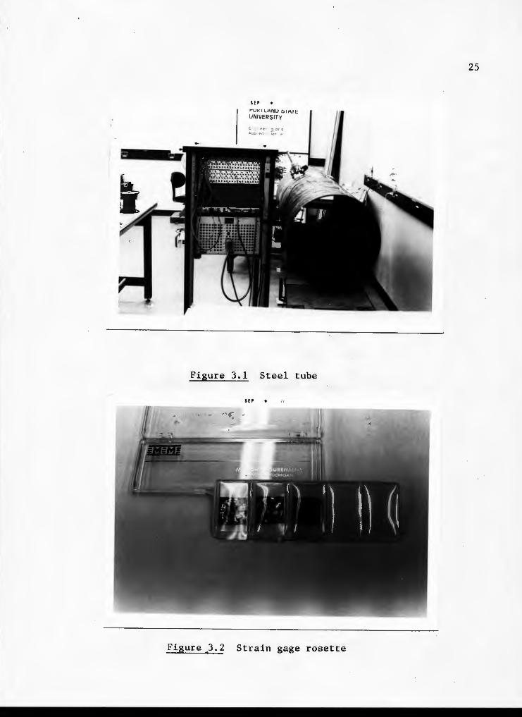
a) Rosette 0.125" (see Figure 3.2)

Gage type: EA .06-125 RE-120

Resistance in ohms: 120.0 ± 0.2%

Lot number: R - A 35 AD 48

Quantity: 5 gages per box

Option: S

Gage factor at 75°F: Nominal 2.03 + 1.0%

;·,,; · ..

Manufactured by Micro-Measurement M-M, Romulus, Michigan

This rosette is used with a drill bit of 0.125 inch to drill

holes of 0.125 inch diameter.

b) Rosette 0.062"

Gage type: EA . • 06-062 RE - 120

24

This resistance strain gage has specifications similar to those

of Rosette 0.125 in. except for its smaller dimensions and is used

for holes 0.062 in. in diameter.

SEP

P"'Ul'(IL'°'IV U ~IP.It

UNIVERSITY

Figure 3.1 Steel tube

SEP 71

Figure). 2 Strain gage rosette

25

26

B) Apparatus. T

1) Milling guide.

As mentioned previously, the difficulty of obtaining a good

alignment of the bored hole with respect to the gages can be overcome

by the use of a precision milling guide (see Figure 3.3).

The apparatus used in this experiment is a RS-200 special milling

guide (12) capable of allowing an alignment within ±0.001 inch of the

rosette center and insuring the concentricity and guidance of the milling

bar.

This guide is supported by a rigid body adjustable in two ortho­

gonal directions. The body is easily attachable to curved or flat

surfaces by means of an adjustable swivel tripod. When the gage is

cemented to the test piece, alignment is realized by putting the micro­

scope into the guide and centering the guide over the center of the gage

rosette by acting adjusting screws. When alignment is done, the micro­

scope is removed and the milling bar armed with rotating cutter is intro­

duced into the guide. The cutter currently used is of 0.125 in. diam-

eter.

According to Vigness and Rendler (4), end mills are normally

equipped with cutting edges on the end and side of the mill. The mill

will cut either with an axial or lateral feed motion. But, in 1966,

Greenweld and Rendler (10) made a complete and valuable study on this

matter and found an optimum shape for the drilling tool, insuring that

the boring progresses in a straight line, without side pressure or

friction at the non-cutting edge. This shape of drill bit has been

applied to the equipment used in the present experiment and allowed a

27

smooth drilling without side pressure or side friction.

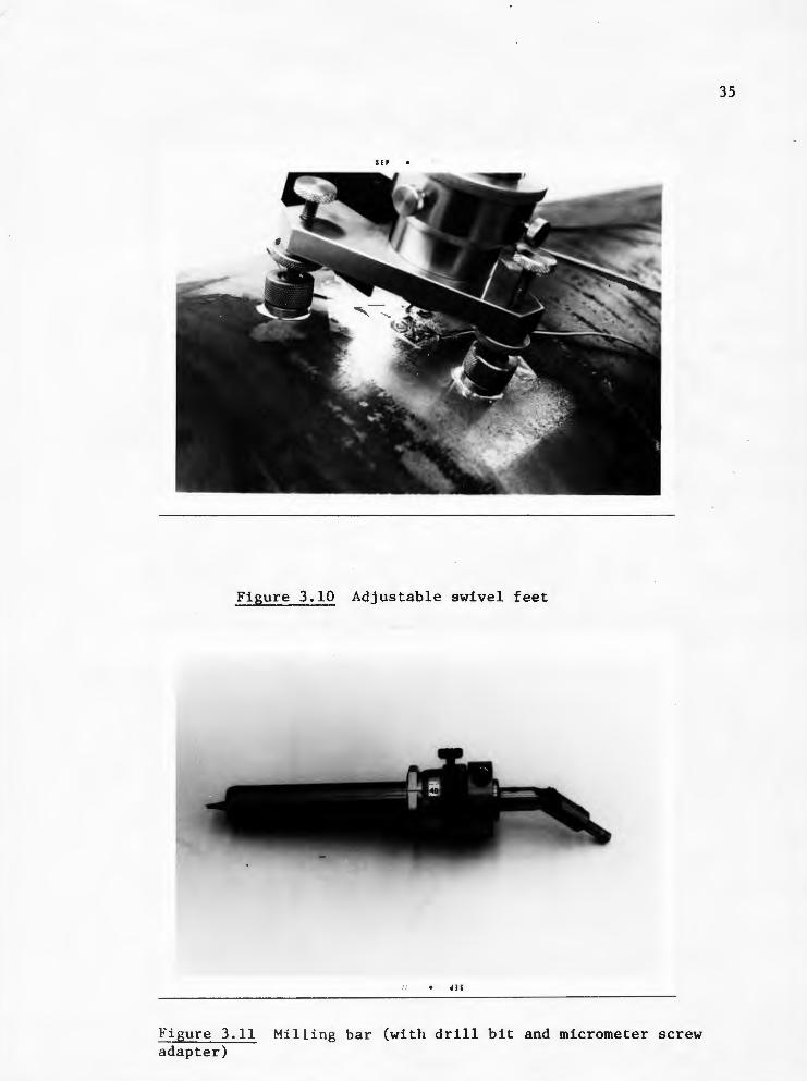
The milling bar is also equipped with a special micrometer screw

adapter to allow drilling in small increments in depth (generally 0.01"

per increment). After drilling, the diameter of the hole is measured

by the micrometer inside the microscope. This measured diameter is

necessary to compute the ratio r = R/R distance of the gage to the 0

center, to radius of the hole, to determine the data reduction coeff-

icients 4A and 4B leading to the computations of the principal stresses.

2) Strain indicator.

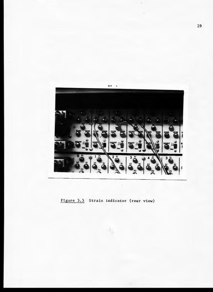
After the installation of the rosette, its three gages

are soldered to six wires (one pair of wires to one gage) connected

to the strain indicator (see Figures 3.4 and 3.5). The gage factor

is set up to the required value (2.03 for the EA .06-125 RE - 120

Rosette) and when the reading is reset to zero the test should yield

a reading of ±3 400 microstrains for each gage connected to the strain

indicator.

C) Experimental set up

The experimental set up comprises the following operations:

1) Location of holes, marking.

The longitudinal residual stresses were assumed to be

symmetric with respect to the dimetral plan passing through the longi-

tudinal weld. Therefore only the investigation of the stresses on a

semi-circular section of the tube was considered. A section two feet

from the edge (see Figure 3.6) has been defined and the holes were

drilled on a semi-circular section commencing from the weld (see

Figure 3. 7).

Figure 3.3 Milling guide

Figure 3.4 Strain indicator

29

SIP

Figure 3.5 Strain indicator (rear view)

30

Eleven holes were drilled and located from the weld as follows:

Hole Angle from weld

1 45°

2 90°

3 135°

4 180°

5 22°30

6 67°30

7 112°30

8 157°30

9 near weld

A 11°15

B 33°45

Each hole is marked with a sharp steel blade on the wall of the

pipe, strongly enough to leave a faint sign of a cross even after sanding,

but not so strongly as to create extraneous residual stresses in the

tube.

2) Cleaning the area ready for cementing the gages and the

swivel feet for mounting the milling guide.

-Sanding. As the outside wall of the steel tube is cov­

ered with scales caused by the hot-rolling operation, it is required

to clean with sand cloth, around the marking sign, an area large

enough to receive the gage and the tripod. Sanding has to be done

cautiously to prevent introduction of induced stresses. Sanding is

stopped when the area assigned to receive the cementing of the gage and

the swivel feet are polished and clean. A good sanding requires about

:::-C'4 C'4

II

~ongitudinal weld

Hole• to drill

l\ I I 2 !eet from edge

--------- Leagt.ti : 6 rt ---------

Figure J.6 Location of _hol• Motl.on

~?~~---

2• ( e "\j

4

Axis ot .,_.tr7

Veld

Figure 3.7 Position ot drilled hol••

31

32

one hour of work for one set-up.

-Chemical cleaning. After sanding is completed, a solution

of acetone is applied three to four times to remove dust or dirt.

Then it is cleaned with "Conditioner A", a water-based acidic surface

cleaner. Finally, a water-based alkaline surface cleaner "Neutralizer

5" is applied to neutralize the effects of the remaining acidic solution

and to complete the cleaning operation.

3) Cementing gage.

125 RE type rosette is shown in Figure 3.8 with its three

directions a,b,c. It is more convenient to adopt a unique orientation

of the gage rosette with respect to the longitudinal axis to make it

uniform for all set-ups. The adopted orientation is shown in Figure

3.9.

The gage rosette is first put on a flat surface and two short

scotch tape bands are mounted on it. The mount is set in place for a

gage positioning check. A thin coat of "200 Catalyst" is applied on

the back side of the rosette. Then a coat of '_'M-Bond 200 Adhesive" is

painted on the film side of "200 Catalyst". Now it is required to

spread with a thumb the scotch tape bands, sticking the gage on the

steel tube and squeezing out the excessive adhesive.

4) Soldering gage

Two terminals of each gage of the rosette are soldered

to a pair of wires connecting to the rear side of the strain indicator

(see Figure 3.5). To check soldering and cementing of the gage, a

load is applied by hand at the surrounding areas of each gage. The

gages should record a slight change on the indicator.

b

.a,

Figure ).8 Rosette pattern enlarged.

Gage J ~ '

+_,. Gage 1 (c) ' . /' (a)

' ' • --,l·S 450 •

Longi. tudinal axia I ot th• I

I

Ubl Gage 2

lb)

t.11b•

Figure ).9 Orientation ot roaett• 1agea

33

34

5) Cementing tripod.

For mounting the milling guide, the three adjustable

swivel feet must be cemented in suitable positions (see Figure 3.10).

A "Grip-Cement" powder is mixed with a "Grip-Cement" liquid to

form a resinous type dental cement suited for attaching the swivel

feet to the test piece.

6) Strain indicator set up.

Electric power in the strain indicator has to be set up

at least one hour before using to warm it up. The gage factor is to

be dialed at 2.03 for the 125 RE - 120 rosette. When the reading for

each is zeroed, the equipment turned to "test" should read ±3400

microstrains.

7) Aligning procedure

A microscope is inserted into the milling guide. Looking

through the eyepiece, the operator centers the guide over the exact

center of the strain gage rosette by manipulating the adjusting screws.

After the adjusting screws are tightly locked, the microscope is re­

moved and the milling bar equipped with a 0.125" drill bit (see Figure

3.11) is introduced in its place.

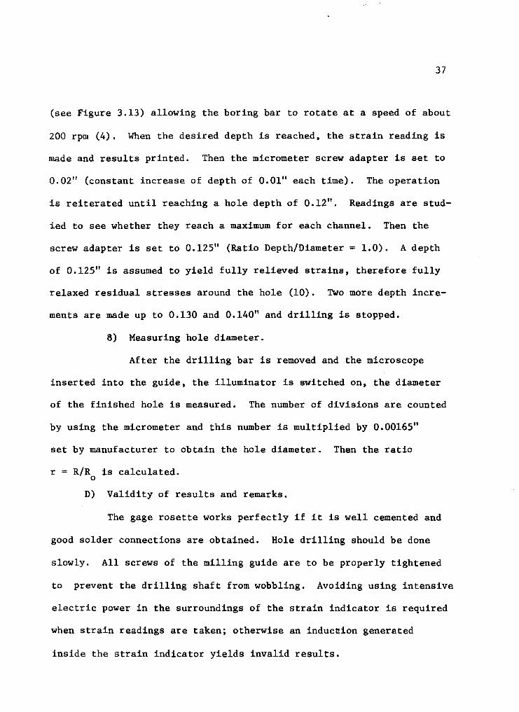
8) Drilling

The strain reading is set to zero for all three channels.

An electric drill is adapted to the milling bar by means of a universal

joint. A micrometer screw adapter (see Figures 3.11 and 3.12) is set

to zero but can allow several increments of hole depth totalling 0.125".

Now the screw adapter is set to 0.01" to permit a drill of 0.01" deep

hole. The trigger of the drill is squeezed moderately to operate it

SH

Figure 3.10 Adjustable swivel feet

figure 3.11 Mi lling bar (with drill bit and micrometer screw adapter)

35

36

SE' •

Figure 3.12 Drilling set up

Figure 3.13 Drilling under action

37

(see Figure 3.13) allowing the boring bar to rotate at a speed of about

200 rpm (4). When the desired depth is reached, the strain reading is

made and results printed. Then the micrometer screw adapter is set to

0.02" (constant increase of depth of 0.01" each time). The operation

is reiterated until reaching a hole depth of 0.12". Readings are stud-

ied to see whether they reach a maximum for each channel. Then the

screw adapter is set to 0.125" (Ratio Depth/Diameter= 1.0). A depth

of 0.125" is assumed to yield fully relieved strains, therefore fully

relaxed residual stresses around the hole (10). Two more depth incre­

ments are made up to 0.130 and 0.140" and drilling is stopped.

8) Measuring hole diameter.

After the drilling bar is removed and the microscope

inserted into the guide, the illuminator is switched on, the diameter

of the finished hole is measured. The number of divisions are counted

by using the micrometer and this number is multiplied by 0.00165"

set by manufacturer to obtain the hole diameter. Then the ratio

r = R/R is calculated. 0

D) Validity of results and remarks.

The gage rosette works perfectly if it is well cemented and

good solder connections are obtained. Hole drilling should be done

slowly. All screws of the milling guide are to be properly tightened

to prevent the drilling shaft from wobbling. Avoiding using intensive

electric power in the surroundings of the strain indicator is required

when strain readings are taken; otherwise an induc~ion generated

inside the strain indicator yields invalid results.

:·.- ..

38

3.1.2 Drilling inside holes.

side hole drilling procedure.

Inside hole drilling is similar to out­

Figures 3.14-3.17 show the test details.

3.1.3 Experiment of tensioning a steel plate specimen for the de­

termination of calibration coefficients. This experiment provides

information to calculate calibration coefficients under a controlled

condition for use in data adjustment of the results obtained from

the hole-drilling technique applied to the tube.

The experiment consists of tensioning a steel plate with an

initial force of known magnitude and measuring strains by means of a

rosette and a reference gage, before and after drilling a hole in the

plate. Then, the strains measured are analyzed to separate strains

due to applied stresses from strains due to unknown residual stresses

in the test plate. In this analysis, the effects of residual stresses

are eliminated, and the calibration coefficients are determined by the

strain-relaxation due to drilling method or by the method of separation

of induced stresses and applied stresses.

A) Material and gages.

T~e test pi~ce is ·a steel plate 5/16" thick having the shape

shown in Figure 3.18.

Three gages - rosette 125RE, position A (to measure initial

residual stresses) rosette 125RE, position B (to measure strain-relaxa­

tion due to drilling) and reference gage 250BG120 - is cemented to the

test piece (see Figure 3.18).

The reference gage belongs to a general purpose family of

constantant strain gages widely used in experimental stress analysis.

39

Figure 3.14 Set up for drilling inside hole

Figure 3.15 Cementing swivel feet

40

Figure 3.16 Alignment set up before drilling (inside surface)

41

Figure 3 .17 Inside hole drilling under action

• "' • (""\

•

J.5" J.s•

::::::r ---:J Reference gage

26• 12•

co<> ()

Rosette B

cot) ()

Rosette A

7•

Figure J.18 .:ilape or the steel plate specimen and position of gages (Rosettes A. and B and reference-gage)

• "' N -• "'

~ N

Its characteristics are:

Gage type: EA-06-250 BG -120

Resistance in ohms: 120.0 ± .15%

Gage factor at 75°F: 2.06 ± 0.5%

Option: L

Temperature range" -100°F to +350°F

Strain limits: 5% for gage lengths 1/8" and larger.

Cements: compatible with M-M 200 Catalyst and M-Bond 200 Adhesive

or M-Bond 610.

B) Apparatus.

43

The apparatus used to apply a series of tensions to the test

plate is a Material Testing System (MTS) with a load cell of 50 metric

ton capacity, Model 661-23A-02, serial number 152. (See Figures

3.19 and 3.20.) The strains relieved from the operation of tensioning

the test piece as well as of hole drilling (holes A and B) will be

measured by a strain indicator (see Figures 3.4 and 3.5).

C) Experimental set up.

1) Experiment of checking the existence of residual stresses

in the steel pipe.

The test plate cut to dimensions as shown in Figure 3.18

is put on a flat table. After installation of gage A on the plate

(see Figure 3.21) set to zero the strain indicator.

No load is applied during this experiment.

Attach the milling guide and drill hole with increment

of 0.01" hole depth each time up to total depth of 0.125" and record

results (see Figure 3.22).

44

SE~

Figure 3.19 Material Testing System (MTS)

SE~

Figure 3.20 Material Testing System with load cell

45 SIP

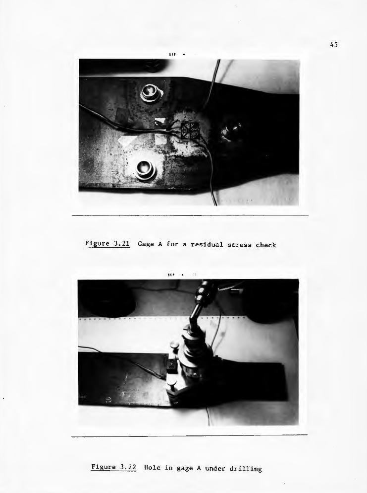
Figure 3.21 Gage A for a residual stress check

SI p

Figure 3.22 Hole in gage A under drilling

•

46

The results of this experiment indicated a residual stress

in the order of magnitude of 1000 psi. It will be seen later that the

effect of this stress is eliminated in the determination of calibration

coefficients.

2) Experiment of measuring the modulus of elasticity of the

test plate steel.

Apply tensions cr1

and cr2

to the plate and record from

the reference gage the corresponding strains El and E2

•

The modulus of elasticity E will be given by:

The computations done in paragraph 3.2.2 show E = 29*

6 10 psi.

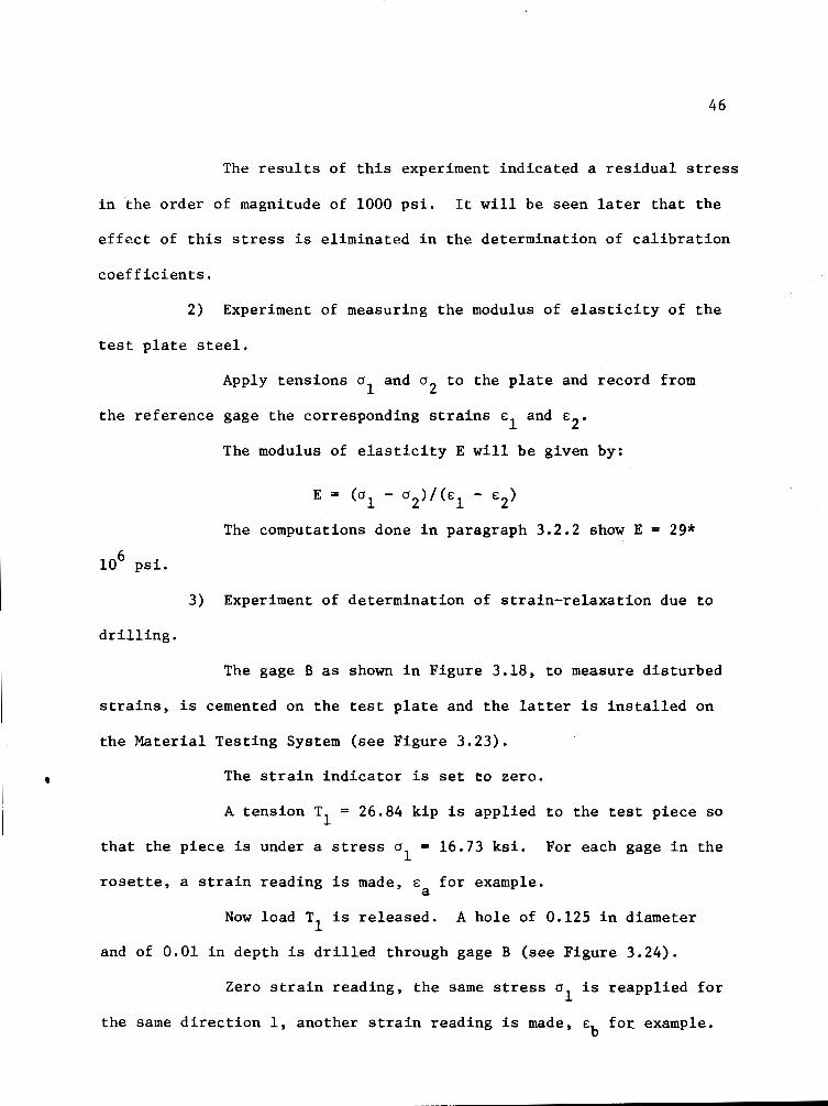
3) Experiment of determination of strain-relaxation due to

drilling.

The gage B as shown in Figure 3.18, to measure disturbed

strains, is cemented on the test plate and the latter is installed on

the Material Testing System (see Figure 3.23).

The strain indicator is set ~o zero .

A tension T1

= 26.84 kip is applied to the test piece so

that the piece is under a stress cr1

= 16.73 ksi. For each gage in the

rosette, a strain reading is made, E for example. a

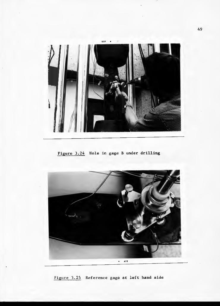
Now load T1 is released. A hole of 0.125 in diameter

and of 0.01 in depth is drilled through gage B (see Figure 3.24).

Zero strain reading, the same stress cr1

is reapplied for

the same direction 1, another strain reading is made, Eb for example.

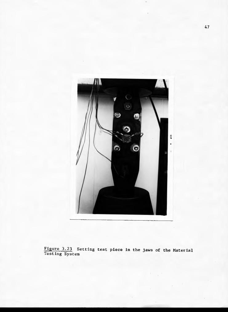
Figure 3.23 Setting test piece in the jaws of the Material Testing System

47

48

Compute 6€ = € € This difference between two read-a - b'

ings before and after drilling, with the same load applied to the

plate, represents the strain-relaxation due to drilling pertaining to

a hole depth of 0.01 inch, for the direction 1.

The cycle of operations is reiterated until the total

hole depth of 0.125 inch is reached.

The diameter of the hole is measured and checked with

the expected value of 0.125 inch.

At the end of one cycle of operations, readings are made

and recorded for other directions (gages) 2,3 and for the reference

gage for an eventual comparison. (See Figure 3.25.)

Finally for a total hole depth of 0.125 inch is reached,

~El Eal - Ebl = strain relaxation due to drilling for direction 1

strain relaxation due to drilling for direction 2

~€3 = Ea3 - Eb 3 = strain-relaxation due to drilling for direction 3.

These three relaxed strains ~€ 1 , ~€ 2 , ~€ 3 are treated as regular

measured strains to provide calibration coefficients. The testing

procedure has eliminated any effect of initial residual stresses.

Results will be shown in the paragraph 3.2.2 "Test results".

4) Experiment of separation of induced stresses and applied

stresses.

The gage B as shown in Figure 3.18 is cemented on the plate

which is mounted on the Material Testing System.

The strain indicator is set to zero. A tension T1

49

s Er

Figure 3.24 Hole in gage B under drilling

4lS

Figure 3.25 Reference gage at left hand side

50

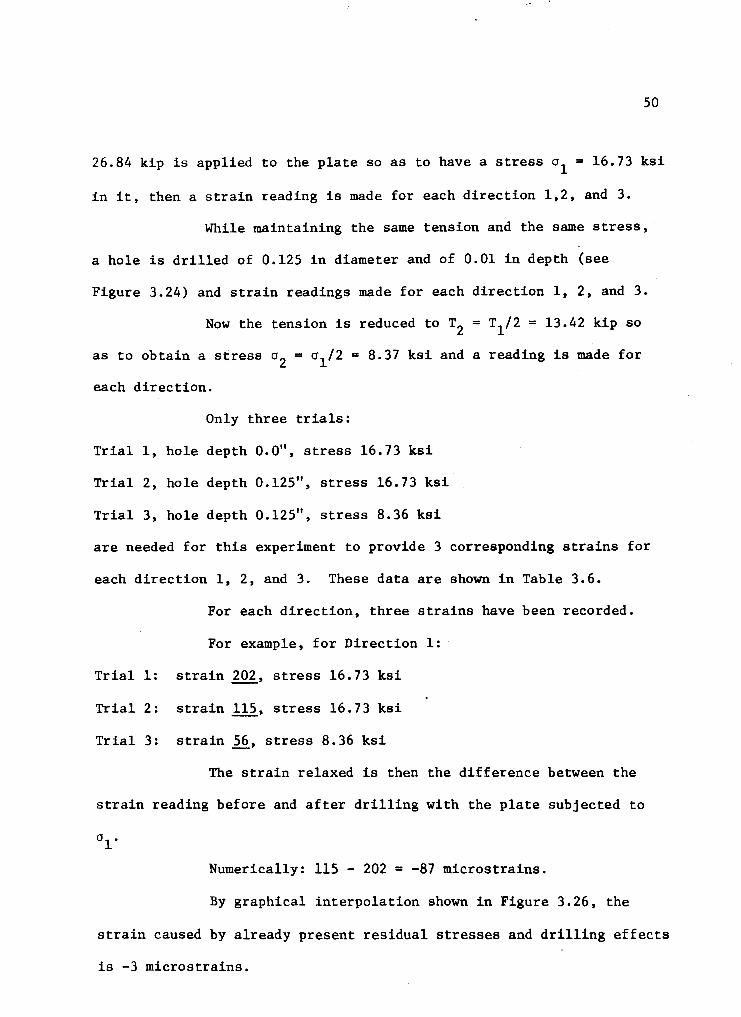
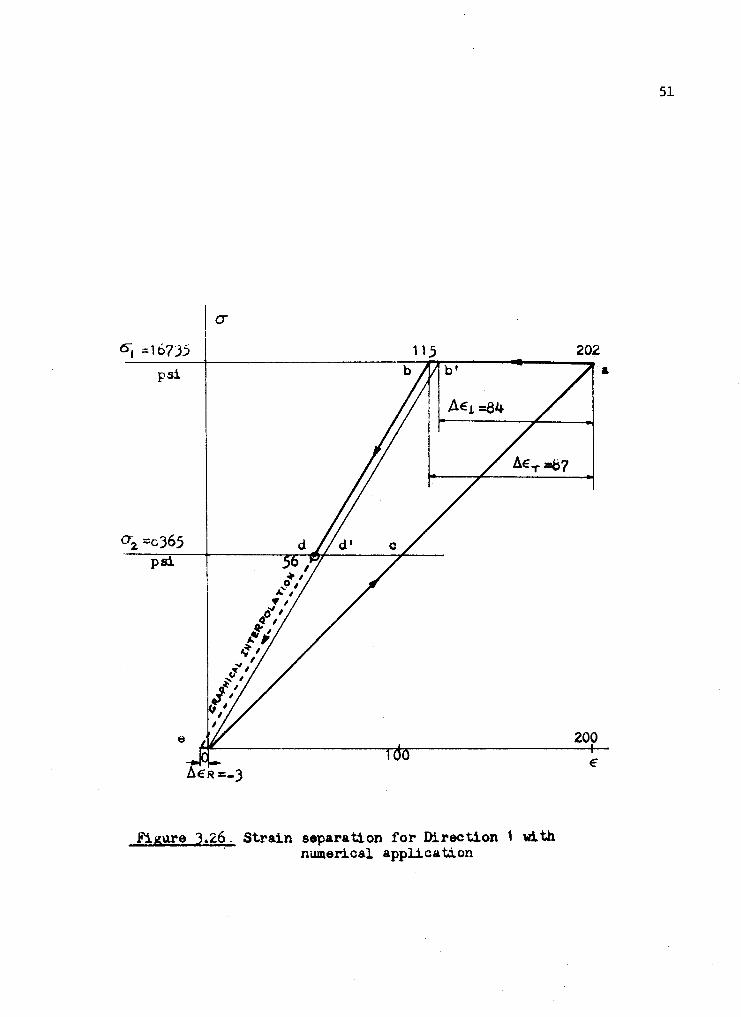
26.84 kip is applied to the plate so as to have a stress a1 = 16.73 ksi

in it, then a strain reading is made for each direction 1,2, and 3.

While maintaining the same tension and the same stress,

a hole is drilled of 0.125 in diameter and of 0.01 in depth (see

Figure 3.24) and strain readings made for each direction 1, 2, and 3.

Now the tension is reduced to T2 = T1/2 = 13.42 kip so

as to obtain a stress a2 = a1/2 = 8.37 ksi and a reading is made for

each direction.

Only three trials:

Trial 1, hole depth O.O", stress 16.73 ksi

Trial 2, hole depth 0.125", stress 16.73 ksi

Trial 3, hole depth 0.125", stress 8.36 ksi

are needed for this experiment to provide 3 corresponding strains for

each direction 1, 2, and 3. These data are shown in Table 3.6.

For each direction, three strains have been recorded.

For example, for Direction 1:

Trial 1: strain 202, stress 16.73 ksi

Trial 2: strain 115, stress 16.73 ksi

Trial 3: strain 56, stress 8.36 ksi

The strain relaxed is then the difference between the

strain reading before and after drilling with the plate subjected to

al.

Numerically: 115 - 202 = -87 microstrains.

By graphical interpolation shown in Figure 3.26, the

strain caused by already present residual stresses and drilling effects

is -3 microstrains.

CT

6j =167)5 115

psi

AE1 ::84

0-2 =cJ65 psi

e

f1ER =-J

Figure ).2.6. Strain separation for Direction 1 w1 th numerical application

51

202 a

200

E

Strain due to applied stress 6£1 = -87-(-3) = -84

By the same approach, it has been found:

6£ = -143 2

6£ = -25 3

These strains due to applied stresses are treated as

measured strains:

s = 6£ + 6£ = -84 - 25 = -109 1 3

D = 6£ - 6£ = -84-(-25) = -59 1 3

Tan 28 = (S - 26£2)/D ~ (-109-2(-143))/-59 • -177/59

Cos 28 • 0.316227

From equations (3a), Appendix III:

4A = 2S/(a1 + a 2)

4B = 2D/((a1 - a 2) Cos 28)

The experiment has provided:

a1 = 16730 psi, a2

= 0

Finally:

4A = 2(-109)10-6/16730 = -1.30(10-8)

4B = 2(-59)10-6/(16730 * 0.316227) • -2.23(10-8)

3.2 TEST RESULTS

3.2.1 Results from the hole drilling experiments on the steel tube.

52

Results from the experiments of hole drilling from the outside

surface of the tube for Hole #1 are shown in detail in Tables 3.1 and

3.2. These tables give for 13 trial hole depths, measured strains for

gages a,b,c, principal stresses a1 and a2

for each set of strains in

three directions, longitudinal stresses a1 and circumferential stresses

53

TABLE 3.1

EXPERIMENT OF OUTSIDE HOLE DRILLING

RESULTS FOR HOLE 1

Trial Hole Measured strains

------------------------------------------II Depth Gage a Gage b Gage c

1 0.01" 2 10 8

2 0.02 3 14 14

3 0.03 5 22 25

4 0.04 4 24 39

5 0.05 7 - 31 49

6 0.06 7 30 55

7 0.07 6 30 62

8 0.08 6 30 67

9 0.09 5 27 70

10 0.10 2 26 72

11 0.11 3 30 73

12 0.125 4 27 75

13 0.13 I 3 26 72 I

54

TABLE 3. 2

(Continued)

Trial Hole I 01 02 OL OT crL x fl Depth psi psi psi psi y

1 0.01" -1190 -1799 -1744 -1214 -0.04 -

2 0.02 -1332 -2576 -2394 -1514 -0.06

3 0.03 -2472 -4425 -4008 -2888 -0.09

4 0.04 -3528 -6357 -5143 -4743 -0.12

5 0.05 -4730 -8134 -6677 -6197 -0.16

6 0.06 -5205 -9048 -7206 -7046 -0.18

7 I 0.07 -5554 -10079 -8136 -7496 -0.20

8 0.08 -5896 -10885 -8911 -7871 -0.22

9 0.09 -5880 -11353 -9461 -7781 -0.23

10 0.10 -5571 -11411 -9386 -7626 -0.23

11 0.11 -5863 -11600 -9376 -8096 -0.23

12 0.125 -6200 -11920 -10080 -8080 -0.24

13 0.13 -5711 -11530 -9541 -7701 -0.23

55

OT' ratio of oL to yield stress oy.

As the quantity of data is great, it has been simplified and

shown in Table 3.3 . Only data relating to depth 0.125 inch is shown,

comprising strains in three directions, values of data reduction co-

efficients 4A and 4B, principal stresses o1

and o2 , longitudinal,

circumferential stresses and ratio of o1 to yield stress oy.

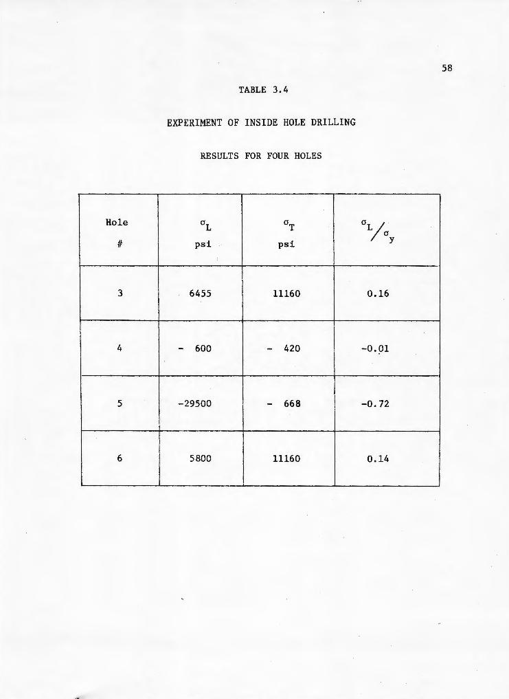
In Table 3.4 are shown results pertaining to inside holes com-

prising longitudinal, circumferential stresses, ratio of a1 to yield

stress o for hole depth of 0.125 inch. y

In light of the data shown in these tables, an evaluation of

results can be made, leading to some pertinent remarks and proving

that the stress field in the welded fabricated steel tube is uniform.

A) Remarks.

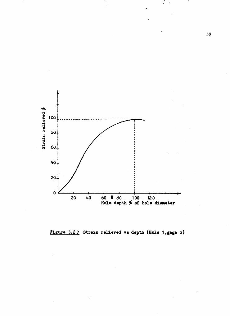
A survey of values of strains for each gage in Table 3.2

shows that they gradually increase with hole depth, reach a peak

for a 0.125 inch depth then slightly decrease (see Figure 3.27).

This fact confirms the assertion by Bush and Kromer (2) and by S.

Redner (10) that the strains relieved attain a limiting value and a

maximum when hole depth approaches the hole diameter.

A second remark is that the values of stresses computed from

strains measured by three gages a,b,c for one hole ~ gradually increase

and reach a maximum for ratio depth to hole radius equal to 1.0 and

slightly decrease further.

Finally, values of longitudinal residual stresses found

from outside and inside holes agree. In fact, for four holes number

3,4,5 and 6, the ratio of o1 to oy for outside and inside holes are

56

TABLE 3.3

EXPERIMENT OF OUTSIDE HOLE DRILLING

DATA AND RESULTS FOR 11 HOLES

(HOLE DEPTH 0.125")

Hole Micro-strains 4A • 4B •

II ---------- --------- ----------- (*10-8) (*10-8) E: E:b E: a c

1 40 27 75 -0.87 -2.50

2 -41 -25 -77 -0.88 -2.50

3 -24 -36 -41 -0.88 -2.50

4 -51 15 18 -1.05 -2.68

5 149 30 59 -0.85 -2.45

6 -31 -18 -32 -0.88 -2.50

7 -32 -90 -102 -0.85 -2.45

8 -35 -17 -21 -0.85 -2.45

9 -89 79 -104 -0.95 -2.60

A 97 101 29 -0.83 -2.37

B 20 12 92 -0.83 -2.37

* These values of 4A and 4B based on Figure 2.J

57

TABLE 3.3

(Continued)

Hole cr 1 cr 2 crL crT crL

/a It psi psi psi · psi y

1 -6070 -12091 -10080 -8080 -0.24

2 10331 16487 16090 16130 0.24

3 6651 8122 7106 7666 0.17

4 6629 -343 792 5494 0.02

5 -31541 -17401 -30510 -18430 -0.75

6 6078 8240 6079 8239 0.13

7 12346 19184 13890 17640 0.34

8 7652 5524 5690 7486 0.14

9 6803 33828 33820 6816 0.80

A -19484 -10878 -18390 -11970 -0.45

B -8696 - -18292 -17210 -9781 -0.42

58

TABLE 3.4

EXPERIMENT OF INSIDE HOLE DRILLING

RESULTS FOR FOUR HOLES

Hole aL OT oL/oy

II psi psi

3 6455 11160 0.16

4 - 600 - 420 -0.01

5 -29500 - 668 -0. 72

6 5800 11160 0.14

59

~

-·------------------- - --- ----~ ' ~ : 100

CD

~ J.o bO '" ~ t; 60

40

20

a : ' ' '

20 40 60 • 80 100 120 Hole depth ~ ot hole diaaeter

Figura 3.2 Z Strain relieved vs depth (Hole 1 .&&I• c)

respectively:

0.17 and 0.16 (deviation 0.01 of cr ) y

0.02 and -0.01 (deviation 0.03 of a ) y

-0.75 and -0.73 (deviation 0.02 of a) y

0.13 and 0.14 (deviation 0.01 of a ) y

60

These deviations appear low and suggest a well behaved stress

distribution.

B) The substantiation of the uniform field of residual stresses

in the tube is now presented.

According to Kelsey (1), in a uniform field of stresses,

the relationship between surf ace strain and hole depth is proportional

to the magnitude of the stress. In other words, the incremental change

in surface strain ~Ezi' for an incremental change in hole depth ~zi

is proportional to the magnitude of the stress crzi·

For a material following Hooke's law

E = cr/E

but for the hole drilling method, the incremental strain is not a

direct measure of the average residual stress in a given increment of

hole depth. Therefore, a factor of proportionality K must be intro-

duced:

~E i = Ka ./E Z Z1

Equations for the strains corresponding to the stresses in

two perpendicular directions are:

EL = crL/E

ET = crT/E

µcrT/E

µo1

/E

(1)

(2)

61

In the hole drilling method, the above equations become:

6£L = KlcrL/E - µK2 crT/E (3)

6£T = KloT/E - µK2 crL/E (4)

Solving (3) and (4) in terms of L and T gives:

2 2 2 crL = E/(Kl - µ K2) (~ (6£L) + µK2 (6£T)) (5)

2 2 2 crT = E/(Kl - µ K2) (K1 (6ET) + K2 (6£L)) (6)

Now solving equations (3) and (4) for the factors of pro-

portionality gives:

2 2 K1 = E/(crL - crT)(crL(6eL) - oT(6eT))

2 2 K2 = E/µ(oT - oL)(oL(6£T) - oT(6eL))

Using the steel plate data,

OL = 16 730 psi a = 0 T

µ = 0.29 E = 29(106)

-6 EL = 195(10 ) -6 £T = 40(10 )

and using equations (7) and (8) to compute K1 and K2 for the test

plate:

For the hole depth from 0.0 to 0.025",

K _ 29 (106) ( -6 1 - (16730)2 - O 16730 (195)(10 ) - O) • 0.338

- 29 (106) -6 . K2 - n ~n fn 1£~~n?, (16730 (40)(10 ) - O) • -0.239

(7)

(8) -

The computed values of K1 and K2 for dif~erent hole depths

varying from 0 to 0.125", are summarized in Table 3.5.

: '•

62

TABLE 3.5

VALUES OF FACTORS OF PROPORTIONALITY K1 AND K2 FOR THE PLATE

Hole depth Kl K2

o.o -0.025" 0.338 -0.239

0.025-0.050 0.324 -0.236

0.050-0.075 0.310 -0.281

0.075-0.100 0.296 -0.304

0.100-0.125 0.286 -0.329

Kelsey (1) has shown in his Table I for his first series of tests

relating to a uniform stress field, that .when his plate is subject to

a tension T1

(causing a uniform stress o1

in his plate) and subject

later to a tension T2 (causing a uniform stress o2) the_ respective

longitudinal and transverse strains £Ll' £Tl and £L2 £T2 are bound

by the relationships:

£Ll = £L2

£Tl = £T2

01

02 (= 2.0 for his case)

A first sample of calculation to prove the equality of the above

ratios is taken from a study by Kelsey (1, Table I):

For the depth of 0.250" of a hole drilled in a uniform stress

field:

£Ll = -376 microstrains, £Tl = 122 microstrains, oLl = 9700 psi

£L2 = -800 £T2 = 249 OL2 = 19400 psi

Ratios:

EL2

ELl 2.1,

ET2

ETl 2.0,

aL2 2.0 --- =

crLl

A second sample of calculation to substantiate the equality of

these ratios is taken from the case of our steel plate subject to

uniform tensions r1 and r 2 , data read from the Hole B with a hole

depth of 0.125":

ELl = 82 microstrains, ETl = 27 microstrains, crLl = 8370 psi

EL2 = 165 e:T2 = 55 <JLZ = 16730 psi

Ratios:

e:Ll 2.0, tT2 =

e:Tl 2.0, aL2 = e:L2 =

crLl 2.0

The ~alues of these ratios of strains and stresses show good

agreement.

To prove that a non-uniform stress field does not have these

characteristics: that is =

e:L2 e:T2 °L2 -.;-1-e:Ll e:Tl oLl

reference is again made to Kelsey, Table II (1) for a non-uniform

e:L2 e:T2 stress field studied by Kelsey shows that the ratios~. -, ~-,

e:Ll e:Tl 0:L2

crLl are not equal (see Table 3.6).

63

64

TABLE 3.6

DATA FROM A NON-UNIFORM STRESS FIELD

Hole ~(i+l) e:T(i+l~ PL

0L(i+l~ crL

0L{i+l~ depth £1

~i e:T

e:Ti 0 Li 0 Li (a) (b)

0.025" -122 20 18600 18700

2.24 -- 2.0 0.89 0.88

0.050 -274 40 16600 16500

1.50 1.47 0.88 0.92

0.075 -411 59 14600 15200

1.21 1.27 0.86 0.92

0.100 -498 75 12600 14000

1.10 -- 1.21 0.84 0.87

0.125 I -548 91 10600 12200

1.06 1.13 0.81 1.21

0.150 -583 103 8600 14800 i

1.04 1.09 o. 76 1.21

0.175 -607 I

112 6600 17900

(a) Values computed directly from measured strains

(b) Values calculated using K1 and K2 from a uniform stress field.

In order to substant i a t e that the field of residual stresses

present in the steel tube i s uniform, through the depth, we first

calculate the stresses cr1 i and crL(i+l) corresponding to hole depths

65

Zi and Zi+l in the steel tube, using K1 and K2 obtained from the test

plate and the corresponding hole depths in the test plate.

e:L(i+l) e:T(i+l) The second step is to compute the ratios

e:Li e:Ti

crL(i+l) and compare. crLi

Sample calculation:

and

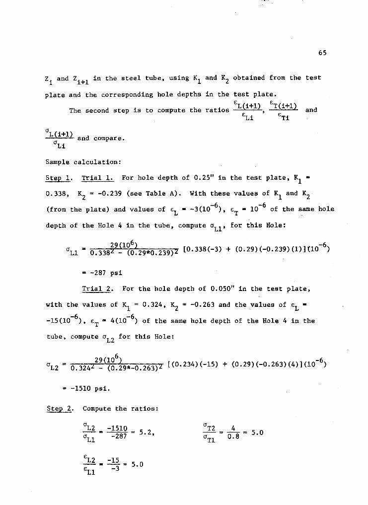
Step 1. Trial 1. For hole depth of 0.25" in the test plate, K1 =

0.338, K2

= -0.239 (see Table A). With these values of K1 and K2 -6 -6 (from the plate) and values of e:L = -3(10 ), e:T • 10 of the same hole

depth of the Hole 4 in the tube, compute crLl' for this Hole:

crLl 6 -6 = 29(10) [0.338(-3) + (0.29)(-0.239)(1))(10 )

= -287 psi

Trial 2. For the hole depth of 0.050" in the test plate,

with the values of K1

= 0.324, K2 = -0.263 and the values of e:L =

-6 -6 -15(10 ), e:T = 4(10 ) of the same hole depth of the Hole 4 in the

tube, compute crL2 for this Hole:

crL2 - 29(106) . - 0.3242 - (0.29*-0.263)2 [(0.234)(-15) + (0.29)(-0.263)(4)](10-

6)

= -1510 psi.

Step__l_. Compute the ratios:

0 L2 -1510 --= -287 =

5 · 2 • 0 Ll

(J T2 4

(J = -Tl 0.8 = 5.0

e: L2 = -15 = 5 .0

e:Ll - 3

The deviation: (5.2-5.0)/5.0 = 0.04 of £L2/£Ll appears

acceptable.

The computations of crL and crT and the required ratios are

summarized in Table 3.7. E

The ratios of L(i+l) ~i

ET(i+l)

£Ti

crL(i+l) 0 Li

show close

agreement, and the uniform stress field assumed in Chapter II is

substantiated by numerical calculation.

3.2.2 Tensioning and calibration experiment.

A) Results of the test.

Data derived from the experiment of strain-relaxation due

to drilling are condensed in Table 3.8. These data will be used in

section 3.2.2.c to compute the values of calibration coefficients

4A and 4B.

Data pertaining to the experiment of separation of induced

stresses and applied stresses are shown in Table 3.9. Calibration

coefficients 4A and 4B are computed from these data and described in

section 3.2.2.d.

B) Computation of the value of modulus of elasticity.

66

The modulus of elasticity in a strain-stress curve is given

by the slope of the straight part of the curve. As the maximum stress

applied to the plate is 0.40 F (within the limit of elasticity) Hooke's y

law is valid and:

E = a/£ or E = (o2 - crl)/(£2 - £1)

A measurement of the thickness and width of the plate pro-

vides:

I Trial Hole I depth

1 .025"

2 .050

3 .075

4 .100

5 .125

TABLE 3.7

RESULTS OF APPLICATION TO TUBE DATA. (HOLE 4)

e:L e:T crL crT e:L(i+l 0 L(i+l2 (µ strain) (µ strain) p~i psi e:L (i) 0 L(i)

-3 0.8 -287 145

5.0 5.2

- 5 4 -1510 714

1.6 1. 7

-24 6 '-2570 1237

1.1 1.1

-26 7 -3019 1585

1.2 1.2

-30 9 -3765 2151 '

e:T(i+l2

e:T(i)

5.0

1.5

1.2

1.3

0 T(i+l) 0 T(i)

4.9

1. 7

1.2

1.3

°' .......

.:

68

TABLE 3.8

EXPERIMENT OF TENSIONING & CALIBRATION

DATA FROM STRAIN-RELAXATION METHOD

Trial Hole Hole Measured Reference Stress micro-

If Depth Diame- strains gauge Applied ter ---------------- (ks·i)

£1 £2 £3

1 o.o 0.0 202 533 193 572 16.73

2 .025 .20 197 515 185 572 16.73

3 .050 .40 182 474 171 572 16.73

4 .075 .60 171 442 161 572 16.73

5 .100 .80 165 423 156 570 16.73

6 .125 1.00 162 407 155 571 16.73

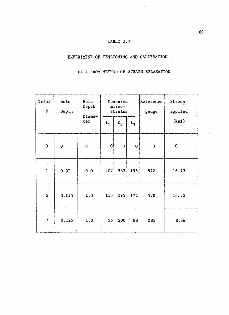
69

TABLE 3.9

EXPERIMENT OF TENSIONING AND CALIBRATION

DATA FROM METHOD OF STRAIN RELAXATION

Trial Hole Hole Measured Reference Stress ·-Depth mirco-

II Depth strains gauge applied Diame- -------------ter e:l e:2 e:3 (ksi)

0 0 0 0 0 0 0 0

1 0.011 0.0 202 533 193 572 16.73

6 0.125 1. 0 ll5 395 172 570 16. 73

7 0.125 1.0 56 200 88 285 8.36

70

Thickness: 5/16" or 0.3125"

Width: 5 1/8" or 5.125"

True cross-sectional area: 1.60 square inches

As applied tensions were 26.8 kip and 13.4 kip and

parallel to longitudinal axis, relative stresses would be respectively:

OLZ = 26.8/1.6 ~ 16.73 ksi

OLl = 13.4/1.6 = 8.37 ksi

The corresponding strains measured we~e:

£L2

• 574 microstrains

£Ll • 286 microstrains

Finally:

Ea (16.73 - 8.37)103/(574-286)10-6

6 • 29 x 10 psi

C) Results from method of strain-relaxation due to drilling.

From Table 3.5, the strain-relaxation due to drilling (2)

equals the difference of strain readings before and after drilling

(depth 0.125") when the test plate is under the same applied load

(16.73 ksi):

For direction 1:

= -202 + 162 = -40 microstrains

For direction 2:

= -533 + 407 -126 microstrains

For direction 3:

• -193 + 155 = -38 microstrains

These strains of strain-relaxation due to drilling are

treated as measured strains (see equations (3a), Appendix III):

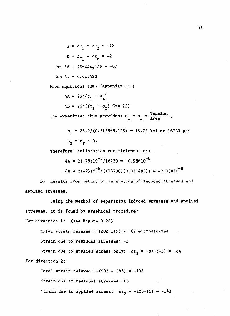
S = ~E + ~E = -78 1 3

D = ~£ - ~£ = -2 1 e

Tan 2e = (S-2~E )/D = -87 2

Cos 2e = 0.011493

From equations (3a) (Appendix III)

4A = 2S/(a1 + a2)

4B = 2S/((a1 - a2) Cos 2e)

The experiment thus provides: a = 0 = Tension 1 L Area

a1

= 26.9/(0.3125*5.125) = 16.73 ksi or 16730 psi

a2 = aT = 0.

Therefore, calibration coefficients are:

4A = 2(-78)10-6/16730 = -0.~'*10-8

4B = 2(-2)10-6/((16730)(0.011493)) = -2.08*10-8

D) Results from method of separation of induced stresses and

applied stresses.

Using the method of separating induced stresses and applied

stresses, it is found by graphical procedure:

For direction 1: (see Figure 3.26)

Total strain relaxes: -(202-115) = -87 microstrains

Strain due to residual stresses: -3

Strain due to applied stress only: 6E1 = -87-(-3) • -84

For direction 2:

Total strain relaxed: -(533 - 395) = -138

Strain due to residual stresses: +5

Strain due to applied stress: 6c = -138-(5) = -143 2

71

For direction 3:

Total strain relaxed: -(193-172) = - 1

Strain due to residual stresses: +4

Strain due to applied stress: 6e3 = -21-(4) = -25

These strains due to applied stresses are treated as

measured strains:

S = 6E + 6E = -109 1 3

D = 6E - 6E - -59 1 3

Tan 28 = (S - 26£2)/D a -177/59

Cos 2a = 0.316227

From equations (3a)

4A = 2S/(o1 + o2)

4B = 2D/((o1 - o2) Cos 2S)

It has been found by experiment that:

cr1 = 16730 psi, 02 .. 0

Therefore:

4A = 2(-109)10-6/16730 • -1.30*10-8

4B = 2(59)10-6/(16730*0.316227) = -2.23*10-8

E) Summary of results.

In this investigation, four ways of ·computing the values

of 4A and 4B were used.

1) For each hole drilled, its radius R is measured and 0

the ratio r of the distance of the gage to center R(R•0.202" for

Rosette 125RE) to radius of hole drilled R (r•R/R ) is evaluated. 0 0

In Figure 2.3 the line of abscissa r parallel to vertical axis,

cuts the curve 4A at point a and the curve 4B at point b, the

72

73

ordinates of a and b are the values of 4A and 4B. The values of

4A and 4B of the 11 drilled holes are sununarized in Table 3.10.

It is of interest to note that in Table 3.10 4A and 4B

differ for different holes, because they are determined from equations

which are functions of r, r=R/R , r varies with R where R is the 0 0 0

measured radius of the hole drilled.

TABLE 3.10

VALUES OF 4A AND 4B COMPUTED BY CURVES FROM FIGURE 2.3

4A 4B Hole (10-8) (10-8)

1 -0.87 -2.50

2 -0.87 -2.50

3 -0.85 -2.45

4 -1.05 -2.48

5 -0.85 -2.45

6 -0.88 -2.50

7 -0.85 -2.45

8 -0.85 -2.45

9 -0.95 -2.60

A -0.83 -2.37

B -0.83 -2.37

2) From equation (1)

l+µ 2 4 Er = -o1 ZE [1/r - 3/r (Cos 2a) + 4/(1+µ) (Cos 2a)

and

Er = (A + B Cos 2a)o1

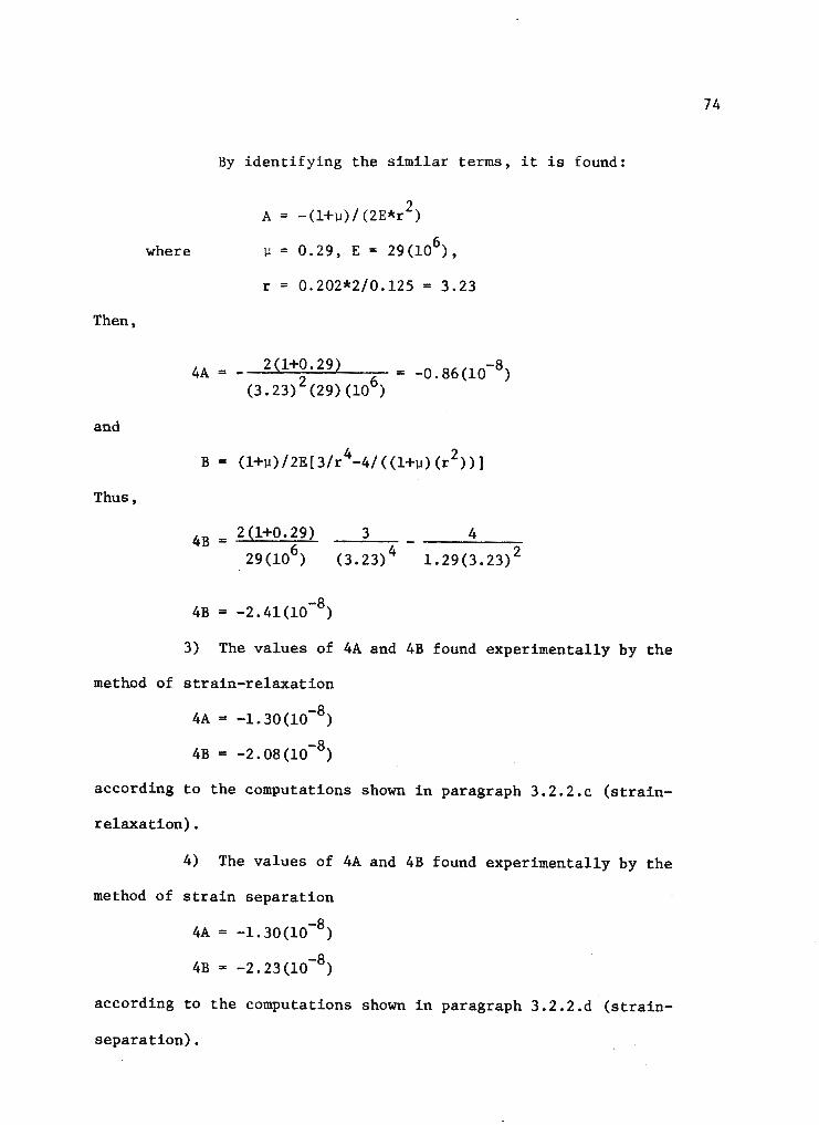
Then,

and

Thus,

where

By identifying the similar terms, it is found:

A=

µ =

2 -(l+µ)/(2E*r )

6 0.29, E = 29(10 ),

r = 0.202*2/0.125 = 3.23

4A = 2 Cl+0.29) (3.23) 2 (29)(106) = -0.86(10-8)

Ba (l+µ)/2E[3/r 4-4/((l+µ)(r 2))]

4B = 2(1+0.29)

29 (106)

4B = -2.41(10-8)

3

(3.23) 4 4

1.29(3.23) 2

3) The values of 4A and 4B found experimentally by the

method of strain-relaxation

4A = -1.30(10-8)

4B = -2.08(10-8)

according to the computations shown in paragraph 3.2.2.c (strain-

relaxation).

4) The values of 4A and 4B found experimentally by the

method of strain separation

4A = -1.30(10-8)

4B = -2.23(10-8)

according to the computations shown in paragraph 3.2.2.d (strain-

separation).

74

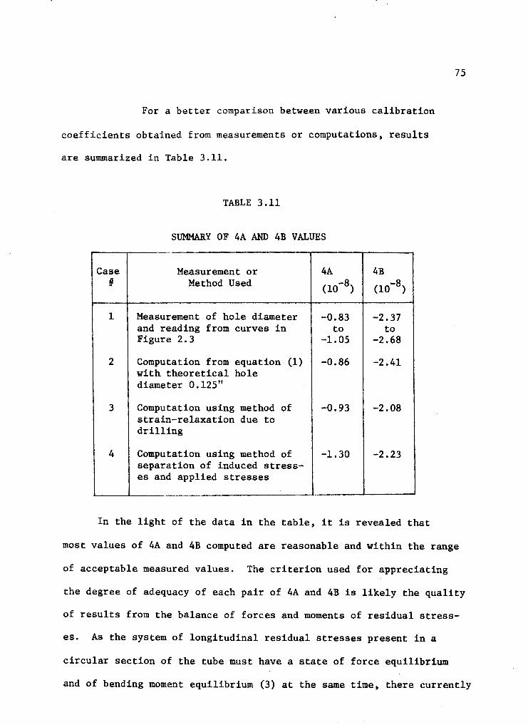
75

For a better comparison between various calibration

coefficients obtained from measurements or computations, results

are sununarized in Table 3.11.

TABLE 3.11

SUMMARY OF 4A AND 4B VALUES

Case Measurement or 4A 4B II Method Used (10-8) (10-8)

1 Measurement of hole diameter -0.83 -2.37 and reading from curves in to to Figure 2.3 -1.05 -2.68

2 Computation from equation (1) -0.86 -2.41 with theoretical hole diameter 0.125"

3 Computation using method of -0.93 -2.08 strain-relaxation due to drilling

4 Computation using method of -1.30 -2.23 separation of induced stress-es and applied stresses

In the light of the data in the table, it is revealed that

most values of 4A and 4B computed are reasonable and within the range

of acceptable measured values. The criterion used for appreciating

the degree of adequacy of each pair of 4A and 4B is likely the quality

of results from the balance of forces and moments of residual stress-

es. As the system of longitudinal residual stresses present in a

circular section of the tube must have a state of force equilibrium

and of bending moment equilibrium (3) at the same time, there currently

'· ·:·•··:.

is a deviation in the results given by the computation of balancing

forces and moments of residual stresses; this deviation derives from

accumulation of errors during experimentation. Because force and

moment balancing will be described in Chapter IV, it is appropriate

to evaluate the results of calibration coefficients after obtaining

results of balancing.

F) Application of calibration coefficients to tube data.

After obtaining all pairs of calibration coefficients 4A

and 4B for each case as shown in Table 3.7, it is necessary to apply

these coefficients to tube data and determine the corresponding

longitudinal residual stresses, circumferential residual stresses

and ratios of longitudinal residual stresses to yield stress, and to

plot curves of the distribution. Curves are built with d/R on the

abscissa (d = distance of hole to the weld, R c radius of the tube)

and oL/oy on the ordinate.

Case 1. Results relating to initial values of longitudinal and cir-

cumferential stresses derived from measured strains, are given in

Table 3.3. The relative calibration coefficients 4A and 4B are

obtained from the curves in Figure 2.3.

The corresponding curve of o1 /oy is drawn in Figure 3.28.

Case 2. Results pertaining to data reduction coefficients 4A and

4B computed from equation (1), are shown in Table 3.12.

The corresponding curve is drawn in- Figure 3.29.

Case 3. Results pertaining to calibration coefficients obtained

from method of strain-relaxation due to drilling, are condensed in

Table 3.13.

76

O.d

0.4

Ei~

6':s O.b

0.)4

0 "" " J.O x.

- 0.4

-0.75

Figure 3,28 Curve of initial values ot measured longitudinal residual stresses

d R

......

......

Hole

II

1

2

3

4

5

6

7

8

9

A

B

TABLE 3. 12

RESULTS WITH COMPUTED CALIBRATION COEFFICIENTS

4A = -0.86(10-8)

4B = -2.41(10-8)

01 OT

psi psi

-10220 - 8149

10900 16540

7268 7849

1223 6451

-30330 -18040

6205 8446

13670 17490

5599 7424

37010 7877

-18390 -11970

-16670 - 9372

78

01

/';; y

-0.25

0.27

0.18

0.03

-0.75

0.15

0.33 I

0.14 I 0.90

-0.45

-0.41

~ -6"~

0.90

o.o

0.4 O.JJ

OJ__.J_.~--~--~--~-,/.~--~-+-~~--~~-:---~_._~-+-~.._.-;:;-~-:;-'~---2.0 J.O Jt

- o.4

- o.8 f

Figure J.29 Curve or longitudinal residU&l. stresses recalculated vi th data red®tion coetticientai 4A • '.'"0.86(10-8) , 48 • -2.41(10-e)

d R.

" \0

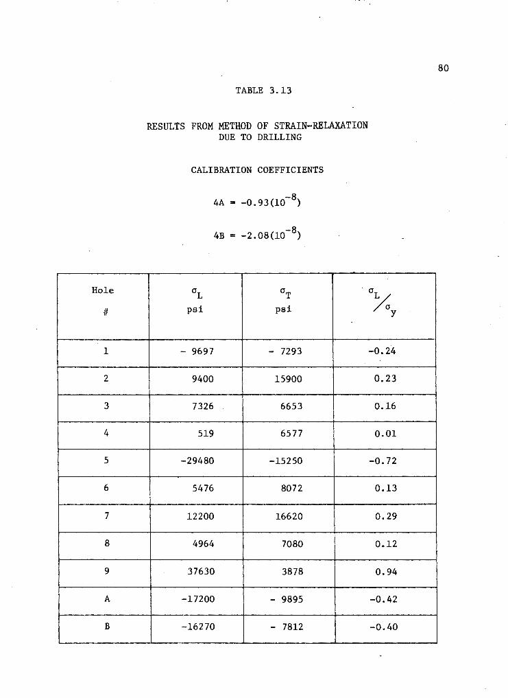
Hole

II

1

2

3

4

5

6

7

8

9

A

B

TABLE 3.13

RESULTS FROM METHOD OF STRAIN-RELAXATION DUE TO DRILLING

CALIBRATION COEFFICIENTS

4A = -0.93(10-8)

4B = -2.08(10-8)

aL OT - aL

/a psi psi y

- 9697 ,... 7293 -0.24

9400 15900 0.23

7326 6653 0.16

519 6577 0.01

-29480 -15250 -0. 72

5476 8072 0.13

12200 16620 0.29

4964 7080 0.12

37630 3878 0.94

-17200 - 9895 -0.42

-16270 - 7812 -0.40

80

The curve is shown in Figure 3.30.

Case 4. Results relating to calibration coefficients calculated

from method of separation of induced stresses and applied stresses,

are shown in Table 3.14.

The curve is given in Figure 3.31.

81

A preliminary survey of these curves shows that the one in case

4 is likely to lead to good results in balancing forces and moments

because of the reduced tension and a slight compressive area at

hole number 4 which helps in moment balancing.

o.c

o.4

6"1.

ff'~

0.9-.

0.29 -

0 l I I . • - 2.0 J.O Jt.

-0.

-0.8 -0-;72

Figure J.lQ Curve ot longitudinal residual. stresses computed troa strain-relaxation aethod w1 th calibration coefficients :4A=-0.9.3( 10-s ).4B=-2.08( 10-8 )

d R

(X) N

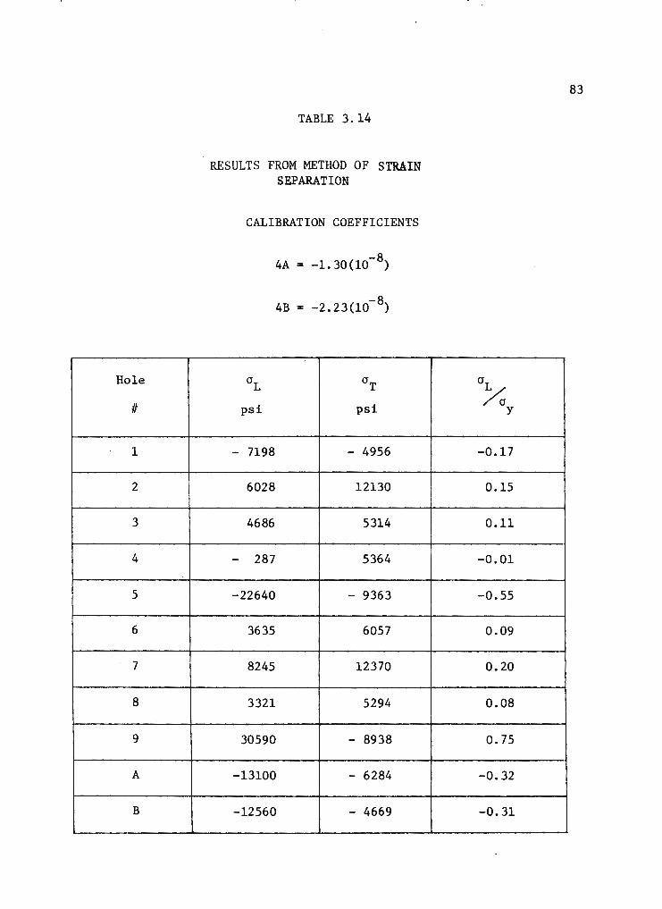
Hole

II

1

2

3

4

5

6

7

8

9

A

B

TABLE 3.14

RESULTS FROM METHOD OF STRAIN SEPARATION

CALIBRATION COEFFICIENTS

4A = -1. 30(10-8)

4B = -2.23(10-8)

OL OT

psi psi

- 7198 - 4956

6028 12130

4686 5314

- 287 5364

-22640 - 9363

3635 6057

8245 12370

3321 5294

30590 - 8938

-13100 - 6284

-12560 - 4669

83

OL /a y

-0.17

0.15

0.11

-0.01

-0.55

0.09

0.20

0.08

0.75

-0.32

-0.31

e:. 0.8

6':.

0.15

0.4

0

-0.4

-0.8

0.20

2.0

Figure J.31 Curve of longitudinal residul stresses computed troa method of strain separ•tiOll vi th calibration coe!!ioients: 4.A =-1.JO( 10-a)_, QB •-2.2J( 10-e).

J.O Jt. d. R.

co .s;,..

: .•..

CHAPTER IV

BALANCE OF FORCES AND MOMENTS

As a means of checking the correctness of results of the measure-

ment of residual stresses by the hole-drilling technique a balance

of forces and moments pertaining to longitudinal residual stresses is

in equilibrium in the steel tube, the summation of forces and moments

with respect to an axis must equal zero (3). It is convenient to show

the balancing of forces and moments, using calibration coefficien~s

obtained from theory and published literature and experimentally

determined.

4.1 BALANCING FORCES AND MOMENTS OF RESULTS USING ANALYTICALLY DERIVED CALIBRATION COEFFICIENTS

The development of an analytical approach is presented first,

this is then followed by a flow chart and a computer program used to

perform the calculation.

4.1.1 Analytical approach.

A) Pattern of longitudinal residual stress distribution.

A cross-sectional area, two feet from edge of the steel tube,

perpendicular to longitudinal axis shown in Figure 4.1 shows the

pattern of longitudinal residual stress distrihution. These stresses

have been obtained from measured strains, with variable 4A and 4B,

case 1, in Table 3.11. Positive ordinates outside the circle denote

tensile stresses and negative ordinates inside the circle ~epresent

compressive stresses. Therefore positive areas denote tension and

y

WEJ..Dm '

-0.45 -0.41

0

Figure 4.1 Pattern of distribution o£ longitudinal residual stresses (express.cl in 6"1.. / ~ ) • lni tial stresses obtained f ro.m .measured strains w1. th variable 4A and 48, case 1 in Table J.11

--- _( "5;A --

0.26

z

O.J4

86

negative areas represent compression.

An attempt will be made to calculate the summation of

forces and summation of moments about Z axis shown in Figure 4.1.

As to the sign of moments, it is useful to note that:

-For the part above Z axis:

a moment of a positive area is positive,

a moment of a negative area is negative.

-For the part below the Z axis:

a 'moment of a positive area is negative,

a moment of a negative area is positive,

using the convention of positive sign for a clockwise moment.

87

As to the summation of forces, the computer program defines

it by adding algebraically the positive areas and negative areas.

As to the summation of moments of forces in the tube, an

algebraic addition is performed on partial moments of area, the

sign of each moment relating to the area above or below the Z axis

as defined previously.

It is understood that the moment about Z axis is the product

of the volume of forces (area of forces times the thickness of the

tube) and the lever arm which is the distance from the center of

gravity of the area to the Z axis.

B) Area and center of gravity.

The procedure programmed is a form of variable step numerical

integration in which the user, in preparing data for the computer

program, defines and calculates the area and the center of gravity

of the force segments. The Figure 4.2 shows a possible choice of

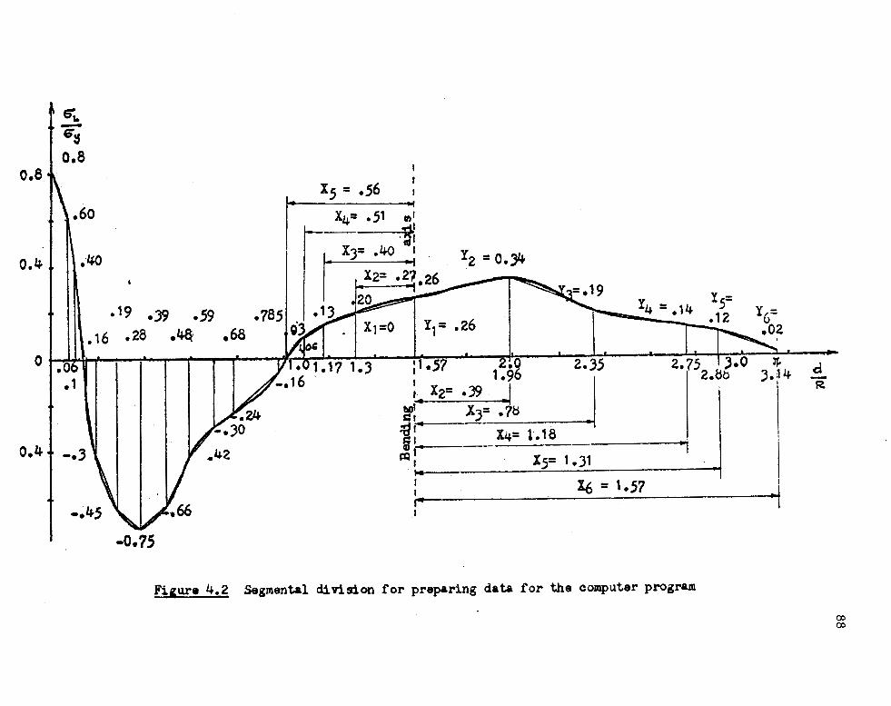
01. -6":s . o.a

o.s t\

.60

0.4 I 1 l .40 Y2 = O.J4

Y4 = .14 .l9 .39 .59 .16 .28 .4&' .68

Y1= .26

0 ~~~1__,l~--pa----..__~«..J~---L----~:1~·~57~i-..-11.~o----'-~2~.3~5"--__.~2~.7~5-+~J~.o:--_~~-----' . _ 1.96 j I 2.~o J. ~ 4 t,. X2= .')9 J

d R

o.4 + -·3

~: .X3= .7b :g1" .. i' X4= l.18

~I X5= 1.31 , .. : 16 = 1.57 r

·' -0.75

Figure 4.2 Segmental divi.sion for preparing data for the computer program

I .J ~I

00 00

89

segmental division.

The following cases give the details of the signs and quanti-

ties required as input.

Case 1. (see Figure 4.3)

Distance of center of gravity of the rectangle to Y axis:

CG! = (X1 + X2)/2

Distance of center of gravity of the triangle to Y axis:

CG2 = (2X2 + X1)/3

Area Al = (X2 - X1)/Y1

Area A2 = (X2 - X1)(Y2 - Y1)/2

Case 2. (see Figure 4.4)

Case 3.

CGl = (X1

+ X2)/2

CG2 = (2X1

+ X2)/3

Al = (X2 - x1)Y1

A2 = (X2 - x1

)(Y2 - Y1 )/2

(see Figure 4.5)

Xo = (X2 - Xl)Yl/(Y2 + Yl)

Al = X0

Y1/2

CGl = x1 + X/3

A2 = (X - X - X )Y /2 2 1 0 2

CG2 = (2X2 + xl + Xo)/3

Case 4. (see Figure 4.6)

Xo = -(X2 - Xl)Yl/(Y2 - Yl)

CGl = x1 + X/3

Al = X0

Y1/2

CG2 = (2X2 + xl + Xo)/3

90

y

Y2 Y11 IA1

0 I Xl I ' I I I I I CGl

CG2 x2

Figure 4.J Area and canter ot gravity. Case 1

y

-'1 I IY1

0 x1 x

x2

[igure 4.i Case 2

y

Y1

01 r I I '-: a a x1 CG1 :

x2

Figure 4. 5 Case )

y

CG2

x1

0

Y1

x2

Figure 4. 6 Case 4

I

Y2

91

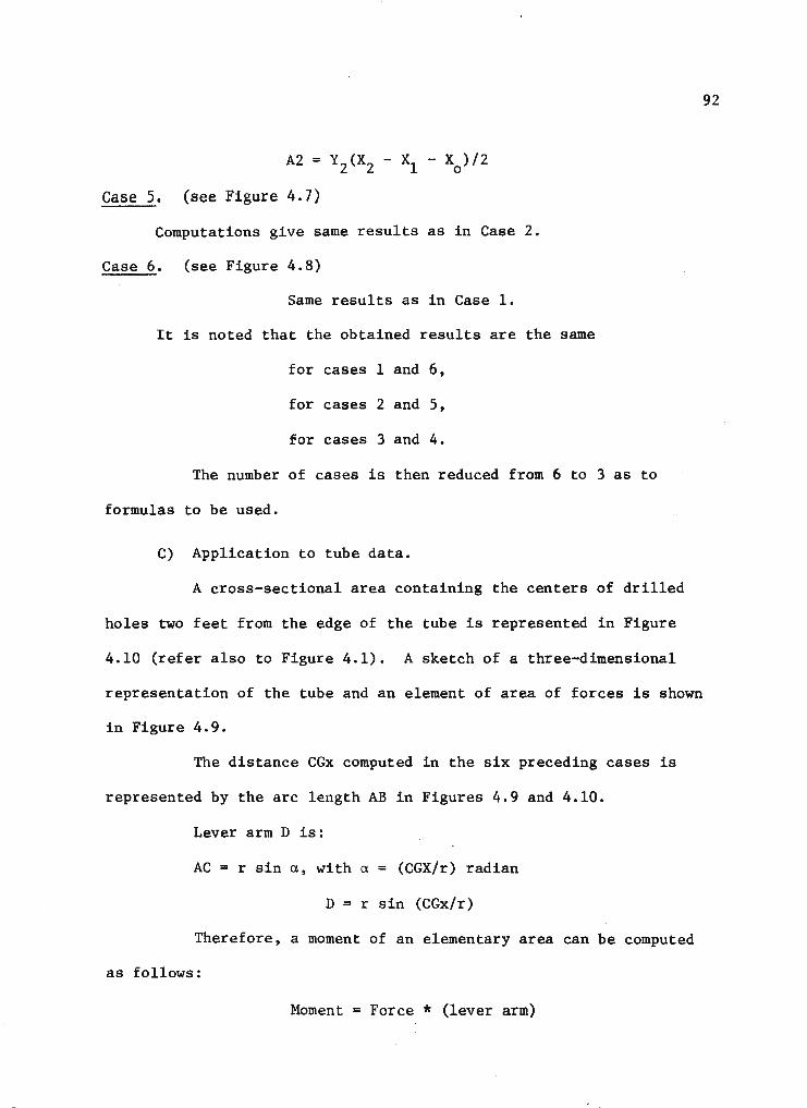
A2 = Y (X - X - X )/2 2 2 1 0

Case 5. (see Figure 4. 7)

Computations give same results as in Case 2.

Case 6. (see Figure 4.8)

Same results as in Case 1.

It is noted that the obtained results are the same

for cases 1 and 6,

for cases 2 and 5,

for cases 3 and 4.

The number of cases is then reduced from 6 to 3 as to

formulas to be used.

C) Application to tube data.

A cross-sectional area containing the centers of drilled

holes two feet from the edge of the tube is represented in Figure

4.10 (refer also to Figure 4.1). A sketch of a three-dimensional

representation of the tube and an element of area of forces is shown

in Figure 4.9.

The distance CGx computed in the six preceding cases is

represented by the arc length AB in Figures 4.9 and 4.10.

Lever arm D is:

AC = r sin a, with a = (CGX/r) radian

D = r sin (CGx/r)

Therefore, a moment of an elementary area can be computed

as follows:

Moment = Force * (lever arm)

92

93

..

y I.. x2 CGl

C02 -Xl

0 t=T I I I I r x

I I A1

11 I I I I I Y2

Figure 4.7 Case 5

y x2

C(i2 CG1

0 x Yl Al

Y2

• Figure 4.8 Case 6

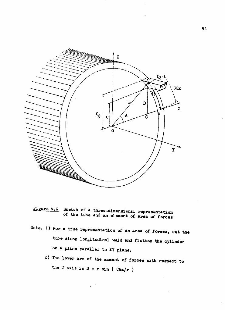
\ CGx I

Figure 4.9 Sketch of a three-dimensional repr•semtation of the tube and an element of area of f orcea

\ \

)-

z

Note. 1) For a true representation of an area o£ forces, cut the

tube along longitudinal weld and natten the cylinder

on a plane parallel to XY plane.

2) The lever arm of the moment of forces with respect to

the Z ax.is is D = r sin ( CGx/r }

94

y

A,Hole center A . . ·~ · ··Arc length

\ CGx

\ l

0 r I ~ ;·;• x

Figure 4.10 Cross-section ot the tube

.. -·· ••.. . t. t

Figure 4.11 Sketch of a volume of forces

95

m = ((X2

- x1)Y1)(r sin X + x

2 1) + 2r

((X2

- X1)(Y2 - Y1)/2)(r sin x2 + 2X1

3r )

This procedure is applied in the computer program.

D) Determination of dimensions and values for summation of

forces and moments.

1) Dimensions and values for forces.

Suppose the area of forces is a trapezoid (see Figures

4.9 and 4.11).

where:

Its area is:

Area = oL * d, with oL s (o1 + o2)/2

Volume of forces = Area * thickness

= (oL d) t

d = distance or height of the trapezoid

t = thickness of the tube

r = radius of the tube

oL = average longitudinal residual stress

a = yield stress of the steel y

As oL/oy is used in ordinate and d/R used in abscissa in

the curve (see Figures 3.27 and 4.1) the force is defined by:

let P = a r t y

0L d t p=-x-x-

o r t

p

y

Force a r t y

96

As a = 40.9 ksi y

r = 11"

t ~ 0.3125"

p .. 140.6 kip

Then, force is p * (140.6) kip

Compute yield axial force P y

1T 2 2 P • a * -(d - d ) y y 4 1

where d • 22", d1 • 21. 375", P • 670.8 kips y

97

Suppose the ratio p calculated is 0.014, the summation of forces

will be:

F • 0.014 (140.6) kips • 1.968 kips

And the ratio of summation of forces to yield axial load P is: . y

or

EF 1.9688 • 0.0022 p-- 870.8

y

F • 0.0022 P y

2) Dimensions and value for moments.

Moment of forces • Volume of forces * (lever arm)

(o1

)(d)(t)(lever arm)

The moment is defined by

01 d t

p = -x-x-x o a r t

~ y

Moment Pa = a r2t

y

2 Moment = p (a r t) 0 y

r

with

Then

0 y

r 2t = (40.9)(11)

2(0.3125)

= 1546.5 kip.in.

Moment = p * (1546.5) kip.in. 0

Suppose

Then,

or

P0

= 0.15

M = 0.15 * (1546.5) = 231.98 kip.in.

Compute Moment at first yield,

M "" s.F y y

As s • ic12t (approximate formula for the section modulus)

where d = 22", t = 0.3125"

M = (40.9)(n/4 * 222 * 0.3125) y

... 4859 kip.in.

Ratio of summation of moments to moment at first yield:

EM = My

231.98 4859 = 0.047

LM = 0.047 M y

4.1.2 Flow chart. (

A flow diagram for the computer program is shown in Figure

4.12.

4.1.3 Computer program.

98

A computer program for calculating the summation of forces and

66

o = v wns o = wwns

!'ZrTVIlINI

t•l = M 00

l-I=J

·c N)x crvmr .t.'lltr(I (1~

( OZ)l .. (OZ )'X' MCIS~CT

001

cJOJ,S

'HWllS -. ~S -7 Z!)O • l!)O

Zy • l V .r.tUlJd

M + JrOOlS = 'HNl'lS

zv +lv + vwns = n..ms Z<Jly +Lalv = M

J ' l = N m

....____-----,-____ _

... + f;

~ :.: t;1

N

--... 'cS

-0 0

+

-

-0

+ - + "' 0

f t;1 ~ K 0

--~ 0

101

CG1

CG2=0

190 170 180 150

I-' 0 N

103

summation of moments relating to measured longitudinal residual stress-

es derived from measured strains is presented in Appendix IX.

It is noted that a preparation is required for converting raw

data to input as the bending moment of the system of longitudinal

residual stresses is taken about the Z axis (see Figure 4.1). This

preparation useful for a future research presented in detail for case

1 in Appendix XI with the statement and figure defining the area of

forces limited by the curve and the Z axis.

4.1.4 Results of the computer program.

A) Results relating to stresses obtained from measured strains

with variable 4A and 4B, Table 3.11, case 1.

The output obtained from the compilation of the computer

program and data file shown in Appendix IX and relating to the initial

longitudinal residual stresses derived from measured strains with

variable 4A and 4B, case 1, Table 3.11, results in:

Summation of forces above the Z axis: -0.06 8125

Summation of forces below the Z axis: 0.0100453

Total summation of forces: -0.06 8125 + 0.100453 • 0.032328

This result is a dimensionless number. As described in

section 4.1.1.d, it must be multiplied by 140.6 kip to yield the force

to find.

EF = 0.032328 (140.6) = 4.545 kip

Expressed in percent of P , the summation of forces is: y

4.545(100)/870.8 = 0.5% of P y

-Summation of moments: -0.092374 - 0.06026 = -0.152634

104

This summation of moments must be multiplied by 1546.5 kip.in.

to yie1d inch-kips, thus:

-0.152634 (1546.5) kip.in. = -236.05 kip.in.

Expressed in percent of M , the sUilllllation of moments is: y

-236.05 (100)/4859 = -5% of M • y

Computer output and data file are given in Appenxid IX. I

B) Results related to stresses obtained from measured strains

but computed with theoretical 4A and 4B, Table 3.11, case 2.

Summation of forces above the Z axis: -0.061359

Summation of forces below the Z axis: 0.098718

Total summation of forces: -0.061359 + 0.098718 • 0.037359

Total summation of moments:

-0.086489 - 0.057948 - -0.144437

The same approach as the above one gives the final results:

Summation of forces: 0.006 P . y

Summation of moments: -0.046 M • y

Computer output and data file are given in Appendix X.

C) Results related to stresses obtained from the strain-

relaxation method with 4A and 4B, Table 3.11, case 3.

Summation of forces above the Z axis: -0.104375

Summation of forces below the Z axis: 0.085563

Total summation of forces:

-0.104375 + 0.085563 = -0.018812

Total summation of moments:

-0.088679 - 0.049973 = -0.13864

The same approach as the above one gives the final results:

Summation of forces =

Summation of moments:

-0.003 p y

-0.044 M y

Computer output and data file are given in Appendix X.

105

D) Results related to stress obtained from the strain-separation

method with 4A and 4B, Table 3.11, case 4.

Summation of forces above the Z axis: -0.043141

Summation of forces below the Z axis: 0.055731

Total summation of forces:

-0.043141 + 0.055731 - 0.01264

Total summation of moments:

-0.055679 - 0.031260 - -0.086939

The same approach as the above gives the final results:

Summation of forces: 0.002 p y

Summation of moments: -0.027 M y _

Co~puter output and data file are given in Appendix X.

These results are summarized in Table 4.1.

4.2 EVALUATION OF RESULTS

In light of the data in Table 4.1 it is seen that the results

of case 1 are marginally acceptable giving an unbalance of 10% M . y

Cases 2 and 3 have slightly better rotational equilibrium with the

smailest unbalance being 8.8% M • Case 4 gives the best results y

with 0.4% P translational and 5.4% M rotational unbalance for the y y

whole tube. This is to be expected since the calibration coefficients

for case 4 were found using a more refined technique than any of the

other cases. The unbalance present in case 4 could be attributed to

106

the choice of sector division required for data generation for the

computer program.

TABLE 4.1

RESULTS ON FORCE AND MOMENT BALANCE

Case Method Calibra- I:F I:M -- - · - - - - - - - - - - - -No. tion Half Whole Coeffi- Section Section cients

(10-8)

1 Measurement Variable 0.005 p -0.05 M 10% M y y y

2 Computation 4A=-0.86 of theoretical 0.006 p -0.046 M 9.2% M calibration 4B•-2.41 y y y

coefficients

3 Method of 4A=-0.93 strain-relaxa-

4B=-2.08 -0.003 p -0.044 M 8.8% M ti on y y y

4 Method of 4A=-1. 30 strain sep- 0.002 p -0.027 M 5.4% M aration 4B=-2.23 y y y

----·-

CHAPTER V

SUMMARY, CONCLUSION AND RECOMMENDATIONS

The experiment of drilling outside and inside holes in a welded

fabricated steel tube, according to the hole-drilling technique has

been carried out, as was the experiment of tensioning a steel plate

specimen for calibration. Longitudinal residual stresses in the tube

have been obtained from the hole drilling experiments. Calibration

coefficients used to convert data from the hole drilling experiment to

longitudinal stresses were obtained in two ways 1) Calibration coeffici­

ents were derived analytically by theory and using those recommended

by published literature, 2) Calibration coefficients have also been

computed from calibration operations performed according to the method

of strain relaxation due to drilling and the method of strain separation.

Calibration coefficients have been used in adjusting the data of the

tube. Balance of forces and moments provides a comparison of the

results of measurements and the quality of the results of refinement.

Results will be summarized, conclusion and recommendations will

be presented in the following sections.

5.1 SUMMARY OF RESULTS

The experiments of outside and inside hole drilling on the steel

tube and the calibration experiments conducted on the test plate

followed by the balancing operations of forces and moments have yielded

the following results:

A) The measured strains on the tube have shown that no further

108

strains were recorded after the values of the hole depth reached the

hole diameter value.

B) The strains measured for outside and inside holes and the

corresponding longitudinal residual stresses computed have suggested

that the stress field in the tube was well behaved through its thickness.

C) The field of longitudinal residual stresses in the tube

assumed to be uniform through its thickness, has been substantiated

by a numerical calculation using two factors of proportionality derived

from the test plate in the calibration experiment and applied to the

tube.

D) Four different kinds of calibration coefficients were used,

they are summarized as follows:

1. Variable. -8 4A = -0.83 to -1.05(10 ), 4B • -2.37 to

-2.68(10-8)

2. 4A • -0.86(10-8), 4B = -2.41(10-8 )

3. 4A = -0.93(10-8), 4B • -2.08(10-8)

4. 4A • -1.30(10-8), 4B = -2.23(10-8)

As a comparison of the accuracy of the results, a statical

equilibrium test in translation and rotation was performed for each

of the residual stress distribution obtained using the above four kinds

of calibration coefficients. The results are summarized in Table 4.1.

E) Finally, a curve plotting the most acceptable values of resi-

dual stresses based on equilibrium of forces and moments is repeated

in Figure 5.1.

5.2 CONCLUSION

The results in the preceding section show the adequacy of the

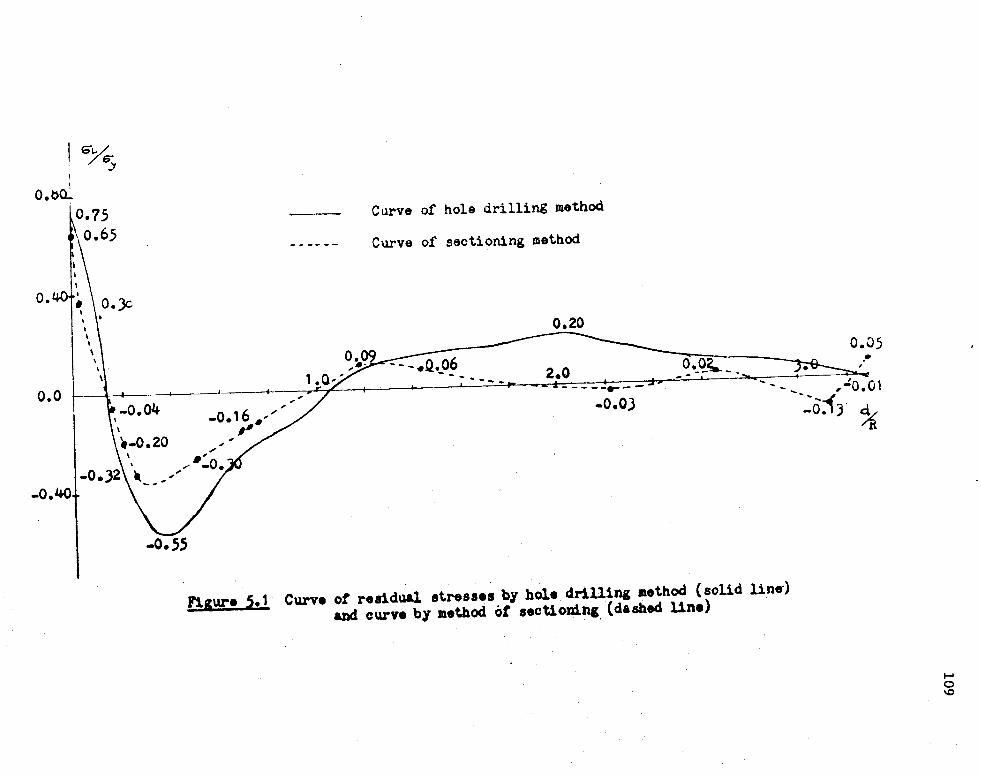
I G"i../ /~

! I

O.bcL . 0.75

o.

o.o

-0.40

o.65

\

O.)c

I

\

-0.55

c~rve of hole drilling method

Curve of sectioning method

0.20

--- 2.0 ~-_<g~--,, ____ _.. -- - --.-- -

-0.0J

Figure 5.1 · Curve or residual stresses by hole drilling method {solid line-) and curve by method ot sectioning. (dashed Un•)

0.05 .•

..:0.01 , --~o:f; ~

...... 0 ID

110

hole-drilling technique in the measurement of residual stresses,

provided the hole drilling experiments are conducted in conjunction

with the calibration carried out preferably according to strain

separation method and using material similar to the main experiment

material.

For comparison, the curve of the longitudinal residual stresses

found by the slicing method by others, is compared to the results of

this investigation in Figure 5.1.

5.3 RECOMMENDATIONS

1) Translational and rotational equilibrium calculations con-

firmed the good results of the hole-drilling strain-gage experiments

conducted on the steel tube. The curve of longitudinal r _esidual

stresses shown by a solid line in Figure 5.1 compared to results by

others, further: confirms the quality of the hole-drilling technique

in measuring residual stresses. Our first recommendation is that

calibration coefficients should always be used to refine the curve of

stresses found and the method of strain separation would be the most

efficient calibration method.

2) The solid curve shown in Figure 5.1 characterizes the dis-

tribution of residual stresses in the steel tube. For a more practical

purpose, a simplified curve comprising three straight solid lines shown

in Figure 5.2 is recommended. The balance of forces and moments

derived from the pertinent curve is obtained with a high precision

(summation of forces: -0.0005 P , summation of moments: 0.00009 M ). y . y

For comparison, a dotted straight line curve proposed by

···ill

111

Ross and Chen (5) is shown in the same Figure 5.2. This curve is a

simplified alternative of Ross and Chen presented in Figure 5.1.

A computer program applied to this simplified curve with the same con-

ditions as for the simplified curve of our tube, shows that the pre-

cision obtained in balancing forces and moments was equivalent:

Summation of forces: -0.00012 P (against -0.0005 P for our curve) y y

Summation of moments: 0.0026 M (against 0.00009 M for our curve) y y

Finally, our simplified straight line approximation presented

in Figure 5.2 to represent longitudinal residual stresses in the steel

tube, is recounnended for use in further studies of the effects of re-

sidual stresses on failure loads.

1.00

0.80

0.40·

o.o

0.40

01../c. y

I

I I

I I

Curve of hole drilling method

Curve of sectioning method

I \ \ . ;;r ~' 1 • q_ ...', ~ - - ------- --., • .3. 0 0.1.S \ ,, /

1

:.d/R

' ' \ ' ' ',.-

-0. J ....

,,c 2.0 ,,c

, ..

-0.4

Fi1ur• s.2 Ross and Chen sillplltied CurYe by sectionin& aethod (dotted line) and simplified curTe by hole-drilling method (eolld line) to

represent residual stresses.

-0.08

I-' I-' N

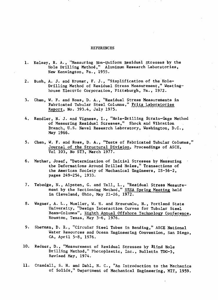
REFERENCES

1. Kelsey, R. A., "Measuring N:>n-Uniform Residual Stresses by the Hole Drilling Method," Aluminum Research Laboratories, New Kensington, Pa., 1955.

2. Bush, A. J. and Kromer, F. J., "Simplification of the Hole­Drilling Method of Residual Stress Measurement," Westing­house Electric Corporation, Pittsburgh, Pa., 1972.

3. Chen, W. F. and Ross, D. A., "Residual Stress Measurements in Fabricated Tubular Steel Columns," Fritz Laboratories Report, No. 393.4, July 1975.

4. Rendler, N. J. and Vigness, I., "Hole-Drilling Strain-Gage Method of Measuring Residual Stresses," Shock and Vibration Branch, U.S. Naval Research Laboratory, Washington, D.C., May 1966.

5. Chen, W. F. and Ross, D. A., "Tests of Fabricated Tubular Columns," Journal of the Structural Division, Proceedings of ASCE, Vol 103, No ST3, March 1977.

6. Mathar, Josef, "Determination of Initial Stresses by Measuring the Deformations Around Drilled Holes," Transactions of the American Society of Mechanical Engineers, IS-56-2, pages 249-254, 1933.

7. Tebedge, N., Alpsten, G. and Tall, L., "Residual Stress Measure­ment by the Sectioning Method," SESA Spring Meeting held in Cleveland, Ohio, May 21-26, 1972.

8. Wagner, A. L., Mueller, W. H. and Erzurumlu, H., Portland State University, "Design Interaction Curves for Tubular Steel Beam-Columns", Eighth Annual Offshore Technology Conference, Houston, Texas, May 3-6, 1976.

9. Sherman, D.R., "Circular Steel Tubes in Bending," ASCE National Water Resources and Ocean Engineering Convention, San Diego, CA, April 5-8, 1976.

10. Redner, D., "Measurement of Residual Stresses by Blind Hole Drilling Method," Photoplastic, Inc., Bulletin TDG-5, Revised May, 1974.

11. Crandall, S. H. and Dahl, N. C ~ , "An Introduction to the Mechanics of Solids," Department of Mechanical Engineering, MIT, 1959.

12. "RS-200 Milling Guide, a Precision Optical Alignment and Guide tool for Measurement of Residual Stresses by the Strain Gage Hole Drilling Method, 11 Photolastic, Inc., Bulletin S-105, 1976.

13. Chaj es, A., "Principle of Structural S.tability Theory," Department of Civil Engineering, University of Massachusetts, 1974.

14. Beedle, L. S., "Plastic Design of Steel . Frames," Research

114

Professor of Civil Engineering, Fritz Engineering Laboratory, Department of Civil Engineering, Lehigh University, 1958.

15. Wagner, A. L., "A Numerical Solution for the Ultimate Strength of Tubular Beam-Columns," Masters Thesis, Portland State University, Nov. 1976.

16. Chen, W. F. and Ross, D. A., "Behavior of Fabricated Tubular Columns under Biaxial Bending," ASCE National Water Resources and Ocean Engineering Convention, San Diego, CA, April 5-8, 1976.

..

APPENDIX I

DERIVATION OF EQUATIONS (3)

(A + B cos 2$) E - (A - B cos 2$) E a c o =

1 4AB cos 2$

(3)

(A + B cos 2$) E - ( A - B cos 2$) E c a a = 2 4AB cos 28

tan 2$ = E - 2Eb + E a c

E - E a c

In section 2.2.2, the following expression has been established

Er= [A+ B cos 2a) o1 + [A+ B cos 2(a + 90)) o2

Extending to directions a and c, and replacing a by $, it becomes =

Ea= [A+ B cos 2$) o1 + [A+ B cos 2($ + 90)) o2 (2a)

Ec = [A+ B cos 2($ + 90)] o1

+[A+ B cos 2($ + 180)) o2

Noting that

cos 2($ + 90) = cos (2$ + 180) = -cos 2$

cos 2($ + 180) = cos (2$ + 360) = cos 28

(2a) can be rewritten =

[A + B cos 2$] a1

+ [A - B cos 2$] a2 = ea

(2b) [A - B cos 28] a

1 + [A + B cos 28] a 2 = ec

Dividing both members by the coefficients of o1 =

0 + A - B cos 2$

£ a a = 1 A + B cos 28 2 A + B cos 28

0 + A + B cos 2$

£ c a = 1 A - B cos 2$ 2 A - B cos 2$

Using direct elimination (subtract member to member) =

cos 2$ A + B cos 28 ea A - B cos 2$) 0 2 = _A __ + __ B-=c-o_s __ 2_8 (A+ B

A - B cos 2~

Developing and rearranging terms =

£ c A - B cos 2$

116

2 2 [(A - B cos 28) -(A+ B cos 2$) a~= £ (A - B cos 26)- £ (A+ B cos 26) .... a c

[-2 AB cos 2$ - 2 AB cos 2$] o2 = e (A - B cos 26)- e (A+ B cos 26) a c

Finally:

(A + B cos 2$) e - (A - B cos 26) e c a 0 = 2 4 AB cos 2$

With the same approach =

(A + B cos 28) e - (A - B cos 28) e a c a = 1 4 AB cos 28

Proof of =

tan 213 = e: - 2 e:b + e: a c

e: - £ a c

Remind =

e:a = [A + B cos 213] a1 + [A - B cos 213] a2 (2b)

e:c = [A - B cos 213] a1 + [A + B cos 213] a2

then = e:a + e:c = 2 A(al + a2)

(2c) e:a - e:c = 2 B cos 213(a1 - a 2)

therefore =

e: - e: a c cos 213 = 2 B (al - a2)

Calculate sin 213.

For direction b =

e:b = [A+ B cos 2(8 + 45°)] a1 + [A+ B cos 2(8 + 135°)] a2

e:b = [A - B sin 213] a1 + [A + B sin 26] a2

e:b = A (a1 + a 2) + B (a 2 - a 1) sin 28

Therefore =

sin 28 A (al + a2) - e:b

B (a2 - a 1)

117

tan 2S

Compute tan 2S:

sin 2f3 cos 2f3

A(al + a2) - E:b

B(a2 - a1)

2A(a 1 + a 2) - 2Eb

E - E a c

x 2B(al - a2)

E - E a c

As 2A(o 1 + a 2) = Ea + Ee' from (2c)

Finally:

E + E - Eeb tan 2f3 = a c

E - E a c

E - 2Eb + EC a E - E a c

118

120

Developing and rearranging terms =

(A - B cos 2S)(A - B sin 28) (A+ B sin 2S)(A + B cos 2B) a2 =

Ea (A - B sin 2B) - ~b (A + B cos 28)

Developing first member

2 e I A - AB sin 2B - AB cos 2B + Bi sin 28 cos 2B

-(A2 + AB cos 28 + AB sin 2B + B2 sin 28 cos 2S) =

-2AB (sin 28 + cos 28)

Then=

a = 2

(A + B cos 28) Eb - (A - ~ sin 2B, Ea

2AB (sin 2B + cos 2B) I

With the same approach =

0 =(A+ B sin 28) Ea - (A - !B cos 2Bl) Eb

1 2AB (sin 2B + cos 28)

APPENDIX II I

DERIVATION OF EQUATIONS (3a)

s D 0 1 = 4A + 4B cos 26

(3a) s D Oz =- - 4B cos 26 4A

s - 2£b with tan 26 = --D

s = £ + £ a c

D = £ - £ a c

(3)

0 = 1

=

Rewrite equation (3) from Appendix I

(A + B cos 26) £ - (A - B cos 26) £ a c

0 = 1 4.AB cos 26

(A + B cos 26) £ - (A - B cos 26) £ o2 = c a

4AB cos 26 -

Developing the second member and grouping terms =

A (£ - £ ) + B cos 26 (£ + £ ) a c a c

£ + £ a c 4A +

4AB cos 26

£ - £ a c

4B cos 26

122

- 2_ + D 0 1 - 4A 4B cos 2B

With the same approach

S D a = - -2 4A 4B cos 2B

Coefficients 4A and 4B can be computed by adding or subtracting

member to member, from equations (3a)

2S 4A =

al+ 02

2D 4B = ( 0 _ a ) cos 2B

1 2

ED DOCK

..

APPENDIX IV

COMPUTER PROGRAM FOR CALCULATING PRINCIPAL STRESSES 01 & 02 WHEN STRAINS

£A , £B , £C ARE KNOWN

1 READC7r4>EArEBrEC 2 4 FORMAT<3E7.0> 3 S=EA+EC 4 D=EA-EC 5 WRITEC18r6>SrD 6 6 7 8 8 9 10 11 12 10 13 14 1 C"

• ..J

16 1? 20 18 19 EDF •• EDT ••

FORMAT<5X'SUM S='E15.6r5X'DIFF D='E15.6) READC7r8>F4ArF4B FORMATC2E7.2) C=ATAN<<S-2*EB>ID>

Cl=C*lB0./3.14159 WRITEC18r10)C1 FORMATC5X'ANGLE 2B='F8.2> BCOS=COS<C> Sl=S/CF4A>tD/CF4B*BCOS> S2=S/CF4A>-Dl<F4B*BCOS) WRITE(18r20>SlrS2 FORMAT<3X'STRESS l='F11.2r3X'STRESS 2='F11.2> STOP END

DATA FILE AND OUTPUT

ED DOC3

1 +004E-6+027E-6+075E-6 2 -132E-8-220E-8 3 EDF EOT ••

FR 5,6 FO. WNME, I•OCK AS 18=*3 AS "7=DOC3

.vx.N

124

SUM S= 0.790000E-04 DIFF D= -0.710000E~04 ANGLE 2B= -19.40

STRESS 1= -2563+36 ) STRESS 2= _ -9406~34 STOP

: .•..

APPENDIX V

Graphical method using a stress MOHR's CIRCLE to determine

longitudinal and circumferential stresses crL & crT when principal

stresses cr1

& a2

are known.

Build the stress Mohr's circle with diameter AB, ~bscissa OA • cr1

and abscissa OB = cr2 .

The direction e of gage a with respect to cr1 is given by formula

s - 2£ b tan 2e = D

If the direction b coincides with the transverse axis of the pipe, and

a is the angle of the longitudinal axis with direction cr1 :

a = 90° - (45° + S) = 45° - e

In the Mohr's circle, the angle used for a direction is double: (see Fig. A.6.1)

2a = 90° - 2e

Knowing the direction of cr 1 on the Mohr's circle (radius wA), open

an angle AwC = 2a = 90° - 26, the abscissa of M,intersection with the

circle is the longitudinal stress cr1 •

The abscissa of Point N diametrically opposite to M is the trans-

verse or circumferential stress crT.

"'-·

AE.E,lication. Hole 1.

£ = 4 £b = 27, £ = 75 a • c

o1 = -6070 psi, o2 = -12091 psi

213 = 19° 22 a = 9° 41

a = 90° - (45 + 9.41) z 35° 19

2a = 70° 38

Build a Mohr's circle with =

OB = -12091 psi

OA = -6070 psi

126

·-..

From wA, open an angle AwC = 2c( = 70° 38; its second side cuts th.e circle

in points M & N.

Point M, o1 = -8080 psi

Point N, OT = -10090 psi.

APPEUDIX VI

COMPUTER PROGRAM

ANALYTICAL STUDY

Determination of longitudinal stress oL and circumferential stress

oT when principal stresses o1 and o 2 are known.

Part I. Longitudinal Stress gL.

Equation of a Mohr's circle of stress, when principal stresses o 1 ,

o 2 are known:

T

r 02 m (J

B 0 0 A n D:

OL

: d= (o · +a )/2 I 2 1 '-- ----------- --- - -- --I

Figure A.6.1. Stress Mohr's circle.

(1) 2 2 2

(X - OD) + Y = r

As OD = d = (J 2 - 01

2

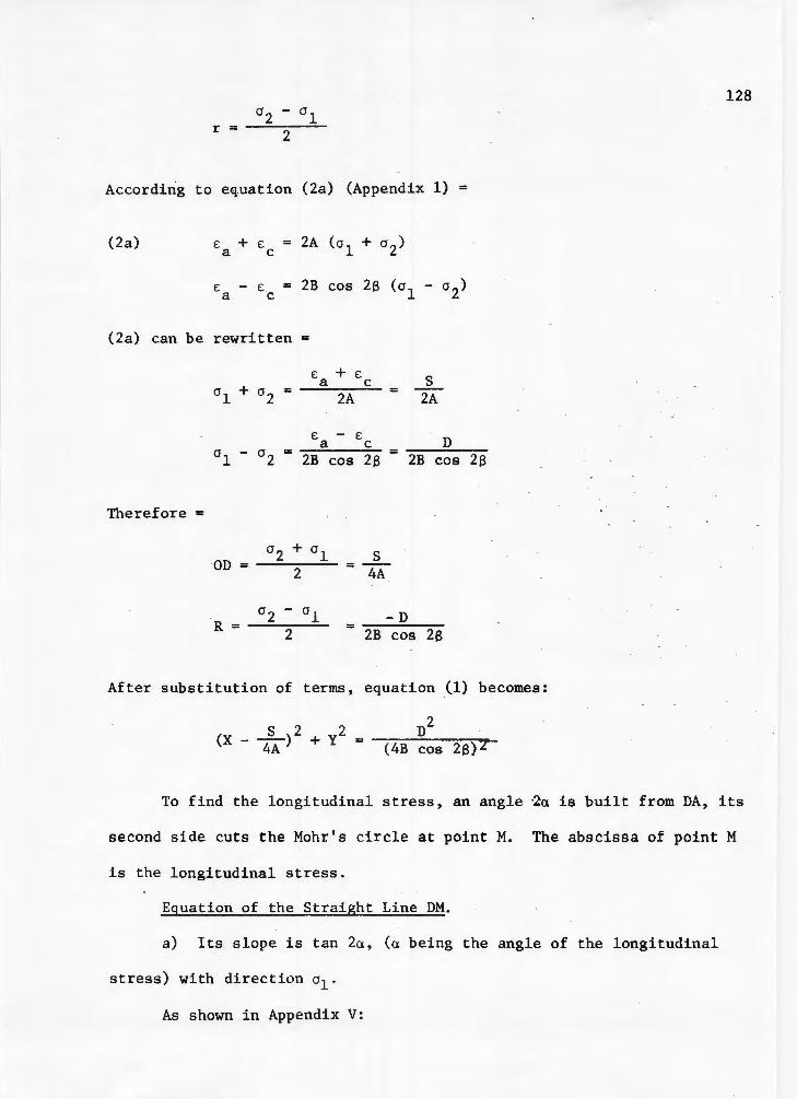
r = a2 - ol

2

Accordi~g to e~uation (2a) (Appendix 1) =

(2a) E: + E: a c

E: - E: a c

2A (o1 + o2)

2B cos 2S (o1 - o2)

(2a) can be rewritten =

E: + E: s 01 + 02 =

a c = 2A 2A

E: - E: D a c a - a = = 1 2 2B cos 2S 2B cos 2S

Therefore =

02 + 01 s OD = 2 = 4A

oz - al -D R = 2 = 2B cos 2S

After substitution of terms, equation (1) becomes:

2 S 2 2 - __ ..::,D:__~~~

(X - 4A) + y - (4B cos 2S)Z--

128

To find the longitudinal stress, an angle ·2a is built from DA, its

second side cuts the Mohr's circle at point M. The abscissa of point M

is the longitudinal stress.

Equation of the Straight Line DM.

a) Its slope is tan 2a, (a being the angle of the longitudinal

stress) with direction o1 .

As shown in Appendix V:

a = 45° - 8

2a = 90° - 28

tan 2a = tan (90° - 28)

= cotan 28

1 tan 28

According to equation (3), Appendix I,

tan 28 =

Let M =

Then

tan 2a

s - 2e:b

D

s - 2£b

D

1 D 1 tan 28 = S - 2£b = ~-M

b) As the straight line passes through point D (abcissa •

0 2 + 0 1 2

- s - 4A • ordinate = O)

1 Y=-X+N M

M = s - 2~1:>

D

D S O = ( S - 2£b ) 4A + N

N = -SD 4A (S - 2£b)

D SD y = ( S - 2£b )X - 4A (S - 2£b)

1 s 1 Y=-x--x-M 4A M

129

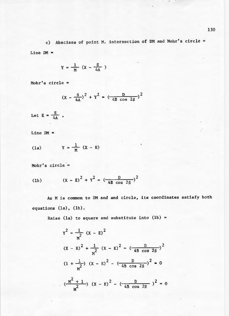
c) Abscissa of point M. intersection of DM and Mohr's circle =

Line DM =

1 s ) y = M (X - 4A

Mohr's circle

(X - _S_)2 2 4A + Y =

s Let E = 4A '

Line DM =

(la) 1

Y = - (X - E) M

Mohr's circle=

( 4B D

cos 2

2B )

(lb) (X - E)2 + y2 = ( D )2 4B cos 2B

130

As M is conunon to DM and and circle, its coordinates satisfy both

equations (la), (lb).

Raise (la) to square and substitute into (lb) =

2 1 2 y = - 2 (X - E) M

2 1 2 - D )2 (X - E) + -2 (X - E) - ( 4B cos 2f3

M

1 2 D )2 = 0 (1 + - 2 ) (X - E) - ( 4B cos 2f3 M

M2 + 1 2 ( D )2 = 0 ( 2 ) (X - E) - 4B cos 2f3 M

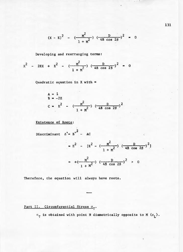
(X - E) 2 2 .

( M ) ( D )2 = 0 -l + M2 4B cos 28

Developing and rearranging terms:

x2 2EX E2 M2 D 2 0 - + - ( 0 ) ( 4B cos 28 ) = 1 +ML

Quadratic equation in X with =

A= 1 B = -2E

E2 M2 D )2 c "" - ( 2 ) ( 4B cos 28

1 + M

Existence of Roots:

Discriminant ~

ll' = B' - AC

2· = E M2 D

[E2

- ( 2 ) ( 4B cos 1 + M

2 = +( M ) ( D 2

1 + M2 4B cos 28 ) > 0

Therefore, the equation will always have roots.

Part II. Circumferential Stress aT.

2 28 ) ]

0T is obtained with point N diametrically opposite to M (aL).

131

132

COMPUTER PROGRAM

for longitudinal and circumferential stresses

E:O SIGMA.-'.i

1 READ( 7 ?4>EAvEB,EC 2 4 FORMATC3E7.0> 3 S=E A+EC 4 D=EA-EC 5 WRITEC18,6>EAvEB,EC 6 6 FORMAT<5X'EA='E15.4,5X'EB='E15.4,5X'EC='E15.4) 7 READ<7,8>F4A,F4B 8 8 FORMAT<2E7.2) 9 WRITEC18,9>F4A,F4B 10 9 FORMATC5X'F4A='E15.4,5X'F4B='E15.4) 11 Q=S/CF4A> 12 XM=<S-2.*EB)/D 13 XL =ATAN<XM> :1.4 1 ~ ~ 16 10 17 18 c 19 20

Xll=XL*lB0./3.14159 WRITEC18,10>XL1 FORMATC5X'ANGLE XL1='F8.2> BCOS=COSCXL> COMPUTE STRESS 1 AND STRESS 2 S1=S/CF4A>+D/CF4B*BCOS> S2=S/CF4A) - D/CF4B*BCOS>

21 WRITE<18v12)S1,S2 22 12 FORMAT<3X'STRESS 1='F11.2,3X'STRESS 2='F11.2) 23 C COMPLJTE'LONGITLJDINAL STRESS' 2 4 A=l ,.) C!'" ,,,; .. '-J

26 :~·7

28

B=- 2.*Q C=Q**2 - CXM**2/C:J..+XM*XM>>*<D/((F4B>*BCOS>>**2 TEMP=B**2-4.*A*C IFCS1)30v30Y60

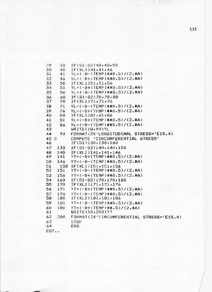
2 9 30 30 40 3:1. 4:1. 3 :~ 46 33 ~50 34 !'.'i l :·5!5 ~.'iii

36 60 ::p 70 38 ?1 39 76 40 80 41 8:1. 4 ':> •.. 86 43 44 90 4:'.'j c 46 47 l 30 48 l.40 49 :1.41 ~50 :1.46 ~51. 150 1;.-,., .... J.:.. 1 ~):I. 53 1!:-}6 ~54 160 c:.·c· ~ .. , 170 56 171 57 :1. 7,s 58 :I.BO ~59 181 60 :l.B6 61 62 :?oo 63 ,~4

EDT ••

I F< S1-S2 )4Q,40,50 IF ( XI ... I. ) 4 :l. , 4 :I. , 4 6 YL = C- B- CTEMP)**0.5)/(2.*A> YL=C - B+<TEMP>**0.5)/(2.*A> I F ( Xl...1 ) ~5 l , !'.'i l , ~'i6 YL =C-B +CTEMP>**0 , 5)/(2.*A> YL =<- B-<TEMP>**0.5)/(2.*A> IF<S1 - S2>70,70r80 IF(Xl...:I. 17:1. ,71,76 YL = <-B - <TEMP>**0.5)/(2.*A> YL=< - B+<TEMP>**0.5)/(2.*A> IF (XI ... :I. ) 8 :I. , 81, 86 YL =<- B+<TEMP>**0.5)/(2.*A> Yl =<- B-<TEMP>**0.5)/(2.*A> WIU TE< :LB, 90) YL.. FDRMATC2X'l...DNGITUDINAL STRESS='E15.4> COMPUTE 'CIRCUMFERENTIAL STRESS' IF<Sl):l.30,:1.30,160 IF< S1- S2>140,l40,150 IFCXl...1)14l,:t.41r146 YT=< - B+<TEMP>**0.5)/(2.*A> YT =<- B- <TEMP>**0.5)/(2.*A> IFCXl...:1.)15:1.,:1.5:1.,:1.56 YT=< - B-<TEMP>**0.5)/(2.*A> YT =<- B+<TEMP>**0.5)/(2.*A> IF<S1 - S2>1 70,:J.70,180 IF<XL:l.):1.71,:1.71,176 YT=< - B+<TEMP>**0.5)/(2.*A> YT =<- B- <T EMP>**0.5)/(2.*A> IFCXl...1)18:1.,:1.81,:1.86 YT = C-B-<TEMP>**0.5)/(2+*A> YT=C- Bt<TEMP>**•5)/(2.*A> WI~ I TE< :l 8, 200 >YT FDRMATC2X'CIRCUMFERENTIAL.. STRESS='E15.4) ~:; TOP

END

133

DATA FILE AND OUTPUT

for longitudinal and circumferential stresses

ED DOCK3

1 t004E-6+027E-6t075E-6 2 - 087E - 8 - 250E-8 3 EDF EOT ••

FO.WNME,SIGMA6 AS 18=*3 AS 7 =DOCK3 vx.N

EA= F4A=

0.4.000E-05 -0.8700E-08

ANGLE XL1= -19.40

EB= F4B=

0.2700E-04 -0.2500E-07

STRESS 1= -6069.55 STRESS 2= -12091.37 LONGITUDINAL STRESS= -0.1008Et05 CIRCUMFERENTIAL STRESS= -0.8080Et04

STOP

EC= 0.7500E-04

I-" w ~

•

APPENDIX VII

Graphical method to determine longitudinal and circumferential

strains £L & £T, when strains £a' £b' £c are known.

A. Construct Mohr's circle.

Build a system of orthogonal coordinates:

-vertical axis or axis of half shear-strains.

-horizontal axis or axis of strains (see Figure A7.l)

On the axis of strains, plot:

OA = £ a

OB = £b

oc = £ c

Mark point D middle of AC. On the .verticals of A and C, build:

Aa = BD Cc = BD

aD and De are the radii of Mohr's circle.

On the vertical of B, build:

Bb = DA . o r Bb = DC

Db is also the radius of the circ le. The three right angles aAD, cCD and

bBD are equal.

Draw the Mohr's circle passing on a, b, c.

; ·~ ..

Half shear strain

~

0 I J I rt u: I ~t.c I I I I

c

M

Figure A.7.1. Strain Mohr's circle

E:

strains

136

Note the location of points I and II giving the maximum and

minimum strains £ 1 and £ 2.

B. Check location of directions (gages) a, b, c.

As the three directions a, b, c are 45° apart and counterclock-

wise, the three points a, b, c on the Mohr's circle 90° apart (double

angle in Mohr's circle) and counterclockwise are good ones.

and

C. Compute the longitudinal strain.

1.) In Appendix V =

Cl = 45° - 8

tan 2'3 s - 2 e:b

D (Appendix I)

137

The angle of principal axis £1

with e:1 is 2Cl, in Mohr's circle =

2Cl = 90° - 28

The second side of the angle 2a built from the principal strain

direction cuts the Mohr's circle at point M, its abscissa is the longi-

tudinal strain.

2.) Numerical example.

Case of Hole 1 .

Strains £ a

4 x 10-6 , £ = b

Plots points A, B, C on strain axis:

OA = 4 OB 27

27 x 10-6 , £ c

-6 = 75 x 10 .

oc = 75

Mark point D,middle of AC.

Build Aa = Cc = BD = 13 .

Draw the strain Mohr's circle from D with radius OD= 37.5.

Compute tan 2t3

=

2t3 = -19° 24 mi

4 - 2(27) + 75 4-75

25 -71

t3 = _90 24mi

2a = 90° - 2 t3 = 70° 18mi

mi From the principal axis, open an angle 2a = 70° 18 · , its second side

cuts the Mohr's circle, first at point M then, at point N.

-6 Longitudinal strain om = 27 x 10 •

Circumferential strain on= 52 x 10-6 •

-

138

APPENDIX VIII

COMPUTER PROGRAM

VIII A. ANALYTICAL APPROACH

A. General Considerations

The construction of a strain Mohr's circle has been shown in

Appendix VII.

The problem consists of determining the directions and magnitudes

of the longitudinal and circumferential strains when the angle a of the

direction a with the longitudinal direction is known (B = angle of direc-

tion a with principal axis).

Let:

o = a - B

In the strain Mohr's circle, double angles are considered

2o = 2a - 28

As tan 2B can be determined by equation (3) and .tan 2a is known, 2o can

be calculated.

tan 2o = tan (2a - 28)

(1) tan 2o = tan 2a - tan 2B 1 + tan 2a tan 28

B. Equation of Strain Mohr's Circle (See Fig. A7.l)

In strain Mohr's circle, are known =

£ =OA a

£b = OB

£ = oc c

For convenience's sake, let OA =a OB = b oc = c

Then OC = d = a+ c 2

Radius of Mohr's circle =

R2 ,.. BD2 + Bb 2

As Bb = DC = c - d

a+ c =c---2

Bb = c - a

2

BD = d - b = a+ c 2

Let S = a + c

D = a - c

- b =

R2 = ( c - a )2 + ( a + c - 2b )2 2 2

cl> 2 + c s - 2b > 2 2 2

Equation of the strain Mohr's circle

a + c - 2b 2

(X _ a! c)2 + y2 = -t- [D2 + (S _ 2b)2]

;·· ··

140

141

Let Q = S - 2b

(X _ ~S~)2 + y2 = ~1- (D2 + Q2) 2 4

C. Equation of the Straight Line DM.

Y = MX + N

If 2o is the angle of the principal direction and the longitudinal

direction, its second side cuts Mohr's circle at point M, its abscissa

is the value of the longitudinal strain.

The slope of DM is tan 2o which can be computed by the equation (1)

Y = tan 2o X + N

a + c As the line DM passes through point D ( 2 , O), the coordin-

ates of D satisfy this equation: (See Figure A.7.1)

Then:

s o = tan 2o ( - 2- ) + N

s N = - --- tan 28 2

s Y = tan 2o (X - -)

2

D. Magnitude of Longitudinal Strain

As M is conunon to the line and the circle, its coordinates satisfy

both equations.:

(la) Line: Y

(lb) Circle:

s tan 2o (X - -2-)

(X __ S_)2 + y2 = _.l_(D2 + Q2) 2 4

Raise (la) to square and substitute into (lb):

2 s Y = tan 2o (X - --2--)

(X ___ s __ )2 + tan2 28 (~ ___ s __ )2 = __ 1 __ (D2 + Q2) 2 2 4

or

2 s 2 1 2 2 (1 +tan 2o)(X - --2--) - --4-- (D + Q) = 0

or

2

(X - -t-) (D2 + Q2) = 0

4(1 + tan2 2o)

Developing and rearranging terms =

x2 2 (D2 + Q2)

sx + + - 4 (1 + tan2 2o)

Quadratic equation in X where

Discussion

A= l

B = -S 2

c =-s-4 -(D

2 + D 4(1 + tan2 2o)

a) Condition of root existence:

2 ~ = B - 4AC > 0.

0

b) When angle 2o < 90°, the longitudinal strain equals:

E: = x = L 1

v 2 -B - B - 4 AC

2A

142

£f]1

VIII B

COMPUTER PROGRAM

for longitudinal and circumferential strains.

ED EPSIL3

1 2 3 4 5 6 7 6 8 9 7 10 11 12 13 14 15 16 17

4

8

READ(7,4>EA,EB,EC FORMAT<3F7.0) S=EA+EC D=EA-EC Q=EA+EC-2.*EB WRITE<18.6)S,rr,o FORMAT<2X'SUM S='E15.4,2X,'DIFF D='E1S.4,2X,'SUM- 2EB='E15.4> READC7,7>F2A FORMATCF6.2>

T=TANCF2A> R=<S-2.*EB>ID F2B=ATAN<R> F2B1=F2B*180./3.14159 F2D=F2A-F2B1 WRITEC18,8>F2D FORMATC2X'ANGLE 2D='F6.2> Y=<T-R)/(1.+T*R>

..... ~ ~

•

18 19 20 21 22 9 23 24 25 26 10 27 c 28 60 29 70 30 80 31 32 90 33 c 34 35 160 36 170 37 180 38 39 190 40 300 41 EOT ••

A=1. B=-S C=CS**2>/4.-CD**2+0**2)/(4.*C1.tCY>**2>> WRITE<18,9)A,.B,C FORMATC4X'A='E15.4,4X'B='E15.4,4X'C=' E15.4> TEMF' =B**2 ·- 4. *A*C XM=Y IFCTEMP>300,10,10 IFCXM>S0,70,60 COMPUTE"LONGITUDINAL STRAINM ZL =C- Bt<TEMP>**0.5)/(2 . *A> ZL. :::·-B/ ( 2 •*A) ZL=< - B- CTEMP>**0.5)/(2.*A> WRITE<1B,90)Zl.. FORMATC2X"LONGITUDINAL STRAIN="E15.4) COMPUTE·CIRCUMFERENTIAL STRAINM IFCXM>180,170,160

ZT=<-B- CTEMP>**0.5)/(2.*A> ZT=- B/(2.*A>

ZT =<-B+<TEMP>**0.5)/C2.*A> WRITE<l8,190>ZT FORMATC2X'CIRCUMFERENTIAL STRAIN='E15.4> STOP END

...... +:­Vl

VIII C

DATA FILE AND OUTPUT

for longitudinal and circumferential strains.

ED APE:I.

1 +004E- 6t027E-6+075E-6 2 109.20 3 EOF EOT ••

FR 5,6 FD.WNME,EPSIL3 AS 18==*3 AS 7=APE1 VX.N

SUM S= 0.7900E-04 DIFF D= -0.7100E-04 SUM-2EB= 0.2500E-04 ANGLE 2D=128.60

A= o.1000E+o1 B= -0.7900E-04 C= 0.3763E-09 LONGITUDINAL STRAIN= 0.5092E-05 CIRCUMFERENTIAL STRAIN= 0.7391E-04

STOP

..... ~ (J\

APPENDIX IX

IX A. COMPUTER PROGRAM for force and moment balance.

ED HETF<:I.

1 DIMENSION XC20)?YC20) 2 READC:f.2,10>I~J,R,T,DC

3 10 FORMATC213,3F12.4> 4 READ<12v20><X<N>,N=:f.,I) 5 20 FORMATCF11.3> 6 WRITEC18Y30) 7 K=I-1 8 DO 240 M = 1~ J

9 SUMM=O.O 10 SUMA=O.O 11 30 FORMATC2X' AREA1 LEVER ARM 12 1 SUM MOMENTS') 13 READ<12,40>CYCN),N =1,I) 14 4 0 FORMATCF11.3) 15 16 17 18 19 20

DO 240 N=1,K IF<Y<N>>l00,90,110

90 IF<Y<Ntl)):f.80,95,180 95 Al=O+O

A2=0.0 CG1=0+0

21 CG2=0.0 22 GO TO 220 23 100 IFCYCN+1>>120,190,170

AREA 2 LEVER Ai:;:M SUM FClr<CES

.....

.!:­

.......

' ~

24 110 IF' CYCNt1))170,190r130 25 120 IF<Y<Nt1)-Y(N))150,135,140 26 130 IF<Y<Nt1>-Y<N>>140r135v150 T7 135 Al=<X<N+i>-X<N>>*Y<N> 28 CGi=CXCNtl>+X<N>)/2.0 r)\' .· .. ')' A2====0. 0 30 CG2=0.0 31 GO TO 220 32 140 CGl=CXCN+l>tXCN))/2.0 33 CG2=CXCN+1>+2.0*XCN))/3.0 34 A1=<X<Nt1>-X<N>>*Y<N+1> 35 A2=CX<N+1>-X<N>>*<Y<N>-Y<Nt1))/2.0 36 GO TO 220 37 150 CG1=CXCN+1>+X<N>>l2.0 38 CG2= CXCN+1>*2.0+X<N>>l3.0 39 A1=CXCN+1>-X<N>>*Y<N> 40 A2=CXCNt1>-X<N>>*<Y<N+1>-Y<N>>l2+0 41 GO TO 220 42 170 XO=CX<N+1>-X<N>>*<-Y<N))/CYCN+1>-Y<N>> 43 CG1=CX0/3.0>+X<N> 44 CG2=<2.0*X<N+1>tXCN)tX0)/3.0 45 A1=<XO*Y<N>>l2.0 46 A2=CX<N+1>-<X<N>+XO>>*Y<Nt1>/2.0 47 GO TO 220 48 180 CG1=<2.0*X<Nt1>+X<N>>l3.0 49 CG2=0.0 50 A1=<X<Nt1>-X<N>>*Y<Nt1)/2.0 51 A2=0.0 52 GO TO 220 53 190 CG1=<X<N+1>t2.0*X<N>>l3.0 54 CG2=0.0 55 Al=CX<N+1>-X<N>>*Y<N>l2+0 56 A2=0.0

....

.i:--00

57 22 0 A1 =A1*T 58 A2= A2*T 59 IFCCG1 )222 ,221,222 60 221 Dl =O.O 61 GO TO 223 62 222 D1 =R*SIN<CG1/R)-DC 63 223 IF<CG2)225Y224Y225 64 224 D2=0.0 65 GO TO 226 66 225 D2=R*S IN<CG2/R> - DC 67 226 XM=A1*D1tA2*D2 68 S UMA =SUMA+A1+A 2 69 SUMM=SUMM+XM 70 WRITEC18, 230)A1YD1 rA2,D2YS LJMA ,S UMM 71 230 FORMATC6E13.6) 72 240 CONTINUE ..... 7 /,.,

74 "75 76 77 78 79 80 81 82 83 84 85 86 87 88 89

READ C12 , 2>IrJ vR,f , DC 2 FORMAT<2I 3 ,3F12.4)

READ<1214)CX<N>,N=1•I> 4 FORMATCF11.3)

K=I-1 DO 340 M=l,J SUMM =O.O SUMA =O.O WRITE<18,6)

6 FORMATC2X' AERA 1 LEVER ARM 1 SUM MOMENTS')

READ<12,8><Y<N>•N=1,I> 8 FORMATCF11.3)

DO 340 N=l•K IF<Y<N>>200,12,210

12 IF<Y<Nt1))280,14,280 14 Ai=O.O

AF"<EA 2 LEVER Af\M SUM FORCES

I-' ~

"°

(j"()

<_;> l 9:~~

93 94 200 95 210 <;>6 2:1.8 97 2:32 9f.l 2:35 99 :t.00 :1.0 :1. :1.02 103 241 :1.04 :I. 0~5 :I. 06 :l 07 l.08 250 :1.09 110 11 :L 112 113 270 :L 14 1.15 116 117 118 119 280 120 l. 2 :I.

A2=0.0 CG1=0.0 CG2=0.0 GO TO 320 IF<Y<N+1>>218,290,270 IF<Y<N+1>>270,290,232 IF<Y<N+1>-Y<N>>250,235,241 IF< Y< N+1 >- Y<N>> 24 1,235,250 A1=<X<Nt1>-X<N>>*Y<N> CG1 = <XCNt :l. >tXCN))/2.0

A2=0.0 CG2=0.0 GO TO 320 CG1=CXCN+1>+X<N>>l2.0 CG2=CX(Nt1>+2.0*X<N>>l3.0 A1=CXCNt1>-X<N>>*Y<N+1> A2=CX<N+1>-X<N>>*<Y<N>-Y<Nt1))/2.0 GO TO 320 CGl = <X<N+l>tXCN))/2.0 CG2 = <X<Nt1)*2.0tX(N))/3.0 Al. = <X<N+l> - X<N>>*Y<N> A2 =<X<N+1>-X<N>>*<Y<N+1>-Y<N>>l2.0 GO TO 320 XO=<XCN+1> - X<N>>*C-Y<N>>l<Y<N+1>-Y<N>> CGl=<X0/3.0>+X<N> CG2= <2.0*X<N+1>+X<N>tXO>l3.0 Al=<XO*YCN))/2.0 A2=<X<N+1>-<X<N>tXO>>*Y<Nt1)/2.0 GO TO 320 CG1=<2.0*X<N+1>tXCN))/3.~ CG2=0.0 A1 = <X<N+1>-X<N>>*Y<Nt1)/2.0

...... VI 0

122 1 ~7 ~w

124 290 :t. :~~5 :!. :~6 12/ l ~? ~=~ :·~ 2 () :1.29 ., ""1 ('1 .1.,.,, ..

t ::~l 32:1 13,:;: 133 322 13 4 32 3 135 3 24 :I. ~·;;( ' :·

137 325 :1.3 8 326 139 140 141 142 330 143 340

A2=0.0 GO TO 320 CG1=CX<N+1>+2.0*XCN))/3.0 CG2=0.0 A1=CX<N+1>-XCN>>*Y<N>/2.0 A2 =0.0 A1=A1*T A2=A2*T IFCCG1>3221321,322 D1 =0.0 GO TO 323 D1 =R*SIN<CG1/R>-DC IFCCG2>325t324,325 D2=0.0 GO TO 326 D2~R*SIN<CG21R>-DC XM=-A1*D1-A2*D2 SUMA ~SUMAtA1+A2 SUMM~SUMMtXM WRITE C18 Y330)A1,D1,A2,D2,SUMA•SUMM FORMATC6E13.6) CONTINUE

144 STOP 145 END EDT ••

~

..... Vo .....

152

IX B. DATA FILE AND OUTPUT ED 1:~EFil ... E:t:3

:I. :l.D :I. :L:I .• 0 0.3125 ::? o.o 3 (). 2"7 4 0.4 c:· o.:'H •. i

6 (). ~56 "I 0.6"7 8 0. "78~.) 9 0.89 :l 0 0.98 1. 1 1.09 1.2 1.18 13 1.29 14 1.38 15 1 • 4 :L 16 1.45 l.7 1.47 l. 8 1.51 1.9 1.57 ~~o 0.26 21 0.18 '1'l 4.,· .. 0•13 23 o. o:~ 24 o.o '")l;;" ........ ,J ·-·(). :I. 6 26 --(). 24 27 -0.32 28 - 0. 4:~ 29 -0.66 30 ·-0. 75 ~H ····(). 66 32 -·· O. 45 33 ····(). 3 34 (). 0 :3!:5 0.2 36 0.5 Tl (). 8 38 6 1 11+0 0.3125 39 o.o 40 0.39 41. 0.78 42 1.18 4;3 :I.. 31 44 1. ~.'i7 4c:·

'·' 0.26 46 0.34 4? () .19 48 0.14 49 0..12 !:'i() (). 02

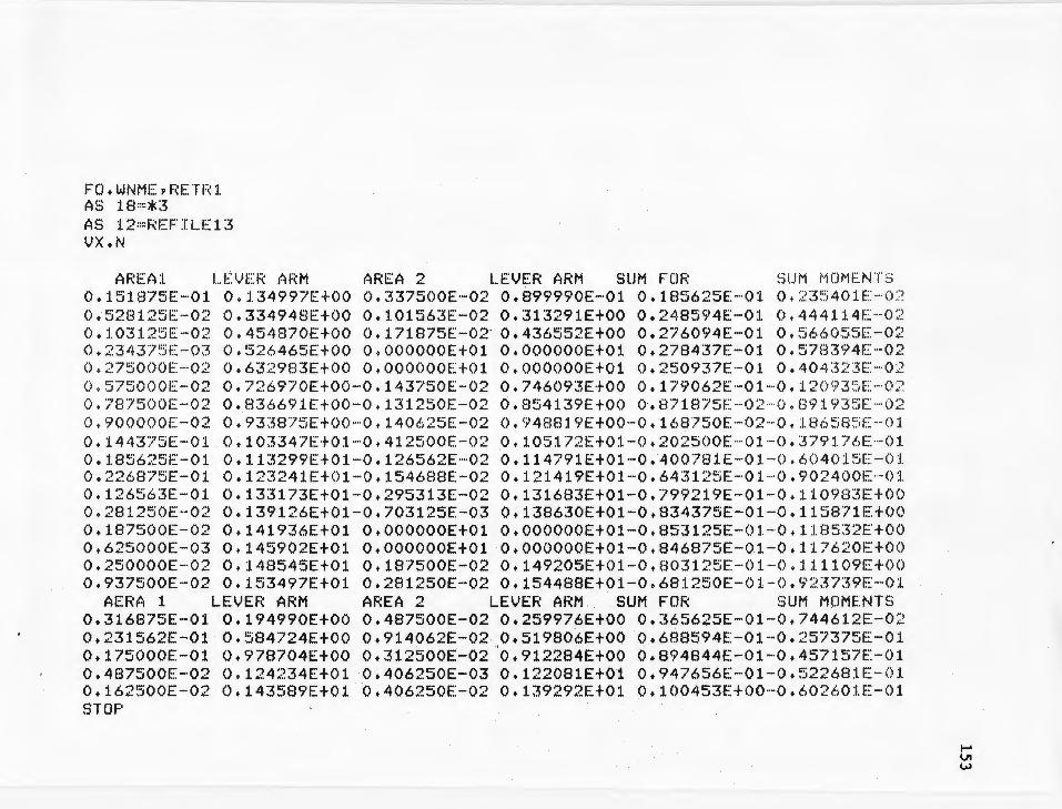
FO.WNMEYRETR1 AS 18=*3 AS 12=REFILE13 VX.N

AREA1 LEVER ARM AREA 2 LEVER ARM SUM FOR SUM MOMENT S 0.151875E-01 0.134997Et00 0.337500E-02 0.899990E-01 0.185625E-01 0.235401E-0 2 0.528125E-02 0.334948Et00 0.101563E-02 0.313291EtOO 0.248594£-01 0.444114E-02 0.103125E-02 0.454870Et00 0.171875E-02· 0.436552Et00 0.276094E-01 0.566055E-02 o.23437 5E-03 o.526465E+oo o.000000E+o1 o.000000E+o1 o.278437E-01 o.578394E - 02 o.2?soooE-02 o.632983E+oo o.000000E+o1 o.000000E+o1 o.2so937E-01 o.404323E - 02 0.575000E - 02 0.726970E+00-0.143750E-02 0.746093Et00 0.179062E-01-0.120935E - 02 0.787500E - 02 0.836691Et00- 0.131250E-02 0.854139Et00 ~.871875E-0 2-0 .891935E - 02

0.900000E-02 0.933875Et00-0.140625E-02 0.948819Et00-0.168750E-02-0.186585E-01 0.144375E-01 0.103347Et01 - 0.412500E- 02 0.105172Et01-0.202500E - 01-0.379176E-01 0.185625E-01 0.113299Et01 - 0.126562E-02 0.114791Et01-0.400781E-01 - 0.604015E-01 0.226875E-01 0.123241Et01-0.154688E-02 0.121419Et01-0.643125E-01 - 0.902400E-01 0.126563E-01 0+133173Et01-0+295313E-02 0.131683Et01-0.799219E-01-0.110983Et00 0.281250E-02 0.139126Et01-0.703125E-03 0.138630Et01-0.834375E-01-0.115871E+OO o.1s7500E-02 o.141936E+o1 o.000000E+o1 o.000000E+o1-o.as3125E-01 - o.11ss32E+oo o.625oooE-o3 o.145902E+o1 o.000000E+o1 o.000000E+o1-o.a46s75E-o1-o.117620E+oo 0.250000E-02 0.148545Et01 0.187500E-02 0.149205Et01-0.803125E-01-0.111109Et00 0.937500E-02 0.153497Et01 0.281250E-02 0.154488E+01-0.681250E-01-0.923739E- 01

AERA 1 LEVER ARM AREA 2 LEVER ARM SUM FOR SUM MOMENTS 0.316875E-01 0.194990Et00 0.487500E-02 0.259976£+00 0.365625E-01-0.744612E-02 0.231562E-01 0.584724E+oo 0+914062E-02 .0.519806Et00 0+688594E-01-0.257375E-01 0.175000E-01 o.978704E+OO 0.312500£-02 0.912284E+oo 0+894844E-01-0.457157E - 01 0.487500E-02 0.124234Et01 0.406250£-03 0.122081£+01 0.947656E-01-0+522681E-01 0.162500E-02 0.143589Et01 0.406250E-02 0.139292Et01 -0.100453Et00-0.602601E-01 STOP

!--' IJ1 (....)

FO.WNME , RETR1 AS 18=* 3 AS 12=REFILE14 vx.N

APPENDIX X

DATA FILE AND OUTPUT

{Force and moment balance)

AREA1 1...EVEF~ ARM AREA 2 LEVER ARM SUM FCm f.>LJM MOMENT ~::: 0.150937E-01 0.104998Et00 0.131250E-02 0.699995E-01 0.164062E - 01 0.1 676 69E-0 2 0.890625E- 02 0.304961Et00 0.237500E-02 0.273305Et00 0.276875E - 01 0.50 41 85E - 0? 0 .225000E- 0 2 0.444879Et00 0.984375E-03 0.429890Et00 0. 309219E - 01 0.646600E·- 0 2 o.s1soooE - 03 o.51 3 147E+oo o.000000E+o1 o.000000E+o1 o.317969 E- 01 o . 6 9 1so 1E-02 o. 250000E - 02 o.62632BE+oo o.000000E+o1 o.000000E+o1 o.292969E - 01 o.5349 19E-02 0.625000E - 02 o.721981Et00 - 0.175781E - 02 o.742768Et00 0+21 2891 E- 01 - 0.46883 8E-0 3 0.820312E-02 0.836691Et00-0.820312E- 03 0.854139Et00 0.122656E-01 - 0.803298E- 02 0.843 750E-02 0.933875Et00 - 0.154688E- 02 0.948819Et00 0 . 228125E- 0 2-0 . 173803E - 01 0.140937E-01 0.103347Et01 - 0.464062E-02 0.105172Et01 - 0.164531E-01 -0. 368 264F-0 1 0.191250E-01 0+113299Et01-0.984375E-03 0.114791Et01-0.365625E -0 1- 0.596 2 48 E - 0 1 0.233750E-01 0.123241Et01-0.120313E- 02 0+121419Et01 - 0.611406E - 01 - 0.8989 3 1E - 01 0.135000E-01 0.133173E+01-0.281250E-02 0.131683Et01-0+774531E - 01 - 0 . 1 11575EtOO 0.337500E- 02 0.139622Et01-0.~31250E-02 0.138961E+01-0.821406E-01-0+118111 F t 00

/

0. 843750j?--03 0.142267Et01 0. OOOOOOEtOl 0. OOOOOOE+Ol-0. 829B44E-·· O :I. .... (). U . 931 l E+OO o.1sooooE-02 o.145572E+o1 o.000000E+o1 o.ooooooE+o1 - o.s14s44£- 01 - o . 11 ; 12sEi ·OO 0.400000E-02 0.148545E+01 0.187500E-02 0.149205Et01-0.756094E- 01 - 0.10838 9E t0 0 0.116250E-01 -0.153497Et01 0+262500E-02 0.154488Et01 - 0.613594E-01 - 0.864892E-0 1

AERA 1 LEVER ARM AREA 2 LEVER ARM SUM FOR SUM MOMENT S 0.320625E-01 0.189991E+OO 0.356250£-02 0.253311Et00 0.356250E ·-01 ··- 0.699399E -O :~ 0.183750E-01 0.484843Et00 0.164063E~02 0.449874Et00 0.556406E- 01-0.166 411E - 01 0.118750E-01 0.684557Et00 0.237500E-02 0.652949Et00 0.698906E- 01 - 0.263209E - 0 1 0.690625E-02 0.864109Et00 0.185937E-02 o . 835860Et00 o.786562E - 01 -0 .338429E-<>1 0.934375E-02 0.106334E+01 0.359375£-03 0.110148Et01 0.883594E- 01 -0~441743E -01 0.365625£- 02 0.137142Et01 0.670313E-02 0.130691Et01 0.987187E -Ol~0 . 579489E - 0 1 STOP ......

Vt -'="'

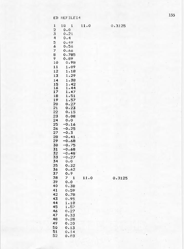
ED i:;:EF" Il...F:t. .-(.: 155

l Jn :I. U. • 0 0.3:1.2~) •"") ,\°,. () . () 3 0. 2:t -4 () .. (~ c· d (). 4 <;.>

6 (). 5f.> l ().66 8 0. 78~) 9 ().ti<;> :LO 0.9El 11 1.09 1-:> ·- l • l. 8 1.3 :L. 29 :L4 1.38 15 1.42 16 l..44 17 1.47 18 1+51 19 1.57 20 0+2'7 21 0.23 r)'") ...,, 0 .1:'.'i 23 0.08 24 o.o 25 -0.16 26 -0.25 2'7 -· O. 3 28 -0.41 29 -0.68 30 - o. n:; 31 - 0.68 32 - 0.48 33 -· O. ~-~7 34 o.o 35 0+32 36 0.62 37 0.9 38 7 l. 11 • () 0.31.25 39 (). 0 40 0. :38 41 (). ~'i9 42 O.'l!:l 43 0. 9 :'.'i 44 1.18 45 :I. • ~5 '7 46 0.27 47 0.33 48 (). 2(]

49 0.20 50 (). 1 :~ 51. (). :14 52 o. o:~

..

156

E li I ~ E F I !.. F l 0

1 :i. / :I. tl.O () ' 3 l :?. ~::;

'") (). () .. : .. 3 () + ::.l 3 4 (). 3 <,.J i::· _, 0 . ~'il

6 0. ~:i 6 7 .... . 6 !'.'j

8 0. '7B~.'i

9 (). 89 10 0.98 1.1 :I . • 07 1? ·- 1.10 L3 1.29 14 1.3B 15 1. 4 ~~

16 1.45 17 :I .• 52 18 1+57 19 0. 2 ~5

20 0.20 21 o.l3 2~~ 0. l 1 2:i (). 0 24 - 0.12 ,.) a:· A- , .1 ·-0. 24 26 --0. 28 ~!. 7 - 0.40 28 -0.56 29 -0.72 30 -0.60 31 -0.4() 32 - 0.22 33 0. () 34 o.7 35 o.94 36 7 1 :1.1. 0 0.3125 37 () . () ~rn 0.39 39 o.59 40 o. '78 41 l • 1 '7 42 :1. . 3 3 43 :t. . ~:il 44 0. 2~:S

45 0.29 46 0+ 2 4 47 (). :I. 6 48 0.:1.~~

49 (). 013 50 () . () 1

FO . WNM E ,RETR1 AS 18=*3 AS 12~REFILE10

VX+N

AREA1 LEVER ARM AREA 2 LEVER ARM SUM FOR SUM MOMENTS O.t 43750E - 01 0.11 4998Et00 0.107812E-02 0.766660E - 01 0.154531E -01 0.173575E-02 0 . 650000C - 02 0.3099 59Et00 0.175000E-02 0.283302Et00 0.237031E-01 0.424626E-02 0.412500E -02 0 . 449874EtOO 0.375000E-03 0.429890Et00 0.282031E- 01 0+626320E-·02 o.B59375E-03 o.526465E+oo o.000000E+o1 o.000000E+o1 o.290625E-01 o.671563E - 0 2 o.226B75E-01 - o.246646E+oo o.000000E+o1 o.000000E+o1 o.s17sooE-01 o.111985E-02 0.538125E-01 0.674996E-01 - 0.269062E-01 0.306627Et00-0.289688E-01-0.107626E- 01 0.787500E-02 0.836691Et00- 0.656250E - 03 0.854139Et00-0.375000E-01-0.179121E-01 0 .787500E-02 0.933875Et00- 0.168750E-02 0.948819Et00-0.470625E-01 - 0.268675E- 01 0.1 12500E- 01 0+102352Et01-0.225000E- 02 0+103845Et01-0.605625E - 01-0.407 186E-0 1 0 .192500E-01 0.112304Et01-0.275000E-02 0.114128Et01-0.825625E - 01 - 0 . 654756E-01 0.206250E-01 0.123241Et01-0.206250E-02 0+121419Et01-0.105250Et00- 0.933983E-01 0.112500E-01 0.133173Et01-0.281250E-02 0.131683Et01-0+119313Et00-0.112084EtOO 0.343750E-02 0.140118Et01-0.140625E-02 0+139292Et01-0.124156Et00-0 .11 8859Et OO 0. 6ff7!":'.iOOE -· 03 0. 143259Et01 0. 000000Et01 0. OOOOOOE+Ol-0.124844Et00-·0.119ti44Fl00 0. /65625E - 02 0. 149205Et01 0. 000000Et01 0. 000000.E+Ol-O. 117188E+OO --O . :l-08421 E+OO 0.109375E - 01 0.153993Et01 0.187500E- 02 0+154818E+01-0.104375Et00 - 0.886748E- 0 1

AERA 1 LEVER ARM AREA 2 LEVER ARM SUM FOR SUM MOMENTS 0.280312E-01 0.194990Et00 0+365625E-02 0.259976Et00 0.316875E-01 - 0.641634E-02 0.150000E-01 0.489838E+OO 0+156250E-02 0.456535Et00 0.482500E-01-0.144773E-01 0.950000E - 02 0.684557E+OO 0+237500E-02 0+652949Et00 0.601250E-01-0.225313E- 01 0.146250E-01 0.973724Et00 0+243750E- 02 0.908962Et00 0.771875Er 01-0.389876E- Oi 0.400000E-02 0.124731Et01 O.lOOOOOE-02 0+122081Ef01 0.821875E-01-0.451977E- 01 0.750000E-03 0+144580Et01 0+262500E-02 0+140614Et01 0.855625E-01-0.499731E-01 STOP

..... V1

"'

•

158

ED REFIL..E:l.2

:I. 1 ·7 :I. :l.:L • 0 o.3125 , .) (). 00 ·-3 0 r)·1

4 0 :~· · r 5 0.41 6 (). 5~7 } o.6 ·~ 8 O. lB

15

9 (). 891 10 o.~a1 11

1. r 12 1. .1 Tl :1.3 1. ~J9 14 1.J74 15 1.~3 16 1 ~"'" • 1'-' 17 1+52 18 1. ::l7 19 0 .1\5 20 o. ~4 21 o. 9 22 0.06 23 o.a 24 -ot '.. . ~ '·:

25 -0.17 26 --0 • ..-.i2

I

27 - 0.31 28

I --0·18

29 -0.55 I

30 -0.5 I

31 ·-0 r) • ,,. It ..

32 o. 33 o. ~ 2

I

34 O.q 35 O.l5 36 6 :1. 11.0 0.3125 37 o.o 38 o.38 39 0. ·79 40 l.18 41 1.49 42 1. 5·7 43 0.1.~i

44 0.2 4r.:· ··' (). 11 4c> 0.08 4/ o.o 48 ··-0. 01

FO. WNME, RETF~ 1 AS 18=*3 AS 12=REFILE12 vx.N

AREA1 LEVER ARM AREA 2 LEVER ARM SUM FOR SUM MOMENTS 0.918750E-02 0.104998Et00 0+328125E-03 0+699995E-01 0+951562E-02 0.987641E-03 0.534375E-02 0.304961Et00 0.148437E-02 0.173305Et00 0+163437E-01 0.302296E-02 0.168750E-02 0.444879E+oo 0+421875E-03 0+429890Et00 0.184531E-01 0.395506E-()2 o.s62sooE-03 o.509a17E+oo o.000000E+o1 o.000000E+o1 o.1901s6E-01 o.424183E-02 o.22soooE-02 o.629656E+oo o.000000E+o1 o.000000E+o1 o.167656E-01 o.2a2s10E-02 0.431250E-02 0.726970Et00-0.898437E-03 0.746P93Et00 0.115547E-01-0.980272E-03 o.557812E-02 0+836691E+00-0.820312E-03 0.854139E+oo 0+515625E-02-0.634810E-02 0.625625E-02 0.934373E+00-0.127969E-02 0.9494B4Et00-0.237969E-02-0.134088E-01 0.105594E-01 0.103397Et01-0.289531E-02 0.105206Et01-0.158344E-01-0.273729E- 01 0.130500E-01 0.113150Et01-0.951562E-03 0+114592Et01-0.298359E-01-0.432294E-01 0.176562E-01 0.123092Et01-0.882812E-03 0.121220Et01-0.483750E-01-0.660329E-01 0.840000E-02 0.132875Et01-0.236250E-02 o.13~485Et01-0.591375E-q1-o.ao3007E -01

o.2sooooE-02 o.138895E+o1 o.000000E+o1 o.000000E+o1-o.619375E-o1-o.a41s97f -- 01 o.375000E-03 o.143920E+o1 o.000000E+o1. o.000000E+o1-o.615625E-o1-o.e36500E-01 0.262500E-02 0.148049E+01 0.525000E-02 0+149205Et01~0.536875E-01-0.719305E-01 0.937500E-02 0.153993Et01 0.117188E-02 0+154818Et01-0+431406E-01-0.556794E- 01

AERA 1 LEVER ARM AREA 2 LEVER ARM . SUM FOR SUM MOMENTS 0.178125E-01 0.189991Et00 0.296875E-02 0.253311£+00 0.207812E-01-0.413622E-02 0.137500E-01 0.579731Et00 0+562500E-02 0.513147E+OO 0.40i562E~o1-o.149940E-01 o.100000E-01 0.978704E+OO 0+187500E-02 0+912284E+oo o;520312E~01-0.264916E~o1 o.387500E-02 o.12ao42E+o1 o.ooo-000E+o1 o.oooo-00E+o1 o.559062E-01-o.31453~E-01 o.12soooE-03 o.153827E+o1 o.000000E+o1 o.000000E+o1 o.5s7a12E-01-o.312609E-01 STOP

to-' VI \0

~

:•rr ..

APPENDIX XI

CONVERSION OF RAW DATA TO INPUT FOR COMPUTER PROGRAM

This conversion deals with data preparation pertaining to the

curve of initial residual stresses in the tube shown in ~igure 3.28.

I) Definition of areas of forces limited by the curve and the X axis.

a) The curve of initial residual stresses obtained from measured

strains in the tube with variable 4A and 4B, in Figure 3.28, has been -

drawn as follows:

-The longitudinal residual stresses computed from measured strains

for 11 holes with hole depth of 0.125", shown in Table 3.3 (column 4)

divided by yield stress, give ratios of aL/ay (colµmn 6).

-The position of each hole is located by the ratio d/r, r being the

radius of the steel tube (r = 11") and d, the distance in inch of the

hole · to the longitudinal weld, measured by cutting the tube with a

plane passing by the weld and the tube center and flattening the

cylinder on a plane parallel to the XY plane in Figure 4.8.

-On a system of perpendicular axes, plot d/r on the abscissa, crL/cry

on the ordinate. A polygonal line (see Figure A.11.1) forms the curve

which represents the pattern of distribution of longitudinal residual

stresses at each of the 11 holes drilled in the tube.

-For obtaining a better curve which may reflect the continuity of the

stresses present in the tube and give a closer value of the stress

at any hole drilled. on the semi-circular section of the 11 holes, a

continuous smooth. curved line was drawn, passing through the points

of the above polygonal line (see Figure A.11.1).

6"L. -6':f

o.s · o.s

0.4 l \\

#5

0 t , ot 19 O:-J9 '

I \\; I . -o.4

-0.75

0.34 I

B I #1 I

~14 I I I

0.59 • - - -- -- ---~-o- 2.35 2.?5 ' -- --, -- -- - - --- .u.- -~ --.-------

1.S7 •

Holef6 #2 #7 IJ rs ; /-wea--T

Figure A.11.1 Po17gonal line and CQ.(l.Ul .oontinuoua curve representing residual stres•••· Table J.11. caae 1.

).0 lt

#4

d R

..... °' .....

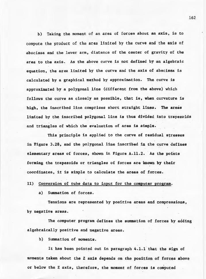
162

b) Taking the moment of an area of forces about an axis, is to

compute the product of the area limited by the curve and . the axis of

abscissa and the lever arm, distance of the center of gravity of the

area to the axis. As the above curve is not defined by an algebraic

equation, the area limited by the curve and the axis of abscissa is

calculated by a graphical me_thod by approximation. The curve is

approximated by a polygonal line (different from the above) which

follows the curve as closely as possible, that is, when curvature is

high, the inscribed line comprises short straight lines. The areas

limited by the inscribed polygonal line is thus divided into trapezoids

and triangles of which the evaluation of area is simple.

This principle is applied to the curve of residual stresses

in Figure 3.28, and the polygonal line inscribed in the curve defines

elementary areas of force_s, shown in Figure A.11. 2. As the points

forming the trapezoids or triangles of forces are known by their

coordinates, it is simple to calculate the areas of forces.

II) Conversion of tube data to input for the computer program.

a) Summation of forces.

Tensions are represented by positive areas and compressions,

by negative areas.

The computer program defines the summation of forces by adding

algebraically positive and negative areas.

b) Summation of moments.

It has been pointed out in paragraph 4.1.1 . that the sign of

moments taken about the Z axis depends on the position of forces above

or below the Z axis, therefore, the moment of forces is computed

6"1. -6"~ I 0.8

0.8

I\ .60

0.4 I 1\ .40

.19 .')9 .!f}

I

I

•' ~: ~

I 0 • J""' I I 26 ,. --- .14 .12 .... I

.16 .28 -~ .6a 0 • I : 2. 1s 2.1s ,.o x. d

. t 2.~0 J.14 -t R

-o.4 + •• 3

-0.75

~ CIQ I

. I .42

Fi&Ur! A.11.2 Pol.7&onal line inaoribed 1D oontinuou1 curT• to detl.n• el.•enta17 &!'9&8 or torces(Moaent taken about bending

a.xis. absciasa 1.57) ·

...... c:I\ w

,.

separately for forces above the Z axis and for forces below this axis.

Sample calculation. (See Figure A.11.3)

A) For areas of forces below the Z axis, abscissa 1.S7.

First trapezoid. (at right hand side of the bending axis)

Abscissa of first side, x1 (new axis) = 0.0

Abscissa of second side x2 = 1.96 - 1.S7 = 0.39

Length of first side Y1 = 0.26

Length of second side Y2 = 0.34

Second trapezoid.

Abscissa of first side, x2 = 0.39

Abscissa of second side x3 = 2. 3S - 1. S 7 = 0. 7 8

Length of first side, Y2 = 0.34

Length of second side Y3 = 0.19

Third traE_ezoid.

Abscissa of first side, x3 = 0.78

Abscissa of second side, x4 = 2.75 - 1.57 = 1.18

Length of first side, Y3

= 0.19

Length of second side, Y4 = 0.14

Fourth trapezoid.

Abscissa of first side, x4

= 1.18

Abscissa of second side XS = 2.88 - 1.57 = 1.31

Length of first side, Y4

= 0.14

Length of second side, x5

= 0.12

Fifth trapezoid.

Abscissa of first side, XS = 1.31

Abscissa of second side, x6 = 3.14 - 1.57 = 1.57

164

6"a. -6"~ . o.s

o.s I\

.60

• 19 .39

0 w

1,.16 .28

.o .1

-o.4 + -.J

-0.75

I2 = O.J4

.59 - "i.5= Y4 = .14 .12

.4& .68

.42

:r;Jr- 1 2~g 2.35 I . e9 J '· .12= .']9 j :f: X3= .78 _

2. 75 I ).0 lf. 2.tso J. ~ 4

~,~·~~=--~~~---,

i:! I 14= 1. 18 -----eot GI I ~, 15= 1.31

. ... . : 16 • 1.57 r .,

Figure A.11.J ConYarsion ot tuba data tO input tor the computer pro&raa.

I _J -i

I

d R

......

°' \JI

Length of first side, Y5 = 0.12

Length of second side, Y6

= 0.02

In Appendix IX, the input will be read as follows:

First reading. (Format statement #10)

I • number of data = 6 for this case.

J = number of set of data = 1

R = radius of the tube = 11.0 (inches)

T a thickness of the tube = 0.3125 (inches)

(see Appendix IX B, line 38)

Second reading. (Format statement 1120)

X(N), by turns, equals

x1 = o.o, x1 = o.34, x3 s o.78, x4 = 1.18, x5

- 1.31, x6

- 1.57

(see Appendix IX B. lines 38 to 44)

Third reading. (Format statement #40)

Y(N), by turns, equals

Y1 = 0.26, Y2 = o.34, Y3 = 0.19, Y4 = 0.14, Y5

- 0.12, Y6

- 0.02

(see Appendix IX b, lines 45 to 50)

B) For areas of forces above the Z axis.

166

The same approach will lead to the input presented in Appendix

IX B, line 1 to line 37.