an experimental comparison of min-cut/max-flow …vnk/papers/bk-pami04.pdf · an experimental...

IEEE Transactions on PAMI (TPAMI-0120-0603) first submitted in May, 2002 p.1

An Experimental Comparison ofMin-Cut/Max-Flow Algorithms for

Energy Minimization in Vision

Yuri Boykov and Vladimir Kolmogorov∗

Abstract

After [15, 31, 19, 8, 25, 5] minimum cut/maximum flow algorithms on graphs emerged as

an increasingly useful tool for exact or approximate energy minimization in low-level vision.

The combinatorial optimization literature provides many min-cut/max-flow algorithms with

different polynomial time complexity. Their practical efficiency, however, has to date been

studied mainly outside the scope of computer vision. The goal of this paper is to provide an

experimental comparison of the efficiency of min-cut/max flow algorithms for applications

in vision. We compare the running times of several standard algorithms, as well as a

new algorithm that we have recently developed. The algorithms we study include both

Goldberg-Tarjan style “push-relabel” methods and algorithms based on Ford-Fulkerson

style “augmenting paths”. We benchmark these algorithms on a number of typical graphs

in the contexts of image restoration, stereo, and segmentation. In many cases our new

algorithm works several times faster than any of the other methods making near real-time

performance possible. An implementation of our max-flow/min-cut algorithm is available

upon request for research purposes.

Index Terms — Energy minimization, graph algorithms, minimum cut, maximum

flow, image restoration, segmentation, stereo, multi-camera scene reconstruction.

∗Yuri Boykov is with the Computer Science Department at the University of Western Ontario, Canada,[email protected]. Vladimir Kolmogorov is with Microsoft Research, Cambridge, England, [email protected] work was mainly done while the authors were with Siemens Corp. Research, Princeton, NJ.


1 Introduction

Greig et al. [15] were first to discover that powerful min-cut/max-flow algorithms from combi-

natorial optimization can be used to minimize certain important energy functions in vision. The

energies addressed by Greig et al. and by most later graph-based methods (e.g. [32, 18, 4, 17, 8,

2, 30, 39, 21, 36, 38, 6, 23, 24, 9, 26]) can be represented as1

E(L) =∑

p∈P

Dp(Lp) +∑

(p,q)∈N

Vp,q(Lp, Lq), (1)

where L = {Lp |p ∈ P} is a labeling of image P, Dp(·) is a data penalty function, Vp,q is

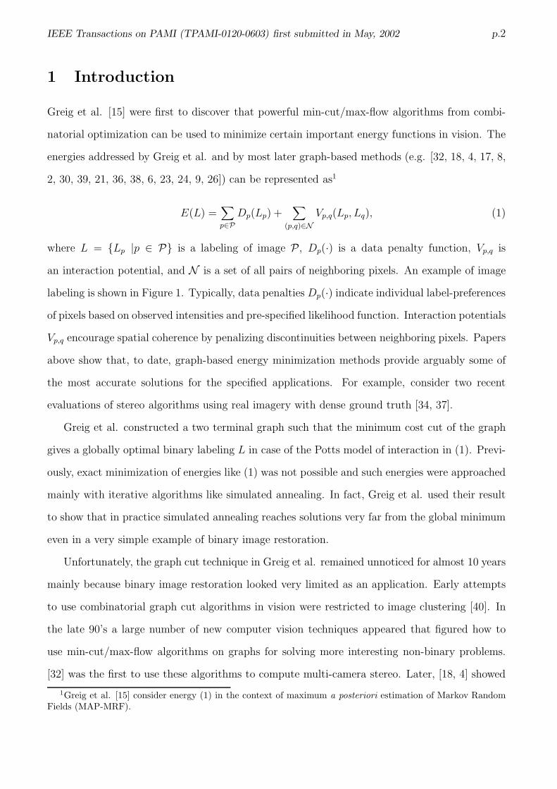
an interaction potential, and N is a set of all pairs of neighboring pixels. An example of image

labeling is shown in Figure 1. Typically, data penalties Dp(·) indicate individual label-preferences

of pixels based on observed intensities and pre-specified likelihood function. Interaction potentials

Vp,q encourage spatial coherence by penalizing discontinuities between neighboring pixels. Papers

above show that, to date, graph-based energy minimization methods provide arguably some of

the most accurate solutions for the specified applications. For example, consider two recent

evaluations of stereo algorithms using real imagery with dense ground truth [34, 37].

Greig et al. constructed a two terminal graph such that the minimum cost cut of the graph

gives a globally optimal binary labeling L in case of the Potts model of interaction in (1). Previ-

ously, exact minimization of energies like (1) was not possible and such energies were approached

mainly with iterative algorithms like simulated annealing. In fact, Greig et al. used their result

to show that in practice simulated annealing reaches solutions very far from the global minimum

even in a very simple example of binary image restoration.

Unfortunately, the graph cut technique in Greig et al. remained unnoticed for almost 10 years

mainly because binary image restoration looked very limited as an application. Early attempts

to use combinatorial graph cut algorithms in vision were restricted to image clustering [40]. In

the late 90’s a large number of new computer vision techniques appeared that figured how to

use min-cut/max-flow algorithms on graphs for solving more interesting non-binary problems.

[32] was the first to use these algorithms to compute multi-camera stereo. Later, [18, 4] showed

1Greig et al. [15] consider energy (1) in the context of maximum a posteriori estimation of Markov RandomFields (MAP-MRF).


2

2

2

2

2 2

2222

1

0 1

0

1

0

1

0

1

0

1

0

1

0

1

0

1

0

1

0

1

0

1

0

1

0

1

1

1 1

11

(a) An image (b) A labeling

Figure 1: An example of image labeling. An image in (a) is a set of pixels P with observed

intensities Ip for each p ∈ P. A labeling L shown in (b) assigns some label Lp ∈ {0, 1, 2} to

each pixel p ∈ P. Such labels can represent depth (in stereo), object index (in segmentation),

original intensity (in image restoration), or other pixel properties. Normally, graph-based meth-

ods assume that a set of feasible labels at each pixel is finite. Thick lines in (b) show labeling

discontinuities between neighboring pixels.

that with the right edge weights on a graph similar to that used in [32] one can minimize a

fairly general energy function (1) in a multi-label case with linear interaction penalties. This

graph construction was further generalized to handle arbitrary convex cliques in [19]. Another

general case of multi-label energies where interaction penalty is a metric (on the space of labels)

was studied in [4, 8]. Their α-expansion algorithm finds provably good approximate solutions

by iteratively running min-cut/max-flow algorithms on appropriate graphs. The case of metric

interactions includes many kinds of “robust” cliques that are frequently preferred in practice.

Several recent papers studied theoretical properties of graph constructions used in vision.

The question of what energy functions can be minimized via graph cuts was addressed in [25].

This work provided a simple necessary and sufficient condition on such functions. However, the

results in [25] apply only to energy functions of binary variables with double and triple cliques.

In fact, full potential of graph-cut techniques in multi-label cases is still not entirely understood.

Geometric properties of segments produced by graph-cut methods were investigated in [3].

This work studied cut metric on regular grid-graphs and showed that discrete topology of graph-

cuts can approximate any continuous Riemannian metric space. The results in [3] established a

link between two standard energy minimization approaches frequently used in vision: combina-

torial graph-cut methods and geometric methods based on level-sets (e.g. [35, 29, 33, 28]).


A growing number of publications in vision use graph-based energy minimization techniques

for applications like image segmentation [18, 39, 21, 5], restoration [15], stereo [32, 4, 17, 23, 24, 9],

shape reconstruction [36], object recognition [2], augmented reality [38], texture synthesis [26],

and others. The graphs corresponding to these applications are usually huge 2D or 3D grids,

and min-cut/max-flow algorithm efficiency is an issue that cannot be ignored.

The main goal of this paper is to compare experimentally the running time of several min-

cut/max-flow algorithms on graphs typical for applications in vision. In Section 2 we provide

basic facts about graphs, min-cut and max-flow problems, and some standard combinatorial

optimization algorithms for them. We consider both Goldberg-Tarjan style push-relabel algo-

rithms [14] as well as methods based on augmenting paths a la Ford-Fulkerson [13]. Note that

in the course of our experiments with standard augmenting path techniques we developed some

new algorithmic ideas that significantly boosted empirical performance on grid-graphs in vi-

sion. Section 3 describes our new min-cut/max-flow algorithm. In Section 4 we tested this new

augmenting-path style algorithm as well as three standard algorithms: the H PRF and Q PRF

versions of the “push-relabel” method [14, 10], and the Dinic algorithm [12] that also uses aug-

menting paths. We selected several examples in image restoration, stereo, and segmentation

where different forms of energy (1) are minimized via graph structures originally described in

[15, 18, 4, 8, 23, 24, 6]. Such (or very similar) graphs are used in all computer vision papers known

to us that use graph cut algorithms. In many interesting cases our new algorithm was signifi-

cantly faster than the standard min-cut/max-flow techniques from combinatorial optimization.

More detailed conclusions are presented in Section 5.

2 Background on Graphs

In this section we review some basic facts about graphs in the context of energy minimization

methods in vision. A directed weighted (capacitated) graph G = 〈V, E〉 consists of a set of nodes

V and a set of directed edges E that connect them. Usually the nodes correspond to pixels,

voxels, or other features. A graph normally contains some additional special nodes that are

called terminals. In the context of vision, terminals correspond to the set of labels that can

be assigned to pixels. We will concentrate on the case of graphs with two terminals. Then


sink

source

qp

s

t

source

sink

cut

qp

s

t

(a) A graph G (b) A cut on G

Figure 2: Example of a directed capacitated graph. Edge costs are reflected by their thickness.

A similar graph-cut construction was first used in vision by Greig et al. [15] for binary image

restoration.

the terminals are usually called the source, s, and the sink, t. In Figure 2(a) we show a simple

example of a two terminal graph (due to Greig et al. [15]) that can be used to minimize the Potts

case of energy (1) on a 3 × 3 image with two labels. There is some variation in the structure of

graphs used in other energy minimization methods in vision. However, most of them are based

on regular 2D or 3D grid graphs as the one in Figure 2(a). This is a simple consequence of the

fact that normally graph nodes represent regular image pixels or voxels.

All edges in the graph are assigned some weight or cost. A cost of a directed edge (p, q) may

differ from the cost of the reverse edge (q, p). In fact, ability to assign different edge weights for

(p, q) and (q, p) is important for many graph-based applications in vision. Normally, there are

two types of edges in the graph: n-links and t-links. N-links connect pairs of neighboring pixels

or voxels. Thus, they represent a neighborhood system in the image. Cost of n-links corresponds

to a penalty for discontinuity between the pixels. These costs are usually derived from the pixel

interaction term Vp,q in energy (1). T-links connect pixels with terminals (labels). The cost of a

t-link connecting a pixel and a terminal corresponds to a penalty for assigning the corresponding

label to the pixel. This cost is normally derived from the data term Dp in the energy (1).

2.1 Min-Cut and Max-Flow Problems

An s/t cut C on a graph with two terminals is a partitioning of the nodes in the graph into two

disjoint subsets S and T such that the source s is in S and the sink t is in T . For simplicity,

throughout this paper we refer to s/t cuts as just cuts. Figure 2(b) shows one example of a cut.


Original image (a) A maximum flow (b) A minimum cut

Figure 3: Graph cut/flow example in the context of image segmentation in Section 4.4. Red and

blue seeds are “hard-wired” to the source s and the sink t, correspondingly. As usual, the cost of

edges between the pixels (graph nodes) is set to low values in places with high intensity contrast.

Thus, cuts along object boundaries in the image should be cheaper. Weak edges also work as

“bottlenecks” for a flow. In (a) we show a maximum flow from s to t. In fact, it saturates graph

edges corresponding to a minimum cut boundary in (b).

In combinatorial optimization the cost of a cut C = {S, T } is defined as the sum of the costs of

“boundary” edges (p, q) where p ∈ S and q ∈ T . Note that cut cost is “directed” as it sums up

weights of directed edges specifically from S to T . The minimum cut problem on a graph is to

find a cut that has the minimum cost among all cuts.

One of the fundamental results in combinatorial optimization is that the minimum s/t cut

problem can be solved by finding a maximum flow from the source s to the sink t. Loosely

speaking, maximum flow is the maximum “amount of water” that can be sent from the source to

the sink by interpreting graph edges as directed “pipes” with capacities equal to edge weights.

The theorem of Ford and Fulkerson [13] states that a maximum flow from s to t saturates a

set of edges in the graph dividing the nodes into two disjoint parts {S, T } corresponding to a

minimum cut. Thus, min-cut and max-flow problems are equivalent. In fact, the maximum

flow value is equal to the cost of the minimum cut. “Duality” relationship between maximum

flow and minimum cut problems is illustrated in Fig. 3 in the context of image segmentation.

Max-flow displayed in Fig. 3(a) saturates the edges in the min-cut boundary in Fig. 3(b).

We can intuitively show how min-cut (or max-flow) on a graph may help with energy min-

imization over image labelings. Consider an example in Figure 2. The graph corresponds to

a 3 × 3 image. Any s/t cut partitions the nodes into disjoint groups each containing exactly


one terminal. Therefore, any cut corresponds to some assignment of pixels (nodes) to labels

(terminals). If edge weights are appropriately set based on parameters of an energy, a minimum

cost cut will correspond to a labeling with the minimum value of this energy.2

2.2 Standard Algorithms in Combinatorial Optimization

An important fact in combinatorial optimization is that there are polynomial algorithms for min-

cut/max-flow problems on directed weighted graphs with two terminals. Most of the algorithms

belong to one of the following two groups: Goldberg-Tarjan style “push-relabel” methods [14]

and algorithms based on Ford-Fulkerson style “augmenting paths” [13].

Standard augmenting paths based algorithms, such as Dinic algorithm [12], work by pushing

flow along non-saturated paths from the source to the sink until the maximum flow in the graph

G is reached. A typical augmenting path algorithm stores information about the distribution

of the current s → t flow f among the edges of G using a residual graph Gf . The topology

of Gf is identical to G but capacity of an edge in Gf reflects the residual capacity of the same

edge in G given the amount of flow already in the edge. At the initialization there is no flow

from the source to the sink (f=0) and edge capacities in the residual graph G0 are equal to the

original capacities in G. At each new iteration the algorithm finds the shortest s → t path along

non-saturated edges of the residual graph. If a path is found then the algorithm augments it by

pushing the maximum possible flow df that saturates at least one of the edges in the path. The

residual capacities of edges in the path are reduced by df while the residual capacities of the

reverse edges are increased by df . Each augmentation increases the total flow from the source

to the sink f = f + df . The maximum flow is reached when any s → t path crosses at least one

saturated edge in the residual graph Gf .

Dinic algorithm uses breadth-first search to find the shortest paths from s to t on the residual

graph Gf . After all shortest paths of a fixed length k are saturated, the algorithm starts the

breadth-first search for s → t paths of length k + 1 from scratch. Note that the use of shortest

paths is an important factor that improves theoretical running time complexities for algorithms

2Different graph-based energy minimization methods may use different graph constructions, as well as, differentrules for converting graph cuts into image labelings. Details for each method are described in the originalpublications.


based on augmenting paths. The worst case running time complexity for Dinic algorithm is

O(mn2) where n is the number of nodes and m is the number of edges in the graph.

Push-relabel algorithms [14] use quite a different approach. They do not maintain a valid

flow during the operation; there are “active” nodes that have a positive “flow excess”. Instead,

the algorithms maintain a labeling of nodes giving a low bound estimate on the distance to

the sink along non-saturated edges. The algorithms attempt to “push” excess flows towards

nodes with smaller estimated distance to the sink. Typically, the “push” operation is applied to

active nodes with the largest distance (label) or based on FIFO selection strategy. The distances

(labels) progressively increase as edges are saturated by push operations. Undeliverable flows

are eventually drained back to the source. We recommend our favorite text-book on basic graph

theory and algorithms [11] for more details on push-relabel and augmenting path methods.

Note that the most interesting applications of graph cuts to vision use directed N-D grids

with locally connected nodes. It is also typical that a large portion of the nodes is connected

to the terminals. Unfortunately, these conditions rule out many specialized min-cut/max-flow

algorithms that are designed for some restricted classes of graphs. Examples of interesting but

inapplicable methods include randomized techniques for dense undirected graphs [20], methods

for planar graphs assuming small number of terminal connections [27, 16], and others.

3 New Min-Cut/Max-Flow Algorithm

In this section we present a new algorithm developed during our attempts to improve empirical

performance of standard augmenting path techniques on graphs in vision. Normally, see Sec-

tion 2.2, augmenting path based methods start a new breadth-first search for s → t paths as soon

as all paths of a given length are exhausted. In the context of graphs in computer vision, building

a breadth-first search tree typically involves scanning the majority of image pixels. Practically

speaking, it could be a very expensive operation if it has to be performed too often. Indeed, our

real-data experiments in vision confirmed that rebuilding a search tree on graphs makes stan-

dard augmenting path techniques perform poorly in practice. We developed several ideas that

improved empirical performance of augmenting path techniques on graphs in computer vision.

The new min-cut/max-flow algorithm presented here belongs to the group of algorithms based


A

A

A A

A

PA

A

P

P

P

P

P

P

P

P

P P

P P

P

PP

P

s t

P A A P

A

Figure 4: Example of the search trees S (red nodes) and T (blue nodes) at the end of the growth

stage when a path (yellow line) from the source s to the sink t is found. Active and passive nodes

are labeled by letters A and P, correspondingly. Free nodes appear in black.

on augmenting paths. Similarly to Dinic [12] it builds search trees for detecting augmenting

paths. In fact, we build two search trees, one from the source and the other from the sink3.

The other difference is that we reuse these trees and never start building them from scratch.

The drawback of our approach is that the augmenting paths found are not necessarily shortest

augmenting path; thus the time complexity of the shortest augmenting path is no longer valid.

The trivial upper bound on the number of augmentations for our algorithm is the cost of the

minimum cut |C|, which results in the worst case complexity O(mn2|C|). Theoretically speaking,

this is worse than complexities of the standard algorithms discussed in Section 2.2. However,

experimental comparison in Section 4 shows that on typical problem instances in vision our

algorithm significantly outperforms standard algorithms.

3.1 Algorithm’s Overview

Figure 4 illustrates our basic terminology. We maintain two non-overlapping search trees S and

T with roots at the source s and the sink t, correspondingly. In tree S all edges from each parent

node to its children are non-saturated, while in tree T edges from children to their parents are

non-saturated. The nodes that are not in S or T are called “free”. We have

S ⊂ V, s ∈ S, T ⊂ V, t ∈ T, S ∩ T = ∅.3Note that in the earlier publication [7] we used a single tree rooted at the source that searched for the sink.

The two-trees version presented here treats the terminals symmetrically. Experimentally, the new algorithmconsistently outperforms the one in [7].


The nodes in the search trees S and T can be either “active” or “passive”. The active nodes

represent the outer border in each tree while the passive nodes are internal. The point is that

active nodes allow trees to “grow” by acquiring new children (along non-saturated edges) from a

set of free nodes. The passive nodes can not grow as they are completely blocked by other nodes

from the same tree. It is also important that active nodes may come in contact with the nodes

from the other tree. An augmenting path is found as soon as an active node in one of the trees

detects a neighboring node that belongs to the other tree.

The algorithm iteratively repeats the following three stages:

• “growth” stage: search trees S and T grow until they touch giving an s → t path

• “augmentation” stage: the found path is augmented, search tree(s) break into forest(s)

• “adoption” stage: trees S and T are restored.

At the growth stage the search trees expand. The active nodes explore adjacent non-saturated

edges and acquire new children from a set of free nodes. The newly acquired nodes become

active members of the corresponding search trees. As soon as all neighbors of a given active

node are explored the active node becomes passive. The growth stage terminates if an active

node encounters a neighboring node that belongs to the opposite tree. In this case we detect a

path from the source to the sink, as shown in Figure 4.

The augmentation stage augments the path found at the growth stage. Since we push through

the largest flow possible some edge(s) in the path become saturated. Thus, some of the nodes in

the trees S and T may become “orphans”, that is, the edges linking them to their parents are

no longer valid (they are saturated). In fact, the augmentation phase may split the search trees

S and T into forests. The source s and the sink t are still roots of two of the trees while orphans

form roots of all other trees.

The goal of the adoption stage is to restore single-tree structure of sets S and T with roots

in the source and the sink. At this stage we try to find a new valid parent for each orphan.

A new parent should belong to the same set, S or T , as the orphan. A parent should also be

connected through a non-saturated edge. If there is no qualifying parent we remove the orphan

from S or T and make it a free node. We also declare all its former children as orphans. The


stage terminates when no orphans are left and, thus, the search tree structures of S and T are

restored. Since some orphan nodes in S and T may become free the adoption stage results in

contraction of these sets.

After the adoption stage is completed the algorithm returns to the growth stage. The algo-

rithm terminates when the search trees S and T can not grow (no active nodes) and the trees are

separated by saturated edges. This implies that a maximum flow is achieved. The corresponding

minimum cut can be determined by S = S and T = T .

3.2 Details of Implementation

Assume that we have a directed graph G = 〈V, E〉. As for any augmenting path algorithm, we

will maintain a flow f and the residual graph Gf (see Section 2.2). We will keep the lists of all

active nodes, A, and all orphans, O. The general structure of the algorithm is:

initialize: S = {s}, T = {t}, A = {s, t}, O = ∅while true

grow S or T to find an augmenting path P from s to t

if P = ∅ terminate

augment on P

adopt orphans

end while

The details of the growth, augmentation, and adoption stages are described below. It is convenient

to store content of search trees S and T via flags TREE(p) indicating affiliation of each node p

so that

TREE(p) =

S if p ∈ ST if p ∈ T∅ if p isfree

If node p belongs to one of the search trees then the information about its parent will be stored

as PARENT (p). Roots of the search trees (the source and the sink), orphans, and all free nodes

have no parents, t.e. PARENT (p) = ∅. We will also use notation tree cap(p → q) to describe

residual capacity of either edge (p, q) if TREE(p) = S or edge (q, p) if TREE(p) = T . These

edges should be non-saturated in order for node p to be a valid parent of its child q depending

on the search tree.


3.2.1 Growth stage:

At this stage active nodes acquire new children from a set of free nodes.

while A 6= ∅pick an active node p ∈ A

for every neighbor q such that tree cap(p → q) > 0

if TREE(q) = ∅ then add q to search tree as an active node:

TREE(q) := TREE(p), PARENT (q) := p, A := A ∪ {q}if TREE(q) 6= ∅ and TREE(q) 6= TREE(p) return P = PATHs→t

end for

remove p from A

end while

return P = ∅

3.2.2 Augmentation stage:

The input for this stage is a path P from s to t. Note that the orphan set is empty in the

beginning of the stage, but there might be some orphans in the end since at least one edge in P

becomes saturated.

find the bottleneck capacity ∆ on P

update the residual graph by pushing flow ∆ through P

for each edge (p, q) in P that becomes saturated

if TREE(p) = TREE(q) = S then set PARENT (q) := ∅ and O := O ∪ {q}if TREE(p) = TREE(q) = T then set PARENT (p) := ∅ and O := O ∪ {p}

end for

3.2.3 Adoption stage:

During this stage all orphan nodes in O are processed until O becomes empty. Each node p

being processed tries to find a new valid parent within the same search tree; in case of success p

remains in the tree but with a new parent, otherwise it becomes a free node and all its children

are added to O.

while O 6= ∅


pick an orphan node p ∈ O and remove it from O

process p

end while

The operation “process p” consists of the following steps. First we are trying to find a new

valid parent for p among its neighbors. A valid parent q should satisfy: TREE(q) = TREE(p),

tree cap(q → p) > 0, and the “origin” of q should be either source or sink. Note that the last

condition is necessary because during adoption stage some of the nodes in the search trees S or

T may originate from orphans.

If node p finds a new valid parent q then we set PARENT (p) = q. In this case p remains

in its search tree and the active (or passive) status of p remains unchanged. If p does not find a

valid parent then p becomes a free node and the following operations are performed:

• scan all neighbors q of p such that TREE(q) = TREE(p):

– if tree cap(q → p) > 0 add q to the active set A

– if PARENT (q) = p add q to the set of orphans O and set PARENT (q) := ∅

• TREE(p) := ∅, A := A − {p}

Note that as p becomes free all its neighbors connected through non-saturated edges should

became active. It may happen that some neighbor q did not qualify as a valid parent during

adoption stage because it did not originate from the source or the sink. However, this node could

be a valid parent after adoption stage is finished. At this point q must have active status as it is

located next to a free node p.

3.3 Algorithm tuning

The proof of correctness of the algorithm presented above is straightforward (see [22]). At the

same time, our description leaves many free choices in implementing certain details. For example,

we found that the order of processing active nodes and orphans may have a significant effect on

the algorithm’s running time. Our preferred processing method is a minor variation of “First-

In-First-Out”. In this case the growth stage can be described as a breadth-first search. This

guarantees that at least the first path from the source to the sink is the shortest. Note that


the search tree may change unpredictably during adoption stage. Thus, we can not guarantee

anything about paths found after the first one.

There are several additional free choices in implementing the adoption stage. For example,

as an orphan looks for a new parent it has to make sure that a given candidate is connected

to the source or to the sink. We found that “marking” nodes confirmed to be connected to the

source at a given adoption stage helps to speed up the algorithm. In this case other orphans

do not have to trace the roots of their potential parents all the way to the terminals. We also

found that keeping distance-to-source information in addition to these “marks” allows orphans

to select new parents that are closer to the source. This further helps with the algorithm’s speed

because we get shorter paths.

We used a fixed tuning of our algorithm in all experiments of Section 4. Complete details of

this tuning can be found in [22]. A library with our implementation is available upon request for

research purposes. The general goal of tuning was to make augmenting paths as short as possible.

Note that augmenting paths on graphs in vision can be easily visualized. In the majority of cases

such graphs are regular grids of nodes that correspond to image pixels. Then, augmenting paths

and the whole graph flow can be meaningfully displayed (e.g. Figure 3(a)). We can also display

the search trees at different stages. This allows a very intuitive way of tuning max-flow methods

in vision.

4 Experimental Tests on Applications in Vision

In this section we experimentally test min-cut/max-flow algorithms for three different appli-

cations in computer vision: image restoration (Section 4.2), stereo (Section 4.3), and object

segmentation (Section 4.4). We chose formulations where certain appropriate versions of energy

(1) can be minimized via graph cuts. The corresponding graph structures were previously de-

scribed by [15, 18, 4, 8, 23, 24, 5] in detail. These (or very similar) structures are used in all

computer vision applications with graph cuts (that we are aware of) to date.


4.1 Experimental Setup

Note that we could not test all known min-cut/max-flow algorithms. In our experimental tests on

graph-based energy minimization methods in vision we compared the new algorithm in Section 3

and the following standard min-cut/max-flow algorithms outlined in Section 2.2:

DINIC: Algorithm of Dinic [12].

H PRF: Push-Relabel algorithm [14] with the highest level selection rule.

Q PRF: Push-Relabel algorithm [14] with the queue based selection rule.

Many previous experimental tests, including the results in [10], show that the last two algorithms

work consistently better than a large number of other min-cut/max-flow algorithms of combina-

torial optimization. The theoretical worst case complexities for these “push-relabel” algorithms

are O(n3) for Q PRF and O(n2√

m) for H PRF.

For DINIC, H PRF, and Q PRF we used the implementations written by Cherkassky and

Goldberg [10], except that we converted them from C to C++ style and modified the interface (i.e.

functions for creating a graph). Both H PRF and Q PRF use global and gap relabeling heuristics.

Our algorithm was implemented in C++. We selected a tuning described in Section 3.3 with

more details available in [22]. We did not make any machine specific optimization (such as

pipeline-friendly instruction scheduling or cache-friendly memory usage).

Experiments in sections 4.2 and 4.4 were performed on 1.4GHz Pentium IV PC (2GB RAM,

8KB L1 cache, 256KB L2 cache), and experiments in Section 4.3 were performed on UltraSPARC

II workstation with four 450 MHz processors and 4GB RAM. In the former case we used Microsoft

Visual C++ 6.0 compiler, Windows NT platform and in the latter case - GNU C++ compiler,

version 3.2.2 with the flag “-O5”, SunOS 5.8 platform. To get system time, we used ftime()

function in Unix and ftime() function in Windows. Although these functions do not measure

process computation time, we felt that they were appropriate since we got very consistent results

(within 1%) when running tests multiple times.


(a) Diamond restoration (b) Original Bell Quad (c)“Restored” Bell Quad

Figure 5: Image Restoration Examples

4.2 Image Restoration

Image restoration is a representative early vision problem. The goal is to restore original pixel

intensities from the observed noisy data. Some examples of image restoration are shown in

Figure 5. The problem can be very easily formulated in terms of energy (1) minimization. In

fact, many other low level vision problems can be represented by the same energies. We chose

the context of image restoration mainly for its simplicity.

In this section we consider two examples of energy (1) based on the Potts and linear models

of interaction, correspondingly. Besides image restoration [15], graph methods for minimizing

Potts energy were used in segmentation [21], stereo [4, 8], object recognition [2], shape recon-

struction [36], and augmented reality [38]. Linear interaction energies were used in stereo [32]

and segmentation [18]. Minimization of the linear interaction energy is based on graphs that

are quite different from what is used for the Potts model. At the same time, there is very little

variation between the graphs in different applications when the same type of energy is used.

They mainly differ in their specific edge cost settings while the topological properties of graphs

are almost identical once the energy model is fixed.

4.2.1 Potts Model

The Potts energy that we use for image restoration is

E(I) =∑

p∈P

||Ip − Iop || +

∑

(p,q)∈N

K(p,q) · T (Ip 6= Iq) (2)


where I = {Ip |p ∈ P} is a vector of unknown “true” intensities of pixels in image P and

Io = {Iop |p ∈ P} are observed intensities corrupted by noise. The Potts interactions are specified

by penalties K(p,q) for intensity discontinuities between neighboring pixels. Function T (·) is 1

if the condition inside parenthesis is true and 0 otherwise. In the case of two labels the Potts

energy can be minimized exactly using the graph cut method of Greig et al. [15].

We consider image restoration with multiple labels where the problem becomes NP hard. We

use iterative α-expansion method in [8] which is guaranteed to find a solution within a factor

of two from the global minimum of the Potts energy. At a given iteration [8] allows any subset

of pixels to switch to a fixed label α. In fact, the algorithm finds an optimal subset of pixels

that gives the largest decrease in the energy. The computation is done via graph cuts using

some generalization of the basic graph structure in [15] (see Figure 2). The algorithm repeatedly

cycles through all possible labels α until no further improvement is possible.

Two tables below present the running times (in seconds, 1.4GHz Pentium IV) when different

max-flow/min-cut algorithms are employed in the basic step of each α-expansion. Each table

corresponds to one of the original images shown in Figure 5. The number of allowed labels is 210

(Diamond) and 244 (Bell Quad), correspondingly. We run the algorithms on images at different

resolutions. At each column we state the exact size (HxW) in pixels. Note that the total number

of pixels increases by a factor of 2 from left to right. See Figure 6 for logarithmic scale plots.

method

DINICH PRFQ PRFOur

input: Diamond, 210 labels35x35 50x50 70x70 100x100 141x141 200x200 282x282

0.39 0.77 3.42 4.19 13.85 43.00 136.760.17 0.34 1.16 1.68 4.69 12.97 32.740.16 0.35 1.24 1.70 5.14 14.09 40.830.16 0.20 0.71 0.74 2.21 4.49 12.14

method

DINICH PRFQ PRFOur

input: Bell Quad, 244 labels44x44 62x62 87x87 125x125 176x176 250x250

1.32 4.97 13.49 37.81 101.39 259.190.31 0.72 1.72 3.85 8.24 18.690.20 1.00 1.70 4.31 10.65 25.040.19 0.48 0.98 2.11 4.84 10.47

Note that the running times above correspond to the end of the first cycle of the α-expansion

method in [8] when all labels were expanded once. The relative speeds of different max-flow/min-

cut algorithms do not change much when the energy minimization is run to convergence. The


(a) Diamond, 210 labels (b) Bell Quad, 244 labels

Figure 6: Running times for the α-expansion algorithm [8]. The results are obtained in thecontext of image restoration with the Potts model (see Section 4.2.1). In two examples (a) and(b) we fixed the number of allowed labels but varied image size in order to estimate empiricalcomplexities of tested min-cut/max-flow algorithms. Images of smaller size were obtained bysubsampling. Our running time plots are presented in logarithmic scale. Note that empiricalcomplexities of each algorithm can be estimated from slopes of each plot. Dashed-lines providereference slopes for linear and quadratic growth. All max-flow/min-cut algorithms gave near-linear (with respect to image size) performance in these experiments.

number of cycles it takes to converge can vary from 1 to 3 for different resolutions/images. Thus,

the running times to convergence are hard to compare between the columns and we do not

present them. In fact, restoration results are quite good even after the first iteration. In most

cases additional iterations do not improve the actual output much. Figure 5(a) shows the result

of the Potts model restoration of the Diamond image (100x100) after the first cycle of iterations.

4.2.2 Linear interaction energy

Here we consider image restoration with “linear” interaction energy. Figure 5(c) shows one

restoration result that we obtained in our experiments with this energy. The linear interaction

energy can be written as

E(I) =∑

p∈P

||Ip − Iop || +

∑

(p,q)∈N

A(p,q) · |Ip − Iq| (3)


where constants A(p,q) describe the relative importance of interactions between neighboring pixels

p and q. If the set of labels is finite and ordered then this energy can be minimized exactly using

either of the two almost identical graph-based methods developed in [18, 4]. In fact, these

methods use graphs that are very similar to the one introduced by [32, 31] in the context of

multi-camera stereo. The graphs are constructed by consecutively connecting multiple layers of

image-grids. Each layer corresponds to one label. The two terminals are connected only to the

first and the last layers. Note that the topological structure of these graphs is noticeably different

from the Potts model graphs especially when the number of labels (layers) is large.

The tables below show the running times (in seconds on 1.4GHz, Pentium IV) that different

min-cut/max-flow algorithms took to compute the exact minimum of the linear interactions

energy (3). We used the same Diamond and Bell Quad images as in the Potts energy tests. We

run the algorithms on images at different resolution. At each column we state the exact size

(hight and width) in pixels. Note that the total number of pixels increases by a factor of 2 from

left to right. Also, see Figure 7 (a,b) for logarithmic scale plots.

method

DINICH PRFQ PRFOur

input: Diamond, 54 labels35x35 50x50 70x70 100x100 141x141 200x200

1.34 4.13 8.86 18.25 34.84 57.090.47 1.30 3.03 7.48 17.53 43.580.55 1.16 3.05 6.50 12.77 22.480.17 0.33 0.63 1.41 2.88 5.98

method

DINICH PRFQ PRFOur

input: Bell Quad, 32 labels44x44 62x62 87x87 125x125 176x176 250x250

0.55 1.25 2.77 6.89 15.69 31.910.48 1.25 2.75 7.42 17.69 38.810.27 0.56 1.55 2.39 6.78 10.360.13 0.27 0.52 1.09 2.33 4.84

The structure of linear interaction graph directly depends on the number of labels4. In fact,

if there are only two labels then the graph is identical to the Potts model graph. However, both

size and topological properties of the linear interaction graphs change as the number of labels

(layers) gets larger and larger. Below we compare the running times of the algorithms for various

numbers of allowed labels (layers). We consider the same two images, Diamond and Bell Quad.

4Note that in Section 4.2.1 we tested multi-label Potts energy minimization algorithm [8] where the numberof labels affects the number of iterations but has no effect on the graph structures.


(a) Diamond, 54 labels (b) Bell Quad, 32 labels

(c) Diamond, 100x100 pix (d) Bell Quad, 125x125 pix

Figure 7: Running times for “multi-layered” graphs (e.g. [31, 19]). The results are obtained inthe context of image restoration with linear interaction potentials (see Section 4.2.2). In (a) and(b) we fixed the number of allowed labels (graph layers) and tested empirical complexities ofmin-cut/max-flow algorithms with respect to image size. Images of smaller size were obtainedby subsampling. The running time plots are presented in logarithmic scale where empiricalcomplexities of algorithms can be estimated from slopes of each plot. Dashed-lines providereferences for linear and quadratic growth slopes. All max-flow/min-cut algorithms gave near-linear (with respect to image size) performance in these experiments. In (c) and (d) we fixedthe size of each image and tested running times with respect to growth in the number of allowedlabels (graph layers). In this case all algorithms were closer to quadratic complexity.


In each case the size of the corresponding image is fixed. At each column we state the number of

allowed labels L. The number of labels increases by a factor of 2 from left to right. See Figure 7

(c,d) for logarithmic scale plots.

method

DINICH PRFQ PRFOur

input: Diamond, 100x100 (pix)L=27 L=54 L=108 L=215

6.89 18.16 50.81 166.273.05 7.38 15.50 47.492.36 6.41 17.22 43.470.55 1.39 4.34 16.81

input: Bell Quad, 125x125 (pix)L=32 L=63 L=125 L=250

6.91 17.69 46.64 102.747.47 19.30 58.14 192.392.39 7.95 15.83 45.641.13 2.95 10.44 41.11

Our experiments with linear interaction graphs show that most of the tested max-flow/min-

cut algorithms are close to linear both with respect to increase in image size and in the number

of labels. At the same time, none of the algorithms behaved linearly with respect to the number

of labels despite the fact that the size of graphs linearly depend on the number of labels. Our

algorithm is a winner in absolute speed as in most of the tests it is 2-4 times faster than the

second best method. However, our algorithm’s dynamics with respect to increase in the number

of labels is not favourable. For example, Q PRF gets real close to the speed of our method in

case of L=250 (Bell Quad) even though our algorithm was 2 times faster than Q PRF when the

number of labels was L=32.

4.3 Stereo

Stereo is another classical vision problem where graph-based energy minimization methods have

been successfully applied. The goal of stereo is to compute the correspondence between pixels

of two or more images of the same scene obtained by cameras with slightly different view points.

We consider three graph-based methods for solving this problem: pixel-labeling stereo with the

Potts model [4, 8], stereo with occlusions [23], and multi-camera scene reconstruction [24]. Note

that the last method is designed for a generalization of the stereo problem to the case of more

than two cameras.

4.3.1 Pixel-labeling stereo with the Potts model

First, we consider a formulation of stereo problem given in [4, 8] which is practically identical

to our formulation of the restoration problem in Section 4.2.1. We seek a disparity labeling


d = {dp|p ∈ P} which minimizes the energy

E(d) =∑

p∈P

D(p, dp) +∑

(p,q)∈N

K(p,q) · T (dp 6= dq) (4)

where dp is a disparity label of pixel p in the left image, and D(p, d) is a penalty for assigning

a label d to a pixel p (the squared difference in intensities between corresponding pixels in the

left and in the right images). We use the same iterative α-expansion method from [8] as in the

restoration section above.

The tests were done on three stereo examples shown in Figure 8. We used the Head pair from

the University of Tsukuba, and the well-known Tree pair from SRI. To diversify our tests we

compared the speed of algorithms on a Random pair where the left and the right images did not

correspond to the same scene (they were taken from the Head and the Tree pairs, respectively).

Running times for the stereo examples in Figure 8 are shown in seconds (450 MHz Ultra-

SPARC II Processor) in the table below. As in the restoration section, the running times corre-

spond to the first cycle of the algorithm. The relative performance of different max-flow/min-cut

algorithms is very similar when the energy minimization is run to convergence while the number

of cycles it takes to converge varies between 3 and 5 for different data sets. We performed two sets

of experiments: one with a four-neighborhood system and the other with an eight-neighborhood

system. The corresponding running times are marked by “N4” and “N8”. The disparity maps at

convergence are shown in Figure 8(b,e,h). The convergence results are slightly better than the

results after the first cycle of iterations. We obtained very similar disparity maps in N4 and N8

cases.

method

DINICH PRFQ PRFOur

Head, 384x288 (pix)N4 N8

104.18 151.3212.00 18.0310.40 14.693.41 6.47

Tree, 256x233 (pix)N4 N8

9.53 19.801.65 2.862.13 3.330.68 1.42

Random, 384x288 (pix)N4 N8

105.93 167.1614.25 18.2212.05 15.643.50 6.87

4.3.2 Stereo with Occlusions

Any stereo images of multi-depth objects contain occluded pixels. The presence of occlusions

adds significant technical difficulties to the problem of stereo as the space of solutions needs to

be constrained in a very intricate fashion. Most stereo techniques ignore the issue to make the


(a) Left image of Head pair (b) Potts model stereo (c) Stereo with occlusionsDisparity maps obtained for the Head pair

(d) Left image of Tree pair (e) Potts model stereo (f) Stereo with occlusionsDisparity maps obtained for the Tree pair

(g) Random pair (h) Potts model stereo (i) Stereo with occlusionsDisparity maps obtained for the Random pair

Figure 8: Stereo results. The sizes of images are 384 × 288 in (a-c), 256 × 233 in (d-f), and384 × 288 in (g-i). The results in (c,f,i) show occluded pixels in red color.


problem tractable. Inevitably, such simplification can generate errors that range from minor

inconsistencies to major misinterpretation of the scene geometry. Recently, [1] reported some

progress in solving stereo with occlusions. [17] were first to suggest a graph-cut based solution

for stereo that elegantly handles occlusions assuming monotonicity constraint.

Here we consider a more recent graph-based formulation of stereo [23] that takes occlusions

into consideration without making extra assumptions about scene geometry. The problem is

formulated as a labeling problem. We want to assign a binary label (0 or 1) to each pair 〈p, q〉

where p is a pixel in the left image and q is a pixel in the right image that can potentially

correspond to p. The set of pairs with the label 1 describes the correspondence between the

images.

The energy of configuration f is given by

E(f) =∑

f〈p,q〉=1

D〈p,q〉 +∑

p∈P

Cp · T (p is occluded in the configuration f)

+∑

{〈p,q〉,〈p′,q′〉}∈N

K{〈p,q〉,〈p′,q′〉} · T (f〈p,q〉 6= f〈p′,q′〉)

The first term is the data term, the second is the occlusion penalty, and the third is the smooth-

ness term. P is the set of pixels in both images, and N is the neighboring system consisting

of tuples of neighboring pairs {〈p, q〉, 〈p′, q′〉} having the same disparity (parallel pairs). [23]

gives an approximate algorithm minimizing this energy among all feasible configurations f . In

contrast to other energy minimization methods, nodes of the graph constructed in [23] represent

pairs rather than pixels or voxels.

We used the same three datasets as in the previous section. Running times for these stereo

examples in Figure 8 are shown in seconds (450 MHz UltraSPARC II Processor) in the table

below. The times are for the first cycle of the algorithm. Algorithm results after convergence

are shown in Figure 8(c,f,i).

method

DINICH PRFQ PRFOur

Head, 384x288 (pix)N4 N8

376.70 370.9435.65 49.8133.12 44.8610.64 19.14

Tree, 256x233 (pix)N4 N8

66.19 102.609.07 15.418.55 13.642.73 5.51

Random, 384x288 (pix)N4 N8

81.70 115.585.48 8.329.36 14.023.61 6.42


4.3.3 Multi-camera scene reconstruction

In this section we consider a graph cuts based algorithm for reconstructing a shape of an object

taken by several cameras [24].

Suppose we are given n calibrated images of the same scene taken from different viewpoints (or

at different moments of time). Let Pi be the set of pixels in the camera i, and let P = P1∪. . .∪Pn

be the set of all pixels. A pixel p ∈ P corresponds to a ray in 3D-space. Consider the point

of the first intersection of this ray with an object in the scene. Our goal is to find the depth

of this point for all pixels in all images. Thus, we want to find a labeling f : P → L where L

is a discrete set of labels corresponding to different depths. We tested the algorithm for image

sequences with labels corresponding to parallel planes in 3D-space.

A pair 〈p, l〉 where p ∈ P, l ∈ L corresponds to some point in 3D-space. We will refer to such

pairs as 3D-points. The set of interactions I will consist of (unordered) pairs of 3D-points with

the same label 〈p1, l〉, 〈p2, l〉 “close” to each other in 3D-space.

We minimize the energy function consisting of three terms:

E(f) = Edata(f) + Esmoothness(f) + Evisibility(f) (5)

The data term imposes photo-consistency. It is

Edata(f) =∑

〈p,f(p)〉,〈q,f(q)〉∈I

D(p, q)

where D(p, q) is a non-positive value depending on intensities of pixels p and q (for example,

D(p, q) = min{0, (Intensity(p) − Intensity(q))2 − K} for some constant K > 0).

The smoothness term is the sum of Potts energy terms over all cameras. The visibility term

is infinity if a configuration f violates the visibility constraint, and zero otherwise. More details

can be found in [24].

The tests were done for three datasets: the Head sequence from the University of Tsukuba,

the Garden sequence and the Dayton sequence. Middle images of these datasets are shown in

Figure 9. The table below gives running times (in seconds, 450 MHz UltraSPARC II Processor)

for these three datasets. The times are for the first cycle of the algorithm. Algorithm results

after three cycles are shown in Figure 9(b,d,f).


(a) Middle image of Head dataset (b) Scene reconstruction for Head dataset

(c) Middle image of Garden sequence (d) Scene reconstruction for Garden sequence

(e) Middle image of Dayton sequence (f) Scene reconstruction for Dayton sequence

Figure 9: Multi-camera reconstruction results. There are 5 images of size 384 × 288 in (a), 8images of size 352 × 240 in (c) and 5 images of size 384 × 256 in (e).


method input sequenceHead, 5 views 384x288 Garden, 8 views 352x240 Dayton, 5 views 384x256

DINIC 2793.48 2894.85 2680.91H PRF 282.35 308.52 349.60Q PRF 292.93 296.48 266.08Our 104.33 81.30 85.56

4.4 Segmentation

In this section we compare running times of the selected min-cut/max-flow algorithms in case

of an object extraction technique [5] using appropriately constrained N-D grid-graphs5. The

method in [5] can be applied to objects of interest in images or volumes of any dimension. This

technique generalizes the MAP-MRF method of Greig at. al. [15] by incorporating additional

contextual constraints into minimization of the Potts energy

E(L) =∑

p∈P

Dp(Lp) +∑

(p,q)∈N

K(p,q) · T (Lp 6= Lq)

over binary (object/background) labelings. High-level contextual information is used to properly

constrain the search space of possible solutions. In particular, some hard constraints may come

directly from a user (object and background seeds). As shown in [3], graph construction in

[5] can be generalized to find geodesics and minimum surfaces in Riemannian metric spaces.

This result links graph-cut segmentation methods with popular geometric techniques based on

level-sets [35, 29, 33, 28].

The technique in [5] finds a globally optimal binary segmentation of N-dimensional image

under appropriate constraints. The computation is done in one pass of a max-flow/min-cut

algorithm on a certain graph. In case of 2D images the structure of the underlying graph is

exactly the same as shown in Figure 2. In 3D cases [5] build a regular 3D grid graph.

We tested min-cut/max-flow algorithms on 2D and 3D segmentation examples illustrated in

Figure 10. This figure demonstrates original data and our segmentation results corresponding

to some sets of seeds. Note that the user can place seeds interactively. New seeds can be added

to correct segmentation imperfections. The technique in [5] efficiently recomputes the optimal

solution starting at the previous segmentation result.

5Earlier version of this work appeared in [6]


Photo Editing

(a) Bell Photo (b) Bell Segmentation

Medical Data

(c) Cardiac MR (e) Lung CT (g) Liver MR

(d) LV Segment (f) Lobe Segment (h) Liver Segment

Figure 10: Segmentation Experiments


Figure 10(a-b) shows one of our experiments where a group of people around a bell were

segmented on a real photo image (255x313 pixels). Other segmentation examples in (c-h) are

for 2D and 3D medical data. In (c-d) we segmented a left ventricle in a 3D cardiac MR data

(127x127x12 voxels). In our 3D experiments the seeds were placed in one slice in the middle of

the volume. Often, this is enough to segment the whole volume correctly. The tests with lung

CT data (e-f) were made in 2D (409x314 pixels) case. The goal was to segment out a lower lung

lobe. In (g-h) we tested the algorithms on 2D liver MR data (511x511 pixels). Additional 3D

experiments were performed on heart ultrasound and kidney MR volumes.

The tables below compare running times (in seconds, 1.4GHz Pentium IV) of the selected

min-cut/max-flow algorithms for a number of segmentation examples. Note that these times

include only min-cut/max-flow computation6. In each column we show running times of max-

flow/min-cut algorithms corresponding to exactly the same set of seeds. The running times were

obtained for the “6” and “26” neighborhood systems (N6 and N26). Switching from N6 to N26

increases complexity of graphs but does not affect the quality of segmentation results much.

method

DINICH PRFQ PRFOur

2D examplesBell photo (255x313) Lung CT (409x314) Liver MR (511x511)

N4 N8 N4 N8 N4 N8

2.73 3.99 2.91 3.45 6.33 22.861.27 1.86 1.00 1.22 1.94 2.591.34 0.83 1.17 0.77 1.72 3.450.09 0.17 0.22 0.33 0.20 0.45

method

DINICH PRFQ PRFOur

3D examplesHeart MR (127x127x12) Heart US (76x339x38) Kidney MR (99x66x31)

N6 N26 N6 N26 N6 N26

20.16 39.13 172.41 443.88 3.39 8.201.38 2.44 18.19 47.99 0.19 0.501.30 3.52 23.03 45.08 0.19 0.530.70 2.44 13.22 90.64 0.20 0.58

5 Conclusions

We tested a reasonable sample of typical vision graphs. In most examples our new min-cut/max-

flow algorithm worked 2-5 times faster than any of the other methods, including the push-relabel

6Time for entering seeds may vary between different users. For the experiments in Figure 10 all seeds wereplaced within 10 to 20 seconds.


and Dinic algorithms (which are known to outperform other min-cut/max-flow techniques). In

some cases the new algorithm made possible near real-time performance of the corresponding

applications.

More specifically, we can conclude that our algorithm is consistently several times faster (than

the second best method) in all applications where graphs are 2D grids. However, our algorithm

is not a clear out-performer when complexity of underlying graphs is increased. For example,

linear interaction energy graphs (Section 4.2.2) with a large number of grid-layers (labels) is one

example where Q PRF performance was comparable to our algorithm. Similarly, experiments

in Section 4.4 show that push-relabel methods (H PRF and Q PRF) are comparable to our

algorithm in 3D segmentation tests even though it was several times faster in all 2D segmentation

examples. Going from the “6” neighborhood system to the “26” system further decreased relative

performance of our method in 3D segmentation.

Note that we do not have a polynomial bound for our algorithm7. Interestingly, in all our

practical tests on 2D and 3D graphs that occur in real computer vision applications our algo-

rithm significantly outperformed a polynomial method of DINIC. Our results suggest that grid

graphs in vision are a very specific application for min-cut/max-flow algorithms. In fact, Q PRF

outperformed H PRF in many of our tests (especially in Section 4.2.2) despite the fact that

H PRF is generally regarded as the fastest algorithm in combinatorial optimization community.

Acknowledgements

Most of our work was done at Siemens Research, NJ, and it would not be possible without

strong support from Alok Gupta and Gareth Funka-Lea. We would like to thank Olga Veksler

(University of Western Ontario, Canada) who provided implementations for Section 4.2. We also

thank Ramin Zabih (Cornell, NY) for a number of discussions that helped to improve our paper.

Our anonymous reviewers gave numerous suggestions that significantly clarified presentation.

7The trivial bound given in Section 3 involves the cost of a minimum cut and, theoretically, it is not apolynomial bound. In fact, additional experiments showed that our algorithm is by several orders of magnitudeslower than Q PRF, H PRF, and DINIC on several standard (outside computer vision) types of graphs commonlyused for tests in combinatorial optimization community.


References

[1] A. F. Bobick and S. S. Intille. Large occlusion stereo. International Journal of Computer

Vision, 33(3):181–200, September 1999.

[2] Y. Boykov and D. Huttenlocher. A new bayesian framework for object recognition. In IEEE

Conference on Computer Vision and Pattern Recognition, volume II, pages 517–523, 1999.

[3] Y. Boykov and V. Kolmogorov. Computing geodesics and minimal surfaces via graph cuts.

In International Conference on Computer Vision, volume I, pages 26–33, 2003.

[4] Y. Boykov, O. Veksler, and R. Zabih. Markov random fields with efficient approximations.

In IEEE Conference on Computer Vision and Pattern Recognition, pages 648–655, 1998.

[5] Yuri Boykov and Gareth Funka-Lea. Optimal object extraction via constrained graph-cuts.

International Journal of Computer Vision (IJCV), 2004, to appear.

[6] Yuri Boykov and Marie-Pierre Jolly. Interactive graph cuts for optimal boundary & region

segmentation of objects in N-D images. In International Conference on Computer Vision,

volume I, pages 105–112, July 2001.

[7] Yuri Boykov and Vladimir Kolmogorov. An experimental comparison of min-cut/max-

flow algorithms for energy minimization in vision. In International Workshop on Energy

Minimization Methods in Computer Vision and Pattern Recognition (EMMCVPR), number

2134 in LNCS, pages 359–374, Sophia Antipolis, France, September 2001. Springer-Verlag.

[8] Yuri Boykov, Olga Veksler, and Ramin Zabih. Fast approximate energy minimization via

graph cuts. IEEE Transactions on Pattern Analysis and Machine Intelligence, 23(11):1222–

1239, November 2001.

[9] Chris Buehler, Steven J. Gortler, Michael F. Cohen, and Leonard McMillan. Minimal

surfaces for stereo. In 7th European Conference on Computer Vision, volume III of LNCS

2352, pages 885–899, Copenhagen, Denmark, May 2002. Springer-Verlag.


[10] B. V. Cherkassky and A. V. Goldberg. On implementing push-relabel method for the

maximum flow problem. Algorithmica, 19:390–410, 1997.

[11] William J. Cook, William H. Cunningham, William R. Pulleyblank, and Alexander Schri-

jver. Combinatorial Optimization. John Wiley & Sons, 1998.

[12] E. A. Dinic. Algorithm for solution of a problem of maximum flow in networks with power

estimation. Soviet Math. Dokl., 11:1277–1280, 1970.

[13] L. Ford and D. Fulkerson. Flows in Networks. Princeton University Press, 1962.

[14] Andrew V. Goldberg and Robert E. Tarjan. A new approach to the maximum-flow problem.

Journal of the Association for Computing Machinery, 35(4):921–940, October 1988.

[15] D. Greig, B. Porteous, and A. Seheult. Exact maximum a posteriori estimation for binary

images. Journal of the Royal Statistical Society, Series B, 51(2):271–279, 1989.

[16] Monika R. Henzinger, Philip Klein, Satish Rao, and Sairam Subramanian. Faster shortest-

path algorithms for planar graphs. Journal of Computer and System Sciences, 55:3–23,

1997.

[17] H. Ishikawa and D. Geiger. Occlusions, discontinuities, and epipolar lines in stereo. In 5th

European Conference on Computer Vision, pages 232–248, 1998.

[18] H. Ishikawa and D. Geiger. Segmentation by grouping junctions. In IEEE Conference on

Computer Vision and Pattern Recognition, pages 125–131, 1998.

[19] Hiroshi Ishikawa. Exact optimization for Markov Random Fields with convex priors. IEEE

Transactions on Pattern Analysis and Machine Intelligence, 25(10):1333–1336, 2003.

[20] David R. Karger. Random sampling in cut, flow, and network design problems. Mathematics

of Operations Research, 24(2):383–413, May 1999.

[21] Junmo Kim, John W. Fisher III, Andy Tsai, Cindy Wible, Alan S. Willsky, and William

M. Wells III. Incorporating spatial priors into an information theoretic approach for fMRI


data analysis. In Medical Image Computing and Computer-Assisted Intervention (MICCAI),

pages 62–71, 2000.

[22] Vladimir Kolmogorov. Graph-based Algorithms for Multi-camera Reconstruction Problem.

PhD thesis, Cornell University, CS Department, 2003.

[23] Vladimir Kolmogorov and Ramin Zabih. Computing visual correspondence with occlusions

via graph cuts. In International Conference on Computer Vision, July 2001.

[24] Vladimir Kolmogorov and Ramin Zabih. Multi-camera scene reconstruction via graph cuts.

In 7th European Conference on Computer Vision, volume III of LNCS 2352, pages 82–96,

Copenhagen, Denmark, May 2002. Springer-Verlag.

[25] Vladimir Kolmogorov and Ramin Zabih. What energy functions can be minimized via

graph cuts. IEEE Transactions on Pattern Analysis and Machine Intelligence, 26(2):147–

159, February 2004.

[26] Vivek Kwatra, Arno Schodl, Irfan Essa, and Aaron Bobick. Graphcut textures: image and

video synthesis using graph cuts. In Proceedings of SIGGRAPH, July 2003, to appear.

[27] G. Miller and J. Naor. Flows in planar graphs with multiple sources and sinks. In 30th

IEEE Symp. on Foundations of Computer Science, pages 112–117, 1991.

[28] Stanley Osher and Nikos Paragios. Geometric Level Set Methods in Imaging, Vision, and

Graphics. Springer Verlag, 2003.

[29] Stanley J. Osher and Ronald P. Fedkiw. Level Set Methods and Dynamic Implicit Surfaces.

Springer Verlag, 2002.

[30] Sbastien Roy and Venu Govindu. MRF solutions for probabilistic optical flow formulations.

In International Conference on Pattern Recognition (ICPR), September 2000.

[31] Sebastien Roy. Stereo without epipolar lines: A maximum-flow formulation. International

Journal of Computer Vision, 34(2/3):147–162, August 1999.


[32] Sebastien Roy and Ingemar Cox. A maximum-flow formulation of the n-camera stereo

correspondence problem. In IEEE Proc. of Int. Conference on Computer Vision, pages

492–499, 1998.

[33] Guillermo Sapiro. Geometric Partial Differential Equations and Image Analysis. Cambridge

University Press, 2001.

[34] Daniel Scharstein and Richard Szeliski. A taxonomy and evaluation of dense two-frame

stereo correspondence algorithms. International Journal of Computer Vision, 2002, to ap-

pear. An earlier version appears in CVPR 2001 Workshop on Stereo Vision.

[35] J.A. Sethian. Level Set Methods and Fast Marching Methods. Cambridge University Press,

1999.

[36] Dan Snow, Paul Viola, and Ramin Zabih. Exact voxel occupancy with graph cuts. In IEEE

Conference on Computer Vision and Pattern Recognition, volume 1, pages 345–352, 2000.

[37] Richard Szeliski and Ramin Zabih. An experimental comparison of stereo algorithms. In

Vision Algorithms: Theory and Practice, number 1883 in LNCS, pages 1–19, Corfu, Greece,

September 1999. Springer-Verlag.

[38] B. Thirion, B. Bascle, V. Ramesh, and N. Navab. Fusion of color, shading and boundary

information for factory pipe segmentation. In IEEE Conference on Computer Vision and

Pattern Recognition, volume 2, pages 349–356, 2000.

[39] Olga Veksler. Image segmentation by nested cuts. In IEEE Conference on Computer Vision

and Pattern Recognition, volume 1, pages 339–344, 2000.

[40] Zhenyu Wu and Richard Leahy. An optimal graph theoretic approach to data clustering:

Theory and its application to image segmentation. IEEE Transactions on Pattern Analysis

and Machine Intelligence, 15(11):1101–1113, November 1993.

an experimental comparison of min-cut/max-flow …vnk/papers/bk-pami04.pdf · an experimental...

Documents