an experiment on two aspects of the interaction between

J. Fluid Mech. (2001), vol. 444, pp. 151–174. Printed in the United Kingdom

c© 2001 Cambridge University Press

151

An experiment on two aspects of the interactionbetween strain and vorticity

By B R U N O A N D R E O T T I, S T E P H A N E D O U A D YAND Y V E S C O U D E R

Laboratoire de Physique Statistique de l’Ecole Normale Superieure associe au CNRS et auxUniversites Paris 6 et 7, 24 rue Lhomond, 75231 Paris cedex 05, France

(Received 13 July 2000 and in revised form 11 April 2001)

Presented here are two results concerning the interaction between vorticity andstrain. Both are obtained experimentally by investigating the hyperbolic flow createdin Taylor’s four-roll mill. It is first shown that this pure straining flow becomesintrinsically unstable through a supercritical bifurcation to form an array of counter-rotating vortices aligned in the stretching direction. The dimensionless parametercharacterizing the flow is the internal Reynolds number Re = γ∆2/ν based on thevelocity gradient γ and on the gap between the rollers ∆, and the threshold valueis Rec = 17. Near the threshold, the transverse velocity profiles of these vortices arein excellent agreement with those predicted by the theory of Kerr & Dold (1994) inthe case of an infinite hyperbolic flow. A second result is obtained at high Reynoldsnumber. Measurements of the velocity profile in the direction parallel to the vorticesshow that the velocity gradient (the stretching) is systematically weaker inside thevortices than elsewhere. This demonstrates experimentally the existence of a negativefeedback of rotation on stretching. This effect is ascribed to the two-dimensionalizationdue to the vortex fast rotation. An implication of these results for turbulent flows isa nonlinear limitation of the vorticity stretching, an effect characterized recently byOhkitani 1998.

1. IntroductionThe dynamics of three-dimensional turbulent flows is dominated by the interaction

between strain and vorticity (Taylor 1938). Here we investigate this interaction ina model system, Taylor’s four-roll mill experiment (Taylor 1934), which generates astrain-dominated hyperbolic flow.

The simplest example of a stagnation point flow belongs to the class of the two-dimensional linear flows having a velocity field of the form

vx = γx+ Ωy, vy = −Ωx− γy. (1.1)

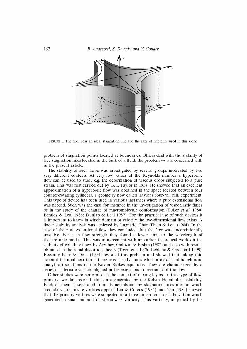
In the limit Ω = 0, the flow is irrotational with hyperbolic streamlines (figure 1).Whereas many works have been devoted to the study of rotating flows (where locallyγ Ω) and shear layers (where locally γ ' Ω), stretching flows (Ω ' 0) have receivedrelatively less attention from experimentalists, essentially because they are difficult togenerate and control.

The different investigations of the stability of three-dimensional stagnation pointflows can be classified into two distinct categories. Most works (see for instanceCriminale, Jackon & Lasseigne 1994 and references therein) are devoted to the

152 B. Andreotti, S. Douady and Y. Couder

z

y

x

Figure 1. The flow near an ideal stagnation line and the axes of reference used in this work.

problem of stagnation points located at boundaries. Others deal with the stability offree stagnation lines located in the bulk of a fluid, the problem we are concerned within the present article.

The stability of such flows was investigated by several groups motivated by twovery different contexts. At very low values of the Reynolds number a hyperbolicflow can be used to study e.g. the deformation of viscous drops subjected to a purestrain. This was first carried out by G. I. Taylor in 1934. He showed that an excellentapproximation of a hyperbolic flow was obtained in the space located between fourcounter-rotating cylinders, a geometry now called Taylor’s four-roll mill experiment.This type of device has been used in various instances where a pure extensional flowwas needed. Such was the case for instance in the investigation of viscoelastic fluidsor in the study of the change of macromolecule conformation (Fuller et al. 1980;Bentley & Leal 1986; Dunlap & Leal 1987). For the practical use of such devices itis important to know in which domain of velocity the two-dimensional flow exists. Alinear stability analysis was achieved by Lagnado, Phan Thien & Leal (1984). In thecase of the pure extensional flow they concluded that the flow was unconditionallyunstable. For each flow strength they found a lower limit to the wavelength ofthe unstable modes. This was in agreement with an earlier theoretical work on thestability of colliding flows by Aryshev, Golovin & Ershin (1982) and also with resultsobtained in the rapid distortion theory (Townsend 1976; Leblanc & Godeferd 1999).Recently Kerr & Dold (1994) revisited this problem and showed that taking intoaccount the nonlinear terms there exist steady states which are exact (although non-analytical) solutions of the Navier–Stokes equations. They are characterized by aseries of alternate vortices aligned in the extensional direction x of the flow.

Other studies were performed in the context of mixing layers. In this type of flow,primary two-dimensional eddies are generated by the Kelvin–Helmholtz instability.Each of them is separated from its neighbours by stagnation lines around whichsecondary streamwise vortices appear. Lin & Corcos (1984) and Neu (1984) showedthat the primary vortices were subjected to a three-dimensional destabilization whichgenerated a small amount of streamwise vorticity. This vorticity, amplified by the

An experiment on two aspects of the interaction between strain and vorticity 153

stretching in the stagnation regions, rolls up into periodic streamwise alternate vortices.This situation has been simulated experimentally by the flow between two rollers, andhas been captured on video by P. Carlotti, S. Obled & H. K. Moffatt (1998, personalcommunication).

Our interest in hyperbolic flows is due to yet another reason. It is related tothe interaction between stretching and rotation in fully developed turbulence andin particular to the relation between pressure fluctuations and coherent structures.Though they may appear remote from the problem at hand it is worth summarizingbriefly some results in this field.

The local structure of a turbulent flow can be characterized by the spatial distri-bution of strain tensor σij = (∂ivj + ∂jvi)/2 and vorticity ω = ∇× v. The evolution intime of the vorticity ωi is governed by the equation

∂tωi + vj∂jωi = σijωj + ν∂j∂jωi (1.2)

where ν is the kinematic viscosity. The term σijωi means that vorticity is amplified bya longitudinal stretching, corresponding to the conservation of angular momentum.This phenomenon, which is thought to dominate the dynamics of 3D turbulence, isnot yet well described in terms of elementary processes. The situation is complicatedbecause the strain tensor obeys an even more complex equation of evolution (Ohkitani& Kishiba 1995). It is not only advected and damped by viscosity but also evolvesunder the complicated effects of vorticity, strain and pressure. The equation governingits evolution is

∂tσij + vj∂jσij = 14(ωkωkδij − ωiωj)− σikσkj − ∂ijp+ ν∂j∂jσij . (1.3)

It is crucial to note that (1.3) is a non-local equation since pressure depends on thewhole flow (in particular on boundary conditions) through the Poisson law

∆p = 12ωiωi − σijσij . (1.4)

In reverse, relation (1.4) means that pressure measurements can be used to inves-tigate the spatial distribution of vorticity and strain. The existence of low-pressurefilaments in turbulent flows was demonstrated experimentally by Douady, Coudet &Brachet (1991). They correspond to rotating regions in which the vorticity is concen-trated in a thin core while the strain is spread at the periphery, as in a Burgers vortex(Burgers 1940). Correspondingly the fluctuations of pressure at one point were inves-tigated by Fauve, Laroche & Castaing (1993) and Cadot, Doudy & Couder (1995).Generally in these experiments as well as in previous numerical simulations (Brachet1991; Metais & Lesieur 1992) the probability distribution function of pressure ex-hibits a strong asymmetry with a long exponential tail towards the low pressures anda shorter Gaussian tail towards the high pressures. The low-pressure troughs are thesignature of filaments passing the probe. The absence of corresponding high-pressurepeaks is a clue pointing to the absence of organized high strain regions.

Numerical simulations permit direct observation of the structures present in turbu-lent flows. Since the initial work by Siggia (1981) a specific effort has been devotedto the detection of vortices in simulations of increasing spatial resolution (Jimenezet al. 1993; Jeong & Hussain 1995; Kida & Miura 1998). More generally the spatialdistribution of enstrophy ω2 = ωiωi and strain modulus σ2 = 2σijσij were investigatedby Tanaka & Kida (1993); Jimenez et al. (1993); Tsinober et al. (1997); Tsinober(1998); Nomura & Post (1999). The joined probability density functions show thatthere exist regions in which the vorticity is large and the strain small. When theseregions are singled out, they appear in the form of filaments. Similarly the regions


where both ω2 and σ2 are large are observed to be in the shape of sheets. Finally, theregions of large σ2 and small ω2 are far less probable and have no specific spatialstructure.

The first question that motivated the present work is thus: why are there noorganized regions of high strain and weak vorticity, i.e. no high-pressure structures?The observations in the mixing layers suggest that this is linked with the instabilityof hyperbolic regions. In between the main eddies there are stagnation lines whichshould be high-pressure regions. Instead it is well known that this is the locus offormation of secondary streamwise vortices. As observed by Douady et al. (1991),these streamwise vortices are low-pressure filaments. The paradox is that where highpressure is expected, low-pressure filaments form.

The second question is related to the enhancement of vorticity by stretching. Doesit occur mainly in strain-dominated regions or in organized vortices? In a preliminarywork (Andreotti, Doudy & Couder 1997) we showed, using two distinct experiments,that the vorticity stretching occurs mostly before the vortices are formed but thatthe stretching decreases after their formation. This effect was ascribed by Andreottiet al. (1997) to the two-dimensionalization of the flow near the core of rapidlyrotating vortices, an effect which results in a reduction of the longitudinal velocitygradient (Andreotti 1999). This observation is likely to be correlated with the resultsobtained on the statistics of enstrophy production in turbulent flows. From variousconditional averaging Tsinober, Ortenberg & Shtillman (1999) have demonstratedthat the enstrophy production is much larger in the regions dominated by strain thanin those dominated by enstrophy.

For all these reasons we wanted to do a direct experimental investigation of thestability of a pure strain flow in a model experiment and to observe the dynamicsof both stretching and vorticity in such regions. First aiming to obtain a well-controlled hyperbolic flow we were brought back to Taylor’s (1938) four-roll millexperiment. There is, to our knowledge, only one previous experimental investigationof the stability in this geometrical configuration, by Lagnado & Leal (1990). Theyfound, over a certain threshold, the formation of vortices aligned in the stretchingdirection. But in their experiment this array was limited to two vortices locatednear the extremities of the cylinders with one single recirculation vortex in between.This led them to conclude: ‘the vortices are primarily an end effect and a columnof alternate vortices does not appear throughout the entire vertical extent at largeraspect ratio. . . ’. Our experiments, done in a different geometry, lead to a differentconclusion.

The first part of this article deals with the instability of a hyperbolic flow at lowReynolds numbers. After a description of the experimental apparatus, we will discussthe two-dimensional stagnation point flow obtained at very low Reynolds numbersand describe its destabilization and the formation of a row of counter-rotating vorticesaligned in the stretching direction.

In the second part, we investigate the interaction between stretching and rotationin the same experiment but at high Reynolds numbers. We will present evidencethat there is a negative feedback of the rotation of the vortices on the stretching towhich they are submitted. As a conclusion, the consequences of such a mechanismfor turbulent flows will be discussed.

2. Experimental set-upThe design of a cell in which the flow has a pure strain field appears, at first sight,

to be impossible. Indeed, integrating the Poisson equation (1.4), we obtain the equality


y

y

x

x

d

D

(b)(a)

Figure 2. (a) Sketch of the experimental Taylor’s four-roller mill. Two details can be seen. Thecylinders are terminated by circular end plates which reduce the recirculation in this region. Fourwedges are glued onto the outer boundary and reduce the minimum distance between the rollersand the cell wall to d. They avoid the formation of Taylor–Couette rollers between the cylindersand the outer walls. (b) Transverse section of the experimental set-up.

of enstrophy and strain, on the average:

〈ω2〉 = 〈σ2〉. (2.1)

In fact, as was pointed out by Raynal (1996) this relation does not necessarily hold ina closed cell having moving boundaries. This is precisely the case in the four-rollersgeometry.

The core of the experiment is composed of four cylinders having parallel axes andplaced at the corners of a square (figure 2). The two cylinders placed on one diagonalrotate at one velocity, the two others at a second velocity. As is well known, all thelinear flows of the form (1.1) can be obtained in the central region of this apparatuswhen the fluid is very viscous and the rotation speed small. When the velocities ofthe cylinders are opposite, the flow is very close to the ideal hyperbolic flow:

vx = γx, vy = −γy. (2.2)

In the outer region of the cell, bounded by the container’s wall, most of the flowcorresponds to four halves of hyperbolic flows. Thus, globally in the whole cell theflow at low velocities is dominated by pure strain. The reason why it does notcontradict equation (2.1) is that the motion of the cylinders has to be taken intoaccount in the balance between strain and enstrophy. In these cells the vorticity couldbe said to be frozen inside the rotating cylinders while the strain is in the flow.

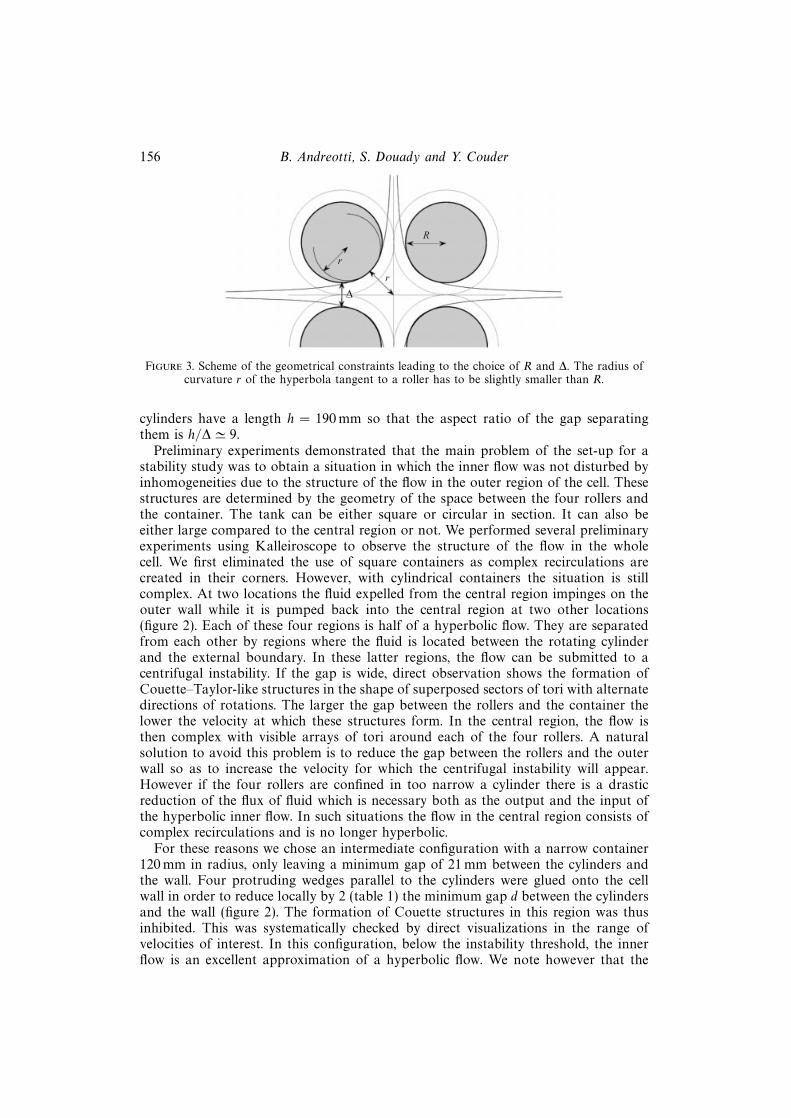
In practice, the radius R of the rollers and the gap ∆ between them can be chosenat will in order to obtain the best approximation of a hyperbolic flow. The distance(R + r) of the rollers axis to the centre of the cell (figure 3) is given by

(R + r)2 = 2(R + ∆/2)2. (2.3)

The hyperbola tangent to the rollers (figure 3) has a radius of curvature r. If Rwas chosen equal to r the hyperbola and the circle would have the same radiusof curvature at the point of tangency. Instead, we chose empirically a value of r(r = 29 mm) slightly smaller than R (R = 35 mm). For these values the two curves(the circle and the hyperbola) remain close to each other in a larger region (figure 3).The minimum distance between two adjacent cylinders is thus ∆ = 21 mm. The four


r

R

r

D

Figure 3. Scheme of the geometrical constraints leading to the choice of R and ∆. The radius ofcurvature r of the hyperbola tangent to a roller has to be slightly smaller than R.

cylinders have a length h = 190 mm so that the aspect ratio of the gap separatingthem is h/∆ ' 9.

Preliminary experiments demonstrated that the main problem of the set-up for astability study was to obtain a situation in which the inner flow was not disturbed byinhomogeneities due to the structure of the flow in the outer region of the cell. Thesestructures are determined by the geometry of the space between the four rollers andthe container. The tank can be either square or circular in section. It can also beeither large compared to the central region or not. We performed several preliminaryexperiments using Kalleiroscope to observe the structure of the flow in the wholecell. We first eliminated the use of square containers as complex recirculations arecreated in their corners. However, with cylindrical containers the situation is stillcomplex. At two locations the fluid expelled from the central region impinges on theouter wall while it is pumped back into the central region at two other locations(figure 2). Each of these four regions is half of a hyperbolic flow. They are separatedfrom each other by regions where the fluid is located between the rotating cylinderand the external boundary. In these latter regions, the flow can be submitted to acentrifugal instability. If the gap is wide, direct observation shows the formation ofCouette–Taylor-like structures in the shape of superposed sectors of tori with alternatedirections of rotations. The larger the gap between the rollers and the container thelower the velocity at which these structures form. In the central region, the flow isthen complex with visible arrays of tori around each of the four rollers. A naturalsolution to avoid this problem is to reduce the gap between the rollers and the outerwall so as to increase the velocity for which the centrifugal instability will appear.However if the four rollers are confined in too narrow a cylinder there is a drasticreduction of the flux of fluid which is necessary both as the output and the input ofthe hyperbolic inner flow. In such situations the flow in the central region consists ofcomplex recirculations and is no longer hyperbolic.

For these reasons we chose an intermediate configuration with a narrow container120 mm in radius, only leaving a minimum gap of 21 mm between the cylinders andthe wall. Four protruding wedges parallel to the cylinders were glued onto the cellwall in order to reduce locally by 2 (table 1) the minimum gap d between the cylindersand the wall (figure 2). The formation of Couette structures in this region was thusinhibited. This was systematically checked by direct visualizations in the range ofvelocities of interest. In this configuration, below the instability threshold, the innerflow is an excellent approximation of a hyperbolic flow. We note however that the


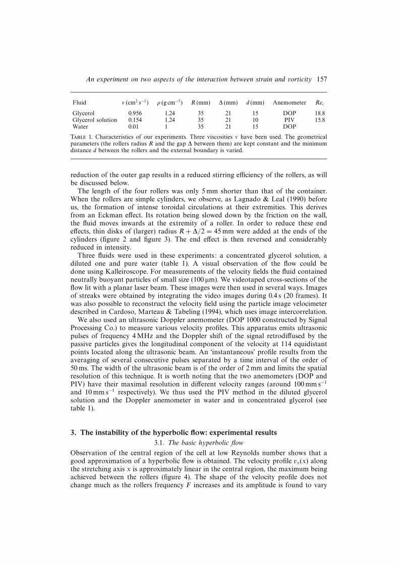
Fluid ν (cm2 s−1) ρ (g cm−3) R (mm) ∆ (mm) d (mm) Anemometer Rec

Glycerol 0.956 1.24 35 21 15 DOP 18.8Glycerol solution 0.154 1.24 35 21 10 PIV 15.8Water 0.01 1 35 21 15 DOP

Table 1. Characteristics of our experiments. Three viscosities ν have been used. The geometricalparameters (the rollers radius R and the gap ∆ between them) are kept constant and the minimumdistance d between the rollers and the external boundary is varied.

reduction of the outer gap results in a reduced stirring efficiency of the rollers, as willbe discussed below.

The length of the four rollers was only 5 mm shorter than that of the container.When the rollers are simple cylinders, we observe, as Lagnado & Leal (1990) beforeus, the formation of intense toroidal circulations at their extremities. This derivesfrom an Eckman effect. Its rotation being slowed down by the friction on the wall,the fluid moves inwards at the extremity of a roller. In order to reduce these endeffects, thin disks of (larger) radius R + ∆/2 = 45 mm were added at the ends of thecylinders (figure 2 and figure 3). The end effect is then reversed and considerablyreduced in intensity.

Three fluids were used in these experiments: a concentrated glycerol solution, adiluted one and pure water (table 1). A visual observation of the flow could bedone using Kalleiroscope. For measurements of the velocity fields the fluid containedneutrally buoyant particles of small size (100 µm). We videotaped cross-sections of theflow lit with a planar laser beam. These images were then used in several ways. Imagesof streaks were obtained by integrating the video images during 0.4 s (20 frames). Itwas also possible to reconstruct the velocity field using the particle image velocimeterdescribed in Cardoso, Marteau & Tabeling (1994), which uses image intercorrelation.

We also used an ultrasonic Doppler anemometer (DOP 1000 constructed by SignalProcessing Co.) to measure various velocity profiles. This apparatus emits ultrasonicpulses of frequency 4 MHz and the Doppler shift of the signal retrodiffused by thepassive particles gives the longitudinal component of the velocity at 114 equidistantpoints located along the ultrasonic beam. An ‘instantaneous’ profile results from theaveraging of several consecutive pulses separated by a time interval of the order of50 ms. The width of the ultrasonic beam is of the order of 2 mm and limits the spatialresolution of this technique. It is worth noting that the two anemometers (DOP andPIV) have their maximal resolution in different velocity ranges (around 100 mm s−1

and 10 mm s−1 respectively). We thus used the PIV method in the diluted glycerolsolution and the Doppler anemometer in water and in concentrated glycerol (seetable 1).

3. The instability of the hyperbolic flow: experimental results3.1. The basic hyperbolic flow

Observation of the central region of the cell at low Reynolds number shows that agood approximation of a hyperbolic flow is obtained. The velocity profile vx(x) alongthe stretching axis x is approximately linear in the central region, the maximum beingachieved between the rollers (figure 4). The shape of the velocity profile does notchange much as the rollers frequency F increases and its amplitude is found to vary


1.5

1.0

0.5

0

–0.5

–1.0

–1.5–3 –2 –1 0 1 2 3

x/R

vx

çR

Figure 4. Rescaled velocity profile along the extensional axis x for various frequenciesbetween F = 0.5 s−1 and F = 3 s−1, for the glycerol.

1

0

ç (s–1)

2

3

4

5

6

F (s–1)

0.5 1.0 1.5 2.0 2.5 3.0

Figure 5. The stretching coefficient γ as a function of the roller frequency F ,the working fluid being the glycerol.

proportionally to the cylinder frequency F . In particular the velocity gradient in thecentral region scales as F:

∂vx

∂x= γ = kF. (3.1)

The coefficients of proportionality in our experiments were k = 1.4 for the dilutedglycerol solution and k = 2.7 for the concentrated one (figure 5). These values areapproximately respectively a quarter and a half of that (k = 5.1) found by Taylor(1934). This difference is due to the fact that the efficiency of the rollers in settingthe fluid into motion is a function of the geometry of the whole cell. In Taylor’sexperiment the four rollers are surrounded by a large tank. In ours the flow is forcedthrough narrow gaps d (see table 1) between the rollers and the walls of the container,a hindrance to the stirring efficiency.

We will need a parameter to describe both the hyperbolic flow and its confinement.Because of the variation of the stirring efficiency we cannot use directly the frequencyof the cylinders to describe the physical situation. In a different tank (e.g. for a


(a) (b) (c)

Figure 6. Images of cross-sections of the flow in the plane (yOz) perpendicular to the stretching, forthe diluted glycerol solution. For each frequency, the whole field is shown on the left (visualizationusing Kalleiroscope) and a close-up view is shown on the right (visualization with spherical particles,integrating the video images for 0.4 s). (a) The hyperbolic flow at F = 0.3 Hz (or Re = 8.7) wellbelow the instability. (b) The flow at F = 0.55 Hz (or Re = 15.9) immediately above the threshold.(c) The flow at F = 0.66 Hz (or Re = 19.1) with a periodic array of alternate vortices.

different parameter d) the same velocities of the cylinders produce a different flow.The best parameter to describe the actual hyperbolic flow is thus the measured fluidvelocity gradient γ as given by equation (3.1). In particular, all the velocity profilesalong the extensional axis x collapse once rescaled using γ (figure 4). The flow being,in the central region, geometrically bounded by the rollers themselves we will chooseas the typical length scale the gap ∆ between them. From these two quantities weform a Reynolds number:

Re =γ∆2

ν. (3.2)

With this definition we find that below a critical value Rec the flow is stable (figure 6a).

3.2. Instability threshold

At the critical Reynolds number Rec ' 17, the central vertical line which separatesthe two colliding jets destabilizes into a sinusoid (figure 6b). For a slightly largervalue the formation of an array of steady alternate vortices is observed (figure 6c). Itis important to note that in this velocity range no other structure is observed in thecell. More specifically no tori due to a centrifugal instability exist near the cylinders.The observed instability affects the core of the hyperbolic flow. For this reason weare confident that the instability observed here is an intrinsic characteristic of thehyperbolic region, even though the visual evidence may appear insufficient to rule outcompletely any centrifugal effect. The distance separating two successive vortices in thevertical direction is of the order of the gap ∆ between the cylinders. At approximatelyRe ' 45 the vortices become chaotic. Well-defined vortices are observed in the wholerange of Reynolds numbers explored (up to 3000). It is worth noting that an internalReynolds number of 3000 (in water) corresponds to a Reynolds number based onthe rollers velocity and radius of 105.


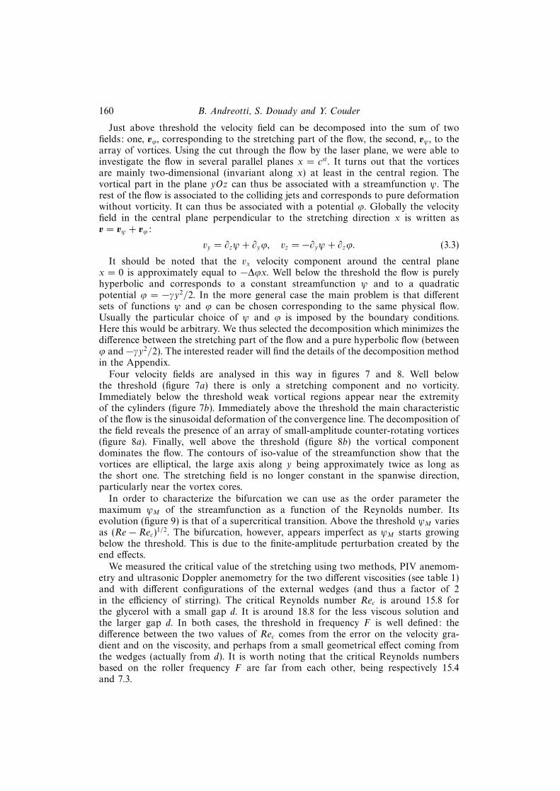
Just above threshold the velocity field can be decomposed into the sum of twofields: one, vϕ, corresponding to the stretching part of the flow, the second, vψ , to thearray of vortices. Using the cut through the flow by the laser plane, we were able toinvestigate the flow in several parallel planes x = cst. It turns out that the vorticesare mainly two-dimensional (invariant along x) at least in the central region. Thevortical part in the plane yOz can thus be associated with a streamfunction ψ. Therest of the flow is associated to the colliding jets and corresponds to pure deformationwithout vorticity. It can thus be associated with a potential ϕ. Globally the velocityfield in the central plane perpendicular to the stretching direction x is written asv = vψ + vϕ:

vy = ∂zψ + ∂yϕ, vz = −∂yψ + ∂zϕ. (3.3)

It should be noted that the vx velocity component around the central planex = 0 is approximately equal to −∆ϕx. Well below the threshold the flow is purelyhyperbolic and corresponds to a constant streamfunction ψ and to a quadraticpotential ϕ = −γy2/2. In the more general case the main problem is that differentsets of functions ψ and ϕ can be chosen corresponding to the same physical flow.Usually the particular choice of ψ and ϕ is imposed by the boundary conditions.Here this would be arbitrary. We thus selected the decomposition which minimizes thedifference between the stretching part of the flow and a pure hyperbolic flow (betweenϕ and −γy2/2). The interested reader will find the details of the decomposition methodin the Appendix.

Four velocity fields are analysed in this way in figures 7 and 8. Well belowthe threshold (figure 7a) there is only a stretching component and no vorticity.Immediately below the threshold weak vortical regions appear near the extremityof the cylinders (figure 7b). Immediately above the threshold the main characteristicof the flow is the sinusoidal deformation of the convergence line. The decomposition ofthe field reveals the presence of an array of small-amplitude counter-rotating vortices(figure 8a). Finally, well above the threshold (figure 8b) the vortical componentdominates the flow. The contours of iso-value of the streamfunction show that thevortices are elliptical, the large axis along y being approximately twice as long asthe short one. The stretching field is no longer constant in the spanwise direction,particularly near the vortex cores.

In order to characterize the bifurcation we can use as the order parameter themaximum ψM of the streamfunction as a function of the Reynolds number. Itsevolution (figure 9) is that of a supercritical transition. Above the threshold ψM variesas (Re − Rec)1/2. The bifurcation, however, appears imperfect as ψM starts growingbelow the threshold. This is due to the finite-amplitude perturbation created by theend effects.

We measured the critical value of the stretching using two methods, PIV anemom-etry and ultrasonic Doppler anemometry for the two different viscosities (see table 1)and with different configurations of the external wedges (and thus a factor of 2in the efficiency of stirring). The critical Reynolds number Rec is around 15.8 forthe glycerol with a small gap d. It is around 18.8 for the less viscous solution andthe larger gap d. In both cases, the threshold in frequency F is well defined: thedifference between the two values of Rec comes from the error on the velocity gra-dient and on the viscosity, and perhaps from a small geometrical effect coming fromthe wedges (actually from d). It is worth noting that the critical Reynolds numbersbased on the roller frequency F are far from each other, being respectively 15.4and 7.3.


1 cm s–1(a)

z

y

1 cm s–1(b)

v vã vu

Figure 7. The velocity field in the plane x = 0 for two rotation frequencies below the instabilitythreshold: (a) F = 0.25 Hz (Re = 7.2); (b) F = 0.50 Hz (Re = 14.5). In each case the actual velocityfield v is given on the left. It is decomposed into a two-dimensional vortical component vψ (centre)and in an irrotational stretching part (right) vϕ.

4. The instability of the hyperbolic flow: theoretical aspects4.1. Linear stability analysis

The linear stability analysis of the idealized hyperbolic flow (2.2) shows that it isalways unstable. Several variants of this analysis can be found in Aryshev et al.(1982); Lagnado et al. (1984); Craik & Criminale (1986) (who use the growth ofFourier modes), Leblanc & Godeferd (1999) (who use the rapid distortions theory),Lin & Corcos (1984), Neu (1984) and Criminale et al. (1994). Basically the instabilityis due to the amplification by stretching of vortical disturbances. This is particularlyeasy to see at the stagnation point where the velocity is null so that the equationgoverning the vorticity reduces to

∂tωx = γωx, ∂tωy = −γωy, ∂tωz = 0. (4.1)


1 cm s–1(a)

z

y

1 cm s–1(b)

v vã vu

1 cm s–1 1 cm s–1

1 cm s–1 1 cm s–1

ã

Figure 8. As figure 8 but for two rotation frequencies located above the threshold: (a) F = 0.55 Hz(Re = 15.9); (b) F = 0.65 Hz (Re = 19.1). The streamlines (iso ψ) are shown on the right.

Of particular interest for comparison with the experimental results is the workof Kerr & Dold (1994) who obtained by semi-analytical means a family of exactstationary solutions. They correspond to a periodic array of counter-rotating vorticesaligned in the stretching direction x. The class of solution has two free parameters:the amplitude ω0 and the wavenumber k of the fundamental mode. This calculationdemonstrates that the nonlinearities do not change the flow fundamentally: thesolutions of the linearized problem are very close to being exact solutions of the fullNavier–Stokes equation. It should be understood that neither the amplitude nor thewavelength are selected by nonlinearities: they only induce the growth of harmonics.

For this reason we will limit ourselves here to the solutions of the linearizedequations, emphasizing the parameters relevant for comparison with the experimentalresults. We also propose an explicit solution of the equation, which had not been givenby the previous authors. The interested reader should consult Kerr & Dold’s (1994)


1

0

ãM (cm2 s–1)2

3

4

F (s–1)

0.45 0.50 0.55 0.60 0.65 0.700.40

Figure 9. The instability threshold. The evolution of an order parameter (the maximum ψM of thestreamfunction) as a function of the control parameter, the rotation frequency of the rollers.

article for the nonlinear analysis of the problem and the asymptotic development ofthe solutions.

4.2. Explicit solution of the linearized problem

The unstable modes are invariants along x and can be written using a streamfunc-tion ψ:

vx = γx, vy = −γy + ∂zψ, vz = −∂yψ. (4.2)

Neglecting the advection generated by the disturbances themselves the equation forthe x-component of the vorticity is

∂tωx = γ∂x(xωx) + ν∆ωx. (4.3)

Since there is no advection of the vorticity along the z-axis the disturbance can bedeveloped in Fourier modes along this direction:

ωx = ω0f(y`

)cos(kz) (4.4)

with f(0) = 1 and f′′(0) = −1.As in the experiment the disturbance is thus a periodic array of counter-rotating

vortices aligned along x, the stretching direction; ω0 is the vorticity at the core ofthe vortices, k the wavenumber in the z-direction and ` the vortex typical size in thedirection of the compression y. The vorticity is the opposite of the streamfunction’sLaplacian. We can write:

ψ = `2ω0g(y`

)cos(kz) (4.5)

with g′′ − (k`)2g = −f. While g is defined up to a hyperbolic cosine it becomes uniqueif it has to vanish at infinity: g(+∞) = 0. We first seek stationary solutions. Insertingωx of the form (4.4) in the vorticity equation (4.3) we get a differential equation for f:

f′′(ζ) +γ`2

νζf′(ζ) + `2

(γν− k2

)f(ζ) = 0. (4.6)

Using the condition defining `, f′′(0) = −1, we get a relation among the stretching γ,


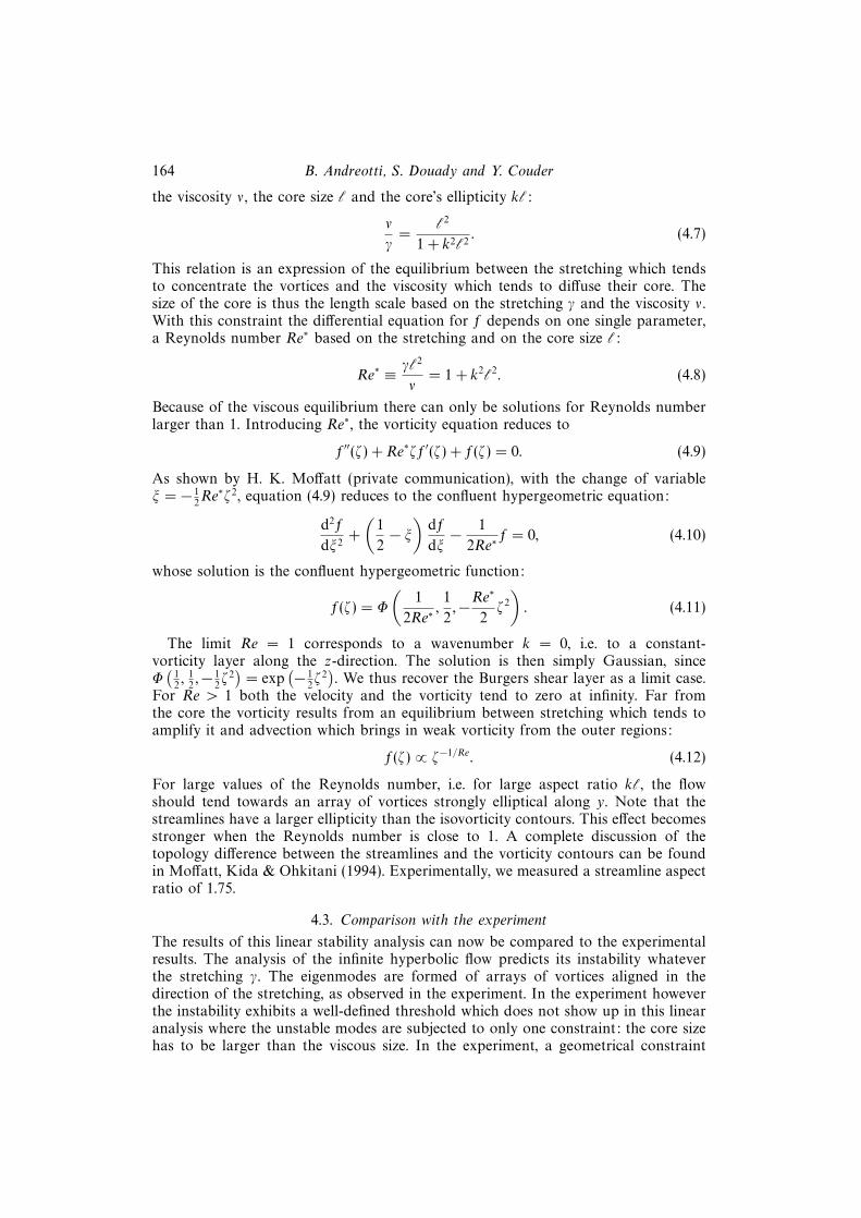
the viscosity ν, the core size ` and the core’s ellipticity k`:

ν

γ=

`2

1 + k2`2. (4.7)

This relation is an expression of the equilibrium between the stretching which tendsto concentrate the vortices and the viscosity which tends to diffuse their core. Thesize of the core is thus the length scale based on the stretching γ and the viscosity ν.With this constraint the differential equation for f depends on one single parameter,a Reynolds number Re∗ based on the stretching and on the core size `:

Re∗ ≡ γ`2

ν= 1 + k2`2. (4.8)

Because of the viscous equilibrium there can only be solutions for Reynolds numberlarger than 1. Introducing Re∗, the vorticity equation reduces to

f′′(ζ) + Re∗ζf′(ζ) + f(ζ) = 0. (4.9)

As shown by H. K. Moffatt (private communication), with the change of variableξ = − 1

2Re∗ζ2, equation (4.9) reduces to the confluent hypergeometric equation:

d2f

dξ2+

(1

2− ξ)

df

dξ− 1

2Re∗f = 0, (4.10)

whose solution is the confluent hypergeometric function:

f(ζ) = Φ

(1

2Re∗,1

2,−Re

∗

2ζ2

). (4.11)

The limit Re = 1 corresponds to a wavenumber k = 0, i.e. to a constant-vorticity layer along the z-direction. The solution is then simply Gaussian, sinceΦ(

12, 1

2,− 1

2ζ2)

= exp(− 1

2ζ2). We thus recover the Burgers shear layer as a limit case.

For Re > 1 both the velocity and the vorticity tend to zero at infinity. Far fromthe core the vorticity results from an equilibrium between stretching which tends toamplify it and advection which brings in weak vorticity from the outer regions:

f(ζ) ∝ ζ−1/Re. (4.12)

For large values of the Reynolds number, i.e. for large aspect ratio k`, the flowshould tend towards an array of vortices strongly elliptical along y. Note that thestreamlines have a larger ellipticity than the isovorticity contours. This effect becomesstronger when the Reynolds number is close to 1. A complete discussion of thetopology difference between the streamlines and the vorticity contours can be foundin Moffatt, Kida & Ohkitani (1994). Experimentally, we measured a streamline aspectratio of 1.75.

4.3. Comparison with the experiment

The results of this linear stability analysis can now be compared to the experimentalresults. The analysis of the infinite hyperbolic flow predicts its instability whateverthe stretching γ. The eigenmodes are formed of arrays of vortices aligned in thedirection of the stretching, as observed in the experiment. In the experiment howeverthe instability exhibits a well-defined threshold which does not show up in this linearanalysis where the unstable modes are subjected to only one constraint: the core sizehas to be larger than the viscous size. In the experiment, a geometrical constraint


2

0

zM (cm)4

6

8

F (s–1)

0.45 0.50 0.55 0.60 0.650.40

10

Dpk

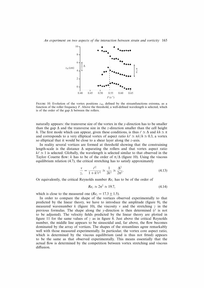
Figure 10. Evolution of the vortex positions zM , defined by the streamfunctions extrema, as afunction of the roller frequency F . Above the threshold, a well-defined wavelength is selected, whichis of the order of the gap ∆ between the rollers.

naturally appears: the transverse size of the vortex in the y-direction has to be smallerthan the gap ∆ and the transverse size in the z-direction smaller than the cell heighth. The first mode which can appear, given these conditions, is thus ` ' ∆ and kh ' πand corresponds to a very elliptical vortex of aspect ratio k` ' πδ/h ' 0.3, a vortexso elliptical that it would be close to a shear layer along the z-axis.

In reality several vortices are formed at threshold showing that the constraininglength-scale is the distance ∆ separating the rollers and that vortex aspect ratiok` ' 1 is selected. Globally, the wavelength is selected similar to that observed in theTaylor–Couette flow: k has to be of the order of π/∆ (figure 10). Using the viscousequilibrium relation (4.7), the critical stretching has to satisfy approximately

ν

γc=

`2

1 + k2`2' 1

2k2' ∆2

2π2. (4.13)

Or equivalently, the critical Reynolds number Rec has to be of the order of

Rec ' 2π2 ' 19.7, (4.14)

which is close to the measured one (Rec = 17.3± 1.5).In order to compare the shape of the vortices observed experimentally to that

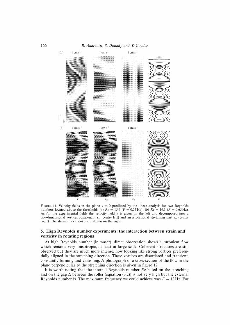
predicted by the linear theory, we have to introduce the amplitude (figure 9), themeasured wavenumber k (figure 10), the viscosity ν and the stretching γ in theprevious formulas. The shape along the y-direction is then determined (` is notto be adjusted). The velocity fields predicted by the linear theory are plotted infigure 11 for the same values of γ as in figure 8. Just above the critical Reynoldsnumber, the middle line appears to be sinusoidal and, far above, the flow becomesdominated by the array of vortices. The shapes of the streamlines agree remarkablywell with those measured experimentally. In particular, the vortex core aspect ratio,which is determined by the viscous equilibrium (and is thus not fitted) appearsto be the same as that observed experimentally. This means essentially that theactual flow is determined by the competition between vortex stretching and viscousdiffusion.


1 cm s–1(a)

z

y

1 cm s–1(b)

v vã vu

1 cm s–1 1 cm s–1

1 cm s–1 1 cm s–1

ã

Figure 11. Velocity fields in the plane x = 0 predicted by the linear analysis for two Reynoldsnumbers located above the threshold: (a) Re = 15.9 (F = 0.55 Hz); (b) Re = 19.1 (F = 0.65 Hz).As for the experimental fields the velocity field v is given on the left and decomposed into atwo-dimensional vortical component vψ (centre left) and an irrotational stretching part vϕ (centreright). The streamlines (iso-ψ) are shown on the right.

5. High Reynolds number experiments: the interaction between strain andvorticity in rotating regions

At high Reynolds number (in water), direct observation shows a turbulent flowwhich remains very anisotropic, at least at large scale. Coherent structures are stillobserved but they are much more intense, now looking like strong vortices preferen-tially aligned in the stretching direction. These vortices are disordered and transient,constantly forming and vanishing. A photograph of a cross-section of the flow in theplane perpendicular to the stretching direction is given in figure 12.

It is worth noting that the internal Reynolds number Re based on the stretchingand on the gap ∆ between the roller (equation (3.2)) is not very high but the externalReynolds number is. The maximum frequency we could achieve was F = 12 Hz. For


Figure 12. Close-up view of a cross-section of the flow in the median plane yOz of the cell(perpendicular to the stretching direction x) in the turbulent regime at Re ' 1600. Two vortices anda stagnation point can be seen.

this value, the internal Reynolds number is slightly larger 3000 while the Reynoldsnumber based on the roller velocities and on their radius is of the order of 105.

We performed a series of measurements of the velocity profile vx(x) across the wholecell, in the stretching direction x (the measurement which gave us the value of theparameter γ (figure 4)). Below the instability threshold it is steady and independentof the position on the z-axis. At high Reynolds number the profile vx(x) fluctuates.For most of the time it is noisy due only to the turbulence of the fluid but retains asimilar global profile. However, intermittently, the whole velocity gradient is stronglyreduced for a short time. Since particles are present in the flow for the ultrasonicanemometry, it is possible to simultaneously measure the velocity profile and visualizethe flow. This systematic comparison of the visual appearance of the flow with thecorresponding measurements requires two observers: one to watch the flow itself, thesecond to look at the fluctuating profile on the computer screen. We were able in thisway to observe that all the profiles having a weak gradient were those obtained at theprecise moment when the core of a vortex passed in front of the probe (with its axisalong the direction of measurement). In reverse we also checked that all the vorticespassing the probe generated a weakening of the gradient.

The average profile is well defined: it is shown (at F = 6 Hz) by the open circleson the four plots of figure 13. The velocity gradient induced by the rollers is clearlyvisible; it is practically constant from z = −45 mm to z = +45 mm, i.e. in the wholecentral region of the cell. Its value is γ = 3.6 s−1, i.e. 0.6F . Two instantaneous profilestaken at random times are shown for comparison on figure 13(a) (black circles). Inspite of local turbulent fluctuations they exhibit the same global velocity gradient.

Since we could visualize the flow during the measurements, we also triggered instan-taneous measurements of vx(x) at the exact moment when the axis of one of the turbu-lent vortices coincided with the axis of the ultrasonic probe. Two examples of such pro-files are shown on figure 13(b) (black circles). The velocity gradient along the axis of avortex is clearly weaker than the average gradient and of the order of γ = 0.7 s−1 only.

6. Discussion: the dynamics of interaction between strain and vorticityWe can now return to turbulence. Our present results can contribute to a phe-

nomenological interpretation of recently observed characteristics of turbulent flows.


20

10

–6 –4 42

–20

x (cm)v x

(cm

s–1

)(a)20

10

–4 42

–20

x (cm)

v x (

cm s

–1)(b)

–10

–20

–10–6 –4 42

x (cm)

20

10v x (

cm s

–1)(c)

–4 42

–20

x (cm)–10–6

20

10v x (

cm s

–1)(d)

Figure 13. Longitudinal velocity profiles in the stretching direction at a rotation frequency ofF = 6 Hz corresponding to a Reynolds number Re ' 1600. The origin of the abscissa is chosenin the centre of the cell and the narrowest gap between the cylinders is at z = 4.5 cm. The opencircles show the mean velocity profile, obtained by averaging 1024 instantaneous profiles. (a) Theblack circles are two instantaneous profiles chosen at random times. (b) The black circles are twoinstantaneous profiles chosen at the precise time where the axis of a vortex coincided with the axisof the ultrasonic beam.

They are particularly related to the recently investigated pressure fluctuations and tothe existence and dynamics of coherent structures. Statistically, a well-documentedresult is that the pressure fluctuations in a fully developed turbulent flow have anasymmetric distribution (Brachet 1991; Metais & Lesieur 1992; Fauve et al. 1993;Cadot et al. 1995). On the low-pressure side the probability distribution functionhas a long exponential tail due to rare events with large depressions. In contrastthe high-pressure side has a shorter Gaussian tail. Because of the Poisson law (1.4)the pressure field reflects the spatial distribution of vorticity and strain. As shownexperimentally by Cadot et al. (1995) the large depressions which are observed (atone point) as intermittent bursts are associated with intense vorticity filaments whichhave been observed directly both numerically (Siggia 1981; Tanaka & Kida 1993;Jimenez et al. 1993) and experimentally (Douady et al. 1991; Cadot et al. 1995). Thesestructures form in a region with large stretching. Briefly they are coherent and ratherstraight, before finally disappearing in a kind of vortex breakdown.

6.1. Regions of large strain and weak vorticity

The intrinsic instability of the regions of pure strain had already been observed in thecontext of the formation of the secondary streamwise vortices of mixing layers (Lin& Corcos 1984; Neu 1984). Here we have investigated this instability in a controlledsystem and most of the characteristics that had been predicted theoretically havebeen observed. We thus have a situation in which vortices (low-pressure structures)are spontaneously formed in the regions of pure strain (high-pressure regions). Whilein such regions, the initial viscous flow contains almost no vorticity, it is unstable andtransforms into a flow dominated by vortices. Where does the vorticity come from?


This paradox is only an apparent one: the hyperbolic flows are opened and suck inperturbations from the outside. Vorticity is thus captured, stretched and amplified,and feeds the instability.

The existence of a finite threshold in our experiment is directly linked with thefinite extension of the experimental domain and with the corresponding limitation inwavenumber k. We believe that, in turbulence, whenever a region of nearly pure purestrain forms (by the interaction of neighbouring structures) it is intrinsically unstable.This instability process is likely to be responsible for the short lifetime and thus thescarcity of regions of pure strain and high pressure in turbulence.

This observation is in very good agreement with the results obtained on the statisticsof enstrophy production in turbulent flows. From various conditional averagingTsinober et al. (1999) have demonstrated that the enstrophy production is muchlarger in the regions dominated by strain than in those dominated by enstrophy.

6.2. Regions of large vorticity and weak strain

Our experiment, because of its geometry, seems to impose a well-determined longitu-dinal velocity gradient in the central region of the cell. This reproduces the conditionsimposed on the theoretical solutions by Kerr & Dold (1994). In these solutions, as inall Burgers-like models (Burgers 1940), the stretching is an imposed field. The excel-lent agreement obtained between the experimentally observed flow and the theoreticalone seems to validate this assumption in the low Reynolds number range.

At high Reynolds numbers however, as demonstrated in the previous section, thelongitudinal velocity gradient is observed to be reduced in the vortex core region. Ourhypothesis is that this effect is related to the two-dimensionalization due to the fastrotation near the core of axisymmetric vortices. In order to check this hypothesis wealso investigated vortex stretching in a different configuration (Andreotti et al. 1997).We performed a variant of a classical experiment (Escudier 1984) in which a vortex iscreated in a cylindrical tank having a rotating disk at one end. In this experiment weintroduced the possibility of pumping the fluid out of the cell through a hole locatedalong the cell axis (the fluid being reinjected beneath the disk). When this suction isactivated there is a transitory formation of a longitudinal velocity gradient along thevortex axis and intensification of this vortex. When the flow has become steady thevortex is very intense, and the velocity along its axis is large but the gradient of thisvelocity is drastically reduced (Andreotti et al. 1997).

In this latter experiment as well as in Taylor’s four-roll mill, the observed effect isthe same. The stretching of a vortex results in an intensification of its rotation. Inturn this rotation tends to make the flow two-dimensional in the core and thus tooppose the variations of velocity in this region. This effect, as it reduces the velocitygradients, diminishes the stretching. There is thus a negative feedback of the vorticeson the stretching which has generated them. This is a kind of Lenz law which hadnot been considered before.

The feedback mechanism is mainly that of Eckman pumping: when the stretchingis inhomogeneous, it induces variations of the vortex rotation along its axis. Thepressure gradient cannot balance the centrifugal force anymore, the latter havingsolenoidal part. As a consequence, the centrifugal force induces a radial flow in thepart of the vortex where the rotation is the fastest and thus reduces the stretchingin the vortex core. Globally, the vortex tends to reduce the stretching to which itis submitted, as soon as the stretching is localized in space. In another paper, wehave investigated numerically (Abid et al. 2001) this mechanism of interaction. Inparticular, we have shown that the typical timescale of the feedback of rotation on


stretching scales as L/Urotation where L is the characteristic length over which thestretching is inhomogeneous (it is also the length of the vortex) and Urotation is thetypical rotation velocity. The characteristic timescale of the vortex stretching is theinverse of the stretching γ. The ratio of the two,

B =Urotation

γL, (6.1)

gives a non-dimensional parameter which characterizes the relative importance of thefeedback mechanism and of the stretching process. For small B, the reaction can beneglected. In the limit case of homogeneous stretching, i.e. for Burgers-like vortices(Burgers 1940), L tends to infinity and B tends to zero: there is strictly no reaction. Assoon as the rotation becomes important when compared to the stretching (if B 1),the negative feedback of rotation on stretching must play a crucial role.

As a result, though the analytical solutions are good descriptions of the structuresobserved near the instability threshold, they fail to describe the situation at highReynolds number because they do not take into account the negative feedback ofrotation on stretching. In more recent models (Donaldson & Sullivan 1960; Gibbon,Fokas & Doering 1999; and Khomenko & Babiano 1999) the spatial homogeneity ofthe stretching has been relaxed, but it remains an imposed field. Our results show thatin experimental situations the stretching is of finite extension and that the negativefeedback of the vorticity on the stretching has drastic consequences. This effect shouldbe taken into account in more realistic models of vortices.

This new mechanism has implications for turbulent flows. In all regions wherevorticity is much larger than strain there is necessarily rotation, and this effect shouldappear. It is now well established by numerical simulations and experiments thatmost of the intense vorticity is concentrated in filament-like rotating structures. Thetwo-dimensionalization of these vortices linked to their rotation provides a physicalinterpretation of the straightness of the vortex filaments observed in turbulent flows.This was observed experimentally by Cadot et al. (1995), demonstrated on theoreticalgrounds by Constantin, Procaccia & Segel (1995) and observed numerically by Galanti,Procaccia & Segel (1996). The corresponding reduction of the strain along the axiscould also be responsible for the breakdown of the filaments which occurs ultimately.

It is often believed that the amplification of vorticity in turbulent flows is en-hanced by nonlinear effects. This was proved wrong by Ohkitani (1998) who recentlycompared the stretching of a passive vector and that of the vorticity. The equationsgoverning these two effects have similar linear terms and different nonlinear terms.The results of his numerical simulations demonstrate that, in a turbulent flow, thestretching of the vorticity is much weaker than that of passive vectors. The essentialdifference between the two is related to the relative orientations of the observedvector with the axes of strain. During its evolution the direction of the passive vectorhas no particular relation with the direction of the strain. In contrast, vorticity andstrain being both constructed from the velocity derivatives have directions which arestrongly related. Corresponding, as shown by Ohkitani (1998), the equation governingthe passive vector evolution is linear while that concerning vorticity is nonlinear. Inboth cases the linear term has the same stretching effect on the passive vector andon vorticity. The weaker stretching of vorticity means that the nonlinear effects dueto the alignments limit the stretching. We propose that the processes that we observeare the basis of the reduction of the vorticity stretching by nonlinearities. In theregions of high strain there is spontaneous collection and intensification of vorticityresulting in the formation of rotating regions. The rotation of these vortices generates


a negative feedback on stretching. These two effects could be the basic processesexplaining Okhitani’s result.

Finally, the negative feedback of rotation on stretching is a mechanism present inturbulence at all scales. At any scale, a coarse-grained vorticity and a coarse-grainedstrain tensor can be defined using for instance the velocity at the vertex of a tetrad(Chertkov, Pumir & Shraiman 1999). Like the actual vorticity and strain, the inertialeffects can be interpreted as vortex stretching and centrifugal force at the scale underconsideration. It was shown numerically by Chertkov et al. (1999) that at all scales,on the average, the pressure tends to counteract the effect of inertia but balances onlypart of it. This means that in rotating regions, the centrifugal force tends to expel thefluid from the centre of rotation and thus to reduce the stretching.

7. ConclusionThe instability of hyperbolic flows had already been investigated theoretically and

was known to occur in the secondary instabilities of mixing layers. Here we haveshown that a controlled version of this instability could be obtained in Taylor’s four-roll mill experiment. In this set-up the flow which is stable at low Reynolds numbers,destabilizes by a supercritical bifurcation at a well-defined threshold and forms anarray of counter-rotating vortices. The transverse velocity profiles of these vortices arein excellent agreement with those predicted by the theory of Kerr & Dold (1994). Theinstability threshold is well understood as resulting from the geometrical confinementof the flow.

We have also investigated this flow at high Reynolds number and the results thusobtained are relevant to the dynamics of the stretching of vorticity in turbulent flows.They can be summarized as follows:

(i) The regions of pure strain are highly unstable and are the locus of formation oforganized vortices. This result is in good agreement with the observation by Tsinoberet al. (1999) that these regions are statistically those of largest enstrophy production.

(ii) When strong vortices have formed the two-dimensionalization due to rotationreacts to reduce the stretching in their core. This nonlinear effect is in agreement withthe weak enstrophy production observed in these regions by Tsinober (1998), withthe alignments observed by Nomura & Post (1998) and with the results by Ohkitani(1998) on the nonlinear limitation of vortex stretching.

We are grateful to J. C. Sutra Fourcarde, H. Demaie and B. de Runz for their helpduring the experiment, and to J. Paret and O. Cardoso for the use of their PIV system.We wish to thank H. K. Moffatt who actually solved equation (4.9). A part of thisarticle was written during a stay of Y.C. at the Isaac Newton Institute in Cambridge,the other while B.A. was participating in the turbulent program of the Institute forTheoretical Physics in Santa Barbara. Both institutes are thanked for their hospitality.This research was supported in part by the National Science Foundation under GrantNo. PHY94-07194.

Appendix. Decomposition of the velocity field into a vortical and astretching part

We want to decompose the velocity field in the central plane into a rotational partand a potential part:

vy = ∂zψ + ∂yϕ, vz = −∂yψ + ∂zϕ. (A 1)


The main problem is that different sets of functions ψ and ϕ can be chosen corre-sponding to the same physical flow. If we consider a different potential ϕ′ which hasthe same Laplacian as ϕ (so that ∆(ϕ′ −ϕ) = 0), there exists a second streamfunctionψ′ which satisfies ∂z(ψ

′ − ψ) = −∂y(ϕ′ − ϕ) and ∂y(ψ′ − ψ) = ∂x(ϕ

′ − ϕ). As a con-sequence, (ϕ, ψ) and (ϕ′, ψ′) correspond to the same velocity field. In this particularexperiment, it would be arbitrary to use boundary conditions to determine ψ and ϕ.

Specifically, we wish to compare the velocity field measured experimentally to ahyperbolic flow disturbed by an array of vortices. This would mean a field of theform

vy = ∂zψ − γy, vz = −∂yψ. (A 2)

The best choice among the possible couples (ϕ, ψ) is that which minimizes thedifference between the stretching part of the flow and a pure hyperbolic flow. Supposethat we know the couple (ϕ0, ψ0) which satisfies (A 1) in a rectangular region Stogether with the boundary condition ϕ0 = 0. We want to find the potential ϕ andthe stretching γ which minimizes the surface integral:∫

S

[(∂yϕ+ γy)2 + (∂zϕ)2]ds (A 3)

under the constraint that everywhere in the rectangle ∆(ϕ − ϕ0) = 0. The solutionis easy to obtain: ϕ is the solution of ∆ϕ = ∆ϕ0 with the boundary conditionϕ = −γy2/2 and γ is given by the integral relation

γ =

∫S

−y∂yϕds∫S

y2ds

. (A 4)

In practice, an iterative procedure can be used to solve these coupled equations. Aregular grid is used and the velocity derivatives are estimated by finite differences. Wefirst find the field of the form (A 2) closest to the experimental measurements. To dothis, we minimize with respect to ψj,k and γ the usual likelihood functional L basedon the differences between the model velocity field and the experimental one:

L =1

2

∑j,k

(vj,k+1/2y − (ψj,k+1 − ψj,k) + γj)2 + (v

j+1/2,kz + (ψj+1,k − ψj,k))2

σ2j,k

. (A 5)

Note that each velocity measurement is weighted by the experimental standarddeviation σj,k measured for each mesh point. Note also that ψj,k is defined up to aconstant. We chose this constant in order that the maximum and minimum values ofψj,k be opposite. This leads to a system of linear equations coupling the values of ψat each grid point and γ which is solved numerically by a simple matrix inversion.

After this first step, we obtain an approximation of the measured velocity field inwhich the stretching field is spatially homogeneous. We then compute the differenceδv between the initial field and its projection:

δvy = vy − ∂zψ + γy, δvz = vz + ∂yψ. (A 6)

In most of the cases, this difference is already small compared to the velocity itself,meaning that expression (A 2) is a good approximation of the actual flow. We thenfind the potential field ∇ε closest to δv (in the least-square sense) and satisfying theboundary condition ε = ϕ+ γy2/2 = 0 derived above.


Again we compute the difference between the total velocity field v and ∇ε andseek ψj,k and γ minimizing the likelihood functional L. And again the best potentialε is determined. This process is iterated until convergence is achieved. In practiceonly three iterations of the type described above are necessary before obtaining asatisfactory decomposition (the rest being of the order of the noise). Adding the γand ε contributions, the potential is finally ϕ = −γy2/2 + ε.

REFERENCES

Abid, M., Andreotti, B., Douady, S. & Nore C. 2001 Oscillating structures in a stretched-compressed vortex. J. Fluid Mech. (submitted).

Andreotti, B. 1999 Action et reaction entre etirement et rotation, du laminaire au turbulent. PhDThesis report, Universite Paris 7, Paris.

Andreotti, B., Douady, S. & Couder, Y. 1997 About the interaction between vorticity andstretching in coherent structures. In Turbulence Modelling and Vortex Dynamics (ed. O. Boratav& A. Erzan), pp. 92–108. Springer.

Aryshev, Y. A., Golovin, V. A. & Ershin, S. A. 1982 Stability of colliding flows. Fluid Dyn. 1,755–759.

Bentley, B. J. & Leal, L. G. 1986 A computer controlled four-roll mill for investigations of particleand drop dynamics in two-dimensional linear shear flows. J. Fluid Mech. 167, 219–240.

Brachet, M. E. 1991 Direct simulation of three-dimensional turbulence in the Taylor-Green vortex.Fluid Dyn. Res. 8, 1–8.

Burgers, J. M. 1940 Application of a model system to illustrate some points of the statistical theoryof free turbulence. Proc. Acad. Sci. Amsterdam 43, 2–12.

Cadot, O., Douady, S. & Couder, Y. 1995 Characterisation of the low-pressure filaments in a threedimensional turbulent shear flow. Phys. Fluids 7, 630–646.

Cardoso, O., Marteau, D. & Tabeling, P. 1994 Quantitative experimental study of the free decayof quasi two-dimensional turbulence. Phys. Rev. E 49, 454–460.

Chertkov, B., Pumir, A. & Shraiman, B. 1999 Lagrangian tetrad dynamics and the phenomenologyof turbulence. Phys. Fluids 11, 2394–2412.

Constantin, P., Procaccia, I. & Segel, D. 1995 Creation and dynamics of vortex tubes in three-dimentionnal turbulence. Phys. Rev. E 51, 3207–3222.

Craik, A. D. D. & Criminale, W. O. 1986 Evolution of wavelike disturbances in shear flows: aclass of exact solution of Navier-Stokes equations. Proc. R. Soc. Lond. A 406, 13–26.

Criminale, W. O., Jackson, T. L. & Lasseigne, D. G. 1994 Evolution of disturbances in stagnation-point flow. J. Fluid Mech. 270, 331–347.

Donaldson, C. D. & Sullivan, R. D. 1960 Behaviour of solutions of the Navier-Stokes equationsfor a complete class of three-dimensional viscous vortices. In Proc. Heat Transfer & FluidMech. Inst., Stanford University.

Douady, S., Couder, Y. & Brachet, M. E. 1991 Direct observation of the intermittency of intensevorticity filaments in turbulence. Phys. Rev. Lett. 67, 983–986.

Dunlap, D. & Leal, L. G. 1987 Dilute polystyrene solutions in extensional flows – Birefringenceand flow modification. J. Non-Newtonian Fluid 23, 5–48.

Escudier, M. P. 1984 Vortex breakdown: observations and observations. Exps. Fluids 2, 189–196.

Fauve, S., Laroche, C. & Castaing, B. 1993 Pressure fluctuations in swirling turbulent flows.J. Phys. Paris II 3, 271–278.

Fuller, G. G, Rallison, J. M., Schmidt, R. L. & Leal, L. G. 1980 The measurement of velocitygradients in laminar flow by homodyne light-scattering spectroscopy. J. Fluid Mech. 100,555–575.

Galanti, B., Procaccia, I. & Segel, D. 1996 Dynamics of vortex lines in Turbulent flows. Phys.Rev. E 54, 5122–5133.

Gibbon, J. D., Fokas, A. S. & Doering, C. R. 1999 Dynamically stretched vortices as solutions ofthe 3D Navier Stokes equations. Physica D 132, 497–510.

Jeong, J. & Hussain, F. 1995 On the identification of a vortex. J. Fluid Mech. 285, 69–94.

Jimenez, J., Wray, A. A., Saffman, P. G. & Rogallo, R. S. 1993 The structure of intense vorticityin homogeneous isotropic turbulence. J. Fluid Mech. 255, 65–90.


Kerr, O. S. & Dold, J. W. 1994 Periodic steady vortices in a stagnation-point flow. J. Fluid Mech.276, 307–325.

Khomenko, G. & Babiano, A. 1999 Quasi-three-dimensional flow above the Ekman layer. Phys.Rev. Lett. 83, 84–87.

Kida, S. & Miura, H. 1998 Identification and analysis of vortical structures. Eur. J. Mech. B 17,471–488.

Lagnado, R. R. & Leal, L. G. 1990 Visualization of three-dimensional flow in a four-roll millexperiment. Exps. Fluids 9, 25–32.

Lagnado, R. R., Phan Thien, N. & Leal, L. G. 1984 The stability of two dimensional linear flows.Phys. Fluids 27, 1094–1101.

Leblanc, S. & Godeferd, S. 1999 An illustration of the link between ribs and hyperbolic instability.Phys. Fluids 11, 497–499.

Lin, S. J. & Corcos, G. M. 1984 The mixing layer: Deterministic models of a turbulent flow. Part 3.The effect of plane strain on the dynamics of streamwise vortices. J. Fluid Mech. 141, 139–178.

Metais, O. & Lesieur, M. 1992 Spectral large eddy simulation of isotropic and stably stratifiedturbulence. J. Fluid Mech. 239, 157–194.

Moffatt, H. K., Kida, S. & Ohkitani, K. 1994 Stretched vortices – the sinews of turbulence; largeReynolds number asymptotics. J. Fluid Mech. 259, 241–264.

Neu, J. C. 1984 The dynamics of stretched vortices. J. Fluid Mech. 143, 253–276.

Nomura, K. K. & Post, G. K. 1998 The structure and dynamics of vorticity and rate of strain inincompressible homogeneous turbulence. J. Fluid Mech. 377, 65–97.

Ohkitani, K. 1998 Stretching of vorticity and passive vectors in isotropic turbulence. J. Phys. Soc.Japan 67, 3668–3671.

Ohkitani, K. & Kishiba, S. 1995 Nonlocal nature of vortex stretching in an inviscid fluid. Phys.Fluids 7, 411–421.

Raynal, F. 1996 Exact relation between spatial mean enstrophy and dissipation in confined incom-pressible flows. Phys. Fluids 8, 2242–2245.

Saffman, P. G. 1992 Vortex Dynamics. Cambridge University Press.

Siggia, E. D. 1981 Numerical study of small scale intermittency in three-dimensional turbulence.J. Fluid Mech. 107, 375–406.

Tanaka, M. & Kida, S. 1993 Characterisation of vortex tubes and sheets. Phys. Fluids A 5,2079–2082.

Taylor, G. I. 1934 The formation of emulsions in definable field of flow. Proc. R. Soc. Lond. A 146,107–125.

Taylor, G. I. 1938 Production and dissipation of vorticity in a turbulent fluid. Proc. R. Soc. Lond.A 164, 15–23.

Townsend, A. 1976 The Structure of Turbulent Shear Flow. Cambridge University Press.

Tsinober, A. 1998 Is concentrated vorticity that important. Eur. J. Mech. B 17, 421–449.

Tsinober, A., Ortenberg, M. & Shtillman, L. 1999 On depression of non-linearity in turbulence.Phys. Fluids 11, 2291–2297.

Tsinober, A., Shtillman, L. Sinyavskii, A. & Vaisburd, H. 1997 A study of vortex stretching andenstrophy generation in numerical and laboratory experiments. Fluid Dyn. Res. 21, 477–494.

an experiment on two aspects of the interaction between

Documents