an example of species distribution modeling with biomod2
TRANSCRIPT

An example of species distribution modeling with biomod2
Damien Georges & Wilfried Thuiller
July 1, 2013
1

biomod2: getting started Contents
Contents
1 Introduction 3
2 Formatting the data 4
3 Modeling 73.1 Building models . . . . . . . . . . . . . . . . . . . . . . . . . . . . . . . . . . . . . . . . 73.2 Ensemble modeling . . . . . . . . . . . . . . . . . . . . . . . . . . . . . . . . . . . . . . 12
4 Projection 14
5 Conclusion 21
2

biomod2: getting started 1 INTRODUCTION
1 Introduction
This vignette illustrates how to build, evaluate and project a single species distribution model usingbiomod2 package. The three main modeling steps, described bellow, are the following :
1. formatting the data
2. computing the models
3. making the projections
The example is deliberately simple (few technicals explanations) to make sure it is easy to transposeto your own data relatively simply.
Here we are going to modeled the current and future (2050) distribution of Gulo Gulo.
NOTE 1:Several other vignettes will be written soon to help you to go through biomod2 details and subtleties
3

biomod2: getting started 2 FORMATTING THE DATA
2 Formatting the data
In this vignette, we will work (because it is a quite common case) with :
• presences/absences points data
• environmental raster layers (e.g. Worldclim)
Let’s import our data.
R input# load the library
library(biomod2)
# load our species data
DataSpecies <- read.csv(system.file("external/species/mammals_table.csv",
package="biomod2"))
head(DataSpecies)
R outputX X_WGS84 Y_WGS84 ConnochaetesGnou GuloGulo PantheraOnca
1 1 -94.5 82 0 0 0
2 2 -91.5 82 0 1 0
3 3 -88.5 82 0 1 0
4 4 -85.5 82 0 1 0
5 5 -82.5 82 0 1 0
6 6 -79.5 82 0 1 0
PteropusGiganteus TenrecEcaudatus VulpesVulpes
1 0 0 0
2 0 0 0
3 0 0 0
4 0 0 0
5 0 0 0
6 0 0 0
R input# the name of studied species
myRespName <- 'GuloGulo'# the presence/absences data for our species
myResp <- as.numeric(DataSpecies[,myRespName])
# the XY coordinates of species data
myRespXY <- DataSpecies[,c("X_WGS84","Y_WGS84")]
# load the environmental raster layers (could be .img, ArcGIS
# rasters or any supported format by the raster package)
# Environmental variables extracted from Worldclim (bio_3, bio_4,
# bio_7, bio_11 & bio_12)
myExpl = stack( system.file( "external/bioclim/current/bio3.grd",
package="biomod2"),
system.file( "external/bioclim/current/bio4.grd",
package="biomod2"),
system.file( "external/bioclim/current/bio7.grd",
package="biomod2"),
system.file( "external/bioclim/current/bio11.grd",
package="biomod2"),
system.file( "external/bioclim/current/bio12.grd",
package="biomod2"))
4

biomod2: getting started 2 FORMATTING THE DATA
NOTE 2:You may not have absences data. As all models need both presences and absences to run, you mayneed to add some pseudo-absences (or background data) to your data. That is necessary in the caseof presence-only, and may be useful in the case of insufficient absence data.biomod2 offers some tools to do it more or less automatically. 3 algorithms are now implemented toextract a range of pseudo-absence data: ’random’, ’SRE’ and ’disk’. A vignette will be written soonto explain how to do. Waiting for this, you can refer to BIOMOD_FormatingData help file
NOTE 3:If your environmental data are in matrix (or data.frame) format, you have to give a species as vectorhaving a length that match with the number of rows of your environmental dataset. That implies toadd NA’s in all points where you do not have information on species presence-absence.
When your data are correctly loaded, you have to transform them in an appropriate biomod2 format.This is done using BIOMOD_FormatingData.
NOTE 4:If you have both presence-absence data and a large number of presence (not the case here), it’s stronglyrecommended to split your data.frame into two pieces and to keep a part for evaluating all your modelson the same data.set (i.e. eval.xxx args)
R inputmyBiomodData <- BIOMOD_FormatingData(resp.var = myResp,
expl.var = myExpl,
resp.xy = myRespXY,
resp.name = myRespName)
R output-=-=-=-=-=-=-=-=-= GuloGulo Data Formating -=-=-=-=-=-=-=-=-=
> No pseudo absences selection !
! No data has been set aside for modeling evaluation
-=-=-=-=-=-=-=-=-=-=-=-=-=-= Done -=-=-=-=-=-=-=-=-=-=-=-=-=-=
At this point, check whether the data are correctly formatted by printing and plotting the createdobject.
R inputmyBiomodData
R output-=-=-=-=-=-=-=-=-= 'BIOMOD.formated.data' -=-=-=-=-=-=-=-=-=
sp.name = GuloGulo
661 presences, 1827 true absences and 0
undifined points in dataset
5
biomod2: getting started 2 FORMATTING THE DATA
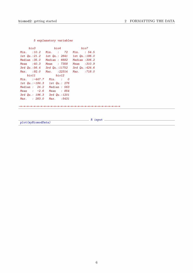
5 explanatory variables
bio3 bio4 bio7
Min. :10.2 Min. : 72 Min. : 54.5
1st Qu.:21.2 1st Qu.: 2641 1st Qu.:186.0
Median :35.0 Median : 6682 Median :306.2
Mean :40.3 Mean : 7358 Mean :310.9
3rd Qu.:56.4 3rd Qu.:11752 3rd Qu.:424.6
Max. :92.0 Max. :22314 Max. :718.0
bio11 bio12
Min. :-447.7 Min. : 0
1st Qu.:-184.3 1st Qu.: 276
Median : 24.2 Median : 563
Mean : -2.6 Mean : 854
3rd Qu.: 196.3 3rd Qu.:1201
Max. : 283.0 Max. :5431
-=-=-=-=-=-=-=-=-=-=-=-=-=-=-=-=-=-=-=-=-=-=-=-=-=-=-=-=-=-=
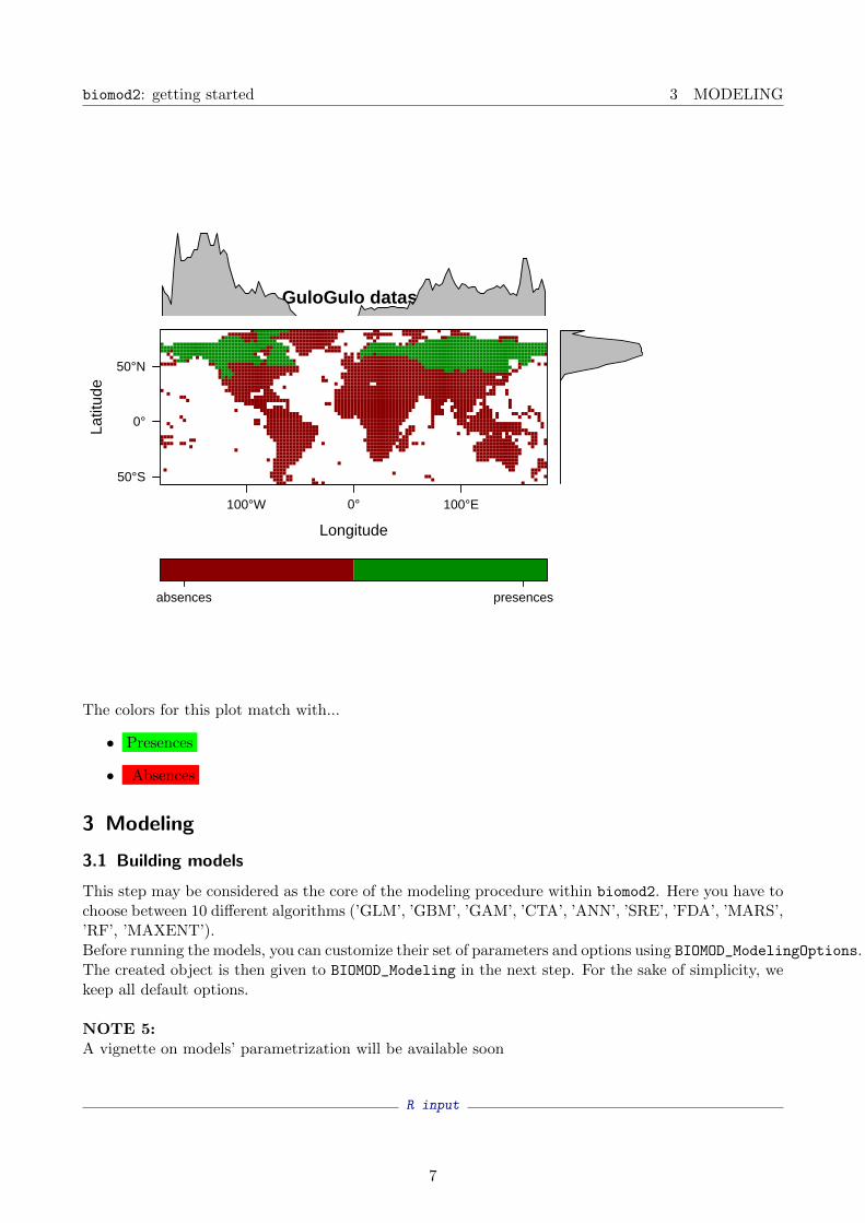
R inputplot(myBiomodData)
6
biomod2: getting started 3 MODELING
GuloGulo datasets
Longitude
Latit
ude
50°S
0°
50°N
100°W 0° 100°E
absences presences
The colors for this plot match with...
• Presences
• Absences
3 Modeling
3.1 Building models
This step may be considered as the core of the modeling procedure within biomod2. Here you have tochoose between 10 different algorithms (’GLM’, ’GBM’, ’GAM’, ’CTA’, ’ANN’, ’SRE’, ’FDA’, ’MARS’,’RF’, ’MAXENT’).Before running the models, you can customize their set of parameters and options using BIOMOD_ModelingOptions.The created object is then given to BIOMOD_Modeling in the next step. For the sake of simplicity, wekeep all default options.
NOTE 5:A vignette on models’ parametrization will be available soon
R input
7
biomod2: getting started 3 MODELING
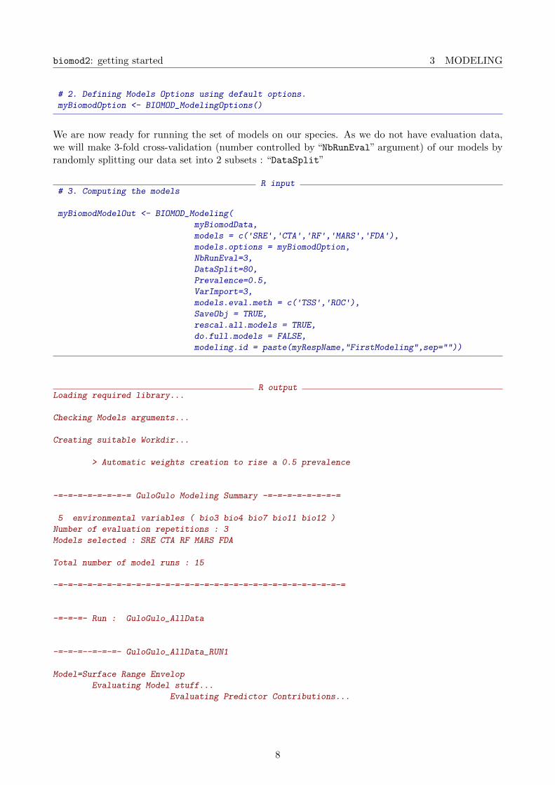
# 2. Defining Models Options using default options.
myBiomodOption <- BIOMOD_ModelingOptions()
We are now ready for running the set of models on our species. As we do not have evaluation data,we will make 3-fold cross-validation (number controlled by “NbRunEval” argument) of our models byrandomly splitting our data set into 2 subsets : “DataSplit”
R input# 3. Computing the models
myBiomodModelOut <- BIOMOD_Modeling(
myBiomodData,
models = c('SRE','CTA','RF','MARS','FDA'),models.options = myBiomodOption,
NbRunEval=3,
DataSplit=80,
Prevalence=0.5,
VarImport=3,
models.eval.meth = c('TSS','ROC'),SaveObj = TRUE,
rescal.all.models = TRUE,
do.full.models = FALSE,
modeling.id = paste(myRespName,"FirstModeling",sep=""))
R outputLoading required library...
Checking Models arguments...
Creating suitable Workdir...
> Automatic weights creation to rise a 0.5 prevalence
-=-=-=-=-=-=-=-= GuloGulo Modeling Summary -=-=-=-=-=-=-=-=
5 environmental variables ( bio3 bio4 bio7 bio11 bio12 )
Number of evaluation repetitions : 3
Models selected : SRE CTA RF MARS FDA
Total number of model runs : 15
-=-=-=-=-=-=-=-=-=-=-=-=-=-=-=-=-=-=-=-=-=-=-=-=-=-=-=-=-=-=
-=-=-=- Run : GuloGulo_AllData
-=-=-=--=-=-=- GuloGulo_AllData_RUN1
Model=Surface Range Envelop
Evaluating Model stuff...
Evaluating Predictor Contributions...
8

biomod2: getting started 3 MODELING
Model=Classification tree
5 Fold Cross-Validation
Model scaling...
Evaluating Model stuff...
Evaluating Predictor Contributions...
Model=Breiman and Cutler's random forests for classification and regression
Model scaling...
Evaluating Model stuff...
Evaluating Predictor Contributions...
Model=Multiple Adaptive Regression Splines
Model scaling...
Evaluating Model stuff...
Evaluating Predictor Contributions...
Model=Flexible Discriminant Analysis
Model scaling...
Evaluating Model stuff...
Evaluating Predictor Contributions...
-=-=-=--=-=-=- GuloGulo_AllData_RUN2
Model=Surface Range Envelop
Evaluating Model stuff...
Evaluating Predictor Contributions...
Model=Classification tree
5 Fold Cross-Validation
Model scaling...
Evaluating Model stuff...
Evaluating Predictor Contributions...
Model=Breiman and Cutler's random forests for classification and regression
Model scaling...
Evaluating Model stuff...
Evaluating Predictor Contributions...
Model=Multiple Adaptive Regression Splines
Model scaling...
Evaluating Model stuff...
Evaluating Predictor Contributions...
Model=Flexible Discriminant Analysis
Model scaling...
Evaluating Model stuff...
Evaluating Predictor Contributions...
-=-=-=--=-=-=- GuloGulo_AllData_RUN3
Model=Surface Range Envelop
Evaluating Model stuff...
Evaluating Predictor Contributions...
9

biomod2: getting started 3 MODELING
Model=Classification tree
5 Fold Cross-Validation
Model scaling...
Evaluating Model stuff...
Evaluating Predictor Contributions...
Model=Breiman and Cutler's random forests for classification and regression
Model scaling...
Evaluating Model stuff...
Evaluating Predictor Contributions...
Model=Multiple Adaptive Regression Splines
Model scaling...
Evaluating Model stuff...
Evaluating Predictor Contributions...
Model=Flexible Discriminant Analysis
Model scaling...
Evaluating Model stuff...
Evaluating Predictor Contributions...
-=-=-=-=-=-=-=-=-=-=-=-=-=-= Done -=-=-=-=-=-=-=-=-=-=-=-=-=-=
R input
When this step is over, have a look at some outputs :
• modeling summary
R inputmyBiomodModelOut
R output-=-=-=-=-=-=-=-=-=-= BIOMOD.models.out -=-=-=-=-=-=-=-=-=-=
Modeling id : GuloGuloFirstModeling
Species modeled : GuloGulo
Considered variables : bio3 bio4 bio7 bio11 bio12
Computed Models : GuloGulo_AllData_RUN1_SRE
GuloGulo_AllData_RUN1_CTA GuloGulo_AllData_RUN1_RF
GuloGulo_AllData_RUN1_MARS GuloGulo_AllData_RUN1_FDA
GuloGulo_AllData_RUN2_SRE GuloGulo_AllData_RUN2_CTA
GuloGulo_AllData_RUN2_RF GuloGulo_AllData_RUN2_MARS
GuloGulo_AllData_RUN2_FDA GuloGulo_AllData_RUN3_SRE
GuloGulo_AllData_RUN3_CTA GuloGulo_AllData_RUN3_RF
GuloGulo_AllData_RUN3_MARS GuloGulo_AllData_RUN3_FDA
Failed Models : none
-=-=-=-=-=-=-=-=-=-=-=-=-=-=-=-=-=-=-=-=-=-=-=-=-=-=-=-=-=-=
10
biomod2: getting started 3 MODELING
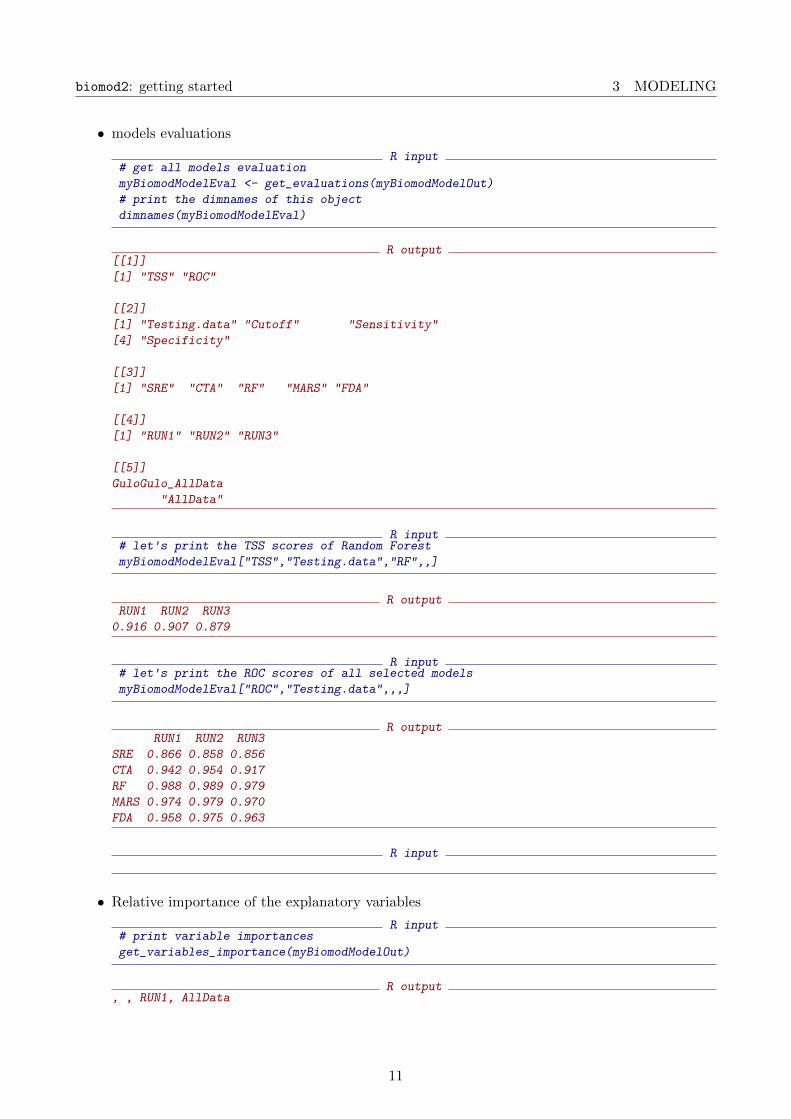
• models evaluations
R input# get all models evaluation
myBiomodModelEval <- get_evaluations(myBiomodModelOut)
# print the dimnames of this object
dimnames(myBiomodModelEval)
R output[[1]]
[1] "TSS" "ROC"
[[2]]
[1] "Testing.data" "Cutoff" "Sensitivity"
[4] "Specificity"
[[3]]
[1] "SRE" "CTA" "RF" "MARS" "FDA"
[[4]]
[1] "RUN1" "RUN2" "RUN3"
[[5]]
GuloGulo_AllData
"AllData"
R input# let's print the TSS scores of Random Forest
myBiomodModelEval["TSS","Testing.data","RF",,]
R outputRUN1 RUN2 RUN3
0.916 0.907 0.879
R input# let's print the ROC scores of all selected models
myBiomodModelEval["ROC","Testing.data",,,]
R outputRUN1 RUN2 RUN3
SRE 0.866 0.858 0.856
CTA 0.942 0.954 0.917
RF 0.988 0.989 0.979
MARS 0.974 0.979 0.970
FDA 0.958 0.975 0.963
R input
• Relative importance of the explanatory variables
R input# print variable importances
get_variables_importance(myBiomodModelOut)
R output, , RUN1, AllData
11

biomod2: getting started 3 MODELING
SRE CTA RF MARS FDA
Var1 0.388 0.285 0.165 0.358 0.257
Var2 0.380 0.285 0.164 0.356 0.252
Var3 0.370 0.285 0.167 0.360 0.256
, , RUN2, AllData
SRE CTA RF MARS FDA
Var1 0.383 0.331 0.170 0.351 0.268
Var2 0.375 0.331 0.166 0.349 0.273
Var3 0.378 0.331 0.171 0.341 0.269
, , RUN3, AllData
SRE CTA RF MARS FDA
Var1 0.364 0.317 0.159 0.384 0.275
Var2 0.372 0.317 0.159 0.405 0.270
Var3 0.378 0.317 0.165 0.390 0.276
NOTE 6:Relative importance of variable returned are raw data. It may be usefull to normalise them tomake them comparable one to another
3.2 Ensemble modeling
Here comes one of the most interesting features of biomod2. BIOMOD_EnsembleModeling combinesindividual models to build some kind of meta-model. In the following example, we decide to excludeall models having a TSS score lower than 0.7.
NOTE 7:You can controle the way formal models are combined with em.by argument. The vignette ”Ensem-bleModelingAssembly” illustrate the offered possibilities
R inputmyBiomodEM <- BIOMOD_EnsembleModeling(
modeling.output = myBiomodModelOut,
chosen.models = 'all',em.by='all',eval.metric = c('TSS'),eval.metric.quality.threshold = c(0.7),
prob.mean = T,
prob.cv = T,
prob.ci = T,
prob.ci.alpha = 0.05,
prob.median = T,
committee.averaging = T,
prob.mean.weight = T,
prob.mean.weight.decay = 'proportional' )
12

biomod2: getting started 3 MODELING
R output-=-=-=-=-=-=-=-=-= Build Ensemble Models -=-=-=-=-=-=-=-=-=
! all models available will be included in ensemble.modeling
> Evaluation & Weighting methods summary :
TSS over 0.7
> TotalConsensus ensemble modeling
! Models projections for whole zonation required...
> Projecting GuloGulo_AllData_RUN1_SRE ...
> Projecting GuloGulo_AllData_RUN1_CTA ...
> Projecting GuloGulo_AllData_RUN1_RF ...
> Projecting GuloGulo_AllData_RUN1_MARS ...
> Projecting GuloGulo_AllData_RUN1_FDA ...
> Projecting GuloGulo_AllData_RUN2_SRE ...
> Projecting GuloGulo_AllData_RUN2_CTA ...
> Projecting GuloGulo_AllData_RUN2_RF ...
> Projecting GuloGulo_AllData_RUN2_MARS ...
> Projecting GuloGulo_AllData_RUN2_FDA ...
> Projecting GuloGulo_AllData_RUN3_SRE ...
> Projecting GuloGulo_AllData_RUN3_CTA ...
> Projecting GuloGulo_AllData_RUN3_RF ...
> Projecting GuloGulo_AllData_RUN3_MARS ...
> Projecting GuloGulo_AllData_RUN3_FDA ...
> Mean of probabilities...
Evaluating Model stuff...
> Coef of variation of probabilities...
Evaluating Model stuff...
> Confidence Interval...
Evaluating Model stuff...
Evaluating Model stuff...
> Median of ptobabilities...
Evaluating Model stuff...
> Comittee averaging...
Evaluating Model stuff...
> Prababilities wegthing mean...
Evaluating Model stuff...
-=-=-=-=-=-=-=-=-=-=-=-=-=-= Done -=-=-=-=-=-=-=-=-=-=-=-=-=-=
You can easily access to the data and outputs of BIOMOD_Modeling using some specific functions tomake your life easier.Let’s see the meta-models evaluation scores.
NOTE 8:We decide to evaluate all meta-models produced even the CV (Coefficient of Variation) one which isquite hard to interpret. You may consider it as: higher my score is, more the variation is localisedwhere my species is forecasted as present.
R input# print summary
myBiomodEM
13
biomod2: getting started 4 PROJECTION
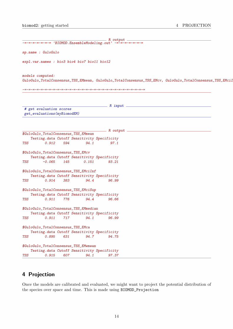
R output-=-=-=-=-=-=-= 'BIOMOD.EnsembleModeling.out' -=-=-=-=-=-=-=
sp.name : GuloGulo
expl.var.names : bio3 bio4 bio7 bio11 bio12
models computed:
GuloGulo_TotalConsensus_TSS_EMmean, GuloGulo_TotalConsensus_TSS_EMcv, GuloGulo_TotalConsensus_TSS_EMciInf, GuloGulo_TotalConsensus_TSS_EMciSup, GuloGulo_TotalConsensus_TSS_EMmedian, GuloGulo_TotalConsensus_TSS_EMca, GuloGulo_TotalConsensus_TSS_EMwmean
-=-=-=-=-=-=-=-=-=-=-=-=-=-=-=-=-=-=-=-=-=-=-=-=-=-=-=-=-=-=
R input# get evaluation scores
get_evaluations(myBiomodEM)
R output$GuloGulo_TotalConsensus_TSS_EMmean
Testing.data Cutoff Sensitivity Specificity
TSS 0.912 594 94.1 97.1
$GuloGulo_TotalConsensus_TSS_EMcv
Testing.data Cutoff Sensitivity Specificity
TSS -0.065 145 0.151 93.21
$GuloGulo_TotalConsensus_TSS_EMciInf
Testing.data Cutoff Sensitivity Specificity
TSS 0.914 383 94.4 96.99
$GuloGulo_TotalConsensus_TSS_EMciSup
Testing.data Cutoff Sensitivity Specificity
TSS 0.911 776 94.4 96.66
$GuloGulo_TotalConsensus_TSS_EMmedian
Testing.data Cutoff Sensitivity Specificity
TSS 0.911 717 94.1 96.99
$GuloGulo_TotalConsensus_TSS_EMca
Testing.data Cutoff Sensitivity Specificity
TSS 0.895 631 94.7 94.75
$GuloGulo_TotalConsensus_TSS_EMwmean
Testing.data Cutoff Sensitivity Specificity
TSS 0.915 607 94.1 97.37
4 Projection
Once the models are calibrated and evaluated, we might want to project the potential distribution ofthe species over space and time. This is made using BIOMOD_Projection
14

biomod2: getting started 4 PROJECTION
NOTE 9:All projections are stored directly on your hard drive
First let’s project the individual models on our current conditions (the globe) to visualize them.
R input# projection over the globe under current conditions
myBiomodProj <- BIOMOD_Projection(
modeling.output = myBiomodModelOut,
new.env = myExpl,
proj.name = 'current',selected.models = 'all',binary.meth = 'TSS',compress = 'xz',clamping.mask = F,
output.format = '.grd')
R output-=-=-=-=-=-=-=-=-= Do Models Projections -=-=-=-=-=-=-=-=-=
> Building clamping mask
> Projecting GuloGulo_AllData_RUN1_SRE ...
> Projecting GuloGulo_AllData_RUN1_CTA ...
> Projecting GuloGulo_AllData_RUN1_RF ...
> Projecting GuloGulo_AllData_RUN1_MARS ...
> Projecting GuloGulo_AllData_RUN1_FDA ...
> Projecting GuloGulo_AllData_RUN2_SRE ...
> Projecting GuloGulo_AllData_RUN2_CTA ...
> Projecting GuloGulo_AllData_RUN2_RF ...
> Projecting GuloGulo_AllData_RUN2_MARS ...
> Projecting GuloGulo_AllData_RUN2_FDA ...
> Projecting GuloGulo_AllData_RUN3_SRE ...
> Projecting GuloGulo_AllData_RUN3_CTA ...
> Projecting GuloGulo_AllData_RUN3_RF ...
> Projecting GuloGulo_AllData_RUN3_MARS ...
> Projecting GuloGulo_AllData_RUN3_FDA ...
> Building TSS binaries
-=-=-=-=-=-=-=-=-=-=-=-=-=-= Done -=-=-=-=-=-=-=-=-=-=-=-=-=-=
R input# summary of crated oject
myBiomodProj
R output-=-=-=-=-=-=-=-=-= 'BIOMOD.projection.out' -=-=-=-=-=-=-=-=-=
Projection directory : GuloGulo/current
sp.name : GuloGulo
15
biomod2: getting started 4 PROJECTION
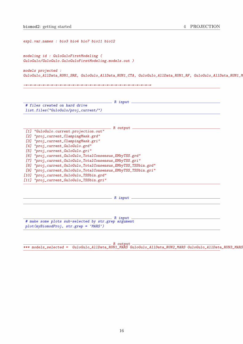
expl.var.names : bio3 bio4 bio7 bio11 bio12
modeling id : GuloGuloFirstModeling (
GuloGulo/GuloGulo.GuloGuloFirstModeling.models.out )
models projected :
GuloGulo_AllData_RUN1_SRE, GuloGulo_AllData_RUN1_CTA, GuloGulo_AllData_RUN1_RF, GuloGulo_AllData_RUN1_MARS, GuloGulo_AllData_RUN1_FDA, GuloGulo_AllData_RUN2_SRE, GuloGulo_AllData_RUN2_CTA, GuloGulo_AllData_RUN2_RF, GuloGulo_AllData_RUN2_MARS, GuloGulo_AllData_RUN2_FDA, GuloGulo_AllData_RUN3_SRE, GuloGulo_AllData_RUN3_CTA, GuloGulo_AllData_RUN3_RF, GuloGulo_AllData_RUN3_MARS, GuloGulo_AllData_RUN3_FDA
-=-=-=-=-=-=-=-=-=-=-=-=-=-=-=-=-=-=-=-=-=-=-=-=-=-=-=-=-=-=
R input# files created on hard drive
list.files("GuloGulo/proj_current/")
R output[1] "GuloGulo.current.projection.out"
[2] "proj_current_ClampingMask.grd"
[3] "proj_current_ClampingMask.gri"
[4] "proj_current_GuloGulo.grd"
[5] "proj_current_GuloGulo.gri"
[6] "proj_current_GuloGulo_TotalConsensus_EMbyTSS.grd"
[7] "proj_current_GuloGulo_TotalConsensus_EMbyTSS.gri"
[8] "proj_current_GuloGulo_TotalConsensus_EMbyTSS_TSSbin.grd"
[9] "proj_current_GuloGulo_TotalConsensus_EMbyTSS_TSSbin.gri"
[10] "proj_current_GuloGulo_TSSbin.grd"
[11] "proj_current_GuloGulo_TSSbin.gri"
R input
R input# make some plots sub-selected by str.grep argument
plot(myBiomodProj, str.grep = 'MARS')
R output*** models_selected = GuloGulo_AllData_RUN1_MARS GuloGulo_AllData_RUN2_MARS GuloGulo_AllData_RUN3_MARS
16

biomod2: getting started 4 PROJECTION
GuloGulo current projections
Longitude
Latit
ude
50°S
0°
50°N
GuloGulo_AllData_RUN1_MARS
GuloGulo_AllData_RUN2_MARS
50°S
0°
50°N
100°W 0° 100°E
GuloGulo_AllData_RUN3_MARS
0
250
500
750
1000
R input# if you want to make custom plots, you can also get the projected map
myCurrentProj <- get_predictions(myBiomodProj)
R output*** models_selected = GuloGulo_AllData_RUN1_SRE GuloGulo_AllData_RUN1_CTA GuloGulo_AllData_RUN1_RF GuloGulo_AllData_RUN1_MARS GuloGulo_AllData_RUN1_FDA GuloGulo_AllData_RUN2_SRE GuloGulo_AllData_RUN2_CTA GuloGulo_AllData_RUN2_RF GuloGulo_AllData_RUN2_MARS GuloGulo_AllData_RUN2_FDA GuloGulo_AllData_RUN3_SRE GuloGulo_AllData_RUN3_CTA GuloGulo_AllData_RUN3_RF GuloGulo_AllData_RUN3_MARS GuloGulo_AllData_RUN3_FDA
R inputmyCurrentProj
R outputclass : RasterStack
dimensions : 47, 120, 5640, 15 (nrow, ncol, ncell, nlayers)
resolution : 3, 3 (x, y)
extent : -180, 180, -57.5, 83.5 (xmin, xmax, ymin, ymax)
coord. ref. : +proj=longlat +datum=WGS84 +no_defs +ellps=WGS84 +towgs84=0,0,0
names : GuloGulo_AllData_RUN1_SRE, GuloGulo_AllData_RUN1_CTA, GuloGulo_AllData_RUN1_RF, GuloGulo_AllData_RUN1_MARS, GuloGulo_AllData_RUN1_FDA, GuloGulo_AllData_RUN2_SRE, GuloGulo_AllData_RUN2_CTA, GuloGulo_AllData_RUN2_RF, GuloGulo_AllData_RUN2_MARS, GuloGulo_AllData_RUN2_FDA, GuloGulo_AllData_RUN3_SRE, GuloGulo_AllData_RUN3_CTA, GuloGulo_AllData_RUN3_RF, GuloGulo_AllData_RUN3_MARS, GuloGulo_AllData_RUN3_FDA
min values : 0, 18, 3, 0, 164, 0, 17, 3, 0, 140, 0, 30, 7, 0, 151
max values : 1000, 946, 1000, 1000, 996, 1000, 976, 1000, 1000, 997, 1000, 974, 1000, 1000, 997
17

biomod2: getting started 4 PROJECTION
Then we can project the potential distribution of the species over time, i.e. into the future.
R input# load environmental variables for the future.
myExplFuture = stack( system.file( "external/bioclim/future/bio3.grd",
package="biomod2"),
system.file( "external/bioclim/future/bio4.grd",
package="biomod2"),
system.file( "external/bioclim/future/bio7.grd",
package="biomod2"),
system.file( "external/bioclim/future/bio11.grd",
package="biomod2"),
system.file( "external/bioclim/future/bio12.grd",
package="biomod2"))
myBiomodProjFuture <- BIOMOD_Projection(
modeling.output = myBiomodModelOut,
new.env = myExplFuture,
proj.name = 'future',selected.models = 'all',binary.meth = 'TSS',compress = 'xz',clamping.mask = T,
output.format = '.grd')
R output-=-=-=-=-=-=-=-=-= Do Models Projections -=-=-=-=-=-=-=-=-=
> Building clamping mask
> Projecting GuloGulo_AllData_RUN1_SRE ...
> Projecting GuloGulo_AllData_RUN1_CTA ...
> Projecting GuloGulo_AllData_RUN1_RF ...
> Projecting GuloGulo_AllData_RUN1_MARS ...
> Projecting GuloGulo_AllData_RUN1_FDA ...
> Projecting GuloGulo_AllData_RUN2_SRE ...
> Projecting GuloGulo_AllData_RUN2_CTA ...
> Projecting GuloGulo_AllData_RUN2_RF ...
> Projecting GuloGulo_AllData_RUN2_MARS ...
> Projecting GuloGulo_AllData_RUN2_FDA ...
> Projecting GuloGulo_AllData_RUN3_SRE ...
> Projecting GuloGulo_AllData_RUN3_CTA ...
> Projecting GuloGulo_AllData_RUN3_RF ...
> Projecting GuloGulo_AllData_RUN3_MARS ...
> Projecting GuloGulo_AllData_RUN3_FDA ...
> Building TSS binaries
-=-=-=-=-=-=-=-=-=-=-=-=-=-= Done -=-=-=-=-=-=-=-=-=-=-=-=-=-=
R input
R input# make some plots, sub-selected by str.grep argument
plot(myBiomodProjFuture, str.grep = 'MARS')
18

biomod2: getting started 4 PROJECTION
R output*** models_selected = GuloGulo_AllData_RUN1_MARS GuloGulo_AllData_RUN2_MARS GuloGulo_AllData_RUN3_MARS
GuloGulo future projections
Longitude
Latit
ude
50°S
0°
50°N
GuloGulo_AllData_RUN1_MARS
GuloGulo_AllData_RUN2_MARS
50°S
0°
50°N
100°W 0° 100°E
GuloGulo_AllData_RUN3_MARS
0
250
500
750
1000
The last step of this vignette is to make Ensemble Forcasting, that means to project the meta-models you have created with BIOMOD_EnsembleModeling. BIOMOD_EnsembleForecasting requiredthe output of BIOMOD_EnsembleModeling and BIOMOD_Projection. It will combine the projectionsmade according to models ensemble rules defined at the ensemble modelling step.
R inputmyBiomodEF <- BIOMOD_EnsembleForecasting(
EM.output = myBiomodEM,
projection.output = myBiomodProj)
R output-=-=-=-=-=-=-= Do Ensemble Models Projections -=-=-=-=-=-=-=
*** models_selected = GuloGulo_AllData_RUN1_SRE GuloGulo_AllData_RUN1_CTA GuloGulo_AllData_RUN1_RF GuloGulo_AllData_RUN1_MARS GuloGulo_AllData_RUN1_FDA GuloGulo_AllData_RUN2_SRE GuloGulo_AllData_RUN2_CTA GuloGulo_AllData_RUN2_RF GuloGulo_AllData_RUN2_MARS GuloGulo_AllData_RUN2_FDA GuloGulo_AllData_RUN3_SRE GuloGulo_AllData_RUN3_CTA GuloGulo_AllData_RUN3_RF GuloGulo_AllData_RUN3_MARS GuloGulo_AllData_RUN3_FDA
> Projecting GuloGulo_TotalConsensus_TSS_EMmean ...
> Projecting GuloGulo_TotalConsensus_TSS_EMcv ...
> Projecting GuloGulo_TotalConsensus_TSS_EMciInf ...
19

biomod2: getting started 4 PROJECTION
> Projecting GuloGulo_TotalConsensus_TSS_EMciSup ...
> Projecting GuloGulo_TotalConsensus_TSS_EMmedian ...
> Projecting GuloGulo_TotalConsensus_TSS_EMca ...
> Projecting GuloGulo_TotalConsensus_TSS_EMwmean ...
-=-=-=-=-=-=-=-=-=-=-=-=-=-= Done -=-=-=-=-=-=-=-=-=-=-=-=-=-=
Object return has the same type than ones returned by BIOMOD_Projection. Moreover some addi-tional files have been created in your projection folder (“RasterStack” or “array” depending on yourprojection type). This file contains your meta-models projections.
R inputmyBiomodEF
R output-=-=-=-=-=-=-=-=-= 'BIOMOD.projection.out' -=-=-=-=-=-=-=-=-=
Projection directory : GuloGulo/current
sp.name : GuloGulo
expl.var.names : bio3 bio4 bio7 bio11 bio12
modeling id : GuloGuloFirstModeling (
GuloGulo/GuloGulo.GuloGuloFirstModeling.models.out )
models projected :
GuloGulo_TotalConsensus_TSS_EMmean, GuloGulo_TotalConsensus_TSS_EMcv, GuloGulo_TotalConsensus_TSS_EMciInf, GuloGulo_TotalConsensus_TSS_EMciSup, GuloGulo_TotalConsensus_TSS_EMmedian, GuloGulo_TotalConsensus_TSS_EMca, GuloGulo_TotalConsensus_TSS_EMwmean
-=-=-=-=-=-=-=-=-=-=-=-=-=-=-=-=-=-=-=-=-=-=-=-=-=-=-=-=-=-=
R input# reduce layer names for plotting convegences
plot(myBiomodEF)
R output*** models_selected = GuloGulo_TotalConsensus_TSS_EMmean GuloGulo_TotalConsensus_TSS_EMcv GuloGulo_TotalConsensus_TSS_EMciInf GuloGulo_TotalConsensus_TSS_EMciSup GuloGulo_TotalConsensus_TSS_EMmedian GuloGulo_TotalConsensus_TSS_EMca GuloGulo_TotalConsensus_TSS_EMwmean
20

biomod2: getting started 5 CONCLUSION
GuloGulo current projections
Longitude
Latit
ude
50°S
0°
50°N
GuloGulo_TotalConsensus_TSS_EMmeanGuloGulo_TotalConsensus_TSS_EMcv
GuloGulo_TotalConsensus_TSS_EMciInfGuloGulo_TotalConsensus_TSS_EMciSup
50°S
0°
50°N
GuloGulo_TotalConsensus_TSS_EMmedianGuloGulo_TotalConsensus_TSS_EMca
100°W 0° 100°E
GuloGulo_TotalConsensus_TSS_EMwmean
0
250
500
750
1000
5 Conclusion
This vignette describes how to build and test a range of models within biomod2 but also how to buildensemble projections under current and future conditions. With few modifications, you should be ableto apply the default functions onto your own dataset.
21