Western Kentucky UniversityTopSCHOLAR®

Masters Theses & Specialist Projects Graduate School

8-2012

An Examination of White-Nose SyndromeOccurrence and Dispersal Patterns: UtilizingGlobal and Local Moran's I Analysis to Evaluate anEmerging PathogenCelia M. DavisWestern Kentucky University, celia.davis162@topper.wku.edu

Follow this and additional works at: http://digitalcommons.wku.edu/theses

Part of the Environmental Health and Protection Commons

This Thesis is brought to you for free and open access by TopSCHOLAR®. It has been accepted for inclusion in Masters Theses & Specialist Projects byan authorized administrator of TopSCHOLAR®. For more information, please contact topscholar@wku.edu.

Recommended CitationDavis, Celia M., "An Examination of White-Nose Syndrome Occurrence and Dispersal Patterns: Utilizing Global and Local Moran's IAnalysis to Evaluate an Emerging Pathogen" (2012). Masters Theses & Specialist Projects. Paper 1194.http://digitalcommons.wku.edu/theses/1194

 

 

AN EXAMINATION OF WHITE-NOSE SYNDROME OCCURRENCE AND DISPERSAL PATTERNS: UTILIZING GLOBAL AND LOCAL MORAN’S I

ANALYSIS TO EVALUATE AN EMERGING PATHOGEN

A Thesis Presented to

The Faculty of the Geography and Geology Department Western Kentucky University

Bowling Green, Kentucky

In Partial Fulfillment Of the Requirements for the Degree

Master of Science

By Celia M. Davis

August 2012

iii 

ACKNOWLEDGMENTS Many thanks to the numerous researchers and agencies instrumental in providing

the White-Nose Syndrome confirmation dates that made this research possible and whose

thoughtful critiques were intrinsic to its development. Particular thanks are due to Cal

Butchkoski with the Pennsylvania Game Commission and Carl Herzog with the New

York State Department of Conservation for their assistance in assembling the final

dataset and invaluable input to the project. Thanks are also due to Dr. Jason Polk and Dr.

Rick Toomey at Western Kentucky University for their tremendous input in the design,

implementation, and realization of this project. As always, my eternal gratitude goes out

to Pima, Tassie, Tupelo, and the Davis clan for their moral and financial support and

patience.

iv 

TABLE OF CONTENTS

LIST OF ILLUSTRATIONS……………………………….…………………...…..... v

ABSTRACT..………………………………………………..………………………... vi

INTRODUCTION ………………………………………………………..…………. 1

LITERATURE REVIEW...……………………………….………...…....................... 5

METHODS...……………………………….………...………………………………. 11

RESULTS…………………………….…………………..…….................................. 15

DISCUSSION...……………………………………….……………………………... 22

APPENDIX: Geomyces destructans Confirmation Date...………………………….. 31

REFEREENCES....………………………………………………………..………...... 35

v 

LIST OF ILLUSTRATIONS

Equation 1 Local Moran’s I …………...…………..………………………….……. 13

Figure 1 Frequency Distribution of Month Data………………..…………….......... 14

Figure 2 Spatial Autocorrelation Report, Global Moran’s I....…………….….……. 16

Figure 3 Local Moran’s I p-scores……………………………………….…..……... 17

Figure 4 Local Moran’s I CO-type………………….…….…………………....…… 18

Figure 5 Spatial Autocorrelation Report, Global Moran’s I Variable Date………… 19

Figure 6 Local Moran’s I CO-type, Variable Date…………………………………. 20

Figure 7 Local Moran’s I p-scores, Variable Date……………....………..…….….. 21

vi 

AN EXAMINATION OF WHITE-NOSE SYNDROME OCCURRENCE AND DISPERSAL PATTERNS: UTILIZING GLOBAL AND LOCAL MORAN’S I

ANALYSIS TO EVALUATE AN EMERGING PATHOGEN

Celia M. Davis August 2012 38 Pages

Directed By: Dr. Jason Polk, Dr. Chris Groves, Dr. Jun Yan, and Dr. Rickard Toomey

Department of Geography and Geology Western Kentucky University

In this research, a novel approach that utilizes Moran’s I statistical analyses to

examine the spatio-temporal dispersal patterns of the White-Nose Syndrome currently

affecting North American bat species is undertaken to further understand the disease

transmission mechanism(s) of this emerging wildlife epidemic. White-Nose Syndrome

has been responsible for in excess of five million bat deaths to date and has the potential

to alter the ecological landscape significantly; however, due to a variety of factors, little

research has been conducted into the patterns of infection on a national scale. Global and

Local Moran’s I analyses were performed on the spatial-temporal variable of month and

location from the initial outbreak site in order to address the spread of the Geomyces

destructans fungus that causes White-Nose Syndrome. A comprehensive dataset of

outbreak confirmation sites has been compiled and statistical analysis using ArcGIS

reveals a complex pattern of disease dispersion since initial discovery of the disease, and

shows important policy and management implications, in particular the need for more

standardized and rigorous data collection and reporting procedures.

1

Introduction

The small blue-green planet on which we live is a closed system and, within this

closed system, each component part has its role to play in the continued functioning of

the whole. The demands human beings place on the myriad interdependent eco-systems

that surround and envelop us have far-reaching implications not only for our own

survival, but for the almost infinite number of plant and animal species upon which we

depend for the most basic of necessities. As global population growth continues

unchecked, the rate at which finite natural resources are being consumed becomes an

almost exponential equation, and anthropogenic consequences are the inevitable end-

result. In light of this disturbing trend, it seems self-evident that any developments

having the potential to disrupt or diminish existing agricultural production should be of

great concern.

Worldwide population growth and an increasing standard of living in the United

States place an unprecedented strain on available food resources for both domestic

consumption and global export. The Food and Agriculture Organization of the United

Nations estimates that in the past year alone the global economic crisis and continued

population expansion will cause approximately 1.02 billion world citizens to be

undernourished (FAO, 2009). American farmers and agri-business companies meet this

increased demand in food production in a variety of ways, resulting in the use of higher

yield genetically modified crops, increased pesticide usage, and alterations in crop-

growing methods. A significant concern is that pesticide applications have long been

linked to undesirable side-effects, such as contamination of the water table, along with

severe short-term and long-term risks to humans directly exposed to the chemicals

2

currently available for crop pest control. Along with the costs (both financial and human-

health related) of extensive pesticide use, there is also a well-demonstrated tendency for

natural pests to develop resistance to chemicals over ever-shorter periods of time. In

light of these significant drawbacks to the use of chemicals in controlling the populations

of crop-destroying pests, it is imperative to continue research into alternative schemes to

reduce dependence on chemical pesticides.

The concept of “keystone” species is not novel, and the wide-spread attention

drawn to serious population declines of the American honey bee and amphibian species

in the latter half of the twentieth century indicates a dawning awareness on the part of the

scientific community that the demands being placed on this closed system have

consequences (Meteyer et al., 2000; Johnson, 2007). These consequences may not be

readily apparent to the average world citizen; nevertheless, the decimation of seemingly

peripheral species should serve as a warning that all is not well. In the same way other

species as diverse as bees and frogs have sounded this warning, bats also function as bio-

indicators for the environments surrounding their various species (Jones et al., 2009). As

in most cases of this sort, the connections between human activities and broad-ranging

declines amongst the flora and fauna surrounding person-kind are complex, nuanced, and

multi-faceted.

Over time, nature has evolved a system of checks and balances between predator

species and the insect populations that target the most prominent food crops grown

domestically. In the case of corn, soybeans, wheat, and rice, a great number of bird and

bat species have developed into extremely effective ‘bug killing machines.’ It is a well-

documented fact that individual North American bats readily devour up to 2000 insects

3

each night and crops without these nightly visits show over a 150% increase in pest load

(Kalka et al., 2008). In addition to feasting on specific crop pests, bats are also believed

responsible for significant control of mosquito populations in states like Texas and

Florida, where millions of dollars are spent annually in efforts to control the spread of

West Nile Disease (Cleveland et al., 2006). Given the financial and environmental

impact of controlling insect populations by chemical means, it should be of particular

concern when an emerging infectious disease decimates over 90% of affected bat

populations and results in an even greater use of pesticides that eventually make their

way downstream into the environment (Blehert et al., 2009).

The so-called “White-Nose Syndrome,” where bat populations affected by the

Geomyces destructans fungus leave hibernation early and experience high mortality rates

due to insufficient wintertime food resources, has become rampant along the eastern

seaboard since its initial discovery in Albany, NY in 2006 (Blehert et al., 2009), and

confirmation of the fungus itself being present occurred as far west as Missouri (Wibbelt

et al., 2010) and Oklahoma, although there is no report of resulting mortality in those

western-most states as of now.

Since its initial discovery in Howe’s Cave outside Albany, New York in the latter

months of 2006 and subsequent confirmation in March of 2007, White-Nosed Syndrome

(WNS) and its causative Geomyces destructans fungus have been responsible for

decimating populations of Myotis Lucifugus (Little Brown bats) and Myotis sodalis (the

already critically endangered Indiana bat). Based on census numbers from the United

States Fish and Wildlife Service (FWS) and state-level agencies, the trend of mortality is

apparent with greater than 90% declines in populations of both species at surveyed sites

4

and predictive population models indicate regional extinction of Myotis lucifigus within

shockingly short time frames (Frick et al., 2010). Despite intensive efforts underway in

a variety of fields to understand the mechanisms and dispersal factors of WNS,

researchers have yet to conclusively identify the pattern of the disease spread and are thus

significantly handicapped in their attempts to predict where and when the next outbreaks

will occur. This inability to pinpoint even approximate spread patterns leaves state and

federal efforts lacking at being able to mitigate the devastating effects of this disease

upon one of our most economically valuable wildlife groups.

The goal of this project is two-fold; firstly, to gather all existing WNS outbreak

data by county level location and outbreak date at the level of month, and secondly, to

utilize the statistical tools available within the ArcMap GIS software to perform an initial

analysis of the disease dispersion patterns present as of April 2012 in an effort to better

understand the mechanism(s) behind disease dispersion. Should outlier values be yielded

by such a statistical analysis of confirmed WNS sites and their infection dates, it would

be an indication that a host capable of acting as vector to the fungus over significant

distances could be implicated in contributing to the disease dispersal.

5

Literature Review

The full economic impact of bat predation on pest insect populations is poorly

documented; however, studies by Wickramasinghe et al. (2004), Cleveland et al. (2006),

Kalka et al. (2008), and Boyles et al. (2011) indicate that the predatory role of bats on

food pests is considerable. In the case of the Brazilian free-tailed bat, Cleveland et al.

(2006) found that there was a 12% overall decrease in corn crop infestation by larval

worm pests directly attributable to bat predation in south-central Texas. Although studies

have not been conducted to confirm the effect across other parts of the country, this

figure is likely to be similar in states that also have insectivorous bat populations whose

range extends over agricultural areas. Given that insectivorous bat species function as a

natural pest-control mechanism with not insignificant financial and environmental

benefits, the loss of large portions of indigenous bat populations as seen in White-Nose

Syndrome is especially troubling.

The first reports of this mysterious disease that resulted in high bat mortality were

centered at Howe’s Cave of Albany, New York, in the early spring of 2006 (Blehert et

al., 2009) when recreational cavers noticed high numbers of dead bats immediately

outside of the cave. Upon examination by local fish and wildlife employees, it became

apparent that not only was the local population of little brown bats (Myotis lucifugus)

experiencing mortality of greater than 90%, but that significantly abnormal behavior in

flying and feeding patterns was observed in surviving individuals. Losses of greater than

90% were then discovered in nearby hibernacula during winter of 2006-2007 and the

condition rapidly spread along the United States eastern seaboard. As of spring 2012,

nine insectivorous bat species in nineteen states had experienced Geomyces destructans

6

infection (USFWS, July 2012d) and research into the cause of WNS-associated mortality

was well underway. Despite the identification of the Geomyces destructans fungus

responsible for WNS (Lorch et al., 2011), and the physiological symptoms of the

syndrome (Reichard and Kunz, 2009), the exact mechanism of the resulting fatality of

infected individuals is still poorly understood. It is of particular interest that the presence

of bats exhibiting White-Nose fungus symptoms has been well documented in a majority

of European countries with no resulting mortality (Wibbelt et al., 2010). Equally

noteworthy is the correlation existing research has found between body fat ratios and

mortality rates (Geluso et al., 1976; Clark et al., 1983), since metabolic malfunction is

one possible culprit behind White-Nose Syndrome deaths. Starvation after early awaking

from hibernation has been implicated (Turbill and Geiser, 2008; Reichard and Kunz,

2009) and further research speculates that evaporative water loss leading to dehydration

is the motivating force behind early awakening (Cryan et al., 2010; Willis et al., 2011).

Advances in computing power have allowed for increasingly rigorous

investigations of Tobler’s First Law of Geography, which states, “Everything is related to

everything else, but near things are more related than distant things” and this most

fundamental statement of autocorrelation or the reality that, “any set of spatial data is

likely to have characteristic distances or lengths at which is it correlated with itself”

(Sullivan and Unwin, 2003; 180) and can now be readily applied to real world

phenomena. Natural world occurrences, like those of White-Nose Syndrome, can be

analyzed statistically to reveal patterns within the dataset that reflect autocorrelations and

these patterns can be compared to a randomly generated matching dataset to establish the

degree of non-randomness present in the phenomenon being examined.

7

One such analysis that examines spatial autocorrelation across a dataset is the

Moran’s I statistic which is typically applied to areal units that possess interval data

characteristics and compares the relationship of observed data to that of randomly

generated data in order to establish a measure of positive autocorrelation (clustered),

negative autocorrelation (dispersed), or no autocorrelation (random) (O’Sullivan and

Unwin, 2003; 197). Although useful for determining overall patterns of a particular

dataset, the Global Moran’s I statistic falls short when examining the relationships

between sites of that dataset, and this shortcoming was addressed with the development

of a Local Moran’s I analysis that yields further information about where the patterns of

autocorrelation exist within the occurrences of interest (Anselin, 1995). An important

distinction between the analyses is that Local Moran’s I is disaggregate and therefore

examines the degree to which neighboring data points are similar or dissimilar.

Despite the significant volume of research that has been conducted around the

physiological consequences of WNS, characterization of the fungus itself, and controlled

examinations of transmission factors, less emphasis has been placed on understanding the

patterns within the disease dispersal of existing sites. In part, the reluctance to undertake

these sorts of analyses may be due to a perceived lack of tools to address the nature and

scope of the epidemic. However, since the development of ArcGIS’s sophisticated

statistics software package and the inclusion of tests such as Global and Local Moran’s I,

Geary’s Function, K Function, these statistics-driven analyses have been utilized by

numerous researchers from very different fields of study to analyze similar phenomena

and depict results in a concise, visually compelling manner.

8

In their research tracking shigellosis, McKee et al. (2000) employed a simple k-

nearest neighbor calculation to explore infection patterns on a military base at Fort Bragg,

North Carolina and established that the infection is indeed locally contagious. Prior to

the shigellosis research, K-function analysis had also been effectively utilized by

Morrison et al. (1998) in their work with tracking the spatial and chronological analysis

of dengue cases in Florida, Puerto Rico, and this analysis also revealed a distinctive

“hotspot” pattern. To address the shortcomings of k-nearest neighbor analysis, Local

Moran’s I analysis was used by Yeshiwondim et al. (2009) to further explicate spatial

patterns of malaria incidents in Ethiopia and this increasingly rigorous analysis revealed

that the CO-type (cluster/outlier type; referring to high-high, low-low, etc. data)

“outliers” that result from Local Moran’s I analysis do indeed offer a more nuanced,

detailed examination of the phenomenon than that found by nearest neighbor statistics

alone. Another study focused on Dengue fever in Northern Thailand by Nakhapakorna

and Jirakojohnkoolb in 2006 used the more specific Local Moran’s I and Geary’s

analysis available within the ArcMap platform to provide a detailed analysis of outlier

regions within the epidemic study area. Again, this Local Moran’s I analysis was utilized

more recently in research by Sugumaran et al. (2009) that examined the spread and

distribution of West Nile virus incidence in the United States to reveal areas in which

neighboring counties showed significantly different values of viral outbreaks. West Nile

Virus was also the focus of further research utilizing Local Moran’s I analysis to examine

spatial autocorrelations of hotspot activity over time (Carnes and Ogneva-Himmelberger,

2011).

In contrast to the dispersal patterns from auto-migration of zoonotic agents,

9

communicable human-borne diseases have been shown to demonstrate a distinct pattern

of dispersal that includes outlier values when analyzed statistically using Local Moran’s

I. In a study of meningococcal meningitis occurrences found in Niger, outlier values

were found and illustrate how movement characteristic of human vectors and the

respiratory and throat secretions accompanying such movements are reflected in the

analysis output (Paireau et al., 2012).

The aforementioned studies illustrate an important distinction that should be made

between the application of the Moran’s I analysis on diseases like West Nile and

meningitis, in which the single vector is known, and White-Nose Syndrome, in which

multiple species with differing abilities to spread the causative fungus over distance are

potentially acting in a vector capacity. Within the local statistical analysis, both a typical

“hotspot” pattern as well as what can be considered an “outlier” pattern are reported and

yield important information about the vectors responsible. Since the z-score results

reported from Moran’s I analysis are in essence the slope of a regression line derived

from the scatter plot of the differences between data points and the CO-type reported is

determined by which quadrant (e.g. “high-high”, “low-low”, “high-low”, or “low-high”)

a particular relationship is found, these results contain telling information about the data.

Because any CO-type outlier reported from the Local Moran’s I statistical analysis

represents an instance in which a single data point has a significantly different value from

that of its neighbors, a pattern characterized by an outlier nature is indicative of a

phenomenon in which a vector (most typically humans) carries the causative agent over

greater distances than would be expected from the normal migration patterns of a wildlife

vector given their normal range.

10

Thus, what could be clearly shown in the CO-type outlier results generated by

Local Moran’s I statistical analysis, and particularly relevant to an understanding of

White Nose Syndrome spread patterns, is what might be considered a “jump-gap” pattern

indicating new infection of a site geographically (or in this case, temporally) distant from

previous infection sites. Given the current lack of statistical analyses performed on

potentially multi-vector diseases, this study shows promise in addressing a broader range

of applications in epidemiological examinations.

11

Methods

To accomplish the first goal of gathering WNS outbreak data from the seventeen

states affected by WNS as of March 29, 2012 into a single data set that was appropriate

for importing into the ArcGIS platform, a time-intensive process of approaching

individual researchers, research groups, private and university labs, conservation groups

at the state and federal level, and members of the National Speleological Society to

request all available data was necessary. Due to the various methods being used in

existing studies for data collection purposes, the dataset used for this project was an

amalgamation of data from multiple sources and the criteria used to determine what sites

and dates were judged sufficiently rigorous to appear in the underlying dataset for this

project deserve explication. The counties in the final dataset were provided by Cal

Butchkoski of the Pennsylvania Game Commission and Carl Herzog of the New York

Department of Conservation and were initially cross-checked against posted dates found

from the USGS National Wildlife Health Center (NWHC) and work done by researchers

at the United States Geologic Survey. An important detail to note, however, is that the

dates of WNS confirmation in the NWHC dataset are frequently limited to seasons (i.e.

“Winter, 2007) and thus are not particularly useful for analysis purposes.

From this initial dataset, monthly occurrence of first WNS confirmations were

established from primary research sources and from the “suspicious mortality” listings of

the NWHC for all data points when possible. Counties in which no published

confirmation date could be used to establish month-level outbreak dates were assigned a

month date that reflected the median date within the three month range provided by

NWHC; for example, “Winter 2009” value was set to January 1, 2009 within the

12

functional dataset used for analysis. Although this method is not without drawbacks, it

was used consistently and notes were made within the attribute table to reflect points in

which the monthly dates are approximated. The potential concern with using the

aforementioned method to establish dates from the NWHC database was that it might

artificially affect the results reported from a temporally sensitive analysis like the Local

Moran’s I (LMI) as it is being used in this context. To address this potential issue of date

bias within the NWHC derived dates, an additional analysis was carried out on the

dataset in which the confirmation date of Geomyces destructans detection was randomly

altered by up to 3 months (either earlier or later by a computerized random algorithm) to

reflect the seasonal reporting nature of these dates and the results of this analysis were

compared to the unaltered analysis results. It is important to note that the data compiled

for this research is comprised of sites in which the fungus itself has been confirmed rather

than the appearance of WNS symptoms since there are sites such as Kentucky and

Oklahoma which have confirmed fungus sightings without associated mortality or

physiological symptoms of the disease.

A deficiency of the dataset that was a potential impediment to conducting an

analysis of the WNS distribution pattern was that point data for most karst and cave

areas, and thus hibernaculum areas, is not available for public use. A novel method was

utilized in this analysis by using the compiled WNS confirmation month to establish

interval data points within the attribute table upon which Moran’s I global and local

statistical and pattern analyses were based. Due to the nature of extensive cave systems,

it is possible that county level data could be more representative of the distribution within

a naturally occurring area and within ArcGIS analysis, it is possible to perform spatial

13

autocorrelation statistical tests at this level. To avoid zero values and the inherent

difficulties of mapping the results of mathematical analysis of these zero values, time

zero (that of the first confirmed outbreak in Schoharie County, New York) was set to “1”

and each successive outbreak month was then assigned a value relative to this first

outbreak date. A clear understanding that the attribute being examined here is time

interval from initial outbreak rather than the geographic location of the outbreak itself is

crucial in any interpretation. The complete dataset on which final analyses were

performed can be found in Appendix I. An additional note of importance is that the

analyses carried out here were conducted only upon the sites listed and not on

surrounding counties with no Geomyces destructans confirmation.

The assembled dataset as completed above was imported into ESRI’s ArcMap

GIS and both Global and Local Moran’s I analysis was performed using the variable of

time (in this case, months from initial outbreak) with inverse Euclidean distance

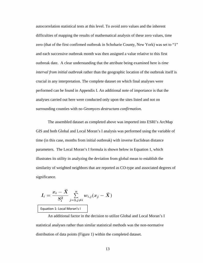
parameters. The Local Moran’s I formula is shown below in Equation 1, which

illustrates its utility in analyzing the deviation from global mean to establish the

similarity of weighted neighbors that are reported as CO-type and associated degrees of

significance.

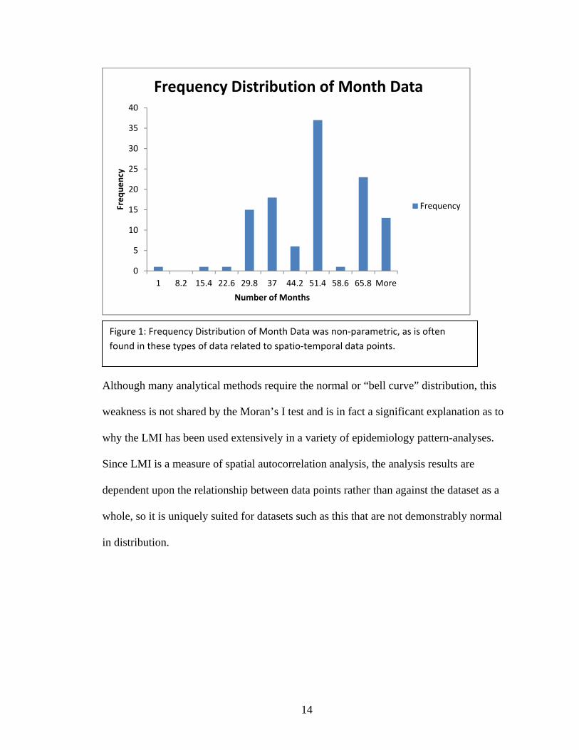
An additional factor in the decision to utilize Global and Local Moran’s I

statistical analyses rather than similar statistical methods was the non-normative

distribution of data points (Figure 1) within the completed dataset.

Equation 1: Local Moran’s I  

14

Although many analytical methods require the normal or “bell curve” distribution, this

weakness is not shared by the Moran’s I test and is in fact a significant explanation as to

why the LMI has been used extensively in a variety of epidemiology pattern-analyses.

Since LMI is a measure of spatial autocorrelation analysis, the analysis results are

dependent upon the relationship between data points rather than against the dataset as a

whole, so it is uniquely suited for datasets such as this that are not demonstrably normal

in distribution.

0

5

10

15

20

25

30

35

40

1 8.2 15.4 22.6 29.8 37 44.2 51.4 58.6 65.8 More

Frequency

Number of Months

Frequency Distribution of Month Data

Frequency

Figure 1: Frequency Distribution of Month Data was non‐parametric, as is often 

found in these types of data related to spatio‐temporal data points. 

15

Results

One of the greatest advantages of graphically displaying the results of the

Moran’s I analyses conducted over the course of this study is that the underlying patterns

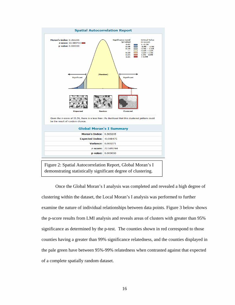
make themselves readily apparent. Results from the Global Moran’s I analysis

demonstrate conclusively that there is indeed an overall clustered pattern upon

examination of the entire dataset as shown below in Figure 2. The large z-score and

extremely small p-value meaningfully show the clustered pattern to have a less than

0.01% chance of being due to random occurrence and strongly indicate that the real

world phenomenon being examined does indeed have a spatiotemporally significant

correlation. Put simply, the overall pattern of infection exhibits a significant grouping of

similar values due primarily to the large number of sites found early on in the epidemic

and this clustered effect is due to the occurrence of Geomyces destructans infection itself

rather than random chance.

16

Once the Global Moran’s I analysis was completed and revealed a high degree of

clustering within the dataset, the Local Moran’s I analysis was performed to further

examine the nature of individual relationships between data points. Figure 3 below shows

the p-score results from LMI analysis and reveals areas of clusters with greater than 95%

significance as determined by the p-test. The counties shown in red correspond to those

counties having a greater than 99% significance relatedness, and the counties displayed in

the pale green have between 95%-99% relatedness when contrasted against that expected

of a complete spatially random dataset.

Figure 2: Spatial Autocorrelation Report, Global Moran’s I demonstrating statistically significant degree of clustering.

17

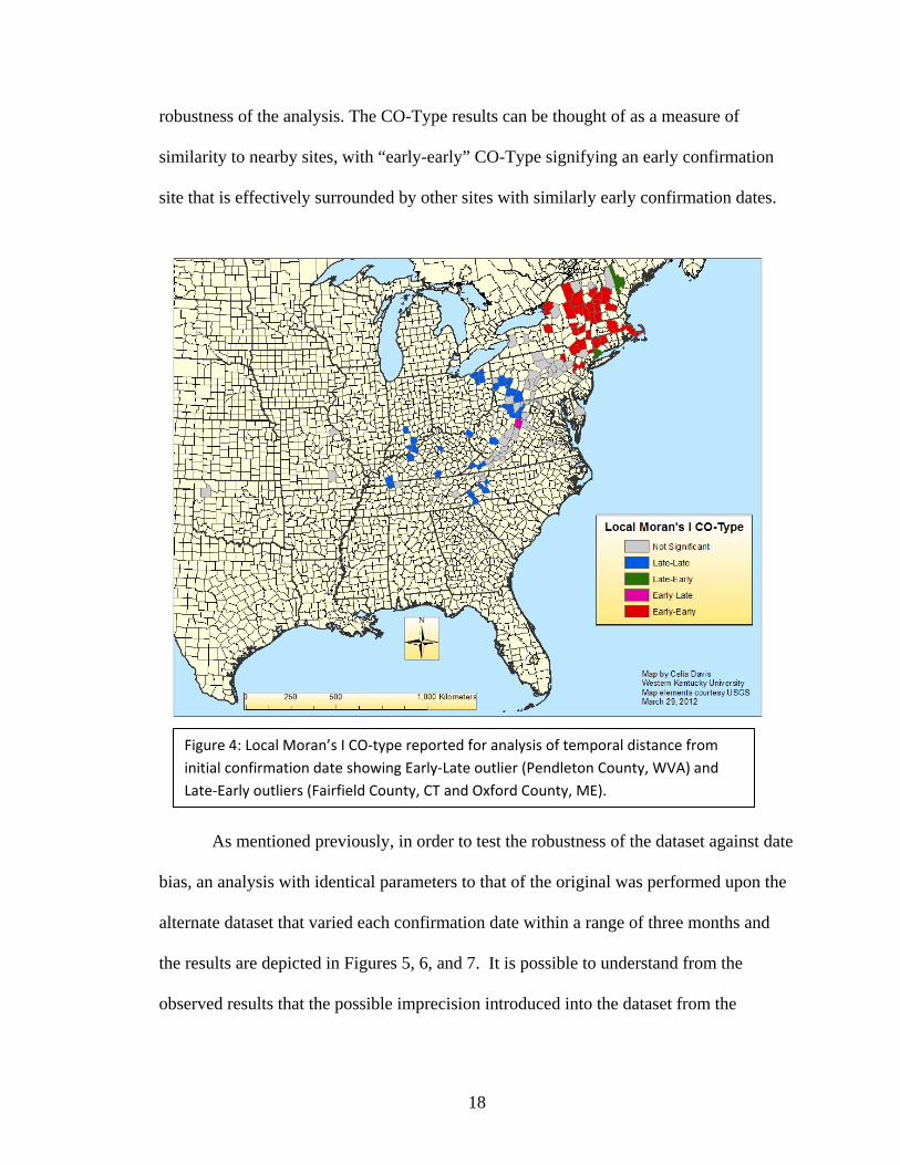
Notably, the areas of significance depicted in Figure 4 correspond to those areas

shown to be clustered under the CO-type analysis reported from LMI conducted on the

temporal assignments of WNS associated fungus confirmation, with those counties with

“early-early” and “late-late” designations having >99% significance (Figure 4). In the

context of this analysis, “early-early” is defined as a data point having low number of

months after initial infection that is surrounded by neighbors of similar values and “late-

late” is defined conversely. The presence of mixed relationships, “late-early” and “early-

late” as shown in dark green and magenta, respectively, is significant based on the

Figure 3: Local Moran’s I p‐score demonstrating areas of significant clustering. 

18

robustness of the analysis. The CO-Type results can be thought of as a measure of

similarity to nearby sites, with “early-early” CO-Type signifying an early confirmation

site that is effectively surrounded by other sites with similarly early confirmation dates.

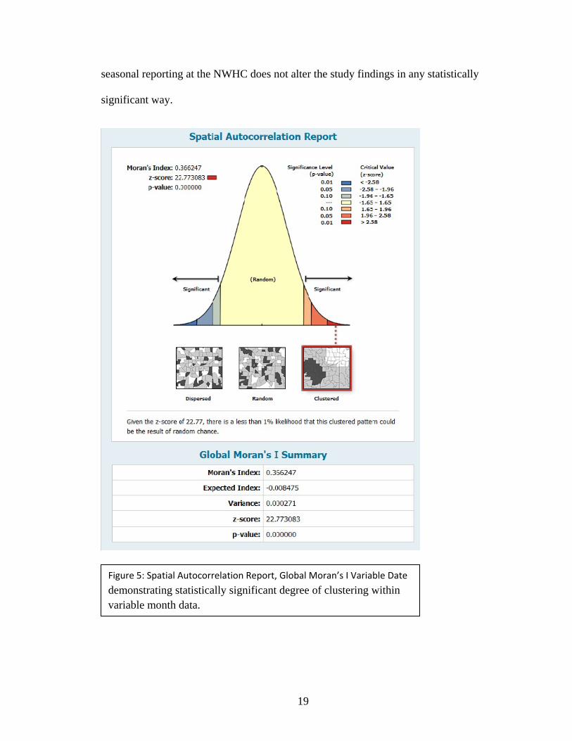
As mentioned previously, in order to test the robustness of the dataset against date

bias, an analysis with identical parameters to that of the original was performed upon the

alternate dataset that varied each confirmation date within a range of three months and

the results are depicted in Figures 5, 6, and 7. It is possible to understand from the

observed results that the possible imprecision introduced into the dataset from the

Figure 4: Local Moran’s I CO‐type reported for analysis of temporal distance from 

initial confirmation date showing Early‐Late outlier (Pendleton County, WVA) and 

Late‐Early outliers (Fairfield County, CT and Oxford County, ME). 

19

seasonal reporting at the NWHC does not alter the study findings in any statistically

significant way.

Figure 5: Spatial Autocorrelation Report, Global Moran’s I Variable Date 

demonstrating statistically significant degree of clustering within variable month data. 

20

Figure 6: Local Moran’s I CO‐type, Variable Date reported for analysis of temporal 

distance from initial confirmation date showing Early‐Late outlier (Pendleton 

County, WVA) and Late‐Early outliers (Fairfield County, CT and Oxford County, ME). 

21

Figure 7: Local Moran’s I p‐scores, Variable Date demonstrating areas of significant 

clustering. 

22

Discussion

Once the labor intensive process of assembling the necessary data into a format

conducive to analysis within the ArcGIS software platform was completed, it became

clear that Moran’s I global and local analysis yielded the most useful information in

determining whether a pattern exists within the data itself (Global Moran’s I, Figures 2

and 5) and, if such a pattern was present, what characterized the nature of that pattern

(Local Moran’s I, Figures 3, 4, 6, and 7). Although a statistically significant clustered

pattern of WNS outbreak sites and dates is present, this is not unexpected due to the

nature of typical disease outbreak and hotspot tendencies as illustrated by the West Nile

virus, meningitis, and Dengue fever outbreaks discussed previously. Of more particular

interest and relevance to the matter at hand is the precise nature of the pattern within the

larger, global clustered pattern, and it is this question that the Local Moran’s I (LMI)

analysis is best suited to answer.

The most unique ability of Moran’s I analysis in this context is the determination

of the presence of so-called “outlier values,” which would indicate a jump-gap

transmission pattern despite the limitations of currently available data (the lack of cave

specific latitude and longitude coordinates and thus “point” data). The aforementioned

limitations of the dataset that make analysis by other methods inappropriate in this

instance are not shared by LMI analysis and this makes it particularly useful in coming to

an understanding of whether the Geomyces destructans fungus believed to be responsible

for WNS follows the roughly linear spread pattern that would be expected from a bat-to-

bat transmission mechanism (single vector with multiple reservoirs) like that shown by

mosquito transmission of West Nile Virus (Sugumaran et al., 2009) or is instead being

23

spread by human transmission from caver gear or clothing from site to site, which would

be reflected by the presence of outliers within the dataset similar to those seen within the

spread of meningitis as previously discussed (Paireau et al., 2012).

Considerable debate has ensued surrounding the nature of WNS dispersal, and

because outliers within Local Moran’s I analysis results occur when an individual data

point is judged to be significantly different in value than its surrounding neighbor

locations, the existence of numerous outliers could be interpreted as evidence of the

“jump dispersal” pattern that might implicate human transmission by visitation to

multiple caves after being in an infected cave as a culprit in the spread of the disease.

Conversely, since only three CO-type outliers were found while performing the LMI

analysis on the WNS mortality confirmation date dataset (Figure 4), the results of this

study suggest that the dominant spread of WNS can be more likely attributed to direct

contact transmission between affected individuals within the bat populations themselves

rather than a human vector model of transmission. Because annual migration of the most

severely affected bat species is limited to distances of 520 km or less for Myotis sodalis

(Kurta and Murray 2002) and 48.5 km for Myotis lucifugus (Butchkoski 2010), the

maximum annual transmission distance of Geomyces destructans by a bat carrier would

be within that range based on the current transmission data. In contrast, human carriers

could potentially travel well in excess of the above stated migration limits and thus

“seed” a location with the fungus at much greater distances. If such a long-distance

seeding were to occur by human carriers as a matter of routine transmission, the resulting

White-Nose Syndrome mortality confirmation site would be revealed as an outlier with a

24

value earlier than that of surrounding confirmed sites (or an “early-late” outlier within the

LMI analysis as performed in this study).

The two “late-early” outliers found in Fairfield County, Connecticut and Oxford

County, Maine (Figure 6) represent counties in which the Geomyces destructans fungus

was detected at a statistically significant later date than those counties nearest the sites,

and suggests that these counties may possess some topographical or ecological variation

which prevented the spread of WNS into bat populations there at earlier dates.

Alternatively, the surveying interval due to cave or mine access issues, or lack of

surveying resources or personnel, could account for the difference in detection date; the

fungus may have been present prior to reporting date but due to a delay in survey, was

not discovered until later in the epidemic. Since the emphasis on most disease

transmission research is the front edge of an epidemic, these “late-early” outliers are of

potential interest in exploring what factors may have played a role in the transmission

delay, however do little to explicate the underlying dispersal mechanism.

Of more concern and relevance to understanding the dispersal pattern of

Geomyces destructans is the Pendleton County, West Virginia (WV) site (Figure 6) that

is shown to be an “early-late” outlier by Local Moran’s I analysis. The presence of such

an outlier could be interpreted as support for a “human as vector” model of disease

transmission, and in fact, if analysis had revealed a pattern of such outliers, such a

conclusion could be meaningfully drawn. However, closer examination of the dataset,

particularly those counties surrounding Pendleton County, reveals that counties south of

the site (Giles confirmed 2/2009, Bland confirmed 5/2009) showed earlier infection. The

seven counties surrounding Pendleton County show considerable variation in reported

25

dates (Figure 6- Pocohantas WV on 3/2010, Highland VA on 4/10, Rockingham VA on

8/2009, Tucker WV on 2/2011, Grant WV on 4/2011, Hardy WV on 3/2010, and Bath

VA on 2/2009), and this constellation of occurrence dates suggests that the outlier status

of Pendleton County, WV is perhaps a reflection of reporting artifacts and the much later

reporting of Tucker and Grant counties in West Virginia is sufficiently later to alter the

statistical analysis reporting of CO-type status even when weighed against the earlier

dates of surrounding counties. Given the inherent financial, time, and access resource

constraints placed on survey efforts in the mountains of West Virginia, it is possible that

earlier appearances of the fungus were unrecorded.

When the analysis was performed again using a dataset that had been artificially

altered to reflect a degree of three month variability in either the forward or backward

temporal direction, the results did not differ in any statistically meaningful way from the

original dataset, and again revealed a pattern with two clusters (early-early and late-late)

along with the presence of outlier values for Pendleton County, WV, Fairfield County,

CT, and Oxford County, Maine (Figures 5, 6, and 7). Performing the Moran’s I analyses

on a dataset in which the data points had been randomly altered by three months

addressed a potential vulnerability of the analysis because of the possible variation in

confirmation reporting dates due to the inherent difficulty in obtaining primary data;

timing of cave surveys, difficulty in accessing hibernaculum sites, and seasonal

limitations all have the effect of introducing a possible “timing artifact” bias into the

results. It also addresses the possible issue of sensitivity of the analysis to be able to

detect outliers within a larger reporting error. The variable month dataset and analysis

results effectively demonstrate that the nature of the pattern found in this study is a

26

reflection of the actual phenomenon being examined rather than a side-effect of the

unavoidable data collection limitations. Had there been an alteration of outlier values in

the CO-type reporting by such an alteration of the dataset, the veracity of such a

statistical analysis could rightly be questioned. However, in this case, the affirmation by a

high degree of similarity of reported values further emphasizes the robust nature of the

analysis itself.

Ultimately, the results of this study, primarily the lack of multiple “early-late”

outlier values as revealed by Local Moran’s I CO-type reporting and associated

significance values (Figures 3 and 4), suggest that the dominant transmission pattern of

White-Nose Syndrome in the United States is typical of that found in diseases

characterized by direct transmission between individuals of affected bat species rather

than that of a separate vector. One would expect that if humans were acting as a vector

for Geomyces destructans, the dispersal pattern would resemble that of meningitis as

discussed above and outlier values representing “jumps” in the dispersal would be

present. This finding is contrary to much of what has been supposed about the dispersal

of WNS and further emphasizes just how critical the creation of, and continued efforts to

maintain, a comprehensive dataset of outbreak data is to appropriately address the issue at

hand and arrive at policies that more effectively mitigate White-Nose Syndrome. As any

research is limited to the quality of data upon which the analyses are performed, the

discrepancy around the Pendleton, WV confirmation dates should serve as a strong

reminder of how critically important the practice of standardized, rigorous data collection

is to our understanding of the timing and occurrence of natural phenomena like infectious

disease dispersal patterns. Additionally, because such robust data collection is made even

27

more difficult with diminished resources, it should serve as a call for increased attention

to communication and management at both the state and federal levels in order to more

promptly develop monitoring and surveying plans, and mobilize “ground troops” for

future outbreaks.

A more complete understanding of the dispersal patterns of White-Nose

Syndrome, as revealed by careful statistical evaluation of the relationships between each

confirmed site within the compiled dataset, is absolutely critical to the development of a

scientifically valid, well-reasoned approach to addressing and possibly mitigating the

devastating effects of WNS. Previously, such large-scale studies have not been

conducted due in part to the lack of a comprehensive dataset and, now that the stated

research goal of establishing such a dataset and determining its usefulness has been

accomplished here, more scientifically rigorous evaluations of the dispersal patterns

found within the epidemic can be built upon the results of this study. Of particular

interest for future mitigation efforts could be the development of a dataset that compares

Geomyces destructans infection dates against WNS associated mortality dates. Such a

dataset would allow for the detailed examination of transmission and mortality

expression rates and could potentially reveal crucial information about factors which

influence disease development, however that data is not yet available and will take

considerable cooperation and effort to develop into a meaningful investigative tool.

In addition to the chronological and temporal analysis of the disease spread itself,

perhaps one of the most powerful aspects of applying ArcMap’s graphical capabilities to

an examination of this disease spread pattern is that alternate variables, such as

topography, prevailing wind patterns, and migration paths, can be incorporated into

28

further analyses. Although it is impossible to predict at this stage which of these

variables, if any, will prove to be significant upon further examination, the fact that the

Geomyces destructans fungus is cold-loving and therefore potentially affected by factors

such as annual temperature and geomorphology of the hibernaculum themselves strongly

suggests that a correlation with these annual temperatures and dominant wind patterns

should present itself when used as a co-variable against the spread pattern and resulting

mortality. As of completion of this study, wide-ranging efforts are underway to establish

robust baseline population numbers for affected bat species. These census efforts

coupled with more sophisticated mortality counts could potentially allow further research

into how the climatic and ecological factors mentioned above play a role in individual

and population survivability.

Most current mitigation techniques have involved closing caves or mines, or

limiting access by humans, along with evolving decontamination procedures (USFWS,

2012a,b). A better understanding of the fungus itself and its survivability in various

environments from recent research also introduced continued discussion about how best

to address WNS issues (Blehert 2011). However, many of the current efforts to curtail the

spread of Geomyces destructans have been hampered by an incomplete understanding of

the underlying patterns of dispersal, combined with the lack of a standardized method of

disease discovery and reporting. Additionally, the policies in place at the federal and state

government level regarding well-intentioned cave and mine closures may have had the

unintentional effect of diminishing beneficial input from potential allies within the

outside community. Given that eventual modeling efforts will be largely dependent on

the robustness of site data (both spatial and temporal) and the large role played by non-

29

governmental visitors in establishing outbreak sites early in the disease, the decision to

close all caves and mines on public land may have the end result of decreasing our ability

to reasonably predict where and when future outbreaks will occur.

In order to effectively collect and compile a current dataset of ongoing outbreak

sites, it will be necessary to establish a clearinghouse for suspected WNS sites at the

federal level with a correspondingly rigorous protocol to determine data accuracy and

what criteria by which to include new sites. For the purposes of this study, WNS

associated mortality was not a prerequisite for inclusion in the dataset; however, the

nature of the causative fungus and manifestation of WNS mortality itself is as of yet

incompletely understood with some species exhibiting symptoms of WNS with no

resulting mortality (USFWS, 2012b). As survey and census efforts intensify, more

comprehensive data on sites infected with Geomyces destructans prior to mortality events

may well lead to important discoveries regarding species susceptibility and survivability.

Perhaps of most urgent import to wildlife managers and conservation efforts is the

ability to more effectively predict the areas which Geomyces destructans is most likely to

infect and when it will affect those areas. The novel application of Moran’s I used in this

research suggests that, not only would it be possible to create predictive geospatial

models, but that transmission time itself can be used as a variable when constructing

these predictive models. This study provides an example or the robustness of these

techniques and their ability to play a crucial role in management activities associated with

WNS and future outbreaks, while also illustrating the limitations of the analysis given the

myriad data collection and reporting techniques used to date. This has significant

30

implications not just for the disease being examined within the context of this study, but

for the broader field of wildlife epidemiology as a whole.

31

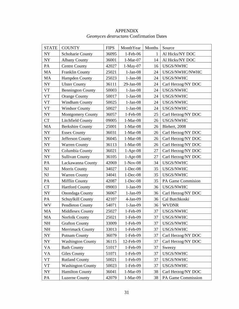
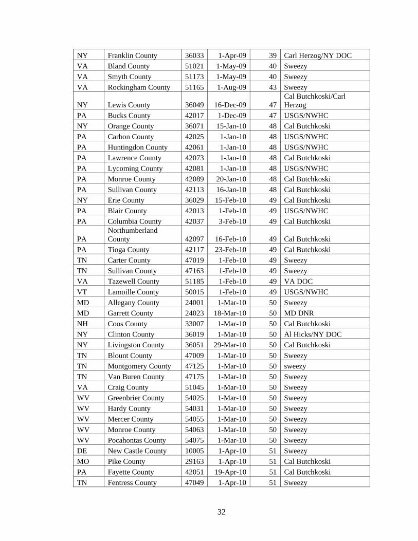
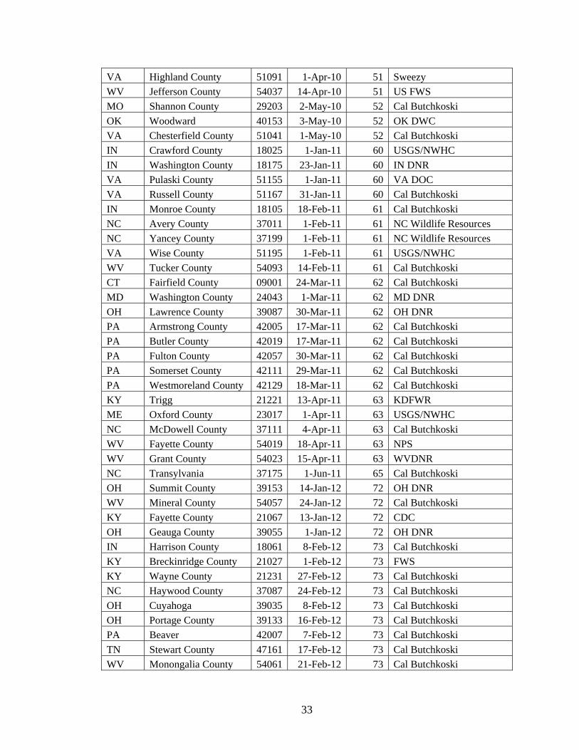
APPENDIX Geomyces destructans Confirmation Dates

STATE COUNTY FIPS MonthYear Months Source

NY Schoharie County 36095 1-Feb-06 1 Al Hicks/NY DOC

NY Albany County 36001 1-Mar-07 14 Al Hicks/NY DOC

PA Centre County 42027 1-May-07 16 USGS/NWHC

MA Franklin County 25021 1-Jan-08 24 USGS/NWHC/NWHC

MA Hampden County 25023 1-Jan-08 24 USGS/NWHC

NY Ulster County 36111 29-Jan-08 24 Carl Herzog/NY DOC

VT Bennington County 50003 1-Jan-08 24 USGS/NWHC

VT Orange County 50017 1-Jan-08 24 USGS/NWHC

VT Windham County 50025 1-Jan-08 24 USGS/NWHC

VT Windsor County 50027 1-Jan-08 24 USGS/NWHC

NY Montgomery County 36057 1-Feb-08 25 Carl Herzog/NY DOC

CT Litchfield County 09005 1-Mar-08 26 USGS/NWHC

MA Berkshire County 25001 1-Mar-08 26 Blehert, 2008

NY Essex County 36031 1-Mar-08 26 Carl Herzog/NY DOC

NY Jefferson County 36045 1-Mar-08 26 Carl Herzog/NY DOC

NY Warren County 36113 1-Mar-08 26 Carl Herzog/NY DOC

NY Columbia County 36021 1-Apr-08 27 Carl Herzog/NY DOC

NY Sullivan County 36105 1-Apr-08 27 Carl Herzog/NY DOC

PA Lackawanna County 42069 1-Nov-08 34 USGS/NWHC

NJ Morris County 34027 1-Dec-08 35 USGS/NWHC

NJ Warren County 34041 1-Dec-08 35 USGS/NWHC

PA Mifflin County 42087 1-Dec-08 35 PA Game Commision

CT Hartford County 09003 1-Jan-09 36 USGS/NWHC

NY Onondaga County 36067 1-Jan-09 36 Carl Herzog/NY DOC

PA Schuylkill County 42107 4-Jan-09 36 Cal Butchkoski

WV Pendleton County 54071 1-Jan-09 36 WVDNR

MA Middlesex County 25027 1-Feb-09 37 USGS/NWHC

MA Norfolk County 25021 1-Feb-09 37 USGS/NWHC

NH Grafton County 33009 1-Feb-09 37 USGS/NWHC

NH Merrimack County 33013 1-Feb-09 37 USGS/NWHC

NY Putnam County 36079 1-Feb-09 37 Carl Herzog/NY DOC

NY Washington County 36115 12-Feb-09 37 Carl Herzog/NY DOC

VA Bath County 51017 1-Feb-09 37 Sweezy

VA Giles County 51071 1-Feb-09 37 USGS/NWHC

VT Rutland County 50021 1-Feb-09 37 USGS/NWHC

VT Washington County 50023 1-Feb-09 37 USGS/NWHC

NY Hamilton County 36041 1-Mar-09 38 Carl Herzog/NY DOC

PA Luzerne County 42079 1-Mar-09 38 PA Game Commission

32

NY Franklin County 36033 1-Apr-09 39 Carl Herzog/NY DOC

VA Bland County 51021 1-May-09 40 Sweezy

VA Smyth County 51173 1-May-09 40 Sweezy

VA Rockingham County 51165 1-Aug-09 43 Sweezy

NY Lewis County 36049 16-Dec-09 47Cal Butchkoski/Carl Herzog

PA Bucks County 42017 1-Dec-09 47 USGS/NWHC

NY Orange County 36071 15-Jan-10 48 Cal Butchkoski

PA Carbon County 42025 1-Jan-10 48 USGS/NWHC

PA Huntingdon County 42061 1-Jan-10 48 USGS/NWHC

PA Lawrence County 42073 1-Jan-10 48 Cal Butchkoski

PA Lycoming County 42081 1-Jan-10 48 USGS/NWHC

PA Monroe County 42089 20-Jan-10 48 Cal Butchkoski

PA Sullivan County 42113 16-Jan-10 48 Cal Butchkoski

NY Erie County 36029 15-Feb-10 49 Cal Butchkoski

PA Blair County 42013 1-Feb-10 49 USGS/NWHC

PA Columbia County 42037 3-Feb-10 49 Cal Butchkoski

PA Northumberland County 42097 16-Feb-10 49 Cal Butchkoski

PA Tioga County 42117 23-Feb-10 49 Cal Butchkoski

TN Carter County 47019 1-Feb-10 49 Sweezy

TN Sullivan County 47163 1-Feb-10 49 Sweezy

VA Tazewell County 51185 1-Feb-10 49 VA DOC

VT Lamoille County 50015 1-Feb-10 49 USGS/NWHC

MD Allegany County 24001 1-Mar-10 50 Sweezy

MD Garrett County 24023 18-Mar-10 50 MD DNR

NH Coos County 33007 1-Mar-10 50 Cal Butchkoski

NY Clinton County 36019 1-Mar-10 50 Al Hicks/NY DOC

NY Livingston County 36051 29-Mar-10 50 Cal Butchkoski

TN Blount County 47009 1-Mar-10 50 Sweezy

TN Montgomery County 47125 1-Mar-10 50 sweezy

TN Van Buren County 47175 1-Mar-10 50 Sweezy

VA Craig County 51045 1-Mar-10 50 Sweezy

WV Greenbrier County 54025 1-Mar-10 50 Sweezy

WV Hardy County 54031 1-Mar-10 50 Sweezy

WV Mercer County 54055 1-Mar-10 50 Sweezy

WV Monroe County 54063 1-Mar-10 50 Sweezy

WV Pocahontas County 54075 1-Mar-10 50 Sweezy

DE New Castle County 10005 1-Apr-10 51 Sweezy

MO Pike County 29163 1-Apr-10 51 Cal Butchkoski

PA Fayette County 42051 19-Apr-10 51 Cal Butchkoski

TN Fentress County 47049 1-Apr-10 51 Sweezy

33

VA Highland County 51091 1-Apr-10 51 Sweezy

WV Jefferson County 54037 14-Apr-10 51 US FWS

MO Shannon County 29203 2-May-10 52 Cal Butchkoski

OK Woodward 40153 3-May-10 52 OK DWC

VA Chesterfield County 51041 1-May-10 52 Cal Butchkoski

IN Crawford County 18025 1-Jan-11 60 USGS/NWHC

IN Washington County 18175 23-Jan-11 60 IN DNR

VA Pulaski County 51155 1-Jan-11 60 VA DOC

VA Russell County 51167 31-Jan-11 60 Cal Butchkoski

IN Monroe County 18105 18-Feb-11 61 Cal Butchkoski

NC Avery County 37011 1-Feb-11 61 NC Wildlife Resources

NC Yancey County 37199 1-Feb-11 61 NC Wildlife Resources

VA Wise County 51195 1-Feb-11 61 USGS/NWHC

WV Tucker County 54093 14-Feb-11 61 Cal Butchkoski

CT Fairfield County 09001 24-Mar-11 62 Cal Butchkoski

MD Washington County 24043 1-Mar-11 62 MD DNR

OH Lawrence County 39087 30-Mar-11 62 OH DNR

PA Armstrong County 42005 17-Mar-11 62 Cal Butchkoski

PA Butler County 42019 17-Mar-11 62 Cal Butchkoski

PA Fulton County 42057 30-Mar-11 62 Cal Butchkoski

PA Somerset County 42111 29-Mar-11 62 Cal Butchkoski

PA Westmoreland County 42129 18-Mar-11 62 Cal Butchkoski

KY Trigg 21221 13-Apr-11 63 KDFWR

ME Oxford County 23017 1-Apr-11 63 USGS/NWHC

NC McDowell County 37111 4-Apr-11 63 Cal Butchkoski

WV Fayette County 54019 18-Apr-11 63 NPS

WV Grant County 54023 15-Apr-11 63 WVDNR

NC Transylvania 37175 1-Jun-11 65 Cal Butchkoski

OH Summit County 39153 14-Jan-12 72 OH DNR

WV Mineral County 54057 24-Jan-12 72 Cal Butchkoski

KY Fayette County 21067 13-Jan-12 72 CDC

OH Geauga County 39055 1-Jan-12 72 OH DNR

IN Harrison County 18061 8-Feb-12 73 Cal Butchkoski

KY Breckinridge County 21027 1-Feb-12 73 FWS

KY Wayne County 21231 27-Feb-12 73 Cal Butchkoski

NC Haywood County 37087 24-Feb-12 73 Cal Butchkoski

OH Cuyahoga 39035 8-Feb-12 73 Cal Butchkoski

OH Portage County 39133 16-Feb-12 73 Cal Butchkoski

PA Beaver 42007 7-Feb-12 73 Cal Butchkoski

TN Stewart County 47161 17-Feb-12 73 Cal Butchkoski

WV Monongalia County 54061 21-Feb-12 73 Cal Butchkoski

34

WV Preston County 54077 27-Feb-12 73 Cal Butchkoski

35

REFERENCES

Anselin L. 1995. Local Indicators of Spatial Association—LISA. Geographical Analysis. 27(2):93-115. Blehert D.S., A.C. Hicks, M. Behr, C.U. Meteyer, B. Berlowski-Zier, E.L. Buckles, J.T.H. Coleman, S.R. Darling, A. Gargas, R. Niver, J.C. Okoniewski, R.J. Rudd, and W.B. Stone. 2009. Bat White-Nose syndrome: an emerging fungal pathogen? Science. 323(5911):227 Boyles J.G., Cryan P.M., McCraken G.F., and Kunz T.H. 2011. Economic Importance of Bats in Agriculture. Science. 332:41-42. Butchkoski C. 2010. Indiana Bat (Myotis sodalis) Summer Roost Investigations. Pennsylvania Game Commission Bureau Of Wildlife Management Project Annual Job Report. February 25, 2010. Carnes A. and Ogneva-Himmelberger Y. 2011. Temporal Variations in the Distribution of West Nile Virus Within the United States; 2000-2008. Applied Spatial Analysis and Policy. DOI: 10.1007/s12061-011-9067-7 Clark D.R. Jr., C.M. Bunck, and E. Cromartie. 1983. Year and age effects on residues of Dieldrin and Heptachlor in dead gray bats, Franklin County, Missouri-1976, 1977, and 1978. Environmental Toxicology and Chemistry. 2:387-393 Cleveland C.J., M. Betke, P. Federico, J.D. Frank, T.G. Hallam, J. Horn, J.D. Lopez Jr., G.F. McCracken, R.A. Medillin, A. Moreno-Valdez, C.G. Sansone, J.K. Westbrook, and T.H. Kunz. 2006. Economic value of the pest control service provided by Brazilian free-tailed bat in south-central Texas. Frontiers in Ecology and Environment 4:238–243. Cryan P., Meteyer C., Boyles J., and Blehert D. 2010. Wing pathology of White-Nose syndrome in bats suggests life-threatening disruption of physiology. BMC Biology.8(1):135. FAO. (Food and Agriculture Organization of the United Nations). 2009. The State of Food Insecurity in the World: Economic crises – impacts and lessons learned. Accessed 10/20/10. http://www.fao.org/docrep/012/i0876e/i0876e00.htm  

Frick W.F., Pollock J.F., Hicks A.C., Langwig K.E., Reynolds D.S., Turner G.G., Butchkoski C.M., and Kunz T, H. 2010. An Emerging Disease Causes Regional Population Collapse of a Common North American Bat Species. Science. 329:679-682. Gargas A., M.T. Trest, M. Christensen, T.J. Volk, and D.S. Blehert. 2009. Geomyces destructans sp. Nov. associated with bat White-Nose syndrome. Mycotaxon. 108:147-154

36

Geluso K.N., J.S. Altenbach and D.E. Wilson. 1976. Bat mortality: pesticide poisoning and migratory stress. Science. 194:184–186 Johnson, R. 2007. Honey Bee Colony Collapse Disorder. Congressional Research Service, The Library of Congress. Washington, D.C. Report date June 20, 2007. Jones G., D.S Jacobs, T.H. Kunz, M.R. Willig, and P.A. Racey. 2009. Carpe noctem: The importance of bats as bioindicators. Endangered Species Research. 8:93-115 Kalka Margareta B., Smith A.R, and Kalko, E.K.V. 2008. Bats limit arthropods and herbivory in a tropical forest. Science. 320(5872):71 Kurta A., and Murray S.W. 2002. Philopatry and migration of banded Indiana bats (Myotis sodalis) and effects of using transmitters. Journal of Mammalogy.83:585-589. Lorch J.M., Meteyer C.U., Behr M.J., Boyles J.G., Cryan P.M., Hicks A.C., Ballmann A.E., Coleman J.T.H., Redell D.N., Reeder D.M, and Blehert D.S. 2011. Experimental infection of bats with Geomyces destructans causes white-nose syndrome. Nature. October 26, 2011. doi:10.1038/nature10590.

McKee Jr., K.T., Shields, T.M., Jenkins, P.R., Zenilman, J.M., and Glass, G.E. 2000. “Application of a Geographic Information System to the Tracking and Control of an Outbreak of Shigellosis.” Clinical Infectious Diseases. 31(3):728-733. Meteyer, C.U., Loeffler, I.K., Fallon, J.F., Converse, K.A., Green, E., Helgen, J.C., Kersten, S., Levey, R., Eaton-Poole, L., Burkhart, J,G,. 2000. Hind Limb Malformations in Free-Living Northern Leopard Frogs (Rana pipiens) From Maine, Minnesota, and Vermont Suggest Multiple Etiologies. Teratology. 62:151-171. Morrison, A.C., Getis, A., Santiago, M., Rigua-Perez, J.G., and Reiter, P. 1998. “Exploratory space-time analysis of reported dengue cases during an outbreak in Florida, Puerto Rico, 1991-1992.” American Journal of Tropical Medicine and Hygiene. 58(3):287-298 Nakhapakorna,K. and Jirakajohnkoolb, S. 2006. “Temporal and Spatial Autocorrelation Statistics of Dengue Fever.” Dengue Bulletin. Volume 30:177-183. Published by World Health Organization. National Wildlife Health Center. Division of the United States Geological Survey. http://www.nwhc.usgs.gov/publications/quarterly_reports. Accessed 3/2011-5/2011. O’Sullivan D., and Unwin D.J. 2003. Geographic Information Analysis. John Wiley & Sons. Hoboken, New Jersey.

37

Paireau J., Girond F., Collard, J-M., Maïnassara H.B., Jusot J.F. 2012. Analysing Spatio-Temporal Clustering of Meningococcal Meningitis Outbreaks in Niger Reveals Opportunities for Improved Disease Control. PloS Neglected Tropical Diseases. March; 6(3):e1577. Reichard, J.D., and T.H. Kunz. 2009. White-Nose Syndrome inflicts lasting injuries to the wings of little brown myotis (Myotis lucifugus). Acta Chiropterologica. 11:457-464. Sugumaran, R., Larson, S.R., and DeGroote, J.P. 2009. “Spatio-temporal cluster analysis of county-based human West Nile virus incidence in the continental United States.” International Journal of Health Geographics. 8:43. Swezey, C. and Garrity, C. 2010. “Notes On The Geology And Meteorology of Sites Infected With White-Nose Syndrome Before July 2010 in the Southeastern United States”. U.S. Geological Survey. Reston, VA. Turbill, C., and F. Geiser. 2008. Hibernation in tree-roosting bats. Journal of Comparative Physiology. 178B:597–605. United States Fish and Wildlife Service. 2012a. White-Nose Syndrome Decontamination Protocol-Version 03.15.2012. www.fws.gov/WhiteNoseSyndrome/pdf/National _WNS_Decontamination _Protocol_v03.15.2012.pdf. Last accessed 7/3/2012.  

Unites States Fish and Wildlife Service. 2012b. May 12 News Release. www.caves.org/WNS/Gray_bats_2012_NR_Final.pdf. Last accessed 7/5/12. United States Fish and Wildlife Service. 2012c. White-Nose Syndrome Message to Cavers. www.fws.gov/WhiteNoseSyndrome/cavers.html. Last accessed 7/3/12. United States Fish and Wildlife Service. 2012d. U.S. Fish and Wildlife Service Awards Grants to 30 States for White-Nose Syndrome Work. www.batcon.org/pdfs/whitenose/2012%20WNS%20grant. Last accessed 7/26/12. Wibbelt G., A. Kurth, D. Hellmann, M. Weishaar, A. Barlow, M. Veith, J. Prüger, T. Görföl, L. Grosche, F. Bontadina, U. Zöphel, H.P. Seidl, P.M. Cryan, and D.S. Blehert. 2010. White-Nose Syndrome Fungus (Geomyces destrucatns) in Bats, Europe. Emerging Infectious Diseases. 16(8):1237-1242.  

Wickramasinghe L.P., S. Harris, G. Jones, and N.V. Jennings. 2004. Abundance and species richness of nocturnal insects on organic and conventional farms: effects of agricultural intensification on bat foraging. Conservation Biology. 18:1283–1292. Willis C.K.R., Menzies A.K., Boyles J.G., and Wojciechowski M.S. 2011. Evaporative Water Loss Is a Plausible Explanation for Mortality of Bats from White-Nose Syndrome. Integrative and Comparative Biology. 51:6.

38

Yeshiwondim, A.K., Gopal, S., Hailemariam, A.T., Dengela, D.O., and Patel, H.P. 2009. “Spatial analysis of malaria incidence at the village level in areas with unstable transmission in Ethiopia.” International Journal of Health Geographics. 8:5.Ope