an evaluation of the federal reserve bank of boston's study of … · i an evaluation of the...

i

An Evaluation of the Federal Reserve Bank of Boston's Study of Racial Discrimination in Mortgage Lending

Dennis Glennon and Mitchell Stengel

Office of the Comptroller of the CurrencyEconomic & Policy Analysis

Working Paper 94 -2April 1994

Abstract: In 1992, the Federal Reserve Bank of Boston (Boston Fed) released a now well-knownstudy of mortgage lending practices in the Boston Metropolitan Statistical Area (MSA). Usingan econometric model to examine extensive mortgage loan data collected from 131 financialinstitutions in the Boston MSA, the authors of the Boston Fed study tried and failed to findexplanations other than racial discrimination for the significant disparities observed in the rejectionrates for white and minority loan applicants.

The Boston Fed study attracted considerable attention from Congress, the banking industry, thecivil rights community, bank regulators, and the news media. But three follow-up studies haveraised a variety of problems with the Boston Fed study relating to data and methodology.

In this paper, we discuss and evaluate the problems cited by critics of the Boston Fed study. Wefocus our attention on three broad areas of concern: model specification; data errors; anddifferences in characteristics of the groups being compared.

Our principal findings can be summarized as follows:(i) Several alternative model specifications perform better than the Boston Fed model in terms

of various econometric performance measures; however, the race of the applicantcontinues to have a large and highly significant effect on the outcome of the lendingapplication process.

(ii) The results of the Boston Fed model are affected only slightly when some of the moreobvious and easily correctable data errors are corrected.

(iii) Allowing for different coefficients for whites and minorities, our analysis supports theBoston Fed' s conclusion that approximately half the difference in denial rates can beattributed to differences in the financial characteristics of the borrowers and theneighborhood characteristics of the property; the remaining half can be attributed todifferences in treatment by race.

iii

We conclude with a qualified confirmation of the results of the Boston Fed study. However, webelieve there are still several important specification issues that cannot be investigated and severaldata problems that cannot be corrected using the data provided by the Boston Fed. Additionalresearch at both the MSA and the individual bank levels is warranted.

_____________________________________________________________________________

The opinions expressed are those of the authors and do not necessarily represent those of the Office of the Comptroller

of the Currency. The authors would like to thank Jeffrey Brown, Michael Carhill, Julia Lane, Kevin Jaques, Daniel

Nolle, and Mark Winer for helpful comments. Any errors are the responsibility of the authors.

Please address questions of substance to the authors at the Economic & Policy Analysis Department, Office of the

Comptroller of the Currency, 250 E Street, Washington, D.C. , 20219, (202) 874-5240.

1

I. Introduction

The Federal Reserve Bank of Boston' s study of mortgage lending practices in the Boston MSA(Munnell et al. 1992) has redefined the debate over the existence of racial discrimination inmortgage lending. Using a much more extensive data set than any previous study, the Boston Fedanalyzed differences in denial rates across races after controlling for wealth, credit andemployment histories. The authors conclude that ". . . even after controlling for financial,employment, and neighborhood characteristics, Black and Hispanic mortgage applicants in theBoston metropolitan area are roughly 60 percent more likely to be turned down than whites"(Munnell et al. 1992, p. 2). They attribute the difference to discrimination on the part of thelending institutions. For many, the Boston Fed study seemed to answer ) once and for all ) thequestion of whether racial discrimination exists in mortgage lending. Moreover, the results of thestudy were a major impetus in the renewed and intensified efforts of the federal government todetect, punish, and eradicate such discrimination.

In recent months, however, three follow-up studies have identified several data andmethodological problems that appear to call into question the Boston Fed' s central finding ofsubstantial discrimination against minorities (Horne 1994; Liebowitz 1993; Zandi 1993). In thispaper, we discuss several of the issues raised by the follow-up studies. We focus our attentionon three broad areas of concern, model misspecification, data errors, and differences in initialendowments. We find many of the criticisms of the Boston Fed' s method of specifying andassessing the accuracy of their model to be legitimate. There are reasonable arguments supportingalternative model specifications that may better capture the underwriter' s decision-making process.Moreover, we find that there are unquestionably numerous data entry and data reporting errorsin the information supplied by the institutions that participated in the study. Nevertheless, usingdata provided by the Boston Fed, we test several alternative specifications of the model and findtheir results ) including the magnitude and significance of the race variable ) to be quite robustwith regard both to alternative specifications and to the correction of the more obvious and easilycorrectable data errors. Moreover, we find that approximately half of the difference in observeddenial rates can be attributed to differences in the initial endowments (i.e. , the basic characteristicsof the applicants or the properties) associated with individual racial groups, and that the remainingdifference in the denial rates represents a discriminatory differential of roughly the samemagnitude as that found by the original study.

The follow-up studies also raise several other methodological and sample design problems that,if valid, could substantially alter the Boston Fed' s conclusion. For the most part, however, thoseissues cannot be tested using the Boston Fed data and therefore are speculative at best. We assessthe validity of these criticisms as applied to the Boston Fed study, and where possible, discuss thelikely impact they would have on the results.

The paper is structured as follows. In the next section, we summarize the Boston Fed' smethodology and findings. Section III introduces the issues of goodness-of-fit and separateregression models for whites and minorities. Section IV explores the question of differences in

The initial sample design developed by the Boston Fed identified all 1210 minority (Black and Hispanic)1

applicants in the Boston MSA in 1990 for inclusion; however, for practical reasons, the Boston Fed chose to

survey only institutions that had received at least 25 mortgage applications from borrowers of all races.

Sixty-seven minority applications were lost from the survey for this reason. Information then was requested

from the 1,143 applicants for conventional mortgage loans made to Blacks and Hispanics and from a random

sample of the 3,300 white applicants filed in the Boston MSA in 1990. Bank failures, inability to locate all

requested loan files, and corrections to earlier submissions reduced the final sample size to 3,062 (2,340

white, and 1,013 minority applicants).

By design, the Boston Fed sample included a larger proportion of minorities than whites; the final sample

contained 59.7 percent of all minority applications from the MSA in 1990, and 14.6 percent of the whites.

Disproportionate sampling of this type is quite common and often well-justified in logit regression studies.

It is generally done in order to guarantee that the sample contains adequate numbers of the groups least

represented in the total population, in this case minorities in general and denied minorities in particular.

While a common practice, disproportionate sampling does pose certain technical problems in terms of the

validity of the regression results, and different authors have proposed various corrective techniques. (See

Maddala 1983, pp. 90-91, for discussion.) We applied two such techniques, a weighted regression and an

intercept adjustment, to the Boston Fed model. Neither had any substantial effect on

2

endowments by race. In section V, we discuss several alternative model specifications that webelieve better represent the underwriting procedure employed in the mortgage lending market.In section VI, a summary and discussion of some of the more troubling data errors are presentedand issues of model misspecification and omitted variables are also explored. We conclude withan overall assessment of the validity of the Boston Fed' s findings with regard to the existence ofdiscrimination, and a discussion of future research efforts.

II. The Boston Fed model

The Boston Fed found that Home Mortgage Disclosure Act (HMDA) data consistently show thatnon-Asian minority home mortgage application denial rates are two to three times higher thanthose for whites. This led Munnell et al. to argue:

[t]his pattern has triggered a resurgence of the debate on whether discrimination exists inhome mortgage lending. Some people believe that the disparities in denial rates areevidence of discrimination on the part of banks and other lending institutions. Others,including lenders, argue that such conclusions are unwarranted, because the HMDA datado not include information on credit histories, loan-to-value ratios, and other factorsconsidered in making mortgage decisions. These missing pieces of information, theyargue, explain the high denial rates for minorities (Munnell et al. 1992, p. 1).

The Boston Fed sought to resolve this controversy, at least in the case of a single MSA, byconducting a follow-up study. With the voluntary participation of the lending institutions, theycollected information on the creditworthiness of applicants from all HMDA-reporting institutionsin the Boston MSA that received at least total 25 mortgage applications in 1990. A final sampleof 3,062 files (2,340 white and 1,013 Hispanic and Black) was chosen from 18,838 total loanapplications. An expanded HMDA data form was then sent to each institution, requesting1

the signs, magnitudes, or significance levels of the estimated coefficients, including the race variable; nor was

there any appreciable impact on the various measures of goodness-of-fit.

In the estimation procedure, 2

g(x) = âx

where x = independent variables, and

â = estimated parameters.

Since the dependent variable can take on only one of two values (1 if denied, 0 if approved), iterative

regression techniques are used to estimate the model parameters.

3

information on 38 additional variables the researchers thought could influence the lending decisionfor each loan application included in the sample.

The expanded HMDA sample data show that the minority applicants in the Boston MSA in 1990,on average, had less wealth, higher loan-to-value ratios, and poorer credit histories than whiteapplicants. (See Appendix 1 for details.) As stated by the Boston Fed, "These differences tendto support arguments that the higher denial rates experienced by minorities are attributable, atleast in part, to financial characteristics, credit histories, and other economic factors" ( Munnellet al. 1992, p. 25). Minorities were also more likely to have applied under special loan programsand to have applied for private mortgage insurance. While minorities had lower incomes, theyalso applied to purchase less costly homes, so their obligation ratios were similar to those of whiteapplicants.

The centerpiece of the Boston Fed study consisted of the development of an econometric modelto assess the importance of these differences ) and of the applicant' s race ) on the outcome of thelending decision. The model attempts to replicate the mortgage lending decision-making processby estimating the probability of denial for each mortgage loan application, as a function of thefinancial characteristics and credit and employment history of the applicant, the characteristics ofthe home being purchased, and the neighborhood where the property is located. A dummyvariable representing minority status is intended to test for discrimination. That is, aftercontrolling for the relevant financial, credit, etc. characteristics, is there an unexplained portionof the difference in denial rates that is correlated with the applicant' s race?

Since the outcome of the application process can take on only two possible values ) approval ordenial ) a logit limited dependent variable model is used. The dependent variable (referred to asthe logit, or the log odds ratio) takes the form

g(x) = ln[p/(1-p)]

where p = probability of denial.2

4

Table 1. Results of regression on the likelihood of denial: Full Boston sample

VariableCoefficient

(p-values)

Boston I Boston IIa b

Constant -6.61(0.0001)

-6.52(0.0001)

Ability to support loan

Housing expense ratio 0.47( 0.0014)

0.46(0.0023)

Total debt ratio 0.04(0.0001)

0.05(0.0001)

Net wealth 0.00008(0.2714)

0.00009(0.1627)

Risk of default

Consumer credit history 0.33(0.0001)

0.36(0.0023)

Mortgage credit history 0.35(0.0027)

0.31(0.0001)

Public record history 1.2(0.0001)

1.2(0.0001)

Probability of unemployment 0.09(0.0010)

0.08(0.0028)

Self-employed 0.52(0.0051)

0.46(0.0133)

Potential default loss

Loan-to-value ratio 0.58(0.0014)

0.61(0.0014)

Denied private mortgage insur4a.7nce(0.0001)

4.6(0.0001)

Rent/value in tract 0.68(0.0005)

NA

Loan characteristics

Purchasing 2- to 4-family home0.58(0.0003)

0.55(0.0008)

Personal characteristics

Race 0.68(0.0001)

0.71(0.0001)

Number of observations 3062 2932

Percent correct predictions (p8=90.5) 89

Hosmer-Lemeshow test (p-valueN) A 0.16

As reported in Munnell et al. (1992, Table 5); the t-statistics were converted to p-values for ease of interpretation.a

Data provided to the public by the Boston Fed contains fewer observations and the "Rent/value in tract" variable hasb

been deleted.

In addition to the reduced number of observations, in order to protect the confidentiality of the3

applicants in the Boston sample several variables were deleted by the Boston Fed before the data was

released to the public.

See Judge et al. (1990) for a critique of some of the more common measures of goodness-of-fit for limited4

dependent variable models.

6

The results of the Boston Fed statistical analysis are summarized as Boston I in Table 1. (SeeAppendix 2 for a list of variable definitions.) Munnell et al. found that, after controlling for thecreditworthiness of the applicants, a minority applicant was still 56 percent more likely to beturned down than a white applicant. This result is reflected in the large, positive, and significantcoefficient on the race variable. The authors tried numerous alternative specifications (seeMunnell et al. 1992, Appendix B, Tables 1 through 12), and found the magnitude and significanceof the coefficient on the race variable to be highly robust across all specifications.

We estimated the same model using the partial data set (2,932 observations) made available to thepublic by the Boston Fed following the publication of the lending discrimination study. The3

results are presented as Boston II in Table 1. All coefficients and significance levels and thepercent correct predictions are nearly identical to those of the original study.

III. Issues in evaluating the Boston Fed model

Goodness-of-fit

While certainly important, the robustness of the Boston Fed results in and of itself does notvalidate the model or their finding of discrimination in mortgage lending in the Boston MSA. Itdoes suggest that they are reasonably satisfied the model includes the "correct" variables, specifiedwith the appropriate functional form. It does not, however, tell us how effective the model is inpredicting outcomes. Like any statistical model, it must also be tested for goodness-of-fit (i.e. ,to see if the model provides reasonably accurate estimates of the probability of denial). Unfortunately, assessing the goodness-of-fit of a limited dependent model is difficult, since theconventional method of assessing model reliability (using the distance between the observed andthe predicted values of the dependent variable) is complicated by the binary specification of thedependent variable (1 if denied, 0 if approved). Therefore, unlike least squares regressionmodels, limited dependent variable models have no generally accepted goodness-of-fit measures.4

One approach to the goodness-of-fit used by the Boston Fed is to measure the number of "correct"predictions as a percent of the total number of observations. A prediction is said to be correct ifthe estimated probability of denial is greater than 0.5 (i.e. , prob(y= 1*x) > 0.5) for anapplication that is actually denied, or if the estimated probability of denial is 0.5 or less (i.e. ,prob(y= 1*x) <_ 0.5) for an application that actually is approved. By this measure, the BostonFed models consistently obtain an overall correct prediction percentage of roughly 90 percent(with approximately 98 percent of approvals correctly predicted, but only 35 percent of denials

See Horne (1994) for further discussion of this argument.5

Munnell et. al. (1992) develop a crude version of this approach in their Table 6 where they compare6

predicted denial rates to actual rates for three groups of applicants (grouped according to debt-to-income

ratio). The "predicted denial rates" in this case are based on the expected number of denials for each group

(which is equal to the sum of the estimated probabilities from the logit model for all the applications in that

group) rather than an arbitrary cut-off such as the 50 percent used in calculating the percent of correct

predictions. The predicted denial rates shown in their Table 7 are quite close to the actual rates, and very

substantially closer than the rates predicted by two alternative models.

Their analysis, however, employs no formal statistical test of the model's ability to predict. Rather

7

correctly predicted).

This correct predictions approach, however, can be misleading. First, despite the obviousintuitive appeal, the choice of 0.5 ) or any other value for that matter ) as the cut-off thatdistinguishes predicted approvals from predicted denials is arbitrary. Second, this approach caninflate the predictive power of a model in the very common situation where there are many moreoccurrences of one outcome (in this case, approvals) than the other (denials). For example, usingthe Boston Fed data, 85.5 percent of all applications in the sample were approved. So, a naive"model" that simply says "approve every single application" (i.e. , the estimated probability ofdenial is set to zero for all observations) would correctly identify 85.5 percent of the outcomes.Even though the overall predictive power of the naive "model" appears good (85.5 percentcorrect), it incorrectly predicts approval for every denied application. Also, the predictiveaccuracy of the Boston model, at 90 percent correct, is much more modest when compared to thebaseline of 85.5 percent for the naive "model."5

We believe this method of evaluating a model' s goodness-of-fit is inappropriate in a morefundamental sense as well, since the objective of a logit model is not to correctly predict theoutcome for each individual observation, but to provide a reasonable estimate of the likelihoodan outcome will occur (for a given set of values for the independent variables). We know by thevery nature of a probabilistic statement that some applications with very low predictedprobabilities of denial will in fact be denied and some with very high probabilities will in fact beapproved. For example, if the probability of denial estimated by an accurately specified modelis 10 percent for each of 50 applications, we would expect 45 actual approvals and 5 actual denialsfor the group. The five denials are fully consistent with the nature of a discretionary decision-making process, as accurately captured by the logit model. They are not "incorrect" in anymeaningful sense. Yet the correct predictions approach would classify them as incorrect andwould rank a model that predicts approval for all 50 of these applications as a better-fitting model;such findings are clearly inappropriate. For this reason, we believe a more accurate method ofassessing the goodness-of-fit of a logit model would rely on a measure that compares the expectednumber of occurrences of a particular outcome (denials in this case) to the actual number of suchoccurrences.

Hosmer and Lemeshow (1989) have developed such a measure. Their test statistic is derived by6

it uses a crude, casual comparison of the numbers of expected and actual denials. Moreover, they divide the

sample into a smaller number of unequal groups and perform the grouping according to the debt-to-income

ratio rather than by estimated probabilities. Though the number of groups is somewhat discretionary,

Hosmer and Lemeshow favor using at least seven, with equal (or as close to equal as possible) numbers of

observations in each group. See Hosmer and Lemeshow

(1989, pp. 140-145), for a more thorough discussion of their test statistic. (The SAS software used for the

present analysis uses ten equal groups.)

The null hypothesis is that the number of expected denials is equal to the number of actual denials in7

each of the groups.

While there are no absolute standards for this test, a critical value of p = .05 (or p = .10) would be8

consistent with generally accepted levels of significance. The Hosmer-Lemeshow test statistic for the Boston

II model indicates that there is room for improvement in the model specification in terms of the model's

ability to replicate the mortgage lending decision.

The results reported for the separate minority and white models in Table 2 are very similar to those9

reported in Appendix B, Table 13, in Munnell et al. (1992). The results may differ slightly due to the smaller

data set made available to the public by the Boston Fed. See note 3, above.

8

"calculating the Pearson chi-square statistic from the 2 by g table of observed and estimatedexpected frequencies" (Hosmer and Lemeshow 1989, p. 141), where g is the number of groups.We calculated the Hosmer-Lemeshow test statistic for the Boston II model estimated using thepublicly available data. The p-values presented in Table 1 are for a chi-square test with g - 2degrees of freedom. Each p-value indicates the probability that differences between the expectedand observed values as great as, or greater than, those derived from the model' s estimatedprobabilities, are due solely to random chance. That is, if, Boston II is the true model of7

mortgage loan decision-making, there is only a 16 percent probability of observing the pattern ofdifferences between the actual and expected numbers of denials that we see emerge from theresults of the Boston II model. This relatively low p-value suggests the model is marginallyadequate. 8

Separate models by race

Table 2 reports on separate models for whites and minorities. Two interesting results emerge9

from the separate models specification: First, only six of the 12 coefficients in the minority modelare significantly different from zero; as compared to 11 of 12 in the white model. Second, thoughmany of the variables in the minority model do not contribute to explaining the denial decision,the model performs extremely well in predicting outcomes (as measured by the Hosmer-Lemeshow test statistic). Those results suggest that (i) minorities with characteristics identicalto whites are treated differently, as reflected in the difference in the estimated regressioncoefficients across equations (i.e. , different underwriting standards are applied ) discriminationexists); or (ii) the difference in the estimated parameters may only reflect the sensitivity of theestimation procedure to the differences in initial endowments of minority applicants (e.g. , higherloan-to-value ratios, poorer credit history, and lower wealth), on average; or (iii) both i and ii.

They dismiss this criticism as a possible explanation for the difference in denial rates. They argue their10

data set contains all the important information necessary to develop a model to mimic the underwriters'

decision process. We discuss the issue of model specification in more detail in Section V, below.

9

Munnell et al. support the first conclusion. They reject the hypothesis of a difference in treatmentdue to differences in factors unrelated to race. This follows directly from their analysis of thedifference in the estimated coefficients across race equations. In their Appendix B, they reportthe results of an analysis of the difference in estimated parameters between the minority and whitemodels. They initially report that there exists a statistically significant difference in the estimatedparameters across equations. They argue, however, that the difference can be explained by theintroduction of race as an explanatory variable (a simple shift parameter). They thereforeconclude that the qualifying standards applied across the races are the same; that is, that theweights assigned to measure the relative importance of each decision variable on the underwriter' sdecision are, in a statistical sense, equal.

Munnell et al. do not test for the possibility that the difference in treatment across equations isassociated with factors other than race. Differences may arise, however, for several reasons: (i)the differences in initial endowments (financial and credit characteristics, etc.) between whites andminorities, on average, may be large enough to distort the relationship between the likelihood ofdenial and race; (ii) there may be omitted variables or relationships correlated with the racevariable; (iii) there may be significant non-linearities embedded in the relationship between the10

explanatory variables and the logit variable which have a disproportionately adverse effect onminorities; or, (iv) there may be a more complex two- (or more) step procedure involved, whichwould cause a single-step analysis to inadvertently assign too much weight to the race variable andthus inappropriately implying discrimination where none exists.

In the discussion below we address the first three of these four possibilities. We address the firstissue by testing the hypothesis that the difference in treatment is due to the significant differencesin the average values of the independent variables (i.e. , initial endowments) by racial group. Ourprimary hypothesis is that the significantly lower wealth/liquid assets, poorer credit history,higher loan-to-value ratios (LTV), and higher debt ratios of the minority group can account fora significant portion of the difference in denial rate. We test this hypothesis using a Blinder-Oaxaca procedure. This procedure decomposes the differences in the dependent variable betweenthe white and minority equations into two components. The first is a measures of the differencein the dependent variable associated with the difference in initial levels of the endowments bygroups; the second measures the difference due to differences in the estimated parameters acrossequations (i.e. , that associated with differences in treatment ) discrimination).

10

Table 2. Results of Boston regression model, by race

VariableCoefficient(p-value)

Boston IIMinority

Boston IIWhite

Constant -6.84(0.0001)

-6.19(0.0001)


Housing expense ratio 0.43(0.0829)

0.46(0.0182)


0.04(0.0001)

Net wealth -0.00022(0.6391)

0.00009(0.1415)

Risk of default


0.30(0.0001)


0.31(0.0227)


1.4(0.0001)


0.09(0.0075)


0.60(0.0043)



0.58(0.0033)

Denied private mortgage insurance 4.0(0.0001)

4.9(0.0001)

Rent/value in tract NA NA


Purchasing 2- to 4-family home 0.37(0.1116)

0.73(0.0014)



Percent correct predictions (p= 0.5) 80 91

Hosmer-Lemeshow test (p-value) 0.80 0.31

11

We address the second and third possibilities by testing several alternative model specificationsthat include additional variables not investigated in the Boston Fed study and that incorporatespecific non-linear relationships between the dependent variable and the independent variables.More specifically, we use both higher order expressions for several of the independent variablesthat are likely to have greater influence the greater their deviation from industry standards, andstep function relationships (e.g. , different underwriter criteria are used if the LTV is .80 orhigher) that more closely approximate the procedures generally used in the industry.

The fourth issue is much more complex. It suggests that there may exist a two- (or more) stepprocess that initially evaluates the creditworthiness of the borrower using a reduced set of "key"

Munnell et al. outline just such an underwriting procedure (Munnell et al. 1992, pp. 10-12). However,11

they do not explicitly incorporate the two-stage aspect in their econometric model.

This is also supported by the higher percentage of minority applicants who apply under special12

programs (51 percent compared to 13.4 percent for whites). Moreover, the large percentage of minorities

evaluated under special programs seems to suggest that the underwriting standards are different for this

group; just as we would expect the underwriting standards on an Federal Housing Administration (FHA)

or Veterans Administration (VA) loan to be different from those used to evaluate a conventional home

purchase loan. This leads us to believe that the difference in endowments may explain at least part of the

difference in denial rates.

This is derived from the results reported in Table 8 (Munnell et. al. 1992). After controlling for13

endowments using the black/Hispanic characteristics but white experience, the minority denial rate falls 7.9

percentage points, from 28.1 percent to 20.2 percent. This represents a 44.4 percent decline, due to

differences in endowments, in the initial 17.8 percentage point difference in denial rates.

Elsewhere in their paper, Munnell et al. give different estimates, using different methodologies, of the

explained and unexplained shares of the difference in denial rates. We use the 44 percent figure here

12

qualifying variables instead of the broad spectrum of variables identified in the Boston Fedstudy. If a large proportion of the minority rejections take place at this level, for example11

because a higher proportion of applicants have insufficient funds to close or poor credit histories,a single step analysis may overemphasize the importance of race on the approval decision. Ananalysis of this sort is currently outside the scope of this paper.

IV. The importance of the difference in endowments by race

An analysis of the sample statistics, by race, shows the financial characteristics of minorities inthe Boston MSA differ significantly from those of whites (see Appendix 1). Minorities tend tohave less wealth, less income, a higher percentage of credit problems, and a lower percentage ofliquid assets in excess of closing costs. Further, they generally borrow a larger percentage of thevalue of the property and more often apply for private mortgage insurance (PMI). By themselves,lower wealth and income need not imply lower qualifications, since borrowers with lower incomesand wealth tend to purchase less expensive homes. Though the median loan-to-income ratio ofminorities is higher (2.45) than whites (2.03), monthly housing payments-to-income ratios ofminorities, in general, meet the secondary market guidelines. The relationship between white andminority applicants with respect to the other variables, however, supports the argument that higherdenial rates can be attributed to lower minority qualifications. 12

The methodology used in the Boston Fed' s model (i.e. , the difference in treatment is confined toan analysis of the difference in the intercept term through a simple dummy variable specification)implicitly assumes that the groups have a similar endowment distribution. Accordingly, thedifference in denial rates unexplained by the augmented model must be attributed todiscrimination. They find that approximately 56 percent of the difference in the denial ratesremains after controlling for wealth, employment, and credit history. This remaining difference13

because the methodology employed to derive it is most directly comparable to the results of the Blinder-

Oaxaca procedure.

A chi-square test of the hypothesis of the equality of parameter estimates rejected the null hypothesis14

01,12at the 1 percent level (÷2-stat = 58.55, ÷ = 26.22). Similar results were reported in Munnell et al. (1992,2

Appendix B).

13

is attributed to discrimination.

Because the Boston Fed model restricts the difference between races to the single shift term,however, it is possible that a portion of the difference attributed to discrimination could be dueto differences in the distribution of endowments by groups; a likely result given the substantialdifferences in endowments. For this reason, we performed the Blinder-Oaxaca procedure (Berndt1991; Blinder 1973), which decomposes the difference in the dependent variable into differencesassociated with initial endowments and those associated with discrimination.

The procedure relies on the property that the fitted regression line passes through the regressionmeans. This property holds for the logit of a multiple logistic regression model (i.e. , the logitis the log odds ratio, and is defined as: g(x) = ln[p/(1-p)] = ßx ). The decomposition of thedifference in the log odds ratios, by race, evaluated at the mean values of the independentvariables, is derived as follows:

w m w w m mg(X ) - g(X ) = b (X - X ) + X )b (1)a a a a a

where

i i ig(X ) = the mean log odds ratios, ln[p(y= 1*X )/(1-p(y= 1*X ))] for i =a a a

m (minority), w (white), are calculated using the average values of

ithe independent variables, X , for each group; a

i p(y= 1*X ) = probability of denial, given the mean values of thea

independent variables;

w b = estimated coefficient from Table 2, Boston II, White;

i X = average value of the independent variables (i = m (minority), a

w = (white)); and )b = difference in the estimated coefficient between the Boston II, White

and Boston II, Minority results reported in Table 2.

The first term on the right hand side of the equation represents the amount of the difference in thelog odds ratios associated with the differences in average endowments, and the second term is thatassociated with differences in the estimated parameters. A test of the null hypothesis of equalityof parameters across equations (whites only versus minority only) reveals that the coefficients usedin the Boston Fed model are indeed different, supporting the hypothesis that the initialendowments are important determinants of the denial rate. 14

The results suggest that 44 percent of the difference in denial rates is associated with

14

discrimination. In other words, the "average" minority applicant (derived using the averagevalues of the independent variables), had an estimated probability of denial of 24.5 percent, whilethe "average" white applicant' s estimated probability of denial was 6.8 percent. Controlling fordifferences in the average initial endowments lowers the estimated probability of denial of the"average" minority applicant to 14.6 percent, thus explaining 9.9 percentage points, or 56 percentof the initial difference in average estimated denial rates. The remaining 44 percent of thedifference is attributed to differences in treatment by race.

Our results suggest that the degree of discrimination is lower than that found in the Boston Fedstudy; a result we consider more accurate because the Blinder-Oaxaca procedure does not assignthe differences in denial rates exclusively to the intercept term, but also allows for variation in theestimated slope coefficients. However, and more importantly, our results show that the differencein denial rates cannot be explained entirely by the difference in endowments. This substantiveagreement with the Boston Fed' s central conclusion should not be overshadowed by the relativelyminor difference in magnitude (56 percent versus 44 percent) between our results and those ofMunnell et al.

An important caveat to this procedure, however, is that the model must include all relevantdecision variables. If the model is misspecified, the second term on the right-hand side of

mequation (1), X )b, will overstate the degree of discrimination. It is this issue wea

address in the next section.

V. Specification of the Boston model

One of the most important issues related to the Boston model, and one that has beenthe subject of considerable comment and criticism, is the question of the precisespecification of the regression model. That is, which variables are included in theregression equation, and in what form(s)? Since the exact specification of theregression equation is not derived directly from a theoretical model of mortgagelending, and since there is no well-established, standard model in the previousliterature, Munnell et al. had considerable leeway in their choice of specification.

The Boston Fed collected data for a list of variables identified as the primary decisionvariables through "numerous conversations with lenders, underwriters, and othersfamiliar with the lending process" (Munnell et al. 1992, p. 13). A number of alternativespecifications of the model were explored (see Appendix B, Munnell et al. 1992) beforethe authors settled on the particular form of the relationship between the independentvariables and the decision to approve or deny a mortgage application. In this process,the authors chose both the variables to include and their mathematical forms (e.g.,linear or nonlinear, dummy or continuous) used in the final model.

While Boston Fed staff tried a large number of different specifications, there arereasons to believe that the final model presented in the paper fails to capture all

For some of the more suggestive studies from the discrimination and the closely-related default and15

redlining literatures, see Berkovec, Canner, Gabriel and Hannan (1993); King (1980); Perle, Lynch, and

Horner (1993); Schill and Wachter (1993); Schafer and Ladd (1981); Siskin and Cupingood (1993); and Van

Order (1993).

The OCC/FDIC data set was used in the analysis rather than the larger (2,932) data set released to the16

general public, because the smaller data set contains several variables that were deleted from the larger data

set. Of particular importance was the census tract variable, which permitted matching of the Boston sample

with census tapes and, in turn, made it possible to use of a variety of neighborhood demographic

characteristics.

15

relevant aspects of the relationship between the independent variables, including therace of the applicant, and the outcome of the mortgage lending decision. Therefore, itis fruitful to explore alternative specifications they did not try ) or, at least, did notreport. These alternative variables and alternative forms of variables, are suggestedby the model used in the Department of Justice case against Decatur Federal, by theacademic literature in the field, and by discussions with Office of the Comptroller ofthe Currency (OCC) examiners and fair lending and compliance staff.15

The data

Table 1, above, presents our replication of the Boston Fed's basic model using thepublicly available dataset. The Boston Fed also made available to each federalbanking agency a set of the raw data for participating institutions for which the agencyis the primary federal regulator. The OCC and the Federal Deposit InsuranceCorporation (FDIC) then agreed to exchange their data sets (after removing all fieldsthat could identify individual institutions or applicants). This yielded a combined dataset of 1,603 observations, or slightly over half of the original sample used by the BostonFed. These data were used for most of the analysis reported below.16

Appendix 1 presents a comparison of the median values of a select group of series forthe OCC/FDIC sample and the full sample used in the published study. As shown, thesmaller OCC/FDIC sample is very similar in almost all characteristics, with a fewexceptions. In the OCC/FDIC sample denied applicants (both white and minority) hadl e s s n e t w e a l t h

16

Table 3. Regression results: Full Boston sample and OCC/FDIC sample

VariableCoefficients(p-values)

OCC/FDIC Boston IIa b

Constant -6.8(0.0001)

-6.52(0.0001)


Housing expense ratio 0.48(0.0271)

0.46(0.0023)


0.05(0.0001)

Net wealth 0.00008(0.2615)

0.00009(0.1627)

Risk of default


0.36(0.0023)


0.31(0.0001)


1.2(0.0001)


0.08(0.0028)


0.46(0.0133)



0.61(0.0014)

Denied private mortgage insurance 4.5(0.0001)

4.6(0.0001)

Rent/value in tract 0.12(0.7978)

NA


Purchasing 2- to 4-family home 0.56(0.0164)

0.55(0.0008)


Race 0.94(0.0001)

.71(0.0001)


Percent correct predictions 89 89


Data provided by the Boston Fed to the OCC and FDIC. Boston II results from Table 1 area b

reproduced for ease of comparison.

17

and somewhat lower monthly incomes; denied applicants (both white and minority)were more likely to have applied for private mortgage insurance; and minorityapplicants (both approved and denied) were more likely to be applying under specialprograms of some kind.

Table 3 compares the logit regression results, applying the same Boston Fed modelspecification to the OCC/FDIC sample as to the publicly available sample. Most of theestimated coefficients are quite similar. Of those that show substantial change for thesmaller sample, mortgage credit history and race are larger, while self-employmentand rent/value are smaller. Three of the explanatory variables (probability ofunemployment, self-employed, and rent/value) lose their significance at the 5 percentlevel in the OCC/FDIC sample; all the others retain the same significance, or lackthereof, as in the full sample regression. Interestingly, the goodness-of-fit of the modelincreases substantially for the smaller sample, suggesting that the model performsbetter as a predictor of loan decisions for the sample of non-member state-charteredand national-chartered banks than for the full sample.

Alternative specifications

Alternative variables and alternative forms of the variables were explored to improvethe specification and goodness-of-fit of the Boston Fed model. The alternative variablesand forms

Obviously, this implies a nonlinear relationship between LTV, or any other independent variable, and17

the probability of denial (as opposed to the dependent variable itself). However, in the Boston Fed

specification, if one applicant has an estimated probability of denial of, say, 10 percent and an LTV of 50

percent, and another has the same 10 percent probability of denial but an LTV of 90 percent (because of more

favorable debt ratios, for example), then a 5 percentage point increase in LTV (from 50 percent to 55 percent

in the first case, and from 90 percent to 95 percent in the second) will have the same impact on the

probability of denial (an increase to 10.26 percent) for both applicants.

18

that were significant, individually or in combination, or that improved the overallperformance of the model are discussed below.

One general issue that merits discussion relates to the nature of the mortgage decision-making process, and how some of the most important underwriting standards areapplied. In particular, it appears, from discussions with examiners, underwriters, andothers familiar with mortgage lending, that there are significant discontinuities and/ornonlinearities in the way underwriters look at factors like the loan-to-value and debtratios. For example, loan-to-value ratios may significantly affect the decision-makingprocess only above certain levels; applications with very high loan-to-value ratios maybe automatically disqualified, regardless of how strong the rest of the file may be.Certainly a change in the loan-to-value ratio from 85 percent to 90 percent will exertmuch more influence on the outcome of the underwriting process than a change from50 percent to 55 percent.

Considerations of this type seem to be of particular importance in a model of thelending process, yet the Boston model is conspicuous for the absence of variable formsthat attempt to capture such factors. In our efforts to develop alternativespecifications, we devoted considerable attention to experimenting with forms thatmight capture these characteristics of the underwriting process, in particular withregard to the loan-to-value, monthly housing expense-to-income and the total debt-to-income ratios.

Loan-to-value ratio. While the loan-to-value ratio is highly significant in the Bostonmodel, the form in which it is cast in the model is subject to question. In particular,the loan-to-value ratio itself enters into the model, implying a linear relationshipbetween the ratio and the dependent variable (the logit). Judging from the results17

reported in the Boston Fed study (Munnell et al. 1992, both text and Appendix B), itappears that no attempt was made to capture the kinds of nonlinear or thresholdeffects discussed above.

In order to better reflect the nonlinearities associated with the loan-to-value ratio, thatvariable was replaced by a set of three variables designed to capture the thresholdeffect. These are: (i) the excess above 80 percent (if 80 percent or less, the variable isset equal to zero), (ii) the excess above 80 percent squared, and (iii) a dummy variable

The log likelihood ratio (-2 log likelihood) is a common diagnostic statistic for all maximum likelihood18

estimators, including logit models. It is used in tests of model significance. In this case, when comparing

logit models estimated for the same sample, a substantial difference in the likelihood ratios indicates that

the model with the smaller ratio does a better job at explaining the observed pattern of outcomes.

19

set equal to 1 if the ratio is above 90 percent. The 80 percent level is generallyregarded as an important threshold, since the secondary market (Fannie Mae andFreddie Mac) requires private mortgage insurance for all loans above 80 percent. Thesquared term allows for nonlinearities in the relationship between LTV and thedependent variable, and the dummy variable differentiates loans with exceptionallyhigh LTVs.

As shown in Table 4, for Model I all three alternative forms of the LTV specificationare significant at the 5 percent level. The signs indicate, plausibly, that increasingLTV above the 80 percent level increases the probability of denial, although at adecreasing rate, and that increases above the 90 percent level increase the probabilityof denial even further. The estimated coefficient for the variable that measures theimpact of the race of the applicant is somewhat smaller, suggesting that some of theunexplained difference in probability associated with race is captured by the thresholdeffect of the loan-to-value ratio. However, the race coefficient remains highlysignificant. The various measures of goodness-of-fit and predictive ability all showmarginal improvement over the Boston model ) except for the percent of correctlypredicted denials, which shows a more substantial improvement. Moreover, the loglikelihood ratio shows substantial improvement. All of the remaining coefficients and18

significance levels change only slightly.

Debt ratios. The two standard debt ratios are used in the Boston Fed model tomeasure the ability of the borrower to support the loan payments. The ratio ofproposed monthly housing expenses to income was entered in the form of a dummyvariable that was set equal to 1 if the ratio exceeded 30 percent. The total debt-to-income ratio was entered directly into the equation.

The debt ratios are another area where discussions with examiners and underwriters,as well as the logic of the underwriting process, suggest that there may be significantnonlinear and/or discontinuous effects. While the Boston model captures some of thesewith the dummy variable formulation for the housing debt ratio, other studies haveused other specifications that seemed worth exploring.

Using the widespread secondary market standards (28 percent for the housing expenseratio and 36 percent for the total debt ratio), it is hypothesized that the likelihood ofdenial increases as a function of the degree to which the ratios exceed these thresholdlevels. Specifically, a set of three variables was substituted for the Boston formulation:(i) the excess of the housing debt ratio above 28 percent squared, (ii) the excess of the

As reported by Munnell et al. 1992 in their Appendix B, the Boston Fed tried several alternative19

specifications including the number of years on the current job and a dummy variable indicating more than

two years on the current job.

20

total debt ratio above 36 percent, and (iii) the excess above 36 percent squared.

As indicated in Table 4, for Model II all three of the new debt ratio variables are highlysignificant. The estimated coefficients imply that the probability of denial increasesexponentially at higher levels of housing debt; it also increases at higher levels of totaldebt, though at a decreasing rate. The impact of race is slightly larger in magnitudethan in the Boston Fed specification and remains highly significant.

The goodness-of-fit statistic, although still consistent with a well-specified model,shows a considerable decline relative to the Boston model, while the measures ofpredictive ability show improvement, and the log likelihood ratio is virtually identicalto that of Model I. All of the remaining coefficients and significance levels change onlyslightly.

Employment and education. The Boston model used two variables ) (i) theMassachusetts unemployment rate for the industry where the applicant was employed,and (ii) a dummy variable indicating if the applicant was self-employed ) to representemployment status, history, and stability. The estimated coefficients were bothpositive, indicating that higher levels of employment instability, as proxied by theunemployment rates and self-employed status, are associated with higher probabilitiesof denial. Although both coefficients were significant at the 2 percent level or betteras reported for the full sample, when estimated for the combined OCC/FDIC sample,neither was significant, even at the 10 percent level.

There are two problems with the use of the unemployment rate variable in the Bostonmodel. First, the model does not make use of potentially useful information related toemployment in the loan file, for example the number of years in the currentoccupation. Further, education is also a useful proxy for employment and income19

stability; applicants with more years of education are more likely to find and retainjobs, and have better potential for advancement and income growth. Second, theemployment variable used in the Boston model assigns the same probability ofunemployment to everyone in the same industry (by two-digit standard industry code(SIC)), whether clerk or chief executive officer.

The potential weakness of the Boston approach is illustrated by the case of a loan filewhere both the applicant and coapplicant were security guards with less than one yearin the occupation; the applicant had 1.5 years on the current job, the coapplicant lessthan one year. Because the applicant worked for a bank, however, the unemployment

21

rate for the industry was relatively low, and, partially as a result of this factor, theapplication had one of the lowest estimated probabilities of the entire sample. Yet thevery short employment tenures of both the applicant and coapplicant constitute asignificant negative factor that should plausibly have contributed to a higherprobability of denial. This was clearly not captured by the industry unemploymentrate specification used in the Boston model.

In an attempt to better model employment history and income stability, two variableswere substituted for the probability of unemployment: (i) the number of years ofeducation for the person (applicant or coapplicant) with the higher employment income,and (ii) a dummy variable set equal to one if the applicant's number of years in thecurrent line of work was greater than five. The self-employed dummy variable wasretained.

Table 4. Results of alternative regression models: OCC/FDIC sample

Variable

OCC/FDIC Model I Model II Model III Model IV Model Va

$ p-value $ p-value $ p-value $ p-value $ p-value $ p-value

Constant -6.8 0.0001 -6.4 0.0001 -5.48 0.0001 -5.29 0.0001 -6.35 0.0001 -2.48 0.0052


Housing expense ratio 0.48 0.0271 0.54 0.0153 0.35 0.1127 0.46 0.0494

Excess above 28% 0.0003 0.0176 0.0007 0.3430

Total debt ratio 0.04 0.0001 0.04 0.0001 0.05 0.0001 0.06 0.0001

Excess above 36% 0.13 0.0001 0.15 0.0001

Excess above 36% sqd -0.0008 0.0001 -0.001 0.1345

Net wealth .00008 0.2615 .00009 0.1959 .00006 0.3563 .00008 0.2699 .00009 0.3103 .00008 0.2445

Risk of default

Cons. credit history 0.34 0.0001 0.44 0.0081 0.34 0.0001 0.37 0.0001 0.34 0.0001 0.38 0.0001

Mtg. credit history 0.49 0.0024 0.35 0.0001 0.52 0.0018 0.52 0.0020 0.53 0.0023 0.49 0.0099

Public record history 1.3 0.0001 1.3 0.0001 1.18 0.0001 1.26 0.0001 1.41 0.0001 1.34 0.0001

Prob. unemployment 0.07 0.1078 0.06 0.1871 0.06 0.1296 0.07 0.1288

Self-employed 0.38 0.1446 0.50 0.0644 0.29 0.2837 0.59 0.0248 0.28 0.3429 0.46 0.1389

Yrs. of education -0.08 0.0066 -0.10 0.0033

Over 5 yrs. in occ. -0.48 0.0184 -0.35 0.1292


Loan-to-value ratio 0.51 0.0045 0.46 0.0122 0.52 0.0046 0.50 0.0064

Excess above 80% 1.73 0.0302 1.76 0.0360

Excess above 80% sqd -0.23 0.0333 -0.23 0.0354

Above 90 percent 0.92 0.0001 0.90 0.0008

Denied PMI 4.5 0.0001 4.4 0.0001 4.55 0.0001 4.42 0.0001 4.92 0.0001 5.02 0.0001

Rent/value in tract 0.12 0.7978 0.18 0.7155 0.24 0.6044 0.19 0.6828

Variable

OCC/FDIC Model I Model II Model III Model IV Model Va

$ p-value $ p-value $ p-value $ p-value $ p-value $ p-value

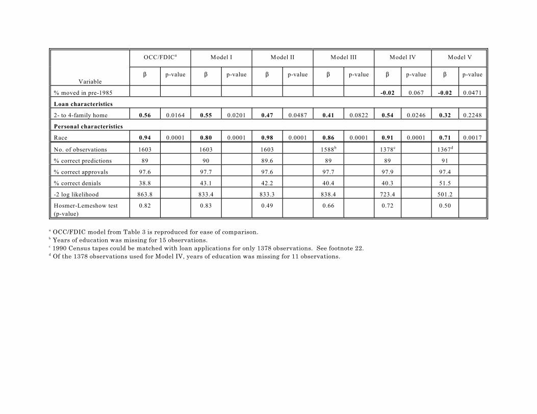
% moved in pre-1985 -0.02 0.067 -0.02 0.0471


2- to 4-family home 0.56 0.0164 0.55 0.0201 0.47 0.0487 0.41 0.0822 0.54 0.0246 0.32 0.2248


Race 0.94 0.0001 0.80 0.0001 0.98 0.0001 0.86 0.0001 0.91 0.0001 0.71 0.0017

No. of observations 1603 1603 1603 1588 1378 1367b c d

% correct predictions 89 90 89.6 89 89 91

% correct approvals 97.6 97.7 97.6 97.7 97.9 97.4

% correct denials 38.8 43.1 42.2 40.4 40.3 51.5

-2 log likelihood 863.8 833.4 833.3 838.4 723.4 501.2

Hosmer-Lemeshow test

(p-value)

0.82 0.83 0.49 0.66 0.72 0.50

OCC/FDIC model from Table 3 is reproduced for ease of comparison.a

Years of education was missing for 15 observations.b

1990 Census tapes could be matched with loan applications for only 1378 observations. See footnote 22.c

Of the 1378 observations used for Model IV, years of education was missing for 11 observations.d

In addition, it is not at all clear how the rent-to-value ratio was derived. The authors state that it can20

be derived from Census tract data, but the Census reports housing values only for owner-occupied housing

units.

The number of units boarded up, the number vacant, a measure of housing value appreciation in recent21

years, the rate of foreclosure, a dummy variable indicating minority population share over 30 percent, and

a set of separate dummy variables for each Census tract.

24

As shown in Table 4, for Model III the dummy variable for self-employed applicantsgrows both larger and considerably more significant. The two new variables are bothnegative, as expected, indicating that the probability of denial is lower for applicantswith more education and with longer experience in their current occupation; bothestimated coefficients are significant. The race coefficient is slightly lower and stillhighly significant. The goodness-of-fit statistic is less than that associated with theBoston Fed specification; however, it still suggests the specification of Model III isquite good. The measures of correct predictions show modest improvement.

The estimated coefficients for the remaining variables, in general, show only slightchanges in magnitude. There was, however, a substantial change in significance levelof the coefficient on the housing debt ratio. The dummy variable indicating a housingdebt-to-income ratio above 30 percent went from about 3 percent significance to about11 percent.

Neighborhood effects. It is widely believed that the location of the property beingpurchased enters into the underwriting decision. In particular, if the home is in anarea where it can reasonably be expected that property values may show little growth,or in fact decline, then a loan is less likely to be approved, all other things being equal,because the probability of default is higher and the position of the mortgagee is lesssecure.

Measuring this location effect, however, has proven to be difficult. The Boston Fedstudy uses a rather unusual proxy variable, the ratio of rental income to the value ofthe rental housing stock in the Census tract where the property is located. Theestimated coefficient was positive, indicating that higher rent-to-value ratios areassociated with higher probabilities of denial. The estimate is highly significant in thepublished results for the full sample, but insignificant in the combined OCC/FDICsample.

The Boston Fed's choice was based on the presumption that landlords demand a higherreturn on riskier properties. While there is some logic to this line of reasoning, theauthors do not present any evidence to support the contention that this ratio is in facthigher in riskier or deteriorating areas, or to prove that any such differential returnsthat might exist are, in fact, due to differences in risk. While the authors did try20

several other measures of neighborhood effects, as reported in the Appendix, there are21

Matching the data proved to be problematic. The 1990 HMDA data reported Census tracts based on22

the 1980 tract definitions, and many tract boundaries were changed for the 1990 Census. Therefore, loan

files could not be matched with the 1990 Census tapes in those cases where the 1980 tract designation was

changed. Since tract-based neighborhood variables could not be defined in such cases, they were dropped

from the analysis. This process resulted in the loss of 225 cases, leaving a sample of 1,378 applications.

While this could potentially lead to biased results, a comparison of the descriptive statistics for the full

OCC/FDIC sample and the reduced sample showed remarkable similarity of means and standard deviations.

25

many other possible candidates that have been used by other authors and that arereadily available from the Census tapes.

After matching the OCC/FDIC sample with 1990 Census tapes, the proportion of22

households who had moved into their residences prior to 1985 was substituted for therent-to-value ratio. The pre-1985 variable can be interpreted as a proxy forneighborhood stability, with the presumption that the more households that stay intheir residences for a long time, the more stable the property values in an area and thelower the default rate and collateral risks to the lender.

As shown in Table 4, for Model IV the estimated coefficient for the new variable,percent moved in pre-1985, is negative, indicating that a location in a more stablen e i g h b o r h o o d l o w e r s t h e p r o b a b i l i t y o f

26

Table 5. Results of regression model: Boston Fed and alternative specification

VariableBoston I.A Model Va

Coefficient p-value Coefficient p-value

Constant -7.2 0.0001 -2.48 0.0052


Housing expense ratio 0.49 0.0371

Excess above 28% 0.0007 0.3430

Total debt ratio 0.05 0.0001

Excess above 36% 0.15 0.0001

Excess above 36% sqd -0.001 0.1345

Net wealth .00009 0.2843 .00008 0.2445

Risk of default

Cons. credit history 0.35 0.0001 0.38 0.0001

Mtg. credit history 0.51 0.0036 0.49 0.0099

Public record history 1.4 0.0001 1.34 0.0001

Prob. unemployment 0.07 0.1402

Self-employed 0.24 0.4094 0.46 0.1389

Yrs. of education -0.10 0.0033

Over 5 yrs. in occ. -0.35 0.1292


Loan-to-value ratio 0.51 0.0051

Excess above 80% 1.76 0.0360

Excess above 80% sqd -0.23 0.0354

Above 90% 0.90 0.0008

Denied PMI 4.87 0.0001 5.02 0.0001

Rent/value in tract 0.23 0.6856

% moved in pre-1985 -0.02 0.0471


2- to 4-family home 0.56 0.0210 0.32 0.2248


Race 0.98 0.0001 0.71 0.0017

No. of observations 1367 1367

% correct predictions 89 91

% correct approvals 97.5 97.4

% correct denials 40.7 51.5

-2 log likelihood 723.4 501.2

H-L test (p-value) 0.50 0.50

Results reported are for the same specification as Boston I, but for a reduced sample size. a

The intercept is also considerably smaller than almost all previous specifications, indicating that the23

new variables are capturing some of the effects that were previously combined in the constant term.

27

denial, as expected.

The estimate is significant at the 10 percent level only, which is marginal, yet farbetter than the virtually total lack of significance for the rent-to-value variable. Inother respects as well, comparison of the alternative to the Boston specificationproduces mixed results. The goodness-of-fit statistic is almost identical. The overallpercent correct predictions is slightly higher, but that is due entirely to a betterperformance predicting approvals, while the percent of correct denials is lower. Therace coefficient is slightly lower and still highly significant. The remaining coefficientsand significance levels showed only slight changes.

Other variables. A number of alternative specifications were also attempted in variousother categories such as gender, age, and marital status; property characteristics (e.g.,condominium and non-owner occupied); types of institutions (e.g., national banks, statebanks, mortgage subsidiaries); and a dummy variable for each separate lendinginstitution. Since these specifications did not substantially alter the outcomes, theyare not reported in detail here.

Alternative specification: Summary. Table 4 presents, as Model V, regression resultsfor a specification combining all of the alternative variables discussed in the precedingsections. The signs of the new variables are all the same as when they were introducedseparately, and the magnitudes are approximately the same as well. The significanceof three of the new variables, however, disappears when they are used in combination:The excess of the housing debt ratio above 28 percent squared, the excess of the totaldebt ratio above 36 percent squared, and the dummy variable indicating more than fiveyears in the same line of work. The coefficient on the race variable is lower than thatin the preceding four models reported in Table 4, and also is lower than the resultswhen the Boston specification is run on the same sample. This indicates that the newspecification is capturing some variation in outcomes that was previously attributedto the race of the applicant. The coefficient for race is still large and positive,23

however, and

28

remains highly significant. Table 5 reproduces the results from Model V and from the Boston Fed specificationestimated for the same sample (1,367 observations) for purposes of comparison. Thetwo specifications have virtually identical goodness-of-fit statistics. The log likelihoodratio for the alternative specification, however, shows very substantial improvement,and the alternative specification does better than the basic model in terms of thepercent correct predictions. Of particular note is the large improvement in the percentof denials correctly predicted, from 40.7 percent to 51.5 percent. Finally, there is littlechange in the signs, magnitudes, or significance levels of any of the other variables.

An examination of the estimated probabilities of denial from the two specifications forindividual applicants reveals that the difference in results from the two models can besubstantial in many cases. For about half of the observations, the two estimatedprobabilities are within two percentage points; for 13 percent of the observations,however, the difference is greater than ten percentage points and,for a few cases itexceeds 40 percentage points. The probabilities estimated by the original Bostonspecification exceed those from the alternative specification for about 60 percent of theobservations; they are smaller for the remaining 40 percent. Further, of thoseapplications that were actually denied and had estimated probabilities of denial of 0.5or less in the Boston model but more than 0.5 in the alternative specification, theamount of increase was generally quite substantial. Thus, the increase in the percentof denials correctly predicted, discussed in the previous paragraph, is not due toprobabilities that went from just slightly below 50 percent to just slightly above thatlevel.

Because of the form of the logit model, it is difficult to deduce the actual impact ofchanges in the independent variables on the probability of denial directly from theregression results. Therefore, Table 6 presents the results of the alternativespecification discussed above in a more readily comprehensible format.

29

Table 6. Impact on probability of denial

Variable

Impact on estimated probability of denial

(percent)

Boston I Model V


Housing expense ratio 33.9 3.8

Total debt ratio 33.0 67.8

Net wealth 4.5 5.0

Risk of default

Consumer credit history 37.2 32.8

Mortgage credit history 11.4 12.9

Public record history 113.7 107.2

Probability of unemployment 11.4

Self-employed 35.1 22.9

Years of education -13.1

Over 5 years in occupation -13.9


Loan-to-value ratio 11.5 78.4

Denied PMI 596.0 609.6

Rent/value in tract 9.3 16.7

% moved in pre-1985 -9.4


2- to 4- family home 42.5 16.7


Race 56.0 49.3

The table shows the percentage change in the average estimated probability of denialas a result of a change in the value of each independent variable. For the dummyvariables, the table shows the impact of the presence of the particular attribute (e.g.,self-employed) relative to an otherwise identical application without the attribute (notself-employed). For the continuous variables, such as net wealth, the table shows the

The methodology employed in constructing the table is the same as that used by the Boston Fed.24

. . . the first step is to determine the probability of denial in the absence of a particular

characteristic, such as being self-employed. This requires determining for each non-self-

employed applicant the probability of denial based on the [estimated] coefficients . . . . These

estimated probabilities for each applicant are then averaged to get a single figure for the

group. The second step is to add to each non-self-employed applicant's probability of denial

the impact of being self-employed (the coefficient . . . multiplied by 1). These new

probabilities are averaged. The figure reported in the [table] . . .

is the percent difference between the average probability of denial for the non-self-employed with

the self-employment effect and the probability for the non-self-employed without it.

For a continuous variable, such as [net wealth] . . . the procedure is slightly different. In this case,

the first step is to determine the estimated probability of denial for each applicant in the sample, and

then average the probabilities. The second step is to add one standard deviation to [net wealth] . .

. for each applicant, recalculate the estimated probabilities of denial, and average the probabilities.

As before, the value reported in the [table] . . . is the percent difference between these two average

probabilities (Munnell et al. 1992, p. 29).

This procedure was modified slightly for the alternative specification in the case of the loan-to-value ratio,

where there are three separate variables based on the ratio (excess above 80 percent, excess above 80 percent

squared, and a dummy variable indicating if over 90 percent). The loan-to-value ratio was increased by one

standard deviation, and all three variables were recalculated; then the new probability of denial was

recalculated for each observation based on the recalculated loan-to-value variables, and the new average was

calculated. A similar procedure was followed for the total debt ratio.

Based on discussions with underwriters, this is a very plausible outcome. Lenders pay much more25

attention to the borrower's total debt burden (relative to income) than to its composition.

30

impact of a one standard deviation change. 24

Most of the variables common to both specifications show little change in their impactson the estimated probability of denial; the one exception is self-employment, whichincreases the average probability only 22.9 percent in the alternative specification,down from 35.1 percent in the original study. As expected, the most significantchanges arise in the cases of the variables that have been transformed in thealternative specification: The total impact of a one standard deviation increase in theloan-to-value ratio has increased dramatically; the housing debt ratio has much lessimpact, while that of the total debt ratio is approximately double what it was before.25

Most importantly, the impact of minority status, although somewhat diminished, isstill quite large: A Black or Hispanic applicant would have, on average, a 49 percentgreater probability of being denied than an otherwise identical white.

Conclusion: Robustness of the race coefficient

The efforts to develop alternative specifications for the model were fruitful in terms ofthe results for individual variables and groups of variables that seemed, a priori, to

For example, we had serious reservations about the particular way that credit history was modeled by26

the Boston Fed. However, it was not possible to explore alternative formulations of this important variable,

because the credit history variables contained in the data provided by the Boston Fed were already coded

in the precise form used in the Boston study. Therefore, any effort to model different kinds of credit history

effects will have to await collection of new data for future studies. Also, see discussion in Section VI under

Model misspecifications and omitted variables in the text for other specification issues that could not be

investigated with the data made available by the Boston Fed.

31

better approximate the mortgage underwriting process, as well as in terms of improvedpredictive ability. Nonetheless, the one result of the Boston study that has attractedthe most attention and that has the strongest public policy implications, the estimatedcoefficient for the race variable and its significance, remains highly robust acrossspecifications. Through many dozens of alternative specifications, both those reportedabove and many others not reported, the coefficient is always positive, within a narrowrange (most often between 0.7 to 0.9), and very highly significant. At least with thealternative specifications that could be explored with the data provided by the BostonFed, we could not refute the Boston Fed's conclusion that mortgage lenders in the26

Boston MSA, collectively, treated Black and Hispanic applicants differently fromwhites in 1990, and that, on average, a Black or Hispanic applicant had anapproximately 50 percent greater probability of being turned down than a whiteapplicant with otherwise identical characteristics.

Of course these results are valid only insofar as the data truly reflects the underlyingpopulation. Several recent articles have suggested that the Boston Fed data iscontaminated by numerous data errors and inconsistencies. They argue these errorscould significantly influence the outcome of the Boston Fed study. In the next section,we address many of these issues.

VI. Data entry/reporting errors

The Boston Fed states that they subjected the data to "careful visual inspection andcomputer edits and repeatedly called back lenders to verify that data items thatseemed unusually large or small actually reflected the contents of the lenders' files"(Browne 1993). There are, however, numerous instances in the partial data setsprovided to the OCC and FDIC by the Boston Fed in which the data remain suspect.We discuss several examples of data errors we found in the OCC/FDIC data and theimplications those errors may have for the Boston Fed's results.

Analyzing the impact of data errors and inconsistencies Duplicate files and coding errors. Several of the more obvious data entry errors wereeasily corrected. For example, duplicate files were dropped from the data set, and thedebt obligation ratios entered as decimal values were converted to percentages. Thereare relatively few of these errors, and correcting them resulted in no substantive

For example, one approved applicant with an annual income of $89,544 had negative net wealth of27

almost $2 million, yet reported total non-housing debt payments of only $156 per month. This is an

unreasonably low monthly debt payment. Using a monthly payment rule-of-thumb of .005, this person

should have a non-housing monthly debt payment of approximately $10,000.

Even under the assumption that the rates used to calculate the proposed monthly housing payment28

were "teaser" rates on adjustable-rate loans (though many of them are coded as fixed-rate mortgages), the

underwriting decision should have been based on a "qualifying" rate that reflects the then-current market

rate on fixed-rate mortgages. Day and Liebowitz (1993) also discuss this apparent data entry error.

One suggested solution would involve deleting these files from the data set. However, we believe this29

is inappropriate because the remaining sample may well be unrepresentative of the underlying population,

thus introducing sample selection bias that will distort the estimates in an unknown manner.

32

change in the Boston Fed's conclusions. It is not surprising these errors had so littleimpact on the results given that there is relatively low leverage associated withextreme values in logit models (a statistical property of the estimating procedure), sothat even large changes in these values (i.e., converting the debt ratio from a decimalto a percent) can have very small effects on the parameter estimates.

Correcting for other data entry problems, however, is more problematic. Often it isdifficult to know if the correction itself introduces more error; and deleting theobservation may bias the sample if the errors are non-random across groupings.Moreover, for errors of inconsistency it is difficult to determine which data are false;therefore, the method used to correct the errors may substantially influence theresults. We discuss several of these problems below.

Inconsistencies that suggest the debt ratios are underreported. It is likely, given thelarge number of files with monthly non-housing debt payments far below thoseconsistent with the level of outstanding liabilities, that the total debt obligation ratiois underreported in many files. Moreover, the proposed monthly housing payments27

for another 3 percent of the applicants were below that required on a loan with a 6percent mortgage interest rate (at a time when market rates were above 10 percent).This suggests that both the monthly housing expense ratio and the total debt ratiowere underreported for these observations as well.28

In these cases, the applicant may appear qualified according to the model (that is,assigned a low estimated probability of denial), yet appear unqualified to theunderwriter, based on accurate information concerning housing and non-housing debtpayments. Errors of this type reduce the reliability of the model in general, and theimportance of the housing expense and total debt obligation ratios specifically asindicators of loan disposition. There is no obvious way these errors can be correctedshort of re-examining the loan files; a solution we believe is impractical.29

Including unverified data. Two types of data verification errors are introduced in the

FDIC examiners found that several institutions reported information from the original (unverified)30

application, not from the final application, even though the original data are not necessarily used to make

the loan decision (Horne 1994).

In many cases, income, assets, and debt obligations are modified during the verification period. This31

is especially true of income. Expected raises, part-time income, child support, interest income, annual bonus

and over-time income, a sudden change in income, etc. that are normally reported at the time of initial

application may often be either reduced or not counted (though they may be used as a compensating factor)

by the underwriter. Moreover, the non-housing expenses listed on the initial application may be incomplete;

they are often adjusted using the information from the applicant's credit report.

33

Boston Fed study: (i) several banks reported data from the unverified, initialapplication, and (ii) several applications contained information provided by the30

borrower that was not (or could not be) verified by the bank. Both of these dataverification problems are especially troublesome for it is difficult to know, a priori, howsensitive the coefficient of the race variable is to these errors.

For example, including unverified data from the original, rather than the final,application form may significantly affect the model's results if the unverified data tendto overstate the qualifications of marginal borrowers (i.e., if the financial and credithistory characteristics of the denied applicants appear to approach those of theapproved applicants). The overstated qualifications of marginal borrowers reduce the31

model's ability to accurately identify the importance of each explanatory variable in thelending decision. If the unverified data from the original applications enterdisproportionately from a single race category, a model that relies on a single(categorical) variable to proxy for the race effect may wrongly attribute the differencein denial rates to race. The difference in denial rates will be more accurately reflectedby differences in financial and credit history characteristics of the applicant if the dataused in the model more accurately reflect the differences in qualifications. The greaterthe difference between the actual (verified) data and the reported data, the more likelythe results of the statistical model will be misleading. Verification errors of this typeare impossible to correct without re-examining the loan files.

Data verification errors introduced by failing to incorporate information about theability of the bank to verify all (relevant) information on the application are lesstroublesome to correct. The Boston Fed data set contains an indicator variable (N56 -unverifiable information) that may reduce the bias associated with overstatedunverified data. This variable identifies loan applications containing credit,employment, income, residence, or "other" information that could not be (or was not)verified by the loan officer. Interestingly, unverified information was not necessarilya fatal derogatory characteristic (see Table 7). However, minorities with unverifiedinformation were 70 percent more likely to be denied than whites with unverifiedinformation.

It is also interesting to note that of the 100 files that are identified as having unverified information,32

half are minority applicants. That is, only 4.1 percent of the white applications have unverified information,

while nearly 14 percent of the minorities do. Moreover, 26 of the 50 white applicants with unverified

information (52 percent) were approved, but only 9 of the 50 minorities (18 percent) were.

34

Table 7. Loan Files with Unverified Data by Race and Loan Disposition

Approved Denied Percent

denied

Non-minority 26 24 48

Minority 9 41 82

Total 35 65 65

The Boston Fed data set identifies four categories of information that could not beverified: credit references, employment, income, and residence. We tried severalmethods of incorporating the unverified information dummy variable into the BostonFed model. We found the results to be sensitive to the method used (see Table 8);however, the magnitude and significance of the race coefficent are not affected.Including the unverified information variable increases the explanatory power of themodel, suggesting either (i) the probability of denial increases if vital information isnot verified by the bank, or (ii) loan officers tend not to verify information if the initialqualifications of the applicant are so poor that approval seems unlikely. It is not clearfrom the data if either or both of these are driving the result. It is interesting to note,however, that roughly 37 percent of the minority denials have unverified data, ascompared to only 21 percent of the majority denials. We return to this issue below.32

35

Table 8. Results of regression model: Unverified Information

Variable

Coefficient

(p-value)

Model VI Model VII

Constant -6.82

(0.0001)

-6.6

(0.0001)

Housing expense ratio 0.41

(0.0804)

0.35

(0.1241)

Total debt ratio 0.042

(0.0001)

0.035

(0.0001)

Unverified Income and "Other"

x Debt Ratio

0.073

(0.0001)

Net wealth 0.0001

(0.1723)

0.0001

(0.1534)

Consumer credit history 0.34

(0.0001)

0.33

(0.0001)

Mortgage credit history 0.41

(0.0209)

0.48

(0.0047)

Public record history 1.37

(0.0001)

1.41

(0.0001)

Probability of unemployment .071

(0.1017)

0.065

(0.1306)

Self-employed 0.47

(0.0867)

0.41

(0.1306)

Loan-to-value ratio 0.46

(0.0136)

0.51

(0.0050)

Denied private mortgage insurance 4.42

(0.0093)

4.43

(0.0001)

Rent/value in tract 0.59

(0.0167)

0.62

(0.0107)

Purchasing 2- to 4-family home 0.22

(0.6508)

0.18

(0.7036)

Race 0.85

(0.0001)

0.90

(0.0001)

Unverified information 2.45

(0.0001)

Number of observations 1601 1603a

Percent correct predictions 91.3 90.6


The unverified information variable was missing for two observations.a

36

Sufficient funds to close. Having sufficient "funds to close" (that is, to cover thedownpayment, closing costs, and two months' payments) is a virtually universalunderwriting requirement, and lack of sufficient funds is often cited as a reason fordenial. The handling of this criterion in the Boston Fed model, however, isproblematic, and may not fully capture its impact on the lending decision.

In the Boston Fed model, the downpayment amount is reflected in the loan-to-valueratio, which proves to be a consistently important and significant variable. In addition,the model attempts to capture the sufficiency of funds to close through the use of netwealth and, alternatively, liquid assets. Neither of these latter variables, however,turns out to be significant, a result which, according to the authors, appears "to supportlenders' claims that they do not place much weight on wealth . . . . Pre-screening mayalso exclude people without enough cash to settle" (Munnell et al. 1992, p. 30).

These explanations notwithstanding, it still seems curious that some measure of fundsto close

In addition, the value listed for furniture and personal property is notoriously arbitrary and inflated.33

37

does not have significant explanatory power in the final model, in particular in lightof the fact that coming up with a downpayment has been found to be the primaryobstacle to homeownership for millions of American households (Apgar et al. 1990,Horne 1994). On closer examination, however, the treatment of this issue in theBoston model may be inadequate for several reasons. First, no attempt is made tomeasure available assets relative to the amount of money needed to close. Second, thevarious fees and points that must be paid by the buyer at closing are not taken intoaccount; these can often constitute a substantial amount, especially for a marginalapplicant or first-time buyer who is struggling to come up with the necessary funds.And finally, the way that equity in a present home and gifts or grants were handledraises questions about the ability of the model to fully capture the "funds to close"standard.

While the amount of equity in a present home should, in principle, be captured in networth, it is likely that the net worth variable is misleading and inaccurate in thiscontext. Net worth includes, among other things, real estate owned (which mayinclude properties other than the current home), net worth of businesses owned, autos,and furniture and personal property. From the total assets figure it is impossible todistinguish the amount of equity in the current home (which is generally to be sold tomove into the new home) from other assets the applicant may neither desire nor be able to liquidate in order to cover the closing costs of the newhome.33

There are similar questions with regard to gifts or grants used to meet part of thedownpayment and closing costs. The data questionnaire in the Boston study includedan item, "Did a gift or grant account for any part of the down payment?" and a dummyvariable reflecting the answer was included in the model. The estimated coefficientindicated a lower probability of denial for applicants who had received gifts or grants,but it was not significant. To the extent that gifts actually received are accuratelyreflected in liquid assets, net wealth, downpayment amount, and the loan-to-valueratio, this result, by itself, is not a cause for concern. In fact, it is consistent withlenders' contentions, as cited in the Boston Fed study (Munnell et al. 1992, pp. 14 and30), that wealth is not a significant factor in their decision-making.

However, it is possible that the net wealth and liquid assets data do not accuratelyaccount for gifts received. Often, for example, gifts are received just prior to closing,and the amount of the anticipated gift may not be included in the liquid assets reportedon the application form. This problem is even more likely to occur in those cases wheredata for the study was taken from the initial, rather than the final, application form(Horne 1994, p. 7). FDIC examiners also found instances where gifts were indicatedin the loan file, but not verified or received (Horne 1994, p. 11). These findings raise

Without knowing how the occurrence of the two situations cited in the text is correlated with race, it34

is not possible to speculate, a priori, on the sign or magnitude of the effect that of any such bias might have

on the estimated coefficient of the race variable.

This type of misspecification can seriously affect the results of a regression analysis, resulting in biased35

and inconsistent estimators (even if the omitted variables are uncorrelated with race). This implies that, not

only are the magnitudes of the coefficients wrong (i.e., biased), but the usual tests of significance are no

longer valid. See Lee (1982) and Kmenta (1986).

We separate the analysis of these two variables from the earlier discussion in Section V, Alternative36

specifications, because of the measurement problems associated with these variables. The special loan

programs series has numerous errors. Adjustable-rate, FHA, VA, conventional, jumbo, balloon, and

construction loan are incorrectly identified as special programs by several of the banks. Moreover, loans

made to finance the purchase of other real estate owned by the bank (OREO) were also included in this

category. Since all of these applications are obviously misclassified as special loan programs, we excluded

38

two possibilities: that a gift actually received was not reflected in reported liquidassets, or that a gift included in reported liquid assets was ultimately never received.In either case, the Boston Fed model would fail to accurately capture the effect of thegift, or its absence, and the results of the model may be biased as a consequence.34

The inability of the Boston model to accurately measure the true amount of assetsavailable to cover closing costs may explain the insignificant results obtained for netwealth and liquid assets. Further, it means that denials that arise entirely, or in largepart, because of insufficient funds may be attributed by the model to other factors. Asexamples, if minorities are disproportionately less likely to be current homeowners orif, as homeowners, they tend to have less equity in their homes, or if they aredisproportionately more likely to report anticipated gifts that fail to materialize, theseproblems would result in an upwardly biased estimate of the race coefficient.

We attempted to better capture the issue of sufficient funds to close, with a variablerepresenting the ratio of liquid assets to closing costs (defined for this purpose as thedownpayment plus two months' proposed housing costs); the results were notsignificant. However, this may well have been due to the measure used and to theproblems with the Boston data. To explore this issue adequately, it would be necessaryto collect data on the aspects of financial ability not included in the Boston Fed'squestionnaire: verification and actual receipt of gifts or grants, equity in a currenthome, and the amount of other closing costs (fees, points, etc.)

Model misspecification and omitted variables

The model has also been criticized for failing to include several relevant decisionvariables that are correlated with race, which implies that the model has omittedvariable bias. Of particular interest, given the Boston Fed data, is the inclusion of35

information on special programs and program guidelines.36

them from our sample of applications made under a special loan program.

The program guidelines series has been criticized as inconsistent across institutions by the Boston Fed

because the variable was not adequately defined. There may be some merit to their concern. However,

although the instructions to the banks were ambiguous, the data suggest that banks did not systematically

report that all loans denied failed to meet program guidelines. We suspect most banks cited failure to meet

guidelines if the application was denied for credit history problems. Still, it is unknown whether the variable

is derived using general (i.e., secondary market) guidelines, bank-specific guidelines, or program-specific

guidelines.

The Boston Fed reports (Munnell et al. 1992, pp. 52 and 63) that they tried, unsuccessfully, to37

incorporate a dummy variable for special programs into their model. However, their lack of success is most

likely attributable to the data problems associated with this variable, as discussed in the previous footnote.

39

Many mortgage lenders are developing special loan programs to assist first timehomebuyers and "other" specially qualified applicants (such as individuals who areunable to make a nominal downpayment in spite of strong financial/credit histories);or are participating in programs developed by the Federal National MortgageAssociation (Fannie Mae), the Federal Home Loan Mortgage Corporation (FreddieMac), or state or local government agencies. The presumption is that the underwritingcriteria applied to these loan applications are different from those applied toconventional loan applications. The Boston Fed data set pools applications withoutrespect to whether they participate in a special program. This may result in acomparison of loan applications with very different underwriting standards.Accordingly, we would have expected the model to include a special loan programvariable which would capture the change in the weights applied to those applicationsmade under a special loans program.

The results of the statistical model may be biased if the special loan programinformation is ignored, especially if a disproportionate share of one racial groupparticipated in special programs. (This is true with the Boston Fed's sample, whereover 50 percent of minority applicants ) 51 percent of approvals and 55 percent of thedenials ) applied under a special loan program, as compared to only about 13 percentof the white applicants ) 12.8 percent of approvals and 18.8 percent of denials.)Because the Boston Fed model does not include a special loan program variable, therace coefficient may capture the effect associated with the difference in underwritingstandards, not just the difference in treatment due to race.37

A special program indicator by itself may not adequately capture the impact of lessstringent underwriting standards. Interaction variables are used instead of a singleindicator variable to separate out the effects of the special loan programs' underwritingstandards on debt ratios, credit history, and loan-to-value ratio. The special loanprogram variables are, in general, of the right sign and are statistically significant (seeTable 9 - Model VIII). All else being equal, a borrower who applies under a specialprogram will tend to have a lower probability of denial. However, the sign on the total

40

debt-to-income interaction variable suggests underwriters are more concerned abouta borrower's total debt burden when the borrower is applying under a special program.An applicant applying under a special loan program with high debt levels has a higherprobability of denial. (This result is consistent with special loan programs found atmany lending institutions today, such as first-time homebuyers programs, that allowvery high loan-to-value ratios but generally are strict on debt ratios and recent credithistory.)

Though the inclusion of controls for special programs increases the explanatory powerof the model relative to the basic Boston specification (see Table 4), the impact on therace variable is small. Moreover, the goodness-of-fit falls dramatically. Though thecoefficients of the model are plausible, the low p-value for the Hosmer-Lemeshow testsuggests the accuracy of the model is only marginal.

A related model misspecification issue concerns the failure to incorporate informationon the credit guidelines used by the bank to evaluate the loan application.Misspecification may exist due to (i) differences in underwriting standards acrossbanks (some banks may be more flexible

41

Table 9. Results of regression model: Special Loans Programs and ProgramGuidelines

Variable

Model VIII Model


Constant -6.88 0.0001 -1.00 0.0413


Housing expense ratio 0.59 0.0099 0.68 0.0124

Total debt ratio 0.035 0.0001 0.027 0.0045

Net wealth 0.00008 0.2568 -0.00001 0.8924

Risk of default

Consumer credit history 0.36 0.0001

Mortgage credit history 0.48 0.0038

Public record history 1.25 0.0001

Probability of unemployment 0.06 0.1235 0.04 0.3932

Self-employed 0.40 0.1278 0.66 0.0301


Loan-to-value ratio 1.00 0.0070 0.55 0.0597

Denied private mortgage insurance 4.56 0.0001 4.41 0.0001

Rent/value in tract 0.59 0.0121 0.73 0.0084


Purchasing 2- to 4-family home 0.12 0.8109 0.22 0.7071

Total debt ratio x spec. pgm. 0.079 0.0005 0.11 0.0006

Mort. credit history x spec. pgm. -0.10 0.2974 -0.18 0.1073

Housing exp. ratio x spec. pgm. -0.07 0.0581 -0.11 0.0070

Loan-to-value ratio x spec. pgm. -0.97 0.0373 -0.48 0.2145


Race 0.92 0.0001 0.74 0.0030

Meets guidelines -4.12 0.0001

Number of observations 1603 1601a



The "meets guidelines?" question was not answered ) either yes or no ) for two observations.a

than others, especially if they anticipate selling the mortgage), (ii) banks rejecting wellqualified applicants that are overqualified under special program guidelines (see Horne1994), and (iii) banks approving marginally to poorly qualified applicants under theless stringent, special program qualifying standards.

42

Table 10. Results of regression model: Unverified data and special loan programs

Variable

Model X Model XI


Constant -1.42 0.0046 -1.07 0.0293


Housing expense ratio 0.59 0.0375 0.64 0.0192

Total debt ratio 0.029 0.0028 0.028 0.0034

Net wealth 0.000007 0.9396 -0.000009 0.9192

Risk of default

Probability of unemployment 0.046 0.3532 0.04 0.4317

Self-employed 0.74 0.0155 0.707 0.0193


Loan-to-value ratio 0.54 0.0716 0.54 0.0651

Denied private mortgage insurance 4.27 0.0001 4.34 0.0001

Rent/value in tract 0.75 0.0094 0.78 0.0057


Purchasing 2- to 4-family home 0.23 0.6847 0.15 0.7934

Total debt ratio x spec. pgm. 0.094 0.0094 0.09 0.0113

Mort. credit history x spec. pgm. -0.14 0.2204 -0.12 0.3053

Housing exp. ratio x spec. pgm. -0.09 0.0478 -0.094 0.0442

Loan-to-value x spec. pgm. -0.65 0.1232 -0.69 0.0987


Race 0.68 0.0094 0.42 0.1248

Meets guidelines -3.91 0.0001 -4.03 0.0001

Unverified information 2.01 0.0001

Unverified info. x minority 2.52 0.0001




Ideally, loan applications should be matched directly with the guidelines used toevaluate the credit quality of the borrower. Discrimination would exist if theguidelines were applied unfairly across racial groups. Unfortunately, this informationwas not collected for the Boston Fed study. The Boston Fed did, however, request thatthe banks indicate if the applicants' credit histories met the bank's loan policy

It is important to note that the survey question applied to credit history only, not to all the guidelines38

for the loan program under which the application was submitted. Moreover, it is unclear exactly what this

variable measures, even in the case of credit history. We expect the variable is used in most cases to indicate

if the application was denied for credit history problems. It is unknown whether the variable is derived using

general (i.e., secondary market) guidelines, bank-specific guidelines, or program-specific guidelines. That

is, were all loan applications subject to the same underwriting standards, or were some applications given

special consideration under a special loan program?

Applications rejected as overqualified for special programs cannot be identified solely from the data and,39

therefore, cannot be dealt with in the same manner.

Day and Liebowitz (1993) include the "meets guidelines" variable in their model. They also found it40

explains a large portion of (but does not eliminate) the difference in denial rates across racial groups. They

proceed to partition the sample into finer groups, by property type. Although we believe there may exist

differences in underwriting standards by property type, we are concerned that further partitioning the data

creates subsamples that no longer represent the population and, therefore, introduce additional selection

bias. We believe, however, that additional research is needed to address this issue.

43

guidelines for approval. We use the "meets guideline" variable to partially address38

the types of misspecification discussed in (i) and (iii). The results are reported in39

Table 9 as Model IX. The coefficient on the race variable is significantly reduced butis not eliminated after controlling for credit history guidelines. This model, however,40

performs poorly.

We combined the effects of unverified information, special programs, and programguidelines and report the results in Table 10. The coefficients for both the unverifiedinformation and the meet guidelines variables are statistically significant. However,the model performs poorly as indicated by the very low Hosmer-Lemeshow statistic(see Model X). Modifying the unverified information variable by replacing it with aninteraction term between race and unverified information significantly improves themodel's goodness-of-fit (see Model XI). More interestingly, the coefficient on the racevariable is no longer significantly different from zero. This suggests minorityapplicants are treated the same as majority applicants, except those with unverifiedinformation. The difference in the denial rates is explained by the differences inhousing expense ratio, total debt ratio, credit history, loan-to-value ratio, denied PMI,and meets guidelines.

The results of Model XI certainly do not prove that discrimination did not exist in theBoston mortgage market in 1990. The fact that Model XI is the only specification, outof dozens attempted, where race is not significant is probably more important than thelack of significance itself; this is particularly true given the numerous problems,discussed above, with all three of the variables (unverified information, specialprogram, and meets guidelines) used in this model.

Given the problems with the variables, and in the context of all the other specificationswhere race was so consistently significant and robust, it is probably more accurate to

44

characterize Model XI as demonstrating that it is always possible, with sufficienteffort, to find some formulation that eliminates the significance of virtually anyvariable in virtually any model. Moreover, Model XI may even suggest an alternativehypothesis that discrimination may still exist, but in a different form. That is, giventhat a large percentage of the denied minority applicants had unverified informationin their files, there may be a racial disparity in the "quality of assistance" given tominority applicants. Loan officers may spend more time working with white applicantsthan with minorities to assure that they submit the documentation necessary to verifyall the information in their files. If that is the case, the lack of verified information maybe masking this more subtle form of discrimination. In any case, the strongestconclusion that can be drawn from Model XI is that this is an area that needs to belooked into more carefully in future research.

VII. Conclusions

Was the Boston Fed right? Most of the commentary and controversy over the BostonFed study has focussed on the central conclusion. Was there really significantdiscrimination against minorities in the mortgage lending market in Boston in 1990?Or, do the data and methodological shortcomings of the study so undermine thevalidity of the results as to cast doubt on the existence of discrimination?

The results of our analysis of the Boston Fed's methodology and data permit us toanswer the first question with only a qualified yes. To the extent that we could correctthe most obvious data problems, explore alternative specifications, and subject themodel to additional econometric tests ) that is, going as far as was possible using theBoston data ) the model overall and the race coefficient in particular were remarkablyrobust. Our results could not refute the findings of the Boston Fed concerningdifferences in treatment between minorities and whites. The coefficient on the racevariable remains statistically significant and of approximately the same magnitude asthat found in the original study.

However, as pointed out above, there were numerous data errors that could not bereadily corrected and alternative specifications that could not be tested with theavailable data. Thus, it is not possible to definitively reaffirm, or to repudiate, theresults of the Boston Fed study. The only way to do so would be to go back to theoriginal loan files at all 131 participating institutions to verify the original data,correct data errors, and collect data on additional variables (or different forms of somevariables). However, given the intense publicity and controversy generated by therelease of the Boston Fed study, as well as the federal and state enforcement actionsthat have ensued as a direct consequence of the study, it is virtually certain that sucha follow-up effort will never take place.

Where do we go from here? While setting the record straight once and for all about the

45

Boston Fed study would certainly be important for its own sake, the impossibility ofdoing so does not necessarily affect the research agenda in this area. Even if theBoston study were completely beyond reproach in the unanimous opinion of theresearch community, it still represents only one study, in one city, at one point in time.As such, it calls out for replication in other times and places. We should be careful notto draw conclusions about the existence or pervasiveness of discrimination in mortgagelending until and unless we find consistent and systematic evidence in repeatedstudies.

Moreover, in the process of carrying out other studies, researchers can extend andmodify the Boston Fed methodology in two important respects. First, we can learnfrom their problems and shortcomings and can make every attempt to avoid the dataproblems, for example, and to collect data on additional variables. Second, we canexplore the possibility of adapting the econometric methodology to requirements of theexamination procedures employed by the federal bank regulators, in order to developa statistical tool that can assist bank examiners in detecting the existence ofdiscrimination in any single lending institution.

These tasks will constitute the principal objectives of the next phase of our research.

Appendix 1. Key characteristics of mortgage applicants, by race and loan disposition Full Boston sample (3,062 observations) and OCC/FDIC sample (1,603 observations)

Variable

White Black/Hispanic

Approved Denied Approved Denied

Boston OCC/FDIC Boston OCC/FDIC Boston OCC/FDIC Boston OCC/FDIC


Housing expense/income (%) 26.0 26.0 26.6 26.0 26.0 26.0 28.0 29.0a

Total debt/income (%) 33.0 32.5 37.0 37.0 34.0 34.0 38.0 38.0a

Net wealth ($000) 93 94 75 59 39 37 33 29a

Monthly base income

(applicant plus coapplicant) ($)a

4,666 4,691.5 4,471 4,260 3,333 3,412 3,600 3,254

Liquid assets ($000) 38 40 28 23 19 18.75 15.5 13.85a

Risk of default

Percent with poor credit history 14.6 12.7 38.9 41.9 23.4 21.4 51.5 50.4b

Probability of unemployment 3.2 3.2 3.2 3.6 3.2 3.2 3.2 3.2a

Percent self-employed 12.0 12.9 22.4 21.4 7.5 7.6 7.4 6.9


Loan-to-value (%) 77.3 75.1 83.1 83.5 85.0 84.3 90.0 89.7a

Rent/value in tract (%) 4.6 4.6 4.9 5.1 7.3 7.2 8.9 9.1a

Percent applied for PMI 21.6 22.2 17.1 23.9 42.2 42.0 26.6 36.5

Percent denied PMI 0.7 0.8 75.0 82.0 1.3 1.8 82.5 73.8c

Variable

White Black/Hispanic

Approved Denied Approved Denied

Boston OCC/FDIC Boston OCC/FDIC Boston OCC/FDIC Boston OCC/FDIC


Percent purchasing 2- to 4-family home 7.7 7.8 18.3 19.6 24.8 24.8 34.4 31.3

Percent fixed-rate loans 68.6 60.7 62.8 56.4 60.6 46.6 69.6 63.5

Percent 30-year fixed-rate loans 85.9 87.5 83.3 82.9 91.1 94.3 91.3 95.6

Percent in special loan programs 12.6 12.8 16.1 18.8 40.6 50.0 40.3 54.8


Age 34.0 34.0 35.0 35.0 36.0 36.0 36.0 37.0a

Percent married 63.0 61.7 53.2 54.7 53.7 57.2 55.0 50.0

Percent with dependents 37.6 35.5 39.9 42.7 52.6 55.0 52.2 46.1

Median value. a

Poor credit history is defined as more than two late mortgage payments or delinquent consumer credit histories (more than 60 days past b

due) or bankruptcies or other public record defaults.

Based on number applying for private mortgage insurance. c

48

Appendix 2. Variable Definitions

Housing expense ratio Equals 1 if proposed monthly housingpayment to income ratio is greater than.30; otherwise equals 0.

Excess above 28 percent Equals proposed monthly housingpayment to income ratio minus .28 if theresult is positive; otherwise equals 0.

Total debt ratio Equals total monthly debt paymentdivided by monthly income.

Excess above 36 percent Equals total debt ratio minus .36 if theresult is positive; otherwise equals 0.

Excess above 36 percent squared Equals total debt ratio minus .36 if theresult is positive, squared; otherwiseequals 0.

Net wealth Equals total assets minus totalliabilities.

Consumer credit history Equals 1 if no "slow pay" accounts, 2 ifone or two slow pay accounts, 3 if morethan two slow pay accounts, 4 ifinsufficient credit history, 5 if accountshows delinquent credit (60 days pastdue), and 6 if account shows seriouslydeliquent credit (90 days past due).

Mortgage credit history Equals 1 if no late payments, 2 if nopayment history, 3 if one or two latepayments, and 4 if more than two latepayments.

Public record history Equals 1 if any public record of credithistory; otherwise equals 0.

Probability of unemployment Equals the 1989 Massachusettsunemployment rate for the applicant'sindustry.

Self-employed Equals 1 if the applicant is self-employed; otherwise equals 0.

Loan-to-value ratio Equals the loan amount divided by theappraised value.

49

Excess above 80 percent Equals the loan-to-value ratio minus .80if the result is positive; otherwise equals0.

Excess above 80 percent squared Equals the loan-to-value ratio minus .80if the result is positive, squared;otherwise equals 0.

Excess above 90 percent Equals 1 if loan-to-value ratio is greaterthan .90; otherwise equals 0.

Denied private mortgage insurance Equals 1 if the applicants applied forand were denied private mortgageinsurance; otherwise equals 0.

Rent/value in tract Equals rental income divided by value ofrental housing stock in the Census tractin which the property is located.

Purchasing 2- to 4-family home Equals 1 if the applicant is purchasing atwo- to four-family home; otherwiseequals 0.

Race Equals 1 if the applicant is Black orHispanic; otherwise equals 0.

Years of education Equals the number of years of educationfor the applicant (if there is acoapplicant, equals the number of yearsof education for the person with thegreater base monthly income fromwages.

Over five years in occupation Equals 1 if the applicant has been in therecorded line of work more than fiveyears; otherwise equals 0.

Percent moved in pre-1985 Equals the number of households in theCensus tract that moved in before 1985divided by the total number ofhouseholds in that tract that report adate moved in.

50

Unverified informationIncomeEmploymentCredit ReferencesResidenceOther

Equals 1 if reported information couldnot be verified by the underwriter (anaggregate and individual verificiationseries were created for income,employment, credit, residence, andother); otherwise equals 0.

Special program Equals 1 if the applicant applied undera special loan program; otherwise equals0.

Meets guidelines Equals 1 if the applicants' credit historymet the lender's loan policy guidelinesfor approval; otherwise equals 0.

51

References

Apgar, William C., Denise DiPasquale, Jean Cummings, and Nancy McArdle. 1990.The State of the Nation's Housing. Cambridge, Massachusetts: Joint Center forHousing Studies, Harvard University.

Berkovec, James, Glenn Canner, Stuart Gabriel, and Timothy Hannan. 1993. "Race,Redlining, and Residential Mortgage Defaults: Evidence from the FHA-InsuredSingle-Family Loan Program." U.S. Department of Housing and UrbanDevelopment, Home Mortgage Lending & Discrimination: Research andEnforcement Conference. May 18-19.

Berndt, Ernst R. 1991. The Practice of Econometrics: Classic and Contemporary.Reading, Massachusetts: Addison-Wesley Publishing Company.

Blinder, Alan S. 1973. "Wage Discrimination: Reduced Form and StructuralEstimates." The Journal of Human Resources. vol. 18, pp. 436-455.

Browne, Lynn E. 1993. "Boston Fed Study Shows Race Bias." The Wall StreetJournal. September 21.

Day, Ted, and S.J. Liebowitz. 1993. "Mortgages, Minorities, and Discrimination."School of Management, University of Texas at Dallas. Unpublished manuscript.

Horne, David K. 1994. "Evaluating the Role of Race in Mortgage Lending." FDICBanking Review. Forthcoming.

Hosmer, David W., Jr. and Stanley Lemeshow. 1989. Applied Logistic Regression.New York: John Wiley & Sons.

Judge, George G., W.E. Griffith, R. Carter Hill, Helmet Lütkepohl, and Tsoung-ChaoLee. 1990. The Theory and Practice of Econometrics, 2nd ed. New York: JohnWiley & Sons.

King, A. Thomas. 1980. "Discrimination in Mortgage Lending: A Study of ThreeCities." Federal Home Loan Bank Board, Research Working Paper No. 91.February.

Kmenta, Jan. 1986. Elements of Econometrics. New York: Macmillian PubllishingCompany.

52

Lee, L.F. 1982. "Specification Error in Multinomial Logit Models: Analysis of theOmitted Variable Bias." Journal of Econometrics, vol. 20, pp. 197-209.

Liebowitz, Stan. 1993. "A Study That Deserves No Credit." The Wall Street Journal.September 1.

Maddala, G.S. 1983. Limited-Dependent and Qualitative Variables in Econometrics.Cambridge, England: Cambridge University Press.

Munnell, Alicia H., Lynn E. Browne, James McEneaney, and Geoffrey M.B. Tootell.1992. "Mortgage Lending in Boston: Interpreting HMDA Data." FederalReserve Bank of Boston, Working Paper No. 92-7. October.

Perle, Euguene D., Kathryn Lynch, and Jeffrey Horner. 1993. "Model Specificationand Local Mortgage Market Behavior." American Real Estate and UrbanEconomics Association Meeting, Washington, D.C. June 1.

Schafer, Robert and Helen F. Ladd. 1981. Discrimination in Mortgage Lending. MIT-Harvard Joint Center for Urban Studies. Cambridge, Massachusetts:Massachusetts Institute of Technology Press.

Schill, Michael H. and Susan M. Wachter. 1993. "A Tale of Two Cities: Racial andGeographic Disparities in Home Mortgage Lending in Boston and Philadelphia."American Real Estate and Urban Economics Association Meeting, Washington,D.C. June 1.

Siskin, Bernard R. and Leonard A. Cupingood. 1993. "Use of Statistical Models toProvide Statistical Evidence of Discrimination in the Treatment of MortgageLoan Applicants: A Study of One Lending Institution." U.S. Department ofHousing and Urban Development, Home Mortgage Lending & Discrimination:Research and Enforcement Conference. May 18-19.

Van Order, Robert, Ann-Margret Westin, and Peter Zorn. 1993. "Effects of the RacialComposition of Neighborhoods on Default and Implications for RacialDiscrimination in Mortgage Markets." Federal Home Loan MortgageCorporation. March.

Zandi, Mark. 1993. "Boston Fed's Bias Study Was Deeply Flawed." The AmericanBanker. August 19.

an evaluation of the federal reserve bank of boston's study of … · i an evaluation of the...

Documents