An Evaluation of Inferential Procedures forAdaptive Clinical Trial Designs with Pre-specified

Rules for Modifying the Sample SizeGregory P. Levin, Sarah C. Emerson, & Scott S. Emerson

Cesar Torres

June 3, 2014

1

Overview

I Review

I Distribution of sampling density

I Simulation results

I Concerns (Criticisms)

I More simulation results

2

Review: Motivating Example

Suppose researchers want to cure [insert type of cancer here],because said cancer is bad.

I Two-arm clinical trialI Can observe Xplaci ’s and Xtreati ’s

I Xplaciiid∼ N

(µplac , σ

2)

I Xtreatiiid∼ N

(µtreat , σ

2)

I σ2 > 0 known

I Defining θ := µtreat − µplac , interested in testingH0 : θ ≤ 0 vs. H1 : θ > 0

I Issue of concern: lots of treatments to evaluate

3

Review: Clinical Trial Designs

I “Well-understood” designsI Fixed designI Group sequential design

I “Less well-understood” designsI Adaptive design

I The focus of this paper

4

Review: Fixed Design

5

Review: Fixed Design

6

Review: Fixed Design

7

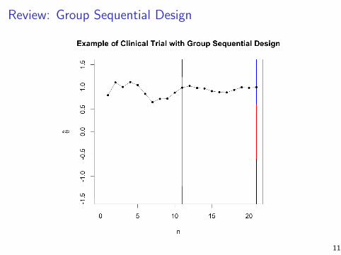
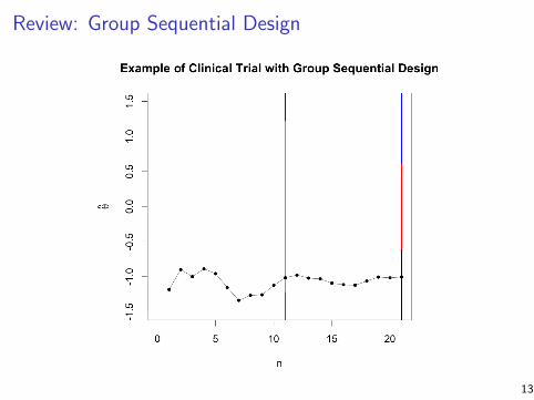
Review: Group Sequential Design

8

Review: Group Sequential Design

9

Review: Group Sequential Design

10

Review: Group Sequential Design

11

Review: Group Sequential Design

12

Review: Group Sequential Design

13

Review: Group Sequential Design

14

Review: Adaptive Design

15

Review: Adaptive Design

16

Review: Adaptive Design

17

Review: Adaptive Design

18

Review: Inference when using GS or Adaptive Designs

I Neyman-Pearson lemma, Karlin-Rubin theorem not applicableI Likelihood ratio not monotone non-decreasing when using

group-sequential-like designs

I Need some way (some ordering) to determine what are“extreme” observations under the null hypothesis

19

Review: Considered Orderings

I Sample meanI Signed LR: If ∀ fixed θ∗,

sign(θ̂(1) − θ∗

) f(outcome 1|θ = θ̂(1)

)f (outcome 1|θ = θ∗)

> sign(θ̂(2) − θ∗

) f(outcome 2|θ = θ̂(2)

)f (outcome 2|θ = θ∗)

,

then outcome 1 ordered higher than outcome 2, with θ̂(i) thesample mean from outcome i

I Conditional Error Ordering: Outcomes ordered according tothe stage-wise p-value of “backward image”

20

Review: Point Estimates

Three point estimates considered

I Sample mean (MLE) θ̂

I Bias adjusted mean (BAM) η̂: the value θ for which θ̂ is themean

I Median-unbiased estimate (MUE) ζ̂: the value θ for which θ̂is the median

21

Distribution of Sampling DensityLaw of Total Probability:

Fθ̂|θ(x) = Pθ

(θ̂ ≤ x

)=∑n

i=0Pθ

(θ̂ ≤ x |Ci

)Pθ(Ci )

=∑n

i=0Fθ̂|θ,Ci (x)Pθ(Ci ).

Taking derivatives:

fθ̂|θ(x) =d

dxFθ̂|θ(x)

=d

dx

∑n

i=0Fθ̂|θ,Ci (x)Pθ(Ci )

=∑n

i=0

d

dxFθ̂|θ,Ci (x)Pθ(Ci )

=∑n

i=0fθ̂|θ,Ci (x)Pθ(Ci ).

22

Distribution of Sampling Density

C0: the stopping region.

Fθ̂|θ,C0(x) = Pθ

(θ̂ ≤ x |C0

)= Pθ

(θ̂ ≤ x |θ̂1 /∈ (a1, d1)

)=

Pθ

(θ̂ ≤ x , θ̂1 /∈ (a1, d1)

)Pθ

(θ̂1 /∈ (a1, d1)

)=

Fθ̂1|θ(x)× 1{θ̂1 /∈(a1,d1)}Pθ

(θ̂1 /∈ (a1, d1)

)

23

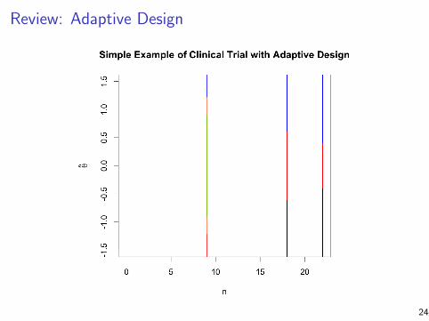
Review: Adaptive Design

24

Distribution of Sampling Density

Taking derivatives once more:

fθ̂|θ,C0(x) =d

dxFθ̂|θ,C0(x)

=fθ̂1|θ(x)× 1{θ̂1 /∈(a1,d1)}Pθ

(θ̂1 /∈ (a1, d1)

) .

25

Distribution of Sampling Density

Ci , i ≥ 1: a continuation region.

I m = sample size at interim analysis

I N = m + n = sample size at final analysis

I θ̂ = mN × θ̂1 + n

N × θ̂2

26

Distribution of Sampling Density

Ci , i ≥ 1: a continuation region.

Fθ̂|θ̂1=x(z) = Pθ

(θ̂ ≤ z |θ̂1 = x

)= Pθ

(mN× θ̂1 +

n

N× θ̂2 ≤ z |θ̂1 = x

)= (some algebra)

= Fθ̂2|θ

(N

n

(z − mx

N

))Derivative:

fθ̂|θ̂1=x(z) = fθ̂2|θ

(N

n

(z − mx

N

))N

n

27

Distribution of Sampling Density

Ci , i ≥ 1: a continuation region. Convolution:

fθ̂|Ci (z) =

∫ ∞−∞

fθ̂|θ̂1(z)fθ̂1(x)dx

I R can compute this numerically.

28

Simulation Results

Settings:

I Recalling that θ := µtreat − µplac , interested in testingH0 : θ ≤ 0 vs. H1 : θ > 0

I Assumed: σ2 = 0.5

I Desired: Level α = 0.025 at θ = 0, power of 0.9 at θ = 1

I Continuation region from original GS design divided into 10equally sized continuation regions

I Adaptive rule: Final sample sizeN∗(t) = 2.02N − 1.627 (t − 1.96), with t the midpoint of thenew continuation region.

I Standard boundaries derived similarly to those in GS design

29

Simulation Results

Procedure:I Through grid search, get boundaries and sample sizes needed

to achieve desired size and powerI Computationally demanding

I Run clinical trial (or simulate data)I Computationally easy

I Draw inference from observed dataI Computationally intense

30

Simulation ResultsScenario 1: Distribution assumptions hold

31

Simulation ResultsScenario 1: Distribution assumptions hold

32

Concern

Distribution Assumptions

I Known variance

I Normality

33

Simulation ResultsScenario 2: Normality holds, but true σ2 = 1

34

Simulation ResultsScenario 2: Normality holds, but true σ2 = 1

35

Simulation ResultsScenario 3: Data exponentially distributed, appropriately scaledand shifted so that σ2 = 0.5 and θ ∈ (0, 2)

36

Simulation ResultsScenario 3: Data exponentially distributed, appropriately scaledand shifted so that σ2 = 0.5

37

Additional Concern

Knowledge of the final sample size is potentially unblinding.I Same could be said of group sequential design, but group

sequential design is widely acceptedI Not a great answer, but it’s something

I No clear way to quantify effects of such an unblinding

38

Summary

I Whether or not adaptive designs are a good idea, they areimplemented to find cures for things such as [insert type ofcancer here], so their properties need to be understood

I Under sample mean ordering and either type of boundarydesign, all 3 estimators do reasonably well, and confidenceintervals do okay when θ is close to 0

I Inference not necessarily robust to violations of distributionassumptions

39

Questions?

40