An Equilibrium Model of Asset Pricing and Moral Hazard

Hui Ou-Yang∗

Fuqua School of BusinessDuke University

Durham, NC 27708-0120huiou@duke.edu(919) 660-3790

This Version: June 1, 2002

∗This paper represents a major extension of a section in Chapter 2 of my Ph.D. dissertation submitted to theUniversity of California at Berkeley, where a two-asset equilibrium was developed. I am very grateful to Navneet Arorafor his contribution in a partial solution to the first best case presented in Lemma 3 of the paper. I also thank TomAhn, Moshe Bareket, Michael Brennan, Peter DeMarzo, Cam Harvey, Hua He, Rich Kihlstrom, Pete Kyle, HayneLeland, Jun Liu, Michael Roberts, Mark Rubinstein, Matt Spiegel, S. Viswanathan, Jonathan Wang, Wei Xiong, andseminar participants at Caltech, Duke, Princeton, UCLA, UNC, and Wharton for their comments.

Abstract

This paper develops an integrated model of asset pricing and moral hazard. In particular,

we combine a version of the Capital Asset Pricing Model (CAPM) with a multi-agent moral

hazard model. The excess dollar returns for risky stocks, optimal contracts for managers

(agents) that involve relative performance, and equilibrium stock prices are explicitly charac-

terized. We show that the CAPM linear relation in terms of the expected dollar returns still

holds in the presence of moral hazard and that our β is given by the ratio of the covariance

between a firm’s stock return and the market return over the variance of the market return,

with both returns adjusted for the compensation to the managers. The equilibrium price of a

stock decreases with its idiosyncratic risk, but the expected excess dollar return of the stock is

independent of it. Consequently, the risk premium, which is defined as the ratio of the excess

return to the stock price, increases with idiosyncratic risk. We also show that the risk aversion

of the principal in our model leads to less emphasis on relative performance evaluation than

in a model with a risk-neutral principal. This result may shed light on why the empirical

evidence for relative performance evaluation is mixed, even though the theoretical prediction

based on a risk-neutral principal strongly supports it. In addition, we show that if the manager

of a firm is compensated based solely on his own performance, then the expected dollar return

of the firm increases with its idiosyncratic risk. This exercise illustrates that, in the presence

of moral hazard, contracting plays a key role in the determination of the expected return of

a stock. Furthermore, we show that under certain conditions, the equilibrium contract is a

linear combination of the stock price and the level of the market portfolio.

1

1 Introduction

In many equilibrium asset pricing models, the dividend or cash flow processes are specified

exogenously by either normal or lognormal processes. For example, the Capital Asset Pricing

Model (CAPM) of Sharpe (1964), Lintner (1965), and Mossin (1966) shows that the excess

return of a stock is linearly related to the excess return of the market portfolio. The slope

coefficient in this relation, β, is defined by the ratio of the covariance between the asset and

market returns to the variance of the market return.1 Thus, idiosyncratic or firm-specific risk

plays no role in the determination of the expected return of an asset.

In reality, however, a firm’s cash flows are owned by its investors or shareholders, but

influenced by its manager who cannot fully hedge against the firm’s idiosyncratic risk. Since

the interests of the manager (the agent) and the shareholders (the principal) may not be

perfectly aligned, there exists a potential moral hazard problem. This conflict raises two key

questions. First, does the linear relation between the expected excess return of an asset and

the expected excess return of the market still hold? And, second, does idiosyncratic risk affect

the expected return of an asset in the presence of moral hazard?

On the other hand, many principal-agent models solve for optimal contracts or risk sharing

rules in the absence of financial markets. Intuitively, a principal hires an agent to manage

a project and designs a contract so as to induce the agent to exert appropriate effort. Gen-

erally, the principal is precluded from investing in the financial market. For example, in the

multi-agent moral hazard model of Holmstrom (1982), a risk-neutral principal hires multiple

risk-averse agents in a one-period economy. The value of each project is composed of a fixed

component under the control of an agent, and a random component representing unforesee-

able events. Among several fundamental contributions to the literature, Holmstrom discusses

relative performance evaluation (RPE) and finds that the RPE improves welfare under two

conditions: if the outputs across projects are correlated with one another, and if the RPE is

used to filter out the systematic or common risk from the agents’ compensation. Baiman and

Demski (1980) and Diamond and Verrecchia (1982) obtain similar results in more specialized

settings. It would be of interest to determine whether these results are robust with respect to

risk-averse principals in an equilibrium asset pricing framework.

Early developments on the valuation of assets under moral hazard include the one-period

1See Ross (1976) for the Arbitrage Pricing Theory. See, e.g., Merton (1973), Rubinstein (1976), Lucus (1978), andBreeden (1979) for multi-period asset pricing models. See, e.g., Roll (1977) for a critique of empirical tests of theCAPM.

2

models of Diamond and Verrecchia (1982) and of Ramakrishnan and Thakor (1982,1984).

Diamond and Verrecchia derive an optimal managerial contract in an equilibrium model in

which identical risk-neutral investors trade between a riskless bond and a risky stock. They

show that systematic risk is completely removed from the manager’s compensation scheme.

Since this model has only one risky asset, the role of idiosyncratic risk in asset returns cannot

be rigorously addressed and a CAPM-type relation may not be obtained. Ramakrishnan and

Thakor (1984) extend the Diamond-Verrecchia model to incorporate a risk-averse investor as

well as the commonly used normal distribution for asset returns.2 They show that in the

absence of moral hazard, managers are insured against idiosyncratic risks, but when moral

hazard is included, contracts depend on both systematic and idiosyncratic risks. Ramakrish-

nan and Thakor demonstrate their results in a partial equilibrium model which assumes that

contracts are linear, that the Arbitrage Pricing Theory holds with moral hazard, and that the

return on an asset increases with the agent’s effort level.

The objective of this paper is to develop an integrated model of asset pricing and moral

hazard.3 In particular, we develop a version of the CAPM in the presence of moral hazard as

well as a multi-agent moral hazard model by allowing principals to be risk averse and to trade

in the financial market. In doing so, we combine a model of the security market with that

of an optimal contract. Following Holmstrom and Milgrom (1987), we adopt a continuous-

time framework for its convenience in the derivation of optimal contracts. Our model may be

viewed as an extension of Holmstrom and Milgrom in the presence of both multiple agents

and a principal who can trade in a securities market, as well as an extension of Diamond

and Verrecchia (1982) in the presence of risk-averse investors and multiple risky assets. Our

model shall also generalize the Ramakrishnan-Thakor model by deriving rather than assuming

an asset pricing model in the presence of moral hazard, and by assuming that the cash flow

process of an asset rather than the return process on the asset increases with the agent’s

effort level. Since the linear contract is typically not optimal in a one-period principal-agent

model,4 we deduce optimal contracts from a larger contract space. We explicitly characterize

equilibrium asset prices, expected asset returns, and optimal contracts in a large economy. It

is essential to have closed-form solutions in order to determine whether the CAPM relation2In Diamond and Virrecchia, the uniform distribution for the systematic risk factor and the exponential distribution

for the other part of the output are adopted for tractability in the derivation of optimal contracts.3See, e.g., Brennan (1993), Allen (2001), and Arora and Ou-Yang (2001) for integrated models of asset pricing and

delegated portfolio management, which may also involve moral hazard problems.4See, e.g., Mirrlees (1974) for details.

3

holds and to understand how both the risk aversion of a principal and the risk exposure of an

asset affect relative performance evaluation.

We find that the expected excess dollar return (as opposed to the rate of return) of a

stock less the expected compensation to the manager is linearly related to the return on the

market portfolio. Similarly, the slope of the relation is the CAPM β adjusted for risk sharing.

Specifically, our β is given by the ratio of the covariance between a firm’s stock return and the

market return to the variance of the market return, with both the stock return and the market

return adjusted for the compensation to the managers. The expected dollar return of a stock

is found to be independent of its idiosyncratic risk. This result clarifies both the intuition

of Holmstrom (1982) and the calculation of Diamond and Verrecchia (1982). In the absence

of an equilibrium asset pricing model, Holmstrom cannot identify separately the individual

impact of idiosyncratic risk on the return and price. Diamond and Virrecchia conclude that

a risk-neutral investor can earn a higher dollar profit by adopting a project with a lower

idiosyncratic risk. Their calculation assumes that investors are concerned with the expected

value of the output at the end of the period net the expected value of the payment to the

manager, ignoring the current stock price or the initial cost to acquire the stock. Furthermore,

any partial equilibrium model in the absence of equilibrium prices would lead to the conclusion

that investors demand a higher expected dollar return for an asset with a higher idiosyncratic

risk.

The firm-specific risk, however, does affect equilibrium stock prices.5 The higher the

firm-specific risk, the higher the investors’ marginal cost of providing incentives to the risk-

averse manager, and thus the stock price is lower in equilibrium. Intuitively, when the firm-

specific risk is higher, investors must compensate the manager more on a risk-adjusted basis,

and consequently, they pay a lower price for the stock in equilibrium. The net result is

that the expected dollar return adjusted for the manager’s compensation remains the same,

independent of the firm-specific risk. If we define the risk premium of a stock as the ratio of

its expected excess return to the current stock price, then the risk premium increases with

the firm-specific risk.

As in the Baiman-Demski (1980), Diamond-Verrecchia (1982), and Holmstrom (1982) mod-

els, when investors are risk neutral, the use of RPE completely filters out the systematic risk

from the manager’s compensation in our equilibrium model. With risk-averse investors, our

5In the absence of moral hazard, idiosyncratic risk does not affect asset prices. See, e.g., Ross (1976), Ingersoll(1987), and Cochrane (2001) for discussions.

4

optimal contracts show that, in equilibrium, investors and managers share the systematic risk

optimally, as if there were no moral hazard, and the incentive part of the contract involves

only the firm-specific risk.6 In other words, the firm-specific risk and systematic risk are com-

pletely separate from each other in the manager’s compensation. Due to the separation of

these two types of risks, the firm-specific risk does not affect the expected dollar return, which

depends on the covariance between the individual stock and the market portfolio.

The RPE with respect to the market portfolio has been the focus of extensive empirical

testing,7 but the evidence has been mixed.8 Murphy (1999) notes that the scope for RPE in

actual explicit contracts is limited: just over 20% of the 125 surveyed industrial companies use

some form of RPE in annual bonus plans.9 The empirical studies of RPE have focused mainly

on the implicit relation between CEO compensation, firm performance, and market and/or

industry performance. For example, Antle and Smith (1986), Barro and Barro (1990), Jensen

and Murphy (1990), Janakiraman, Lambert, and Larcker (1992), Aggarwal and Samwick

(1999a), and Bertrand and Mullainathan (1999) find little evidence of RPE. Aggarwal and

Samwick (1999b) even find positive RPE in some cases. On the other hand, Gibbons and

Murphy (1990), Sloan (1993), and Himmelberg and Hubbard (2000) find empirical support

for RPE. Summarizing the empirical findings, Abowd and Kaplan (1999) and Prendergast

(1999) have identified the lack of widespread use of RPE in executive compensations as an

unresolved puzzle.

We show that the optimal sharing of systematic risk between risk-averse investors and

risk-averse managers reduces the magnitude of RPE. On the one hand, since the systematic

risk can be inferred by investors in a large economy, investors would like to reduce the risk-

averse manager’s exposure to this risk by the use of RPE (a negative coefficient in front of

the market portfolio in the manager’s compensation). On the other hand, unlike risk-neutral

investors who can bear all of the systematic risk, risk-averse investors must share it with

risk-averse managers, which results in a positive coefficient in front of the market portfolio.

Consequently, the RPE in this case is smaller than the value obtained in previous models in

which the principal is risk neutral. Specifically, we show that the RPE is determined by both

6Mathematically, the manager’s effort term, which is a function of the firm-specific risk, does not interact with thesystematic risk term.

7For example, if the stock of a firm is positively correlated with the market portfolio, then its executive compensationshould be negatively related to the performance of the market portfolio.

8For comprehensive reviews, see, e.g., Abowd and Kaplan (1999), Murphy (1999), Prendergast (1999), and Core,Guay, and Larcker (2001).

9See Table 9 of Murphy (1999).

5

the risk aversion of the investors and the ratio of the standard deviation of the firm’s cash

flow to that of the market portfolio. For example, the RPE can even be positive if the ratio

of the two standard deviations is small enough. Furthermore, we show that under certain

conditions, the optimal contract is a linear combination of the stock price and the level of the

market portfolio.

Since RPE is not widely adopted in executive compensation, we examine the impact of

moral hazard on asset returns in the absence of RPE. In this case, we assume that managers

are compensated based solely on their own performance. Due to the suboptimal sharing of

systematic risk in this smaller contract space, we find that the expected dollar return of a stock

increases, its stock price decreases, with the level of idiosyncratic risk. When idiosyncratic

risk increases, both the risk-averse manager’s effort level and the fraction of the firm shared

by the manager decrease in equilibrium. As a result, the risk-averse investors must bear more

of the systematic risk in equilibrium,10 and therefore, they demand a higher dollar return

for the stock. This exercise illustrates that in the presence of agency problems, optimal

contracting plays a key role in the determination of asset returns and that in the absence

of RPE, idiosyncratic risk still matters to asset returns even though investors may be fully

diversified.

Empirically, Campbell, Lettau, Malkiel, and Xu (2001) find that there has been a notice-

able increase in firm-level volatility relative to market volatility, and Malkiel and Xu (2000)

and Goyal and Santa-Clara (2001) demonstrate that idiosyncratic risk contributes to expected

asset returns. Our theoretical model provides a potential mechanism for incorporating idiosyn-

cratic risk into asset returns, and may help explain the findings of Malkiel and Xu and Goyal

and Santa-Clara.

The rest of the paper is organized as follows. The next subsection briefly reviews more

related theoretical literature. Section 2 describes the model. As a benchmark case, Section

3 reviews the CAPM linear relation in the absence of moral hazard. The expressions for

expected returns, equilibrium stock prices, and optimal contracts in the presence of moral

hazard are derived in Section 4. Some concluding remarks are offered in Section 5. All proofs

are given in the appendix.

10The output of a firm is partially driven by the systematic risk. If the manager shares a smaller portion of the firm,then he bears less systematic risk. Consequently, investors must bear more systematic risk.

6

1.1 More Related Literature

The Holmstrom-Milgrom (1987) model provides insights into the solution of optimal contracts

in our model.11 In this model, both the principal and the agent have exponential utility

functions. The output process is given by a Brownian motion plus a drift term. The principal

is passive and the agent continuously controls the drift rate of the output process. It is shown

that the optimal contract is a linear function of the terminal value of the output process.

Some recent work investigates the impact of moral hazard on the market risk premium

demanded by a representative agent who manages a single firm. Kahn (1990) develops a two-

period model in which the agent has a power utility function and the output follows a binomial

distribution. Numerical results demonstrate a larger equity premium than in the standard

representative agent model. Kocherlakota (1998) points out that the higher equity premium

may be due to a restriction in Kahn’s model which prevents the agent from diversifying his

wealth. Kocherlakota extends Kahn’s model to allow a representative agent to diversify across

assets; namely, the agent can sell a fraction of his own firm and buy a fully diversified mutual

fund. All the trades by the agent are assumed to be public information. Numerical calculations

generate a smaller equity premium.

Another line of research examines the efficiency of equilibrium allocations and the agent’s

trading strategies. In the models of Kihlstrom and Matthews (1990) and Magill and Quinzii

(2000),12 an agent initially owns the entire firm. His costly, unobservable effort affects the

mean of the output. The agent sells a fraction of the firm to outside investors for risk sharing

and other purposes. How much equity he retains determines his incentives and is assumed

to be observed by outside investors. In equilibrium, the agent may not want to sell the

entire firm, because outside investors will then infer that the agent will not exert any effort,

thus lowering the equity price. This idea is related to the signaling equilibria in Leland

and Pyle (1977). DeMarzo and Urosevic (2001) solve a multi-period model for the optimal

trading strategy of a large agent-shareholder who undertakes costly effort to improve a firm’s

dividends. This shareholder faces a tradeoff in which selling shares will likely lower the share

price, while retaining them results in a less diversified portfolio. Among other contributions,

they demonstrate that their model can help to explain both IPO underpricing and the use

of lockup provisions. Urosevic (2001) extends the DeMarzo-Urosevic model to incorporate

11See also Schattler and Sung (1993) and Ou-Yang (2000).12Magill and Quinzii extend the Kihlstrom-Mattews model to include multiple assets and a more general capital

structure.

7

multiple risky assets with a single agent. Whenever feasible, the agent will trade in other

assets in order to hedge part of the systematic risk. In doing so, the agent will sell off the

firm under his control more slowly. On the other hand, if the agent cannot trade in other

assets, then he will sell his own firm more rapidly. Since there is only one effort-exerting agent

and since systematic and idiosyncratic risks are not precisely specified, one cannot obtain a

CAPM-type equation that relates a firm’s return to the market return. Consequently, this

model is not designed to address the impact of risks on asset returns and the role of risks in

the determination of RPE.

Finally, Merton (1971), Duffie et al. (1997), Heaton and Lucas (2000), and Liu (2001),

among others, study the impact of idiosyncratic risk on portfolio choice in partial equilib-

rium settings. Admati (1985), Diamond and Verrecchia (1991), Wang (1993), and Easley and

O’Hara (2001), among others, examine the role of information risk in determining asset re-

turns. Stulz (1999) presents arguments for why total risk might matter. Storesletten, Telmer,

and Yaron (2001) and Dai (2002) demonstrate that idiosyncratic risk in labor income helps

determine asset returns.

In summary, since the closed-form expressions for both the expected returns on assets

and the optimal contracts for agents have not been obtained in a large economy, the existing

literature cannot adequately address the impact of idiosyncratic risk on expected returns as

well as the issue of relative performance in the presence of risk-averse principals.

2 The Model

For the tractability of derivation of optimal contracts, we consider a continuous-time economy

on the finite time horizon [0, T ]. The following assumptions characterize our economy.

Assumption 1: There is one riskless asset and N risky assets available for continuous

trading. The cumulative dividend or cash flow process of firm i is given by

dDit = (Ait + ΠiDit)dt + σicdBct + σiidBit

≡ (Ait + ΠiDit)dt + biDdBt, i = 1, 2, · · · , N, (1)

with the initial condition that Di0 = di0. Here, the transpose of Bt is defined as

BTt = (Bct, B1t, B2t, · · · , BNt), representing a (1 × (N + 1)) vector of independent standard

Brownian motion processes, biD is defined as biD = (σic, · · · , σii, · · · , 0), which is a (1×(N +1))

vector of constants, with the first and the ith element being non-zero. Thus, the cash flow

8

processes across assets are correlated through the common Brownian motion Bct. Ait denotes

the effort or action taken by the manager of the ith firm. The manager influences the cash

flow process through his effort Ait in the drift term. For tractability, we follow Holmstrom and

Milgrom (1987) in assuming that the manager’s action does not influence the diffusion rate of

the cash flow process. Since we shall solve for optimal efforts A∗t in closed form, in equilibrium,

it shall become clear that the above Dt processes are well-defined semimartingales and that

there exist unique solutions to them.

The riskless asset yields a positive constant rate of return r.

Assumption 2: The manager of firm i incurs a cumulative cost of∫ T0 ci(t)dt associated

with managing the firm from time 0 to T . The cost rate is given by a convex function:

ci(t) =1

2ki(t)A

2it,

where ki(t) is a deterministic function of time t and the marginal cost rate increases with the

level of effort, which helps guarantee a solution to the manager’s maximization problem. At

time T , manager i receives a salary of SiT , from the investors or principals.13 Managers expend

efforts for their respective firms and are barred from trading securities for their own accounts.

In other words, the only source of income for the managers is from the compensation paid by

the investors.

It would be essential to assume that managers cannot short their own stocks. Otherwise,

they can undo the incentives completely. In practice, executives are not allowed to short

their own stocks. If we assume, as in Kihlstrom and Matthews (1990), Kocherlakota (1998),

Magill and Quinzii (2000), DeMarzo and Urosevic (2001), and Urosevic (2001), that managers’

trades are observable to investors, then this assumption can be enforced by a clause in the

contract. In other words, investors can solve the trading strategies for managers and enforce

them through contracting. It shall be seen that even though managers cannot diversify on

their own, the optimal compensation schemes provide each manager with a holding of his own

firm for incentive purposes and a fully diversified market portfolio for risk sharing purposes.14

Assumption 3: The N firms are run by N managers, each of whom has a negative

exponential utility function with a risk aversion coefficient Ra.15 The exponential utility

13We shall use agent and manager, and principal and investor interchangeably.14It means that our results would remain the same even if the manager is allowed to invest privately in the market

portfolio.15The manager of each firm may be interpreted as a representative of the management team including all top

executives of the firm.

9

functions are assumed for tractability of the derivation of optimal contracts. Notice that the

N managers are not the same due to different ki(t)’s in the cost functions. It is not essential

to assume the same risk-aversion coefficient for managers.

Given the investor’s contract SiT , the manager expends efforts so as to maximize his own

expected utility:

sup{Ait}

E

[− 1

Ra

exp

[−Ra

(Si

T −∫ T

0ci(t)dt

)]],

subject to the cash flow processes. Following Holmstrom and Milgrom (1987), we assume that

there are no intertemporal consumptions by either investors or managers and that managers

receive their compensation at the terminal date only.16 Accordingly, we assume that there are

no intertemporal dividend payments. At the terminal date, investors receive dividends and

simultaneously compensate their managers based on the amount of dividends generated.

Assumption 4: As in Diamond and Verrecchia (1982), there are N identical investors in

our economy.17 All investors have a negative exponential utility function with a risk aversion

coefficient Rp. Each investor decides on the number of shares to invest in the riskless bond and

the risky stocks, and designs incentive contracts for managers so as to maximize the expected

utility over her terminal wealth:

sup{µt,At},Si

T

E

[− 1

Rp

exp

[−Rp

(WT −

N∑i=1

SiT ({µt})

)]],

subject to her wealth process {Wt} and managers’ participation and incentive compatibility

constraints.

The investor’s wealth process Wt shall be given in later sections where we solve for the

investor’s and the managers’ maximization problems. A manager’s participation constraint af-

fords the manager a minimum utility level that the manager would otherwise achieve elsewhere

in the labor market.18 His incentive compatibility constraint means that the investor’s compen-

sation scheme and action must satisfy the manager’s maximization problem, i.e., the investor’s

optimal actions At must coincide with those of the managers in equilibrium. Otherwise, the

16In the Holmstrom-Milgrom model, if the agent’s compensation takes place continuously, then it can be seen thatthe optimal contract is still linear.

17This assumption is for tractability. Since investors can invest in every stock in the economy, if they are different,they may want to induce different effort levels for the manager of the same firm. It is much easier to solve for asymmetric equilibrium in which investors’ solutions are identical.

18We here assume that the investor has all the bargaining power. It is easy to show that as long as both the managerand the investor have exponential utility functions, the equilibrium effort and optimal contract form remain the same,even if the manager has the bargaining power. The only difference is in a constant term in the optimal contract, whichensures that the investor rather than the manager achieves his reservation wage.

10

manager would not adopt the action desired by the investor. Here At = (A1t, A2t, · · · , ANt),

µ = (µ1j, µ2j, · · · , µNj), where µij denotes the number of shares for firm i demanded by in-

vestor j, and SiT ({µt}) represents the investor’s share of payment to the manager for holding

{µt} shares of the firm. In other words, an investor’s payment to a manager depends on her

ownership of the firm. This point shall be made more precise in Assumption 7 to be specified

in subsection 4.2.

Each firm has one share available for trading, and there is an unlimited supply of the

bond. µij then denotes the fraction of firm i owned by investor j. As in Lucas (1978), since

the market must clear at all times, in equilibrium, the N identical investors will hold all the

firms in the economy completely, i.e., µij = 1/N , or∑N

j=1 µij = 1, i = 1, 2, · · · , N .

Assumption 5: Following the traditional asset pricing literature where exponential utility

functions and normal dividend processes are employed,19 we assume that the equilibrium

pricing function is of the following linear form:

Pit = λi0(t) +N∑

j=1

λij(t)Djt, (2)

where the coefficients λ’s are time-dependent deterministic functions. We shall specify the

boundary conditions in later sections.

For ease of exposition, we express the price vector in a compact form as

dPt = aP dt + bP dBt, (3)

where aP is a (1×N) column vector with the ith element given by

aPi= λi0 +

N∑j=1

[λijAjt +

(λij + Πj

)Djt

],

and where bP represents an (N × (N + 1)) matrix with the ith row given by

bPi=

N∑j=1

λijbjD.

Recall that bjD is a row vector with (N + 1) elements.

Assumption 6: The contract space is given by

SiT = E i

T (T, DT , PT ) +∫ T

0αi(t,Dt, Pt)dt +

∫ T

0βi(t,Dt, Pt)dPt, (4)

19See, e.g., Campbell and Kyle (1993), Wang (1993), and He and Wang (1995).

11

where ET is a general function of T , DT , PT , and where α and β are unknown coefficients

that depend upon t, Dt, and Pt.20 Note that βi and P denote a row and a column vector,

respectively. Within our linear pricing function, Dt and Pt are interchangeable in the contract

form. Though the pricing function is constrained to be linear, this contract space covers linear,

nonlinear, path-independent, and certain path-dependent functions.

3 The Benchmark Case: A Pure Exchange Economy in the Ab-sence of Managers

Let us first consider a benchmark case in which the Ait’s in the dividend processes are exoge-

nously given or in which there are no managers. The equilibrium stock prices and returns are

completely determined by both the dividend processes and the investors’ demand for risky

assets.

From the linear pricing function, the boundary conditions are given by λi0(T ) = 0, λii(T ) =

1, and λij = 0 when i 6= j. The excess dollar return for holding stock i within time interval

dt is defined as21

dQi = dPit − rPitdt.

Substituting the conjectured form for Pit into the above expression, we get

dQi =

λi0 − rλi0 +N∑

j=1

λijAjt +N∑

j=1

(λij − (r − Πj) λij

)Djt

dt +N∑

j=1

λijbjDdBt.

For simplicity, we write

ai0 = λi0 − rλi0 +N∑

j=1

λijAjt; aij = λij − (r − Πj) λij.

The excess return then takes the following form:

dQi =

ai0 +N∑

j=1

aijDjt

dt +N∑

j=1

λijbjDdBt ≡ aiQdt + bi

QdBt.

For convenience, we shall denote by dQ the (1×N) column vector of excess returns composed

20This contract space is adapted from Schattler and Sung (1993) and Ou-Yang (2000). We further assume that thecoefficients satisfy the regularity conditions similar to those given in Ou-Yang.

21The dDt term does not appear in the excess return process because of the assumption that there are no intertemporaldividend payments.

12

of dQi and write dQ ≡ aQdt + bQdBt. By definition, we have

aQ =

a1Q

a2Q

···

aNQ

, bQ =

b1Q

b2Q

···

bNQ

.

It is well known that investor i’s wealth process is given by22

dWit = rWitdt + µidQ,

where µi denotes a row vector defined as µi = [µ1i, µ2i, · · · , µNi]. For simplicity, we shall omit

the subscript i in the expressions for µi and Wit. The investor’s problem is to maximize her

expected utility over the terminal wealth:

supµ

E

[− 1

Rp

exp (−RpWT )

]s.t. dWt = rWtdt + µdQ.

For comparison with the moral hazard case to be solved later, we present a CAPM-type

equation for the excess return on the stock in the following lemma.

Lemma 1. In equilibrium, the expected excess dollar return aiQ on stock i is a linear

function of the expected excess dollar return aMQ on the market portfolio:

aiQ =

Cov(dPi, dPM)

V ar(dPM)aM

Q ,

where the market portfolio is defined as PM = µMP = P1 + P2 + · · ·PN .23 This is the CAPM

relation in terms of the excess dollar return. The expected excess rates of returns on stock i

and the market portfolio, RiQ = 1

Piai

Q and RMQ = 1

PMaM

Q , also satisfy the CAPM equation:

RiQ =

Cov(Ri, RM)

V ar(RM)RM

Q ≡ βRMQ .

22See, e.g., Wang (1993) and Duffie (2001) for references.23See also Lo and Wang (2001) and others for the same definition of the market portfolio. This definition of the

market portfolio is perhaps more appropriate for the discussion of the dollar returns in a normal-exponential modellike ours. The value-weighted market portfolio is mainly adapted for the discussion of the rates of return.

13

4 A Principal-Agent Economy

We now consider the case in which the drift rate of each dividend process is controlled by a

manager at a cost. The investor must provide the manager with the right incentives for him

to exert appropriate effort. In doing so, we extend the current asset pricing literature by par-

tially endogenizing the dividend process. To solve for an equilibrium, we must determine the

equilibrium pricing functions and the optimal contracts simultaneously under the conditions

that markets clear and that managers adopt optimal controls for both themselves and the

investors.

4.1 An Expression for the Optimal Fee Structure

In this subsection, we provide an expression for the optimal fee structure to be denoted by

SiT in terms of the manager’s value function and the coefficient vectors in the contract form,

β, using the manager’s participation constraint. This optimal fee equals the optimal contract

at the optimal action A∗it. Si

T , however, may not implement investors’ optimal action.24

Since SiT satisfies the manager’s participation constraint, it greatly simplifies the investors’

dynamic maximization problem. Investors use SiT to first solve for both optimal actions and

the coefficients in the original contract space and then construct optimal contracts in terms

of the variables such as stock prices that are observed by both investors and managers.

Given the contract space SiT in Eq. (4), we define a value function process V i(t, Pt) for

manager i’s maximization problem as25

V i(t, P ) = sup{Aiu}

Et

[− 1

Ra

exp

{−Ra

[EiT +

∫ T

t[αi(u, Pu)− ci(u, Aiu)]du +

∫ T

tβidPu

]}].

Ou-Yang (2000) has shown that under a regularity condition, the following Bellman type

equation is both a necessary and a sufficient condition for the manager’s dynamic maximization

problem:

0 = supAit

[−RaVi(t, P ){αi(t, P ) + βi(t, P )aP − ci(t, Ai)−

1

2Raβi(t, P )bP bT

P βT (t, P )}

+V it + V i

P [aP −RabP bTP βT

i (t, P )] +1

2tr(V i

PP bP bTP )]. (5)

Here, the subscripts denote the relevant partial derivatives of V i(t, P ).

24See Ou-Yang (2000) for details.25For notational convenience, we shall write P and D rather than Pt and Dt in the expressions that follow.

14

Using the manager’s participation constraint at time 0, the above PDE, Ito’s lemma, and

a transformation, we can arrive at an expression for the equilibrium fee SiT , which is presented

in the next lemma.

Lemma 2. The equilibrium fee is given by

SiT = Ei0 +

∫ T

0ci(t)dt +

Ra

2

∫ T

0βibP bT

P βTi dt +

∫ T

0βibP dBt, (6)

where Ei0 denotes manager i’s certainty equivalent wealth at time 0, and where ci(t) = 12ki(t)A

2it

and βi = βi −V T

P

RaV.

Remark 1. This equilibrium fee has an intuitive interpretation. At the terminal date,

investors pay the manager his reservation wage, reimburse the manager’s operating costs,

compensate the manager in the third term for the risk that he bears in the fourth term, and

the fourth term involves Brownian motion processes and represents the risk in the manager’s

compensation scheme. Note that if the manager is risk neutral, then the third term vanishes,

because a risk-neutral manager does not require compensation for bearing risk.

Remark 2. Substituting this equilibrium fee into the manager’s participation constraint

and assuming that the Novikov condition holds,26 we obtain

E0

[− 1

Ra

exp

{−Ra

[Ei0 +

Ra

2

∫ T

0βibP bT

P βTi dt +

∫ T

0βibP dBt

]}]= − 1

Ra

exp(−RaEi0).

Therefore, the manager’s participation constraint is satisfied, which eliminates the α coefficient

from the expression for SiT . On the other hand, if the manager has the bargaining power, we

can always adjust the constant term Ei0 so that the investor achieves her reservation utility,

and the risk sharing part of the contract would remain intact. Consequently, the optimal effort

would be the same, which must satisfy both the investor’s and the manager’s maximization

problems.

Using the above equilibrium fee, the investors can simply ignore the manager’s participation

constraint when solving their maximization problems to determine the optimal effort level and

trading strategies. We next solve for the optimal contracts, equilibrium prices, and expected

excess returns in the first and second best cases. In the first best case, since the manager’s effort

is observed by the investor, we can ignore the manager’s maximization problem and simply

solve the investor’s maximization problem using the above equilibrium fee. In the second best

26See, e.g., Karatzas and Shreve (1991) and Duffie (2001). It shall be shown that all components in vector βi in ourequilibrium solutions are bounded, deterministic functions, the Novikov condition is thus satisfied.

15

case, we must take the first-order condition of the manager’s Bellman equation into account.

It must also be verified that the manager’s Bellman equation is satisfied. Furthermore, It

shall be seen that as in the Holmstrom-Milgrom model, since all the optimal solutions are

bounded, deterministic functions, the manager’s Bellman equation will be sufficient for his

maximization problem.

4.2 The Valuation Relation in the First Best Case

Notice that this case generally differs from the benchmark case discussed in the previous

section where there are no managers in the economy. In the current situation, the investors

must still share the risks associated with the cash flows with the managers, even though there

are no agency problems involved. Recall that an investor’s holdings (number of shares invested

in the risky assets) are defined as µ =[

µ1 µ2 · · · µN

]. Since all investors are identical, we

have ignored the subscript j that was used to denote the jth investor, with the understanding

that µi ≡ µij = 1N

in equilibrium.

Substituting the optimal fees into the investor’s maximization problem, we get

sup{Ai,βi,µ}

E

[− 1

Rp

e−Rp

(WT−

∫ T

0µ(t)dST

)],

where

µ(t)dST ≡N∑

i=1

µi(t)[(Ei0

T+

1

2ki(t)A

2it +

1

2RaβibP bT

P βTi

)dt + βibP dBt

].

This specification implies that the investor is responsible for the manager’s compensation,

depending upon her portion of the ownership in the firm throughout the contract period.

Though the manager’s compensation is payable only at the terminal date T , the investor’s

share of payment should depend on her intertemporal holdings µt. For example, if an investor

decides to hold a stock within time interval [T − dt, T ], she should not be responsible for the

entire manager’s compensation SiT , which rewards the manager for his work within the entire

contract period [0, T ]. To clarify this point, we make the following assumption:

Assumption 7: Since

SiT = Ei0 +

∫ T

0ci(t)dt +

Ra

2

∫ T

0βibP bT

P βTi dt +

∫ T

0βibP dBt

=∫ T

0

[(Ei0

T+

1

2ki(t)A

2i +

1

2RaβibP bT

P βTi

)dt + βibP dBt

],

we interpret[(

Ei0

T+ 1

2ki(t)A

2i + 1

2RaβibP bT

P βTi

)dt + βibP dBt

]as an investor’s share of payment

to the manager for holding one share of the stock within time interval [t, t+dt]. This assump-16

tion ensures that when an investor purchases a stock today, she will take the future cost into

consideration. Consequently, the current stock price will reflect investors’ costs of compen-

sating the manager. This assumption avoids a price jump right before the terminal date. In

equilibrium, however, we will have the condition that∑N

j=1 µij(t) = 1 or that the investor

owns the firm at all times. Therefore, investors as a whole will be responsible for the entire

compensation to the manager of every firm.

The following lemma presents the first best result.

Lemma 3. The optimal effort level and the optimal risk sharing rule are given respectively

by

A∗it =

f(t)λii

ki

=1

ki

e−Πi(t−T ),

and

SiT = Ei0 +

1

2

∫ T

0kiA

∗2it dt +

Ra

2

∫ T

0βibP bT

P βTi dt−

∫ T

0βiaP dt +

∫ T

0βidPt

≡∫ T

0g(t, Pt)dt +

1

N

Rp

Ra + Rp

∫ T

0f(t)µMdPt,

where aP and bP are defined in Eq. (3),

f(t) = er(T−t), λii = e(r−Πi)(t−T ), λij = 0, i 6= j,

βi =1

N

Rpf(t)

Ra + Rp

µM =1

N

Rpf(t)

Ra + Rp

( 1, 1, · · · , 1 ), ∀i.

The expected excess dollar returns on stock i and the market portfolio, adjusted for man-

agers’ expected compensation, are given by

Ei =1

NRpf(t)1iHbQbT

QHT µTM =

Cov(dP adjit , dP adj

M )

V ar(dP adjM )

EM ≡ βadjF EM . (7)

Here

Ei ≡ aiQ −

1

f(t)

[Ei0

T+

1

2ki(t)A

∗2it +

Ra

2βibQbT

QβTi

],

EM ≡ aMQ − 1

f(t)

N∑i=1

[Ei0

T+

1

2ki(t)A

∗2it +

Ra

2βibQbT

QβTi

],

dP adjit = dPit −

1

f(t)dSiT , dP adj

M =N∑

i=1

(dPit −

1

f(t)dSiT

),

and

H =

[IN − 1

N

Rp

Ra + Rp

I

],

17

where 1i denotes a row vector with the ith element being 1 and all other elements being zero,

IN denotes the identity matrix, and I denotes an (N ×N) matrix with all the elements being

1.

We can also express the excess dollar return on stock i as

Ei = Rpf(t)1

N1iHbQbT

QHT µTM = Rpf(t)

1

NCov

[dP adj

it , dP adjMt

]= Rpf(t)

1

NCov

[(1i −

1

f(t)βi

)bQdBt,

N∑i=1

(1i −

1

f(t)βi

)bQdBt

]

=RaRp

Ra + Rp

f(t)1

N

λiiσic −Rp

N(Ra + Rp)

N∑j=1

λjjσjc

N∑j=1

λjjσjc, (8)

where the last equality holds as N approaches infinity. Furthermore, the equilibrium asset

price Pit is independent of its idiosyncratic risk.

Remark 1. Notice that µMdPt =∑N

i=1 dPit, which is the total capital gains earned

in the time interval dt. We can interpret g(t, Pt)dt + 1N

Rp

Ra+Rpf(t)µMdPt as the manager’s

compensation for his effort between t and t + dt. f−1(t)g(t, Pt)dt + 1N

Rp

Ra+RpµMdPt is then

the present value of the manager’s compensation at time t to be paid at the terminal date T .1N

Rp

Ra+Rp=

1Ra

N [ 1Ra

+ 1Rp

]represents the ratio of the risk tolerance of the manager over the total

risk tolerance of the investors and the managers in the economy. Our sharing rule resembles

that of Wilson (1968) for a syndicate in a one-period setting.

Since ΠD appears as a positive term in the drift rate of the dDt process, the expected

dividend level in the next period increases with ΠD. A higher manager’s effort At results in

a higher expected dividend level, which in turn leads to a higher expected dividend in the

next period. In other words, the impact of the manager’s effort on the next period dividend

increases with Π, and as a result, his effort increases with Π.27

Remark 2. For a special case where r = 0 and Π = 0, we have that f(t) = λii(t) = 1, ∀t.Our first best contract becomes linear and path-independent, i.e.,

SiT = constant +

1

N

Rp

Ra + Rp

N∑i=1

PiT .

If N = 1, then we recover the well-known Holmstrom-Milgrom (1987) linear, path-independent

27Similarly, if ΠD appears as a negative term in the drift rate of the dDt process, the equilibrium effort level woulddecrease with the mean-reverting parameter Π. When Π increases, the dividend level has a tendency to revert to itsmean faster. In other words, the impact of the manager’s effort on the drift rate decreases with Π, and so does hiseffort in equilibrium.

18

contract in an equilibrium setup.28 Due to optimal risk sharing, there are no negative relative

performance terms because investors do not have to provide the managers with incentives.

Remark 3. Only when H reduces to an identity matrix, will our βadj coincide with

the CAPM β.29 In general, this is not the case. However, in an extreme case in which

the agent’s risk aversion coefficient goes to infinity, βadj equals the CAPM β. Notice that

in this limiting case, H = IN and the optimal risk sharing rule is to pay the manager a

constant fee Ei0 plus his deterministic cost of effort. As a result, investors receive the entire

firm’s cash flows and bear all the risks associated with them. The return relations thus

reduce to those in the case in which there are no managers. In general, we must adjust for

the manager’s expected compensation, which depends on the manager’s risk aversion, in the

return relations. Specifically, our βadj is defined as the covariance between the return on the

firm net the manager’s expected compensation and the return on the market portfolio net the

total expected compensation to all managers in the market.

Remark 4. As in the CAPM, the idiosyncratic risk σii of firm i does not contribute to

its expected excess dollar return. This is due to the fact that both managers and investors

are fully diversified through optimal risk sharing. A point worth mentioning is that when the

systematic risk to the firm is very low or zero, the excess return on the firm can be negative.

The reason is that according to the risk sharing rule, even if a firm has no systematic risk,

the manager of the firm still helps investors by sharing the risks associated with other firms.

Therefore, investors are willing to receive a negative excess return for this asset due to its

manager’s risk sharing capacity.

4.3 The Valuation Relation and Relative Performance Evaluation in the SecondBest Case

This subsection first derives the asset valuation relations and optimal contracts in the second

best situation, and then examines the impact of moral hazard on asset returns and relative

performance. We show that the introduction of moral hazard does not alter the expected

dollar returns on individual stocks, or that the expected dollar returns remain the same as in

the first best case. In equilibrium, when the idiosyncratic risk of a firm is higher, investors

price the stock lower while demanding the same expected dollar return. In addition, we show

28In other words, the Holmstrom-Milgrom linear contract holds in an equilibrium model under the conditions thatthe interest rate is zero and that the manager’s effort represents the whole drift rate of the dividend process.

29To avoid confusion, we use the boldfaced β to denote the β in the pricing relations.

19

that the risk aversion of the investor leads to less emphasis on relative performance evaluation

in the manager’s compensation scheme than in a model with a risk-neutral investor.

In this case, we must take managers’ Bellman equations and their first-order conditions

(FOCs) into account while solving investors’ maximization problems. More specifically, we use

the FOCs of the managers’ Bellman equations as constraints in the investors’ maximization

problems, and choose the α coefficients in the contract form to ensure that managers’ Bellman

equations are satisfied.

Imposing the FOCs of the managers’ Bellman equations (5), we obtain

kiAi = βiiλii +N∑

j( 6=i)

βijλji, or βii =kiAi −

∑Nj 6=i βijλji

λii

,

where Ai and βij shall be determined from the investor’s maximization problem. By definition,

the βi vector is given by

βi =[

βi1 βi2 · · · βii =kiAi−

∑N

j 6=iβijλji

λii· · · βiN

].

For example, we have that β1 =[

k1A1−∑N

j=2β1jλj1

λ11β12 · · · β1N

]. Once we substitute the

above βi vector into the expression for the manager’s equilibrium fee, the manager’s participa-

tion constraint as well as his FOC are satisfied. We can then solve the investor’s maximization

problem for the optimal Ai and βij (i 6= j) without any additional constraints.30

The investor’s problem is now given by

sup{Ai,βij ,µ},i6=j

E

[− 1

Rp

e−Rp

(WT−

∫ T

0µ(t)dST

)],

subject only to the wealth process.31 As in the first best case, µ(t)dST is defined as

µ(t)dST =N∑

i=1

µi

[Ei0

Tdt +

1

2kiA

2i dt +

Ra

2βibP bT

P βTi dt + βibP dBt

].

Notice that in the Holmstrom-Milgrom model where there is only one agent, βij = 0 and the

only control variable in the investor’s problem is A1. Also notice that in an asset pricing model

30Recall that in the first best case, the investor chooses Ai, βii, and βij to maximize her expected utility. The FOCof the manager’s Bellman equation relates βii to Ai and βij . As a result, the investor has one fewer control variable tochoose from in the second best case.

31Again, the manager’s participation constraint is already satisfied by ST and the manager’s incentive compatibilityconstraint is replaced by the FOC of his Bellman equation. Schattler and Sung (1993) and Ou-Yang (2000) have shownthat the sufficiency of the FOC in a exponential-normal setting, since all the variables in equilibrium are bounded,deterministic.

20

where there are no managers, βij = 0 and Ai is exogenously given, the only control variables

is µ. In our model, however, we must solve a system of N2 nonlinear equations for Ai and

βij, where βij 6= βji in general. It shall be seen that βij is not entirely determined by the

correlation between the two firms, and it is instead determined by the ratio of the standard

deviations of these firms.

The next theorem summarizes the key results of the paper.

Theorem 1. When the number of firms in the economy approaches infinity, the optimal

effort level and the optimal contract are given respectively by

A∗i =

1

ki + Rak2i σ

2ii

e−Πi(t−T ),

and

SiT = Eio +

1

2

∫ T

0kiA

∗2i dt +

Ra

2

∫ T

0βibP bT

P βTi dt−

∫ T

0βiaP dt +

∫ T

0

kiA∗i

λii

dPit +N∑

j 6=i

∫ T

0βijdPjt,

where aP and bP are defined in Eq. (3),

f(t) = er(T−t), λii = e(r−Πi)(t−T ), λij = 0, i 6= j,

βij =1

N − 1

[Rp

Ra + Rp

f(t)− kiA∗i

λjj

σic

σjc

]=

er(T−t)

N − 1

[Rp

Ra + Rp

− kiA∗i σic

e−Πj(T−t)

σjc

], i 6= j,

βi = ( βi1, βi2, · · · , kiA∗i

λii, · · · , βiN ), ∀i.

The expected excess dollar returns on stock i and the market portfolio, adjusted for man-

agers’ expected compensation, are given by

Ei =1

NRpf(t)1iHbQbT

QHT µTM =

Cov(dP adjit , dP adj

M )

V ar(dP adjM )

EM ≡ βadjF EM . (9)

Here, dP adjit = dPit − 1

f(t)dSiT , dP adj

M =∑N

i=1

(dPit − 1

f(t)dSiT

), H is given by

H =

IN − 1

f(t)

βT1

βT2

···

βN

,

and 1i denotes a row vector with the ith element being 1 and all other elements being zero,

where IN denotes the identity matrix.21

We can also express the expected excess dollar return as

Ei = Rpf(t)1

N1iHbQbT

QHT µTM = Rpf(t)

1

NCov

[dP adj

it , dP adjMt

]=

RaRp

Ra + Rp

f(t)1

N

[λiiσic −

Rp

N(Ra + Rp)

N∑i=1

λjjσjc

]N∑

i=1

λiiσic. (10)

In addition, the equilibrium stock price Pit decreases with the firm-specific risk σii.

In a special case in which r = 0, Πi = 0, and ki(t) is a constant, we have f(t) = λii = 1.

The optimal contract then becomes linear and path-independent:

SiT = constant + kiA

∗i PiT +

1

N − 1

N∑j 6=i

[Rp

Ra + Rp

− kiA∗i

σic

σjc

]PjT

= constant + kiA∗i PiT +

1

N

[Rp

Ra + Rp

− kiA∗i

σic

σM

]PMT

where the optimal effort level A∗i is a constant given by A∗

i = 1ki

11+Rakiσ2

ii,32 and where NσM =

σM denotes the standard deviation of the market portfolio.

For simplicity of discussion, we use the results for the special case in the following remarks.

Remark 1. The optimal contract is a linear combination of the stock price and the level

of the market portfolio. When investors are risk neutral, i.e., Rp = 0, the RPE with respect

to the market portfolio reduces to kiA∗i

σic

σM= − 1

1+Rakiσ2ii

σic

σM. In order to filter out the common

risk from the risk-averse manager’s compensation, a negative (positive) RPE must be used

if the cash flows of a firm are positively (negatively) correlated with the market portfolio.33

Notice that the magnitude of RPE, σic

σM, is determined entirely by the firm’s systematic risk

rather than only the firm’s correlation with the market portfolio. A firm may be more highly

correlated with the market portfolio due to its low systematic risk σic, but the RPE for the

manager of this firm can still be lower than that for the manager of another firm that has a

lower correlation with the market portfolio but a higher σjc. In addition, the magnitude of

RPE decreases with both the idiosyncratic risk of the firm and the standard deviation of the

market portfolio.

When investors are risk averse, however, they would like to share the common risk with

the managers, resulting in a positive component in the RPE term. This risk sharing need

32It can be shown that when N = 1, the Holmstrom-Milgrom contract holds in equilibrium. But it does not hold inthe general case.

33In the limit, the common risk can be inferred by the Law of Large Numbers, and the risk-neutral investor shouldbear all of this risk. See Holmstrom (1982).

22

reduces the magnitude of RPE in managers’s compensation, and it can even be positive if the

firm has a sufficiently high idiosyncratic risk or a sufficiently low systematic risk.

Remark 2. In equilibrium, the manager’s compensation is equal to

SiT = constant + kiAiPiT +

N∑j 6=i

1

N − 1

[Rp

Ra + Rp

− kiAiσic

σjc

]PjT

= constant + kiAi[σicBc(T ) + σiiBii(T )] +1

N − 1

Rp

Ra + Rp

N∑j 6=i

PjT − kiAiσicBc(T )

= constant + kiAiσiiBii(T ) +1

N − 1

Rp

Ra + Rp

N∑j 6=i

PjT

= constant + kiAiσiiBii(T ) +1

N

Rp

Ra + Rp

N∑j=1

PjT ,

where we have used the relation PiT = constant+σicBc(T )+σiiBii(T )34 and the Law of Large

Numbers. Recall that Bc(T ) and Bii(T ) denote the common and firm-specific Brownian

motions at the terminal date T .35

This equilibrium fee illustrates that investors and managers share the market portfolio

optimally according to their risk bearing capacity. This result implies that even if the manager

is allowed to trade the market portfolio, it will not change the investor’s problem because

she can already achieve optimal risk sharing with the manager regarding the market risk.

Consequently, all our results would remain intact even if the manager were allowed to invest

privately in the market portfolio.

Investors provide managers with incentives through the firm-specific Brownian motion

term. Without this incentive, the manager would not exert costly effort. Due to the optimal

sharing of the common risk, the equilibrium effort level does not depend upon it.36 Also,

investors behave as if they were risk neutral in inducing the equilibrium effort since they can

fully diversify away firm-specific risks.37 This is the reason that the investor’s risk-aversion

coefficient does not appear in the expression for A∗i .

34Note that in this case in which r = Π = 0, both the drift and the diffusion terms of the dividend process areconstant in equilibrium.

35Note that this equilibrium compensation is equal to the optimal contract only at the optimal effort level A∗i and

that it is not an enforceable contract because Bii(T ) is not observed by investors.36This result is the same as in Holmstrom (1982) for a risk-neutral principal. Jin (2001) develops a one-period model

in which there is one riskless asset and one risky asset. Assuming that the CAPM holds and that the contract is of alinear form without RPE, he shows that if the manager is allowed to invest in the market portfolio, then the manager’seffort is a function of the firm-specific risk alone.

37As long as the manager is risk averse, there always exists an agency problem even if the investor is risk neutral.

23

According to Theorem 1, the expected excess dollar return depends only upon the covari-

ance between the firm value and the market portfolio, both of which are adjusted for the

expected compensation to the managers. Since A∗i , which is a function of the firm-specific risk

σii, does not appear in front of the common risk term, the expected excess return is indepen-

dent of σii. In other words, since the incentive part, kiA∗i Bii(T ), is completely separate from

the term that involves the systematic risk, the firm-specific risk does not contribute to the

value of the covariance in a large economy. Furthermore, this return is the same in both the

first best and the second best situation because in both cases, investors and managers share

the market risk optimally in the same manner, which determines the expected excess dollar

return.

Remark 3. For incentive purposes, the manager is required to bear idiosyncratic risk

in the amount of kiA∗i σiiBii(T ). Its certainty equivalent wealth for the risk-averse manager

is given by 12Ra (kiA

∗i σii)

2, which is the cost to the investor for providing incentives. The

investor’s marginal cost with respect to the manager’s effort is then given by Raσ2iik

2i A

∗i =

Rakiσ2ii

1+kiRaσ2ii, which increases with σii. It seems puzzling at first that the firm-specific risk has

no impact on the excess dollar return given that the investor’s cost of providing incentives

increases with it. In equilibrium, however, investors simply lower the stock price in anticipation

of a higher cost of providing incentives when the firm-specific risk is higher. This inverse

relationship between size and idiosyncratic risk is consistent with the empirical finding of

Malkiel and Xu (1997) that idiosyncratic volatility for individual stocks is strongly (negatively)

related to the size of the company.38

If we define the risk premium on a stock as the ratio of its expected excess dollar return over

its price, i.e., Ei/Pit where we only consider the situation when Pit > 0, then the risk premium

increases with the idiosyncratic risk.39 In addition, the rate of return on the stock is given byrPit+Ei

Pit= r + Ei

Pit, which again increases with its idiosyncratic risk. This result is caused by

the facts that the excess dollar return remains the same but the stock price decreases with

idiosyncratic risk. Our result may shed light on an explanation for the empirical findings of

Malkiel and Xu (2000) and Goyal and Santa-Clara (2001) that idiosyncratic risk contributes

to the expected stock returns.

38Recall that there is one share of stock outstanding, the stock price of a firm represents its market value.39For example, an investor purchases a stock for P0 at time 0 and holds it until time T . She expects to receive a

net profit of PT − SiT , after manager’s compensation. Ei is the expected excess dollar return on the stock adjusted

for both the investor’s risk aversion and the manager’s expected compensation, which is independent of the stock’s

idiosyncratic risk. Since P0 decreases with its idiosyncratic risk, the risk premium on the stock, Ei

P0, increases with it.

24

Remark 4. If we use ki in the manager’s cost function as a proxy for the manager’s

skills, then its impact on asset returns may be ambiguous. On the one hand, the higher

the manager’s skills, the lower the value of ki, so the investor’s marginal cost of providing

incentives,Rakiσ

2ii

1+kiRaσ2ii, is lower. On the other hand, the higher the manager’s skills, the higher

the manager’s reservation wage Ei0. If the manager has the bargaining power, then the investor

may end up with fewer dividends from a firm managed by a more skillful manager than those

from a firm managed by a less skillful manager. If this occurs, the equilibrium price of the

former firm may be lower than that of the latter firm. Consequently, the asset return on

the former firm may be higher or lower than that on the latter firm, depending on who has

the bargaining power. The impact of idiosyncratic risk on asset returns, however, does not

depend on the bargaining power of the parties involved since the manager’s reservation wage

is independent of it.

Remark 5. If there is no systematic risk, i.e., σic = 0 ∀i, then the expected excess

dollar return reduces to zero. Since the investor is fully diversified, she behaves as if she were

risk neutral towards idiosyncratic risk. Consequently, both the expected excess dollar return

adjusted for manager’s expected compensation and the risk premium are zero for all stocks.

Moral hazard in this case shifts the stock price level lower but has no impact on the rate of

return.

Since the empirical evidence for RPE is mixed and since some firms do compensate man-

agers based only upon the performance of their own firms, we next examine the impact of this

contracting restriction on stock returns.

4.4 Stock Returns in the Absence of Relative Performance Evaluation

In this subsection, we remove the RPE term from the original contract space (4), i.e., βij = 0

when i 6= j, and solve for equilibrium asset returns and optimal contracts. The main results

are summarized in the next theorem. For simplicity of presentation, only results for the special

case in which r = 0, Πi = 0, and ki(t) is a constant are presented here. The appendix offers

the proof and results for the general case.

Theorem 2. The optimal contract and the expected excess return in the second best case

are given by

SiT = constant + kiA

∗i (PiT − Pi0)

25

and

Ei = Rp1

N(1− kiA

∗i )σic

N∑j=1

σjc(1− kjA∗j),

respectively, where kiA∗i ≤ 1 and where A∗

i decreases with the firm-specific risk σii. In addition,

the equilibrium stock price decreases with σii.

Unlike in the case with RPE, the excess return in this case reduces to zero when the

common risk σic is zero. Without RPE, the manager of firm i can no longer help investors

share the common risk, since he does not hold fractions of other firms.

It is easy to show that the CAPM-type linear relation still holds for asset returns adjusted

for managers’ expected compensation. Since the equilibrium level of effort decreases with the

firm-specific risk, the excess dollar return now increases with the firm-specific risk. Given

the optimal contract in the absence of RPE, when A∗i is lower, the investors, who receive

PiT − SiT = constant + (1 − kiA

∗i )PiT , must bear more systematic risk that appears in PiT .

Consequently, they would demand a higher dollar return. The previous subsection showed that

the use of RPE separated idiosyncratic risk completely from systematic risk in the manager’s

compensation so that idiosyncratic risk played no role in the determination of expected dollar

returns. In the absence of RPE, the manager’s compensation contains idiosyncratic risk and

systematic risk in the term kiA∗i PiT . Idiosyncratic risk operates through the A∗

i term. It thus

contributes to the βadj coefficient through the covariance term in the CAPM-type expression

for the asset return. This is the reason that even though investors are fully diversified in the

sense that they own the entire market, idiosyncratic risk still matters to asset returns under

moral hazard because managers are under-diversified. This example illustrates the importance

of contracting on expected returns in the presence of moral hazard. It is the use of RPE rather

than the linear contract or the investor’s diversification that eliminates idiosyncratic risk from

asset returns.

5 Concluding Remarks

This paper develops an integrated model of asset pricing and moral hazard. It extends the

asset pricing literature to incorporate a moral hazard problem. It also extends previous multi-

agent principal-agent models by allowing risk-averse principals who can trade in a securities

market. We show that the CAPM linear relation in terms of the expected dollar returns

still holds in the presence of moral hazard, with the returns being adjusted for managers’

26

expected compensation. In particular, our coefficient βadj is still defined as the ratio of the

covariance between the adjusted return on a stock and that on the market portfolio to the

variance of the adjusted return on the market portfolio. Since this βadj must be adjusted for

managers’ compensation, contracting plays a key role in the determination of asset returns

in our model. We study the impact of idiosyncratic risk on both stock prices and expected

returns in equilibrium. We also examine the magnitude of the relative performance evaluation

in the presence of risk-averse principals.

We find that investors’ costs of providing incentives to managers increase with idiosyncratic

risk, and consequently, the equilibrium price of a firm decreases with its idiosyncratic risk.

However, the expected dollar return on a firm is unaffected by its idiosyncratic risk due to

optimal contracting in which systematic risk and idiosyncratic risk are completely separate in

the manager’s compensation. Mathematically, an isolated term that involves idiosyncratic risk

does not contribute to the covariance term in the βadj coefficient. Therefore, the risk premium

of the firm, which is defined as the ratio of the expected return to its equilibrium price,

increases with its idiosyncratic risk. On the contracting side, we show that the risk aversion of

the principal reduces the relative performance evaluation in managers’ compensation. Unlike

in previous models where the principal is risk neutral, the risk-averse principal in our model

does not want to remove systematic risk entirely from managers’ compensation.

Since relative performance evaluation is typically not explicitly adopted in managers’ con-

tracts, we consider a smaller contract space in which relative performance is absent. We find

that in equilibrium, when the idiosyncratic risk of a stock increases, investors price the stock

lower and demand a higher expected dollar return. In the absence of relative performance

evaluation, idiosyncratic risk and systematic risk can no longer be separated from each other

in managers’ compensation. As a result, the idiosyncratic risk of a firm contributes to its

expected return through the βadj coefficient. This exercise illustrates that the linear contract

and the fact that investors own the entire market do not necessarily mean that idiosyncratic

risk does not matter.

For tractability of the derivation of optimal contracts, we have followed the principal-agent

literature in general and the Holmstrom-Milgrom (1987) model in particular by introducing

two key assumptions, namely, the normality of dividend processes and the exponential utility

functions for both the manager and the investor. These assumptions might be acceptable in

the context of extending the original one-period CAPM to incorporate moral hazard, since

the original one-period CAPM involves similar strong assumptions. It would be of great

27

importance and challenge, however, to first extend the current principal-agent literature to

incorporate more general utility functions such as the power utility function as well as more

general output processes such as the log-normal process. We can then extend the dynamic

consumption-based capital asset pricing model of Breeden (1979), Lucas (1978), and Rubin-

stein (1976) to incorporate moral hazard, using log-normal dividend processes and power

utility functions.

28

Appendix: Proofs

Proof of Lemma 1

Define the investor’s value function as

J(t,Wt, Dt) = supµ

Et

[− 1

Rp

exp (−RpWT )

].

The investor’s Bellman equation is then given by

supµ

[Jt + JW (rW + µaQ) +

1

2JWW µbQbT

QµT + JTDaD +

1

2tr(JDDbDbT

D

)+ µbQbT

DJWD

]= 0.

The first order condition (FOC) of this Bellman equation yields

JW aQ + JWW bQbTQµT + bQbT

DJWD = 0,

from which we obtain

µ = − 1

JWW

(bQbT

Q

)−1 (JW aQ + bQbT

DJWD

).

Conjecture that J(t,Wt, Dt) is given by

J(t,Wt, Dt) = − 1

Rp

exp{−Rp [f(t)Wt + g(t)]},

with boundary conditions f(T ) = 1 and g(T ) = 0. Substituting the conjectured form for J

into the FOC gives

µ =1

Rpf(t)

(bQbT

Q

)−1aQ or aQ = Rpf(t)(bQbT

Q)µ.

Substituting the above equation for aQ into the Bellman equation, we have[(f(t) + rf(t)

)Wt + g(t) + µaQ −

1

2Rpf

2(t)µbQbTQµT

]= 0.

To satisfy the above Bellman equation, we must have the following conditions:

f(t) + rf(t) = 0, λii − (r − Πi) λii = 0,

λij − (r − Πi) λij = 0, i 6= j ∈ {1, 2, · · · , N},

with boundary conditions f(T ) = 1 and λij(T ) = 0, ∀i and j. The solutions to the above

ODEs are given by

f(t) = er(T−t), λij = 0, ∀i 6= j, λii = e(r−Πi)(t−T ).29

Note that Cov(dP ) = bQbTQ and that in equilibrium, µ = 1

NµM = 1

N(1, 1, · · · , 1), where

µM denotes the vector of the total shares of each stock in the market portfolio . Therefore,

the variance of the market index, V ar(dPM) = µMCov(dP )µTM = µM

(bQbT

Q

)−1µT

M .40 By

definition,

aMQ = µMaQ =

1

NµMRpf(t)

(bQbT

Q

)µT

M =1

NRpf(t)V ar(dPM),

yielding1

NRpf(t) =

1

V ar(dPM)aM

Q .

Similarly, the expected excess return for stock i is given by

aiQ = 1iaQ =

1

N1iRpf(t)

(bQbT

Q

)µT

M = Rpf(t)Cov(dPi, dPM),

where 1i denotes a vector with the ith element being one and all other elements being zero.

From the expression for Rpf(t), we get

aiQ =

Cov(dPi, dPM)

V ar(dPM)aM

Q .

Define the relevant expected rates of return as RiQ = 1

Piai

Q and RMQ = 1

PMaM

Q , we obtain

RiQ =

Cov(Ri, RM)

V ar(RM)RM

Q ≡ βRMQ .

Q.E.D.

Proof of Lemma 2

This lemma is an application of Theorem 6 of Holmstrom and Milgrom (1987), Corollary

4.1 of Schattler and Sung (1993), and Corollary B of Ou-Yang (2000). For completeness, we

present its proof here.

By Ito’s Lemma, dV i(t, P ) is given by

dV i =[V i

t + V iP aP +

1

2tr(V i

PP bP bTP

)]dt + V i

P bP dBt.

Combining the above equation with manager i’s Bellman equation (5) yields

dV i(t, P ) = V i[Ra(αi + βiaP − ci)−

1

2R2

aβibP bTP βT

i + V iP RaβibP bT

P

]dt + V i

P aP dBt.

40Note that our market portfolio is defined as PM = µMP = P1 + P2 · · · + PN .

30

Define an Eit process as RaEit = − log[−RaVi(t, P )]. Using the expression for dV i and

with some manipulations, we obtain

RadEit = −dV i

V i+

1

2

(dV i

V i

)2

= −Ra[αi + βiaP − ci −1

2RaβibP bT

P βTi ]dt + Ra(βi − βi)bP dBt,

where βi ≡ βi −V i

P

RaV i . Therefore, we have

dEit + αi + βidPt = cidt +Ra

2βibP bT

P βidt + βibP dBt.

Integrating the above expression between 0 and T yields

SiT = Ei0 +

∫ T

0ci(t)dt +

Ra

2

∫ T

0βibP bT

P βTi dt +

∫ T

0βibP dBt.

Imposing the manager’s participation constraint yields that Ei0 equals the manager’s reserva-

tion wage at time 0. Q.E.D.

Proof of Lemma 3

Substituting the managers’ optimal fees into the investor’s maximization problem, we get

sup{Ai,βi,µ}

E

[− 1

Rp

e−Rp

(WT−

∫ T

0µ(t)dST

)],

where41

µ(t)dST ≡N∑

i=1

µi(t)[(Ei0

T+

1

2ki(t)A

2i +

1

2RaβibP bT

P βTi

)dt + βibP dBt

].

Define the investor’s value function as

J(t,Wt, Pt) = sup{Ai,βi,µ}

Et

[− 1

Rp

e−Rp

(WT−

∫ T

tµ(t)dST

)].

The investor’s Bellman equation then becomes

sup{Ai,βi,µ}

{J

[Rp

N∑i=1

µici +RaRp

2

N∑i=1

µiβibP bTP βT

i +R2

p

2

N∑i=1

µiβibP bTP

N∑i=1

µiβTi

]

+Jt + JW

[rW + µaQ + Rp

N∑i=1

µiβibP bTQµT

]+

1

2JWW µbQbT

QµT

+JTP

[aP + RpbP bT

P

N∑i=1

µiβTi

]+ tr

[1

2JPP bP bT

P

]+ JT

WP

(bP bT

QµT)}

= 0.

41This specification implies that the investor is responsible for the payment based upon her portion of the ownershipin the firms. In equilibrium, we will have the condition that µi(t) = 1

N,∀i and therefore, the N identical investors will

be responsible for the entire compensation.

31

The FOCs are given as follows:

w.r.t. Ai:

JRpµikiAi + JW

N∑j=1

µjλji +N∑

j=1

JPjλji = 0;

w.r.t. µT :

J

Rp

c1

c2

···

cN

+

RaRp

2

β1bP bTP βT

1

β2bP bTP βT

2

···

βNbP bTP βT

N

+ R2

pβbP bTP βT µT

+JW

[aQ + Rp

(bP bT

QβT + βbQbTP

)µT]+ RpβbP bT

P JP + JWW bQbTQµT + bP bT

QJWP = 0,

where β is an N ×N matrix defined as

β11 β12 · · · β1N

β21 β22 · · · β2N

· · · · · ·· · · · · ·· · · · · ·

βN1 βN2 · · · βNN

≡

β1

β2

···

βN

;

w.r.t. βTi :

J

[RaRpµibP bT

P βTi + R2

pµibP bTP

N∑i=1

µiβTi

]+ JW

[RpbP bT

QµiµT]+ Rp

N∑j 6=i

µjbP bTP JP = 0.

Conjecture that the investor’s value function is given by

J = − 1

Rp

exp [−Rp [f(t)Wt + g(t)]]

with boundary conditions f(T ) = 1 and g(T ) = 0. The investor’s Bellman equation then

reduces to

sup{Ai,βi,µ}

{N∑

i=1

µi

(Ei0

T+ ci

)+

Ra

2

N∑i=1

µiβibP bTP βT

i +Rp

2

N∑i=1

µiβibP bTP

[N∑

i=1

µiβi

]T

− f(t)W − g(t)

−f(t)

[rWt + µaQ + Rp

N∑i=1

µiβibP bTQµT

]+

Rp

2f 2(t)µbQbT

QµT

}= 0.

For simplicity, we shall omit the constant term Ei0

T.

32

Since bQ = bP , the investor’s Bellman equation becomes:

sup{Ai,βi,µ}

{N∑

i=1

µici +Ra

2

N∑i=1

µiβibQbTQβT

i +Rp

2

N∑i=1

µiβibQbTQ

[N∑

i=1

µiβi

]T

− f(t)W − g(t)

−f(t)

[rWt + µaQ + Rp

N∑i=1

µiβibQbTQµT

]+

Rp

2f 2(t)µbQbT

QµT

}= 0.

To satisfy the above Bellman equation, we obtain the following conditions:

f(t) + rf(t) = 0, λii − (r − Πi) λii = 0,

λij − (r − Πj) λij = 0, i 6= j,

with boundary conditions: f(T ) = 1, λii = 1, and λij(T ) = 0 when i 6= j; i, j = 1, 2, · · ·N . It

can be verified that the solutions are given by

f(t) = er(T−t), λij = 0, λii = e(r−Πi)(t−T ).

Using the above results, the FOCs reduce to

• w.r.t. Ai:

µikiAi − f(t)µiλii = 0,

leading to

A∗i =

f(t)λii

ki

=1

ki

e−Πi(t−T ),

which is both independent of the manager’s risk-aversion coefficient and inversely related to

his cost of effort ki.

• w.r.t. µT :

c1

c2

···

cN

+

Ra

2

β1bQbTQβT

1

β2bQbTQβT

2

···

βNbQbTQβT

N

+ RpβbQbT

QβT µT

−f(t)[aQ + Rp

(bQbT

QβT + βbQbTQ

)µT]+ Rpf

2(t)bQbTQµT = 0,

which gives rise to

µT =1

Rp

[f 2(t)bQbT

Q + βbQbTQβT − f(t)

(bQbT

QβT + βbQbTQ

)]−1×

33

f(t)aQ −

c1

c2

···

cN

− Ra

2

β1bQbTQβT

1

β2bQbTQβT

2

···

βNbQbTQβT

N

.

• w.r.t. βTi :

RaµibQbTQβT

i + RpµibQbTQ

[N∑

i=1

µiβTi

]−Rpf(t)µibQbT

QµT = 0,

from which we have [Ra + Rp

N∑i=1

µi

] [N∑

i=1

µiβi

]T

= Rpf(t)

[N∑

i=1

µi

]µT .

In equilibrium, µ = 1N

µM = 1N

(1, 1, · · · , 1). We then arrive at a solution for βi:

βTi =

1

N

Rpf(t)

Ra + Rp

µTM ,

or

β =1

N

Rpf(t)

Ra + Rp

I ≡ 1

N

Rpf(t)

Ra + Rp

11···1

µM =

1

N

Rpf(t)

Ra + Rp

µTMµM ,

where I denotes the matrix with all elements being one. From the above expression for β, we

have that the vector βi is given by

βi(t) =1

N

Raf(t)

Rp + Rp

(1, 1, · · · , 1

), ∀i.

We can then express the optimal risk sharing rule as

SiT = Ei0 +

1

2

∫ T

0kiA

∗2i dt +

Ra

2

∫ T

0βibP bT

P βTi dt−

∫ T

0βiaP dt +

∫ T

0βidPt

≡∫ T

0g(t, Pt)dt +

1

N

Rp

Ra + Rp

∫ T

0f(t)µMdPt,

where µMdPt =∑N

i=1 dPit.

34

Using the FOC for µT , we getaQ −

1

f(t)

c1

c2

···

cN

+

Ra

2

β1bQbTQβT

1

β2bQbTQβT

2

···

βNbQbTQβT

N

= Rp

[f(t)bQbT

QµTM +

1

f(t)βbQbT

QβT µTM − bQbT

QβT µTM − βbQbT

QµTM

]

= Rpf(t)

[IN − Rp

N(Ra + Rp)I

]bQbT

Q

[IN − Rp

N(Ra + Rp)I

]µT

M

≡ 1

NRpf(t)HbQbT

QHT µTM , (11)

where IN denotes the identity matrix and where matrix H is defined as

H =

[IN − 1

N

Rp

Ra + Rp

I

].

The left hand side of Eq. (11) can be interpreted as the expected excess return adjusted for the

discounted value of the manager’s expected compensation paid at the terminal date T by the

investor for holding one share of each stock at time t.

Multiplying both sides by µM , we get(aM

Q − 1

f(t)

N∑i=1

(ci +

Ra

2

[βibQbT

QβTi

]))= Rpf(t)µMHbQbT

QHT µTM .

To find the excess return on stock i, adjusted for the manager’s expected compensation,1

f(t)

(ci + Ra

2

[βibQbT

QβTi

]), we multiply both sides of (11) by 1i and have

Ei ≡(ai

Q −1

f(t)

(ci +

Ra

2βibQbT

QβTi

))= Rpf(t)1iHbQbT

QHT µTM ,

where 1i denotes a row vector with the ith element being 1 and all other elements being zero.

Note that Ei represents the expected excess dollar return on stock i adjusted for the manager’s

expected compensation. It can be shown that

Ei =

[1iHbQbT

QHT µTM

µMHbQbTQHT µT

M

]EM =

Cov(dP adji , dP adj

M )

V ar(dP adjM )

EM ,

where dP adji = dPit − 1

f(t)dSiT and dP adj

M =∑N

i=1

(dPit − 1

f(t)dSiT

).

35

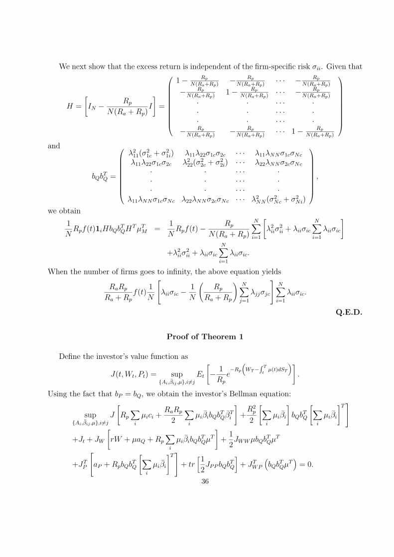
We next show that the excess return is independent of the firm-specific risk σii. Given that

H =

[IN − Rp

N(Ra + Rp)I

]=

1− Rp

N(Ra+Rp)− Rp

N(Ra+Rp)· · · − Rp

N(Ra+Rp)

− Rp

N(Ra+Rp)1− Rp

N(Ra+Rp)· · · − Rp

N(Ra+Rp)

· · · · · ·· · · · · ·· · · · · ·

− Rp

N(Ra+Rp)− Rp

N(Ra+Rp)· · · 1− Rp

N(Ra+Rp)

and

bQbTQ =

λ211(σ

21c + σ2

1i) λ11λ22σ1cσ2c · · · λ11λNNσ1cσNc

λ11λ22σ1cσ2c λ222(σ

22c + σ2

2i) · · · λ22λNNσ2cσNc

· · · · · ·· · · · · ·· · · · · ·

λ11λNNσ1cσNc λ22λNNσ2cσNc · · · λ2NN(σ2

Nc + σ2Ni)

,

we obtain

1

NRpf(t)1iHbQbT

QHT µTM =

1

NRpf(t)− Rp

N(Ra + Rp)

N∑i=1

[λ2

iiσ2ii + λiiσic

N∑i=1

λiiσic

]

+λ2iiσ

2ii + λiiσic

N∑i=1

λiiσic.

When the number of firms goes to infinity, the above equation yields

RaRp

Ra + Rp

f(t)1

N

λiiσic −1

N

(Rp

Ra + Rp

)N∑

j=1

λjjσjc

N∑i=1

λiiσic.

Q.E.D.

Proof of Theorem 1

Define the investor’s value function as

J(t,Wt, Pt) = sup{Ai,βij ,µ},i6=j

Et

[− 1

Rp

e−Rp

(WT−

∫ T

tµ(t)dST

)].

Using the fact that bP = bQ, we obtain the investor’s Bellman equation:

sup{Ai,βij ,µ},i6=j

J

[Rp

∑i

µici +RaRp

2

∑i

µiβibQbTQβT

i

]+

R2p

2

[∑i

µiβi

]bQbT

Q

[∑i

µiβi

]T

+Jt + JW

[rW + µaQ + Rp

∑i

µiβibQbTQµT

]+

1

2JWW µbQbT

QµT

+JTP

aP + RpbQbTQ

[∑i

µiβi

]T+ tr

[1

2JPP bQbT

Q

]+ JT

WP

(bQbT

QµT)

= 0.

36

The FOCs are given by

w.r.t. Ai:

JRp

[µikiAi + Ra

µi

λii

ki1ibQbTQβT

i + Rpµi

λii

ki1ibQbTQ

∑i

µiβTi

]

+JW

∑j

µjλji + Rpki

λii

1ibQbTQµT

+ JTP

λ11

λ21

···

λN1

+ RpbQbT

Q

1

λii

ki1ibQbTQµT

= 0,

where 1i denotes a row vector with the ith element being one and all other elements being

zero. w.r.t. µT :

J

Rp

c1

c2

···

cN

+

RaRp

2

β1bQbTQβT

1

β2bQbTQβT

2

···

βNbQbTQβT

N

+ R2

p

β1

β2

···

βN

bQbT

Q

[βT

1 βT2 · · · βT

N

]µT

+ JW

aQ + Rp

bQbT

Q

[βT

1 βT2 · · · βT

N

]+

β1

β2

···

βN

bQbT

Q

µT

+ Rp

β1

β2

···

βN

bQbT

QJP + JWW bQbTQµT + bQbT

QJWP = 0.

w.r.t. βij:

J

[Ra

[0 · · · −λji

λii· · · 1 · · · 0

]bQbT

QβTi + Rp

[0 · · · −λji

λii· · · 1 · · · 0

]bQbT

Q

∑i

µiβTi

]+JW

[[0 −λji

λii· · · 1 · · · 0

]bQbT

QµT]+[

0 −λji

λii· · · 1 · · · 0

]bQbT

QJP = 0,

where the ith element equals λji

λiiand the jth element equals 1.

Conjecture that the investor’s value function is given by

J = − 1

Rp

exp [−Rp (f(t)Wt + g(t))] ,

37

with the boundary conditions f(T ) = 1 and g(T ) = 0. The Bellman equation then becomes

sup{Ai,βij ,µ},i6=j

∑i

µici +Ra

2

∑i

µiβibQbTQβT

i +Rp

2

∑i

µiβibQbTQ

[∑i

µiβi

]T

− f(t)W − g(t)− f(t)

[rW + µaQ + Rp

∑i

µiβibQbTQµT

]+

Rp

2f 2(t)µbQbT

QµT

}= 0.

To satisfy the above Bellman equation, we obtain the following conditions:

f(t) + rf(t) = 0,

λii − (r − Πi) λii = 0,

λij − (r − Πi) λij = 0, i 6= j,

with boundary conditions f(T ) = 1 and λij(T ) = 0 for i = 1, 2, · · · , N and j = 1, 2, · · · , N . It

can be verified that the solutions are given by

f(t) = er(T−t), λij = 0, λii = e(r−Πi)(t−T ).

The first order conditions now reduce to

w.r.t. Ai:

µikiAi + Raµi

λii

ki1ibQbTQβT

i + Rpkiµi

λii

1ibQbTQ

[∑i

µiβi

]T

− f(t)[µiλii + Rp

µi

λii

ki1ibQbTQµT

]= 0.

w.r.t. µT :

c1

c2

···

cN

+

Ra

2

β1bQbTQβT

1

β2bQbTQβT

2

···

βNbQbTQβT

N

+ Rp

β1

β2

···

βN

bQbT

Q

[βT

1 βT2 · · · βT

N

]µT

−f(t)

aQ + Rp

bQbT

Q

[βT

1 βT2 · · · βT

N

]+

β1

β2

···

βN

bQbT

Q

µT

+ Rpf

2(t)bQbTQµT = 0.

w.r.t. βij:

Raµi1jbQbTQβT

i + Rpµi1jbQbTQ

∑i

µiβTi − f(t)

[Rpµi1jbQbT

QµT]

= 0.

38

In equilibrium, µi = 1N

. Using the FOCs with respect to µT , we getaQ −

1

f(t)

c1

c2

···

cN

+

Ra

2

β1bQbTQβT

1

β2bQbTQβT

2

···

βNbQbTQβT

N

=1

NRp

f(t)bQbT

QµTM +

1

f(t)

β1

β2

···

βN

bQbT

Q

[βT

1 βT2 · · · βT

N

]µT

M

−

bQbT

Q

[βT

1 βT2 · · · βT

N

]+

β1

β2

···

βN

bQbT

Q

µT

M

. (12)

Multiplying both sides by µM = (1 1 · · · 1), we have(aM

Q − 1

f(t)

[∑i

ci +Ra

2

∑i

βibQbTQβT

i

])

=1

NRpµM

f(t)bQbT

Q +1

f(t)

β1

β2

···

βN

bQbT

Q

[βT

1 βT2 · · · βT

N

]

− bQbTQ

[βT

1 βT2 · · · βT

N

]−

βT1

βT2

···

βTN

bQbT

Q

µT

M .

The above equation can also be expressed as:(aM

Q − 1

f(t)

∑i

[ci +

Ra

2βibQbT

QβTi

])

39

= Rpf(t)µM

IN − 1

f(t)

βT1

βT2

···

βTN

bQbT

Q

IN − 1

f(t)

βT1

βT2

···

βTN

T

µTM .

To find the expected excess return on stock i, adjusted for the manager’s expected com-

pensation, we multiply both sides of (12) by the 1i vector and have

Ei ≡(ai

Q −1

f(t)

(ci +

Ra

2βibQbT

QβTi

))

=1

NRpf(t)1i

IN − 1

f(t)

βT1

βT2

···

βN

bQbT

Q

IN − 1

f(t)

βT1

βT2

···

βN

T

µTM

= Rpf(t)1

N1iHbQbT

QHT µTM

= Rpf(t)1

NCov

[dPit −

1

f(t)dSiT ,

N∑i=1

(dPit −

1

f(t)dSiT

)]

= Rpf(t)1

NCov

[(1i −

1

f(t)βi

)bQdBt,

N∑i=1

(1i −

1

f(t)βi

)bQdBt

],

where matrix H is defined as:

H =

IN − 1

f(t)

βT1

βT2

···

βTN

.

Notice that Ei represents the expected excess dollar return on firm i adjusted for the

manager’s expected compensation. It can then be shown that

Ei =

[1iHbQbT

QHT µTM

µMHbQbTQHT µT

M

]EM =

Cov(dP adji , dP adj

M )

V ar(dP adjM )

EM ,

where dP adji = dPit − 1

f(t)dSiT and dP adj

M =∑N

i=1

(dPit − 1

f(t)dSiT

). This is a CAPM type

linear relation in terms of the expected dollar returns.

40

We next solve the FOCs with respect to Ai and βij for both the optimal effort and the

optimal contract in closed form. Start with the expression for bQbTQ:

bQbTQ =

λ211(σ

21c + σ2

1i) λ11λ22σ1cσ2c · · · λ11λNNσ1cσNc

λ11λ22σ1cσ2c λ222(σ

22c + σ2

2i) · · · λ22λNNσ2cσNc

· · · · · ·· · · · · ·· · · · · ·

λ11λNNσ1cσNc λ22λNNσ2cσNc · · · λ2NN(σ2

Nc + σ2Ni)

,

we obtain

1ibQbTQβT

i = λii

σic

N∑j 6=i

λjjσjcβij + (σ2ic + σ2

ii)kiAi

,

1jbQbTQβT

i = λjj

σjc

N∑l 6=i

λllσlcβil + σicσjckiAi + λjjσ2jiβij

,

1jbQbTQβT

j = λjj

σjc

∑i6=j

N∑i6=j

σicλiiβji + (σ2jc + σ2

ji)kiAi

,

1ibQbTQβT

j = λii

σic

N∑l 6=j

λllσlcβjc + λiiσ2iiβji + σjcσickjAj

,

1ibQbTQµT = λii

σic

N∑j=1

λjjσjc + λiiσ2ii

,

1jbQbTQµT = λjj

[σjc

N∑i=1

λiiσic + λjjσ2ji

].

The FOCs with respect to Ai and βij are now reduced to

kiAi + Raki

σic

N∑j 6=i

λjjσjcβij + (σ2ic + σ2

ii)kiAi

+

Rpki1

N

σic

N∑j 6=i

λjjσjcβij + (σ2ic + σ2

ii)kiAi

+N∑

j 6=i

σic

N∑l 6=j

λllσlcβjl + λiiσiiβji + σjcσickjAj

−f(t)

λii + Rpki1

N

σic

N∑j=1

λjjσjc + λiiσ2ii

= 0,

41

and

Ra

σjc

N∑l 6=i

λllσlcβil + σicσjckiAi + λjjσ2jiβij

+

Rp1

N

σjc

N∑i6=j

λiiβji + (σ2jc + σ2

ji)kjAj

+N∑

i6=j

σjc

N∑l 6=i

λllσlcβil + σicσjckaAi + λjjσ2jcβij

−f(t)Rp

1

N

[σjc

N∑i=1

λiiσic + λjjσ2ji

]= 0,

respectively.

Conjecture that βij, i 6= j, is given by

βij =1

N

[Rp

Ra + Rp

f(t)− kiAi

λjj

σic

σjc

],

where σic and σjc are nonzero, We now verify that this choice of βij satisfies the FOCs with

respect to βij:

Ra

σjc

N∑l 6=i

λllσlcRa

Ra + Rp

f(t)1

N − 1− σjc

N∑l 6=i

kiAiσic1

N − 1+ σjcσickiAi

+

Rp1

N

N∑i6=j

σjc

N∑l 6=i

λllσlcRp

Ra + Rp

f(t)1

N − 1− σjc

N∑l 6=i

kiAiσic1

N − 1+ σicσjckiAi

−f(t)Rp

1

Nσjc

N∑i=1

λiiσic

= RaσjcRp

Ra + Rp

f(t)1

N − 1

N∑l 6=i

λllσlc +R2

p

Ra + Rp

f(t)1

Nσjc

N∑l 6=i

λllσlc

−f(t)Rp1

Nσjc

N∑i=1

λiiσic

= f(t)1

N

[RaRp

Ra + Rp

+R2

p

Ra + Rp

−Rp

]σjc

N∑l 6=i

σllσlc = 0.

Notice that the expression for Ai is not required in the above derivation. Substituting βij

into the FOC with respect to Ai, we have

kiAi + Raki

σicRp

Ra + Rp

f(t)1

N − 1

N∑j 6=i

λjjσjc − σickiAiσic + (σ2ic + σ2

ii)kiAi

+

42

Rpki1

N

N∑

j 6=i

σic

N∑l 6=j

λllσlc

[Rp

Ra + Rp

f(t)− kjAj

λll

σjc

σlc

]1

N − 1+ σjcσickjAj

−f(t)

λii + Rpki1

Nσic

N∑j=1

λjjσjc

=

kiAi + Raki

Rp

Ra + Rp

f(t)1

N − 1σic

N∑j 6=i

λjjσjc + σ2iikiAi

+Rpki

1

N

N∑j 6=i

σic

N∑l 6=j

λllσlcRp

Ra + Rp

f(t)1

N − 1− f(t)

λii + Rpki1

Nσic

N∑j=1

λjjσjc

= 0,

where

RakiRp

Ra + Rp

f(t)1

N − 1σic

N∑j 6=i

λjjσjc + Rpki1

Nσic

Rp

Ra + Rp

f(t)N∑

l 6=j

λllσlc

−f(t)Rpki1

Nσic

N∑j=1

λjjσjc = 0.

We thus arrive at

A∗it =

f(t)λii

ki + Rak2i σ

2ii

=1

ki + Rak2i σ

2ii

e−Πi(t−T ),

which is independent of the market risk σic.

We next show that the expected excess dollar return on stock i is independent of the firm-

specific risk σii and that its equilibrium stock price decreases with σii. Recall that the excess

return can be expressed as

Ei = Rpf(t)1

NCov

[(1i −

1

f(t)βi

)bQdBt,

N∑i=1

(1i −

1

f(t)βi

)bQdBt

].

Straightforward calculation yields

bQdBt =

λ11σ1c λ1iσ1i 0 · · · 0 0λ22σ2c 0 λ22σ2i · · · 0 0· · · · · · · ·· · · · · · · ·· · · · · · · ·

λNNσNc 0 0 · · · 0 λNNσNi

dBct

dB1t

dB2t

···

dBNt

=

λ11(σ1cdBct + σ1t)λ22(σ2cdBct + σ2t)

···

λNN(σNcdBct + σNt)

,

43

1ibQdBt = λii(σidBct + σiidBit),

βidBt = βi1λ11(σ1cdBct + σ1idB1t) + βi2λ22(σ2cdBct + σ2idB2t) + · · ·

+kiAi(σicdBct + σiidBit) + · · ·+ βiNλNN(σNcdBct + σNidBNt),

where βi =(βi1, βi2, · · · , kiAi

λii, · · · , βiN

)and βij = 1

N−1

[Rp

Ra+Rpf(t)− kiAi

λjj

σic

σjc

]. We then have

(1i −

1

f(t)βi

)bQdBt = λii(σicdBct + σiidBit)−

1

f(t)βi1(λ11σ1cdBct + σ1idB1t)

− 1

f(t)βi2(λ22σ2cdBct + σ2idB2t)− · · · − kiAi

f(t)(σicdBct + σ1idBit)− · · ·

− 1

f(t)βiN(λNNσNcdBct + σNidBNt)

= λii(σicdBct + σiidBit)−[

Rp

Ra + Rp

− 1

f(t)

kiAi

λ11

σic

σ1c

]λ11

1

N − 1(σ1cdBct + σ1idB1t)

−[

Rp

Ra + Rp

− 1

f(t)

kiAi

λ22

σic

σ2c

]λ22

1

N − 1(σ2cdBct + σ2idB2t) · · ·

−kiAi(σicdBct + σiidBit)− · · ·

−[

Rp

Ra + Rp

− 1

f(t)

kiAi

λNN

σic

σNc

]λNN

1

N − 1(σNcdBct + σNidBNt)

= λii(σicdBct + σiidBit)−Rp

Ra + Rp

1

N − 1

N∑j 6=i

λjjσjcdBct −1

f(t)kiAiσ1idBit

=

λiiσic −Rp

Ra + Rp

1

N − 1

N∑j 6=i

λjjσjc

dBct +Rakiλiiσ

3ii

1 + Rakiσ2ii

dBit,

andN∑

i=1

(1i −

1

f(t)βi

)bQdBt =

Rp

Ra + Rp

N∑i=1

λiiσicdBct +N∑

i=1

Rakiλiiσ3ii

1 + Rakiσ2ii

dBit.

Consequently, we arrive at the expected excess dollar return:

Ei = Rpf(t)1

N

Ra

Ra + Rp

λiiσic −Rp

Ra + Rp

1

N − 1

N∑j 6=i

λjjσjc

N∑i=1

λiiσic.

Finally, we show that the equilibrium price decreases with the firm specific risk σii. Since

λii(t) is independent of σii, we only need to show that λi0(t) is a decreasing function of σii.

Recall that the expected excess return Ei is defined as

Ei = aiQ −

1

f(t)

[1

2kiA

2i +

Ra

2βibQbT

QβTi

],

44

where aiQ = λi0 − rλi0 + λiiAi. Our calculation yields

βibQbTQβT

i = βi1

N∑j 6=1

βijλ11λjjσ1cσjc + βi1λ211(σ

21c + σ2

1i) + kiAiλ11σ1cσic

+

βi2

N∑j 6=2

βijλ22λjjσ2cσjc + βi2λ222(σ

22c + σ2

2i) + kiAiλ22σ2cσic

+ · · ·

kiAi

λii

N∑j 6=i

βijλiiλjjσicσjc + kiAiλii(σ2ic + σ2

ii)

+ · · ·

= βi1

λ11σ1c

N∑j 6=i

βijλjjσjc + βi1λ211σ

21i + kiAiλ11σ1cσic

+

βi2

λ22σ2c

N∑j 6=i

βijλjjσjc + βi2λ222σ

22i + kiAiλ11σ1cσic

+ · · ·

kiAi

λiiσic

N∑j 6=i

βijλjjσjc + kiAi(σ2ic + σ2

ii)

+ · · ·

=1

N − 1

Rp

Ra + Rp

f(t)N∑l 6=i

λllσll

N∑j 6=i

βijλjjσjc +N∑

j 6=i

β2ijλ

2jjσ

2ji + (kiAi)

2σ2ii

⇒ (kiAi)2σ2

ii,

where we have ignored all the terms independent of σii. The expression for Ei then yields

Ei = λi0 − rλi0 + λiiAi −1

f(t)

[1

2kiA

2i +

Ra

2βibQbT

QβTi

]

= λi0(t)− rλi0(t) +

[λii −

1

f(t)

(1

2ki(1 + Rakiσ

2ii)Ai

)]Ai

= λi0(t)− rλi0(t) +1

2λii.

Ignoring the terms independent of σii and solving the above ordinary differential equation, we

get

λi0(t) =1

2ert∫ T

t

e−Π(u−T )eru

ki(u) + Rak2i (u)σ2

ii

du,

which is clearly a decreasing function of σii. Q.E.D.

Proof of Theorem 2

In the absence of relative performance evaluation, βi is given by βi =(0, · · · , kiAi

λii, · · · , 0

).

We then have

1ibQbTQβT

i = λii(σ2ic + σ2

ii)kiAi, 1ibQbTQβT

j = λiiσicσjckjAj,45

1ibQbTQ

N∑j=1

βTi = λiiσ

2iikiAi +

N∑j=1

λiiσicσjckjAj, 1ibQbTQµT =

1

Nλiiσic

N∑j=1

λjjσjc.

Substituting the above relations into the FOC with respect to Ai, we have42

kiAi + Rak2i (σ

2ic + σ2

ii)Ai +1

NRpki

N∑j=1

σicσjckjAj − f(t)

λii +1

NkiRpσic

N∑j=1

λjjσjc

= 0.

We next show that if σlc = σic = σc, kl = ki = k, Πl = Πi, and σli > σii, then Al < Ai. To

do so, we subtract the FOC with respect to Al from the FOC with respect to Ai, yielding,

k(Ai − Al) + Rak2[σ2

c (Ai − Al) + σ2iiAi − σ2

liAl

]= 0.

Suppose that Ai ≥ Al, it is easy to see that the above equality would not hold, thus proving

the claim.

Since the cross terms in the β matrix vanish in the absence of RPE, the H matrix that

appears in the expected excess dollar return is diagonal given by

H =1

f(t)

f(t)− β11 0 · · · 0 0

0 f(t)− β22 · · · 0 00 · · · f(t)− βii 0 00 0 · · · 0 f(t)− βNN

,

where βii = kiAi

λii. It can then be shown that the excess return is given by

Ei = Rpf(t)1

N1iHbQbT

QHT µTM

= Rp1

f(t)

1

N

[f(t)− kiAi

λii

]λiiσic

N∑j=1

λjjσjc

[f(t)− kiAi

λii

].

It can be shown that f(t) ≥ kiAi

λii.

Finally, we show that the equilibrium price is a decreasing function of the firm-specific risk

σii. Straightforward calculation yields

βibQbTQβT

i = k2i A

2i (σ

2ic + σ2

ii).

We then have

Ei = λi0 − rλi0 + λiiAt −1

f(t)

[1

2kiA

2i +

Ra

2βibQbT

QβTi

]= λi0 − rλi0 + λiiAt −

1

f(t)

[1 + Raki(σ

2ic + σ2

ii)] 1

2kiA

2i

42Without RPE, the FOC with respect to βij vanishes from the investor’s problem.

46

= λi0 − rλi0 +

{λii −

1

2ki

1

f(t)

[1 + Raki(σ

2ic + σ2

ii)]Ai

}Ai

= λi0 − rλi0 +1

2λiiAi −

1

NkiRpσicAi

N∑j=1

σjc

[λjj −

kjAj

f(t)

].

Substituting the expression for Ei into the above equation, we obtain

λi0 − rλi0 = −1

2λiiAi +

1

NkiRpσicAi

N∑j=1

σjc

[λjj −

kjAj

f(t)

]

=Rp

f(t)

1

N

[f(t)− kiAi

λii

]λiiσic

N∑j=1

σjcλjj

[f(t)− kjAj

λjj

]

= −1

2λiiAi + Rp

1

Nλiiσic

N∑j=1

σjcλjj

[f(t)− kjAj

λjj

],

where the second term on the right hand side is independent of σii. Ignoring this term, we

arrive at

λi0(t) =1

2ert∫ T

teruλii(u)Ai(u)du,

which is a decreasing function of σii due to the fact that Ai(t) decreases with σii. Q.E.D.

47

References

Abowd, J.M., and D.S. Kaplan, 1999, Executive compensation: six questions that need an-swering, Journal of Economic Perspectives, 13, 145-168.

Admati, A., 1985, A noisy rational expectations equilibrium for multi-asset securities markets,Econometrica, 53, 629-658.

Aggarwal, R., and A. Samwick, 1999a, The other side of the trade-off: The impact of risk onexecutive compensation, Journal of Political Economy, 107, 65-105.

Aggarwal, R., and A. Samwick, 1999b, Executive compensation, strategic competition, andrelative performance evaluation: Theory and evidence, Journal of Finance, 54, 1999-2043.

Allen, F., 2001, Do financial institutions matter? Journal of Finance, 56, 1165-1175.

Antle, R., and A. Smith, 1986, An empirical investigation of the relative performance evalua-tion of corporate executives, Journal of Accounting Research, 24, 1-39.

Arora, N., and H. Ou-Yang, 2001, A model of asset pricing and portfolio delegation, workingpaper, Duke University and KMV.

Baiman, S., and J. Demski, 1980, Economically optimal performance evaluation and controlsystems, Journal of Accounting Research, Supplement.

Barro, J., and R.J. Barro, 1990, Pay, performance, and turnover of bank CEOs, Journal ofLabor Economics, 8, 448-481.

Bertrand, M., and S. Mullainathan, 1999, Are CEOs rewarded for luck? A test of performancefiltering, Quaterly Journal of Economics, forthcoming.

Breeden, D., 1979, An intertemporal asset pricing model with stochastic consumption andinvestment opportunities, Journal of Financial Economics, 7, 265-296.

Brennan, M.J., 1993, Agency and asset pricing, working paper, University of California, LosAngeles.

Campbell, J.Y., M. Lettau, B.G. Malkiel, and Y. Xu, 2001, Have individual stocks becomemore volatile?, Journal of Finance, 56, 1-43.

Campbell, J.Y., and A.S. Kyle, 1993, Smart money, noise trading and stock price behavior,Review of Economic Studies, 60, 1-34.

Cochrane, J.H., 2001, Asset Pricing, Princeton University Press.

Core, J.E., G. Wayne, and D.F. Larcker, 2001, Executive equity compensation and incentives,A survey, working paper, University of Pennsylvania.

Dai, Q., 2002, Asset pricing in a neoclassical model with limited participation, working paper,New York University and Stanford University.

DeMarzo, P.M., and B. Urosevic, 2001, Optimal trading by a “large shareholder”, workingpaper, Stanford University and University of California, Berkeley.

Diamond, D.W., and R.E. Verrecchia, 1982, Optimal managerial contracts and equilibriumsecurity prices, Journal of Finance, 37, 275-287.

Diamond, D.W., and R.E. Verrecchia, 1991, Disclosure, liquidity, and the cost of capital,Journal of Finance, 46, 1325-1359.

Duffie, D., 2001, Dynamic Asset Pricing Theory, Princeton University Press.

48

Duffie, D., W. Fleming, H.M. Soner, and T. Zariphopoulou, 1997, Hedging in incompletemarkets with HARA utility, Journal of Economic Dynamics and Control, 21, 753-782.

Easley, D., and M. O’Hara, 2001, Information and the cost of capital, working paper, CornellUniversity.

Gibbons, R., and K. Murphy, 1990, Relative performance evaluation for chief executive officers,Industrial and Labor Relations Review, 43, 30s-52s.

Goyal, A., and P. Santa-Clara, 2001, Idiosyncratic risk matters, working paper, University ofCalifornia, Los Angeles.

He, H., and J. Wang, 1995, Differential information and dynamic behavior of stock tradingvolume, Review of Financial Studies, 8, 919-972.

Heaton, J., and D. Lucas, 2000, Portfolio choice and asset prices: The importance of en-trepreneurial risk, Journal of Finance, 55, 1163-1198.

Himmelberg, G.P., and R.G. Hubbard, 2000, Incentive pay and the market for CEOs: Ananalysis of pay-for-performance sensitivity, working paper, Columbia University.

Holmstrom, B., 1982, Moral Hazard in Teams, Bell Journal of Economics, 13, 324-340.

Holmstrom, B., and P. Milgrom, 1987, Aggregation and linearity in the provision of intertem-poral incentives, Econometrica, 55, 303-328.

Ingersoll, J.E., 1987, Theory of Financial Decision Making, Rowman & Littlefield, New Jersey.

Janakiraman, S., R. Lambert, and D. Larcker, 1992, An empirical investigation of the relativeperformance evaluation hypothesis, Journal of Accounting Research, 30, 53-69.

Jensen, M., and K. Murphy, 1990, Performance pay and top-management incentives, Journalof Political Economy, 98, 225-264.

Jin, L., 2001, CEO compensation, diversification and incentives, working paper, MIT.

Kahn, J.A., 1990, Moral hazard, imperfect risk-sharing, and the behavior of asset returns,Journal of Monetary Economics, 26, 27-44.

Karatzas, I., and S.E. Shreve, 1991, Brownian motion and stochastic calculus, Springer-Verlag.

Kihlstrom, R.E., and S.A. Matthews, 1990, Managerial incentives in an entrepreneurial stockmarket model, Journal of Financial Intermediation, 1, 57-79.

Kocherlakota, N.R., 1998, The effects of moral hazard on asset prices when financial marketsare complete, Journal of Monetary Economics, 41, 39-56.

Leland, H.E., and D. Pyle, 1977, Information asymmetries, financial structure, and financialintermediation, Journal of Finance, 32, 371-387.

Lintner, J., 1965, The valuation of risky assets and the selection of risky investments in stockportfolios and capital budgets, Review of Economics and Statistics, 47, 13-37.

Liu, J., 2001, Portfolio selection in stochastic environments, working paper, University ofCalifornia, Los Angeles.

Lo, A.W., and J. Wang, 2001, Trading volume: Implications of an intertemporal capital assetpricing model, working paper, Massachusetts Institute of Technology.

Lucus, R., 1978, Asset prices in an exchange economy, Econometrica, 46, 1429-1445.

Magill, M., and M. Quinzii, 2000, Capital market equilibrium with moral hazard, workingpaper, USC and UC Davis.

49

Malkiel, B.G., and Y. Xu, Spring 1997, Risk and return revisited, Journal of Portfolio Man-agement, 9-14.

Malkiel, B.G., and Y. Xu, 2000, Idiosyncratic risk and security returns, working paper, Uni-versity of Texas at Dallas.

Merton, R., 1971, Optimum consumption and portfolio rules in a continuous time model,Journal of Economic Theory, 3, 373-413.

Merton, R., 1973, An intertemporal capital asset pricing model, Econometrica, 41, 867-888.

Mirrlees, J.A., 1974, Notes on welfare economics, information, and uncertainty, in M. Balch,D. McFadden, and S. Wu (Eds.) Essays in Economic Behavior under Uncertainty, 243-258.

Mossin, J., 1966, Equilibrium in a capital asset market, Econometrica, 35, 768-783.

Murphy, K., 1999, Executive compensation, in Orley Ashenfelter and David Card (eds.),Handbook of Labor Economics, Vol. 3, North Holland.

Ou-Yang, H., 2000, Optimal contracts in a continuous-time delegated portfolio managementproblem, Review of Financial Studies, Forthcoming.

Prendergast, C., 1999, The provision of incentives in firms, Journal of Economic Literature,37, 7-63.

Ramakrishnan R.T.S., and A.V. Thakor, 1982, Moral hazard, agency costs, and asset pricesin a competitive equilibrium, Journal of Financial and Quantitative Analysis, 17, 503-532.

Ramakrishnan R.T.S., and A.V. Thakor, 1984, The valuation of assets under moral hazard,Journal of Finance, 34, 229-238.

Roll, R., 1977, A critique of the asset pricing theory’s tests; part I: On past and potentialtestability of the theory, Journal of Financial Economics, 4, 129-176.

Ross, S., 1976, The arbitrage pricing theory, Journal of Economic Theory, 13, 341-360.

Rubinstein, M., 1976, The valuation of uncertain income streams and the pricing of options,Bell Journal of Economics, 7, 407-425.

Schattler, H., and J. Sung, 1993, The first-order approach to the continuous-time principal-agent problem with exponential utility, Journal of Economic Theory, 61, 331-371.

Sharpe, W.F., 1964, Capital asset prices: A theory of market equilibrium under conditions ofrisk, Journal of Finance, 19, 425-442.

Sloan, R., 1993, Accounting earnings and top executive compensation, Journal of Accountingand Economics, 16, 55-100.

Stulz, R.M., 1999, What’s wrong with modern capital budgeting? Financial Practice andEducation, Fall/Winter, 5-9.

Storesletten, K., C.I. Telmer, and A. Yaron, 2001, Asset pricing with idiosyncratic risk andoverlapping generations, working paper, Carnegie-Mellon University and University of Penn-sylvania.

Urosevic, B., 2001, Dynamics of corporate insider ownership: theory and evidence, workingpaper, University of California, Berkeley.

Wang, J., 1993, A model of intertemporal asset prices under asymmetric information, Reviewof Economic Studies, 60, 249-282.

Wilson, R.B., 1968, on the theory of syndicates, Econometrica, 36, 119-132.

50