1

An Empirical Test for Inter-State Carbon-Dioxide Emissions Leakage Resulting from the Regional Greenhouse Gas Initiative

Andrew G. Kindle and Daniel L. Shawhan Rensselaer Polytechnic Institute Michael J. Swider New York Independent System Operator, Inc.

April 20, 2011

2

Summary At the request of market participants, the New York Independent System Operator Inc. (NYISO) undertook the task of developing a methodology to evaluate whether the cost of compliance with the Regional Greenhouse Gas Initiative (RGGI) has caused an increase in emissions in neighboring non-RGGI areas such as Pennsylvania. An increase in emissions, sometimes termed “leakage,” can be caused by a shift in the relative economics of generating power in RGGI and non- RGGI states. In order to test for such an increase, the NYISO together with researchers at Rensselaer Polytechnic Institute (RPI) developed econometric models to explain both power transfers between New York and Pennsylvania and carbon dioxide (CO2) emissions from power plants in Pennsylvania. These models estimate the effect on these two variables from variations in RGGI allowance prices, electrical load, fuel prices, nitrogen oxide and sulfur dioxide allowance prices, temperature, production from non-emitting generation, and New England-to-New York power transfers. If, in these models, a higher RGGI allowance price were empirically associated with higher Pennsylvania-New York power flows or Pennsylvania emissions, that would indicate RGGI emissions leakage. Other studies have modeled system-wide emissions leakage from the RGGI program or considered the effect of a proposed transmission line on leakage. The difference between these studies and ours is that the previous studies were prospective and employed simulations, while ours is retrospective and employs statistical analysis of historical data. Our econometric analysis does not support the hypothesis that RGGI compliance cost in New York has caused emissions leakage. The period evaluated was from 2008 through September 2010. Variables such as electrical loads, fuel costs, and non-emitting generation were, as expected, all shown to have statistically significant impacts on emissions, Pennsylvania-to-New York power transfers, or both. However, the models were not able to show a statistically significant impact from RGGI costs on either of these variables. RGGI prices appear to have been too low from the start of the program in 2009 to have a significant effect on emissions leakage from New York to Pennsylvania. It is not possible to measure all factors that can influence power transfers or emissions, or to represent in an econometric model the exact nature of the influence that the measured factors exert. In the past decade CO2 emissions have trended lower in both New York and Pennsylvania. These reductions are largely due to cyclical and secular changes in supply and demand for electric power. Some of these changes have been large, and likely contribute to the difficulty of detecting a subtle phenomenon such as emissions leakage from RGGI. Differing market rules between areas can also reduce the price arbitrage opportunities that would otherwise be available, and hence the response of Pennsylvania-New York flows to a RGGI-induced increase in New York’s marginal cost of generation.

3

Background

The ten Regional Greenhouse Gas Initiative (RGGI) states1 have committed to a CO2

budget and trading program aimed at stabilizing and then reducing CO2 emissions from

fossil-fueled electricity generating units having a rated capacity equal to or greater than

25 megawatts (“CO2 budget sources” or “sources”). This program went into effect on

January 1, 2009. RGGI requires all sources to ultimately possess CO2 allowances equal

to their CO2 emissions over a three-year control period.

The member states in RGGI auction off, or in some cases give away, allowances that

permit CO2 emissions in the electricity sector. Once auctioned, allowances may be re-

sold in secondary markets. The need for these allowances increases the marginal cost

per MWh of generators having to purchase them, in proportion to their CO2 emissions

per MWh. This applies even to firms already holding enough allowances to meet their

requirements, because each allowance they have to retain reduces the number of

allowances they can sell at the prevailing allowance price in the secondary market.

If the cost of RGGI compliance causes load-serving entities in participating states to

import more power from non-participating states and provinces, and if the incremental

generation in those non-participating states produces CO2 emissions, the result is inter-

regional emissions leakage. Any leakage would counteract emission reductions gained

in the RGGI states, thereby reducing the effectiveness of the RGGI program at lowering

total CO2 emissions. RGGI leakage can be defined as a RGGI-induced shift of electricity

production from generators subject to RGGI to CO2-emitting generators not subject to

RGGI.

The CO2 emission reductions resulting from RGGI can be decomposed into short-run and

long-run effects. Long-run effects can be changes in demand and changes in the supply

portfolio. This study does not try to estimate long-run effects because of the lack of

long-run historical data. However, sufficient data exists to look for short-run effects,

which can be supply-side or demand-side.

Short-run supply-side effects a. In RGGI states: The need to hold one allowance for every ton of CO2 emitted

reduces emissions by raising the marginal generation costs, and hence the offer prices, of higher-emitting generators more than those of lower-emitting

1 New York, New Jersey, Massachusetts, Maine, New Hampshire, Vermont, Connecticut, Rhode Island,

Delaware and Maryland.

4

generators and of generators not subject to the allowance requirement, such as those in Pennsylvania. This causes higher-emitting generators subject to the allowance requirement to be used less.

b. In neighboring jurisdictions: Since RGGI raises the offer prices of emitting generators subject to its allowance requirement, generators not subject to the requirement, such as those in neighboring states and provinces, are used more. This increases their emissions. This is leakage.

Short-run demand-side effects

c. In RGGI states: By raising the offer prices of generators, RGGI raises the market price of electricity, which induces an immediate reduction in consumption.

d. In neighboring jurisdictions: The higher offer prices within RGGI (a form of supply reduction) increase RGGI states’ demand for electricity from neighboring jurisdictions. This reduces the residual supply of generation in those jurisdictions, which may drive up the price and reduce consumption in those jurisdictions. This would result in a reduction of emissions, and so can be called “negative leakage.”

The short-run effects can be expected to affect emissions and power flows in proportion

to the then-current RGGI allowance price. However, the short-run demand-side effect is

reflected in load. Therefore, if one tests for an effect of the RGGI allowance price on

Pennsylvania-New York power flows or on Pennsylvania CO2 emissions, and controls for

load as one must, the type of leakage that remains to detect is short-run supply-side

leakage, which is the short-run supply-side effect in jurisdictions neighboring the RGGI

states. This is the most direct type of leakage, and it is what we attempt to detect in

recent historical data. The long-run leakage effects accumulate over the years rather

than being a daily function of the current RGGI allowance price, and attempting to

measure any of them would require a longer time period of historical data and a

different approach than the one we employ to measure short-run leakage.

Review of Previous RGGI Leakage Studies

An established strain of academic literature uses economic models to predict emissions

leakage between nations (e.g. Paltsev 2001). The phenomenon is not limited to CO2 or

to the electricity sector. Emissions leakage can occur when emissions raise the marginal

production cost of a tradable good in one region but not in another, such as when one

region has a cap-and-trade program on emissions from industry but another region does

not.

5

In the electricity sector, factors such as transmission constraints can limit emissions

leakage. Transmission thermal ratings and system stability requirements limit the

amount of electric power that can be imported into New York, regardless of short-run

economics. For example, total transfer capability for imports from the PJM

Interconnection are typically limited to a range of 2,800 to 3,660 MW.2

As discussed below, two previous studies have modeled system-wide emissions leakage

from the RGGI program, and another has considered the effect of a proposed

transmission line on leakage. The difference between the earlier studies and our study

is that earlier studies were prospective and employed simulations, while ours is

retrospective and employs statistical methods to attempt to identify actual RGGI

impacts.

ICF Study

At the request of RGGI Inc, ICF International used its Integrated Planning Model (IPM©)

to predict emissions leakage from RGGI through 2024. This model includes many input

variables including the costs of different types of new power plants and power plant

retrofits, air policy specifications, resource supplies, operational factors such as

maintenance requirements, existing power plant variable costs, electricity demand, and

transmission capabilities. The IPM uses a “pipe-and-bubble” (EIPC 2010) model of the

transmission system: the US and Canada are divided into regions (eight for RGGI), there

are no transmission constraints within the regions, and there are fixed MW flow

constraints between the regions. The model uses all of these inputs to predict power

plant investment and retirement, power plant dispatch, power prices, fuel prices,

allowance prices, emissions in each region, and other future variables (ICF Consulting

2006a, pp. 10 and 12). Because the IPM predicts investment in and retirement of

generators, the ICF prediction of RGGI leakage includes not just short-run supply-side

leakage but also the long-run supply-side effects. The model also includes demand-side

effects.3

The ICF study compared a business-as-usual case which used middle-of-the-road

forecasts of future variables with a case that includes the RGGI policy. The model

predicted that RGGI CO2 emission allowance prices would remain in the range of $2-$3

per short ton through 2015 (ICF Consulting 2006b, p. 8). Net electricity imports to the

2 http://mis.nyiso.com/public/P-8list.htm

3 As indicated by the fact that predicted electricity consumption is lower in the RGGI case than in the

business-as-usual case (RGGI 2006b, p. 6).

6

RGGI states4 are higher in the RGGI case than in the business-as-usual case, and

cumulative inter-regional emissions leakage is estimated at 27% of net cumulative RGGI

CO2 emission reductions through 2015 (RGGI Inc 2007a). This means that emissions

increases in non-participating states are predicted to increase by 27% of the RGGI

reductions, where the RGGI reductions are net power plant CO2 emission reductions

resulting from RGGI in the RGGI states plus CO2 emission reductions from offsets.

Offsets are extra allowances earned by sponsoring projects that reduce greenhouse gas

emissions from sources other than power plants (RGGI Inc 2007b). If offsets are

excluded from the calculation or RGGI reductions, inter-regional leakage is

approximately 50% or RGGI reductions (ICF Consulting 2006b, p. 12). Because the ICF

estimates of emission reductions may not include some of the demand-side effects of

RGGI on emissions, they may be an incomplete prediction of total emission reductions.

As a result, these ICF leakage predictions may overstate leakage as a percentage of

emission reductions.

The ICF study predicts that most of the leakage will be a result of a long-run supply-side

effect: investors choosing to locate new combined cycle gas-fired generators outside of

RGGI rather than inside of RGGI. The Initial Report of the RGGI Emissions Leakage Multi-

State Staff Working commented on this prediction, calling it “an outcome that Staff

deems to be unlikely in the real world” (RGGI Inc 2007a).

In addition, the ICF simulation predicts that most of the leakage would occur in non-

RGGI PJM states, such as Pennsylvania, rather than in Canadian provinces or in non-PJM

US states. The RGGI Staff Working Group concluded that given the limitations in the

model, and the uncertainty about its investment prediction, “there is insufficient

information to make refined estimates as to the potential amount of emissions leakage

that may occur over the course of the program.”

Cornell-RPI Study

Shawhan, Mitarotonda, Zimmerman, and Taber (2010) estimate the short-run supply-

side inter-regional effects of RGGI using a more complex representation of the

transmission system. They assemble and employ a 36-node alternating-current optimal-

power-flow model of the power grid in northeastern North America. Their model

predicts that, with the current transmission system and generators, and non-price-

responsive demand, a RGGI allowance price of $3.87 leads to an immediate emission

reduction in RGGI states of 1.6 million metric tonnes per year. This is an estimate of the

4 Henceforth, the term “RGGI states” shall refer to the ten participating states as well as to the District of

Columbia, which is participating.

7

short-run supply-side effect of RGGI on emissions within the RGGI states. Their model

estimates an accompanying CO2 immediate emission increase in surrounding states and

provinces of 1.3 million metric tonnes.5 Therefore, they estimate that the short-run

supply-side effect of RGGI on CO2 emissions is subject to 82% leakage (Shawhan et al.

2010, p. 18). Because this study includes only the short-run supply-side effects of RGGI

on emissions, it predicts only a portion of the total emission reductions from RGGI. As a

percentage of the total RGGI-induced emission reductions, the emission increase in

neighboring states and provinces (i.e. inter-regional leakage) could be expected to be

smaller than 82%, perhaps much smaller. For this same reason, the Shawhan et al.

estimate is not inconsistent with the ICF estimate, since the ICF estimate includes more

components of the total emission reductions that can be expected to result from RGGI.

Since the start of the initial compliance period on January 1, 2009, the price in the

secondary market for RGGI allowances has never been higher than $4.13. In the most

recent auctions, the allowances have sold for $1.86, which is the reserve price. The

figure below shows a history of RGGI allowance prices from one month prior to the date

that the allowance requirement took effect. It reveals that the allowance price

prediction of the ICF study and the allowance price assumption of the Shawhan et al

study have approximately correct magnitudes.

5 This is the same type of leakage that we attempt to detect and measure in the present study. This

estimate of 1.3 million tonnes per year is short-run supply-side leakage in all neighboring states and provinces, while we attempt to detect only the portion in the important neighboring state of Pennsylvania.

8

$-

$0.50

$1.00

$1.50

$2.00

$2.50

$3.00

$3.50

$4.00

$4.50

12/1/08 3/11/09 6/19/09 9/27/09 1/5/10 4/15/10 7/24/10 11/1/10

RGGI Auction and Secondary Market Prices

Secondary Market Current Period Auction Future Period Auction Reserve Price

Sources: www.rggi.org and www.ccfe.com

PSEG Study

The Public Service Electric and Gas Company (PSEG) performed a study to determine the

CO2 emissions impact of their proposed Susquehanna-Roseland transmission line

connecting Pennsylvania to New Jersey. The analysis used the production cost modeling

software PROMOD,6 with a detailed security-constrained unit commitment and dispatch

module. The base simulations assumed PJM’s 2013 projection of peak load and

assumed that RGGI would be in effect. This analysis predicted that the Susquehanna-

Roseland line would, in the base case, decrease emissions in the RGGI region by 218,862

tons and increase emissions outside of RGGI by 353,189 tons, for a net increase of

134,336 tons in PJM, which is 0.03% of the overall CO2 emissions in PJM. A second case

assumed a national CO2 price instead of RGGI in order to isolate the emission effect of

the line not attributable to its interaction with the RGGI policy. This scenario estimated a

net increase of 64,403 tons CO2. Hence, about half of the line’s impact on emissions

would occur in the absence of the RGGI policy. This indicates that about half of the

line’s effect on power transfers from Pennsylvania to New Jersey, and on emissions, in

the base (RGGI) case are due to fuel cost differentials, rather than RGGI compliance

6 http://www.ventyx.com/analytics/promod.asp

9

costs.7 While this analysis only considered the effects of the new transmission line, it

shows that the low-cost coal power in western PJM creates an economic incentive to

transmit more emissions-intensive power from Pennsylvania if the transmission system

will allow it. In the analysis, the change in emissions in each area comes mostly from

combined-cycle gas unit output in RGGI states being replaced with coal unit output in

Pennsylvania. In this case the net emission increase is caused by the removal of

transmission congestion.

Econometric Analysis of RGGI Leakage

For our analysis we empirically test for CO2 emissions leakage from the RGGI states to

Pennsylvania, which is not a member of RGGI. If the ICF study is correct in its prediction

that most of the leakage will occur in non-RGGI PJM states, then it seems likely that

much of it will occur in Pennsylvania, since Pennsylvania is the non-RGGI PJM state in

closest proximity to most of the RGGI states, and has an abundance of coal-fired

generation capacity.

Unlike previous studies on leakage that have used production cost models with

representations of transmission topology to estimate leakage under various scenarios,

this study attempts to directly measure emissions leakage by examining historical data.

An empirical relationship between the RGGI allowance price and either Pennsylvania

emissions or scheduled power imports from Pennsylvania to a RGGI state, controlling for

other factors, would indicate emissions leakage. Our study evaluated scheduled flows

rather than actual flows because schedules should more accurately reflect the economic

evaluation of power costs between regions than actual flows. System operators

dispatch the power system to match actual flows to schedules; but unanticipated events

can cause actual power flows to somewhat deviate from scheduled transactions,

causing random, counter-intuitive flows.

Changes in emissions that result from the low RGGI allowance prices are likely to be

difficult to separate from other factors that influence emissions. One reason is the

magnitude of the RGGI allowance price relative to the price of electricity. If the typical

marginal generation unit in the RGGI states has a marginal emission rate of 0.5 tons per

MWh and the RGGI allowance price is $2 per ton, then the effect on the marginal

generation cost of that marginal unit is $1 per MWh. This is small relative to the

7 Public Service Electric and Gas, in New Jersey BPU Docket EM00010035, Exhibit SRTT-114

10

average wholesale cost of electricity. For example, the average wholesale cost in the

NYISO in 2010 was $58.92. Another reason for the difficulty of detecting statistically

significant effects of the RGGI allowance price is the large variations in other variables

that are likely to also affect net imports to the RGGI states and emissions in neighboring

jurisdictions. From 2005 to 2009, carbon dioxide emissions decreased by 33 percent in

the RGGI region.8 Identified reasons are decreases in load, fuel switching from

petroleum and coal sources to natural gas, and changes in capacity mix from increases

in wind, nuclear, and hydropower. Absent large changes in the emission characteristics

of generators, electrical load is the major determinant of the quantity of carbon dioxide

emissions.

Analysis of Scheduled Flows from Pennsylvania to New York

Our first means to test for emissions leakage is to attempt to detect a statistically

significant effect of RGGI allowance prices on power flows between Pennsylvania and

New York. New York shares seven high-voltage interties with Pennsylvania, which has an

electric supply mix dominated by coal generation and is ranked second in the nation for

CO2 emissions.9 Power can also flow from Pennsylvania to New York through New

Jersey, which is a RGGI state. However, we chose to test our methodology only on flows

that can be directly measured. New York is also interconnected with Ontario and

Quebec. While neither is a member of RGGI, the electric energy in these Provinces is

primarily from non-emitting sources such as hydroelectric and nuclear power

generators. Finally, New York is also interconnected with the other RGGI states of

Massachusetts, Connecticut, and Vermont.

Higher net flows from Pennsylvania to New York associated with higher RGGI allowance

prices would indicate emissions leakage. This assumes that some of the additional

generation in Pennsylvania would produce emissions, but that is virtually certain. In

PJM, the regional system that includes Pennsylvania, a coal-burning unit was the

marginal unit 74% of the time and a gas-burning unit was the marginal unit 22% of the

time (Monitoring Analytics 2010).

8 Relative Effects of Various Factors in RGGI Electricity Sector CO2 Emissions: 2009 Compared to 2005,

Prepared by NYSERDA for RGGI Inc., November 2010 9 http://tonto.eia.doe.gov/state/state_energy_rankings.cfm?keyid=86&orderid=1

11

Data Selection and Description for Scheduled Flows Analysis

We estimate a model that predicts scheduled flow of electric energy (i.e. external

transactions) across the Pennsylvania-New York border, with the RGGI allowance price

as one of the explanatory variables. If the coefficient on the RGGI permit price were

positive and statistically significant, it would be empirical evidence of CO2 emissions

leakage from the RGGI states to Pennsylvania.

A weekly time step is used because of the high variability in daily scheduled flows that

we cannot explain well. There are many cases of 100 percent increases or 50 percent

decreases in flows from one day to the next which may result from influential but

difficult-to-measure events. This is true of both the real-time and day-ahead scheduled

flows.

We try both day-ahead scheduled flow and real-time scheduled flow as our dependent

variable, i.e. as the variable we predict. Both are measures of average scheduled flow

over the AC interfaces during the week in question. The market for real-time scheduled

flow closes 75 minutes in advance of each hour. The first dependent variable is day-

ahead scheduled flows, which might have more predictable variation than real-time

scheduled flows because it is unaffected by unpredictable events that arise less than a

day in advance. This is the dependent variable in model (1) of Table 2 in the Appendix.

The second dependent variable is real-time scheduled flows.

Flows attributable to wheel-through transactions, which are intended to pass through

rather than sink in a control area, are not included in either of our dependent variables.

In the time period studied, wheel-through transactions constituted only 2% of day-

ahead and real-time imports from Pennsylvania by volume.

The main drivers of scheduled flows should be load (i.e. quantity of power demanded)

on each side of the Pennsylvania-New York border. New York’s load, when high, may

require New York generation to be supplemented with more imported electricity in

order to satisfy demand at lowest total cost. Pennsylvania’s generators primarily serve

the PJM market, consisting of the states south of New York, whose load may affect the

availability of exports to New York. In our models, the load we use for PJM is

contiguous-zone PJM, which consists of its entire load area except for the

Commonwealth Edison zone, which is in northern Illinois and is not geographically

contiguous with the rest of PJM.

12

Lower hydro and nuclear output in New York would increase the need for imports to

New York, while lower output from such sources in Pennsylvania would decrease the

availability of exports from Pennsylvania. Hydroelectric and nuclear generation from

existing facilities are unlikely to be affected by the RGGI allowance price since

hydropower output is constrained by water availability and nuclear generators operate

at near maximum output at all times, except when undergoing maintenance.

Imports of electricity from New England are included as an explanatory variable because

they may decrease the need for imports from Pennsylvania and because we consider

them unlikely to be affected by the RGGI allowance price, since RGGI applies equally in

New York and New England. Imports from Ontario and Quebec are not included because

they may be influenced (i.e. endogenously determined) by the RGGI price, and therefore

not independent of potentially RGGI-driven imports from Pennsylvania.

Several measures of fuel prices were included to try to determine the correct impact of

such prices on electricity imports from Pennsylvania to New York. A higher ratio of the

regional natural gas price to the monthly average coal price paid by Pennsylvania coal-

fired generators may make imports more economically viable since coal-fired plants

represent a larger share of generation capacity in Pennsylvania than in New York. There

is also a reason to try natural gas price as the sole fuel-price variable, as our data on the

average price generators paid for coal may not be a good proxy for their marginal cost

of coal.

All power plants in the eastern United States must have allowances to emit nitrogen

oxides (NOX) and sulfur dioxide (SO2). The NOX allowance price may affect imports

because the near-marginal power plants may have higher emission rates in Pennsylvania

than in New York. The square of de-meaned NOX allowance price is included as an

additional explanatory variable due to the appearance of a non-linear relationship in a

graph of imports versus the NOX price. The NOX allowance prices were at $750 at the

beginning of 2008 and dropped over time to $27.5 in late 2010. This is why the standard

deviation of the NOX allowance price is high compared to its average of $418.12. The

effect of SO2 allowance prices was also examined but was highly insignificant.

Results of Leakage Tests in Scheduled Flows Analysis

Model (1) in Table 2 in the Appendix represents the tested models that use day-ahead

scheduled net flows from Pennsylvania to New York as the dependent variable. The test

for CO2 emissions leakage from RGGI is whether the RGGI allowance price is a

13

statistically significant explanatory variable for flow. In this model, the RGGI CO2

allowance price is highly insignificant as an explanatory variable for flow. The coefficient

for the RGGI price is negative, but has a 95% confidence interval of -70.36 to 49.59 MW.

Hence, the analysis provides no evidence that the RGGI price has had an effect on

power imports from Pennsylvania to New York

Like model (1), the non-shown models using day-ahead scheduled flows as the

dependent variable produced a low adjusted coefficient of determination (“r-squared

value”). An r-squared value measures the amount of variation in the dependent variable

that is predicted by the model. The inability of our models to explain more of the

variation in day-ahead scheduled flows led us to also try real-time scheduled flows as

the dependent variable.

In spite of their susceptibility to unforeseen events that arise with less than a day’s

notice, real-time schedules have a lower standard deviation than day-ahead schedules.

Models (2) – (6) use real-time schedules and produce higher r-squared values than

model 1. These r-squared values are close to 0.4. In all six models, the variables with p-

values (“p” in the footnotes of the tables) of less than 0.05 all have the expected signs

for their coefficients.

We now discuss the results of models (2) – (6). For variables included in more than one

of these models, the results are similar across models. Where we need to discuss

individual coefficient estimates or significance tests to represent this set of models, we

discuss those in model six (6).

In models (2) to (6), as in model (1), the test for CO2 emissions leakage is whether the

RGGI allowance price is a statistically significant explanatory variable for flow. Table 2

shows that the estimated coefficient associated with the RGGI CO2 allowance price is

negative. A negative coefficient, if true, would indicate that a higher RGGI allowance

price, and the existence of RGGI, reduces imports from Pennsylvania to New York, and

produces negative short-run leakage of CO2 emissions across this border. We are not

aware of any likely reason for this to occur, and the estimated negative coefficient is not

statistically significant at the 95 percent level in any of the models.

Other Results from Scheduled Flows Analysis

We now discuss the other results of the scheduled flows models, aside from their tests

for leakage. A one-MW increase in New York state’s average load increases average net

14

import flow by an estimated 0.124 MW. A one-MW increase in PJM’s average load

decreases average net import schedules to New York by an estimated 0.04 MWh. Both

of these results are fairly consistent across the other four real-time scheduled flows

models (models 2-5) and the day-ahead scheduled flows model (model 1).

The models all indicate a relative unimportance of the average price paid for coal in

explaining variation in scheduled flows. The Pennsylvania and New York coal prices are

both insignificant when included, together or separately, in a model with the natural gas

price as another explanatory variable. The coal prices are also highly insignificant even in

the absence of the natural gas price, as indicated by models not shown in Table 2. This is

likely due to the fact that most coal is purchased under long-term contracts, and

therefore most coal plants are insensitive to spot fuel price variations relative to natural

gas generators. The natural gas price is significant by itself in models (2), (5), and (6) and

the gas to coal price ratio is significant in models (3) and (4). However, this seems to be

primarily a result of the importance of natural gas price variation in the ratio. The coal

price has a standard deviation of only 30 cents, indicating that it is relatively stable

around its mean of $2.33 per million British thermal units (MMBTU). On the other hand

the natural gas price is relatively more variable around its mean of $6.75 per MMBTU, as

indicated by its standard deviation of $3.11. Therefore, changes in the ratio are mostly

because of changes in the natural gas price. The New York natural gas price has a large

effect on real-time scheduled imports. A one dollar increase in the natural gas price per

MMBTU is associated with an increase in average hourly real-time imports of 84.354

MW.

The NOX emission allowance price also appears to have a large effect. The total

estimated effect is the sum of the effects of NOX allowance price and the square of NOX

allowance price. According to this total estimated effect, imports decline with higher

NOX prices over the range of prices observed in the time period of our observations, but

the estimated marginal effect of higher NOX prices is close to zero at the high end of the

observed NOX price range.

New York hydroelectric generation has a p-value close to 0.05 in the various models,

while New York nuclear generation was dropped in model six (6) due to statistical

insignificance. Pennsylvania nuclear generation is significant at the five percent level

(i.e. p < 0.05) and a one MW increase in its output increases average hourly real-time

scheduled flows by an estimated 0.109 MW.

15

0

500

1,000

1,500

2,000

2,500

2008 2009 2010

Actual and Predicted Imports from Pennsylvania to New York

Actual RT Schedules Predicted from Regression

MW

Despite using weekly data in an attempt to reduce the unexplained variation found in

the daily data, there are still large differences in week to week imports which our data

and model do not explain, as indicated by the variation of the actual weekly average

scheduled flow (green line) around the values our model predicts (red line). This is

consistent with an observation by the New York Independent Market Monitor in his

2009 State of the Market Report (p. 59). In it, he comments on the failure of electricity

prices to be fully arbitraged across the border:

• First, market participants do not operate with perfect foresight of future market conditions at the time that transaction bids must be submitted. Without explicit coordination between the markets by the ISOs, complete arbitrage will not be possible.

• Second, differences in scheduling procedures and timing in the markets serve as barriers to full arbitrage.

• Third, there are transaction costs associated with scheduling imports and exports that diminish the returns from arbitrage.

For transaction flows to equalize prices on both sides of the border, and perhaps be

more thoroughly explained by fundamental factors such as load on each side of the

border, harmonization of rules and centralized dispatch would be required.

16

Analysis of Pennsylvania CO2 Emissions

Our second means for attempting to detect leakage is to test for a statistically significant

effect of the RGGI allowance price on daily CO2 emissions from Pennsylvania’s electric

power sector. Most of the variables are the same for the Pennsylvania CO2 emissions

model as they were in the flows models, except that we use the daily values of these

variables rather than the weekly values. The main difference is in the coal prices. The

coal prices we use in the analysis of Pennsylvania emissions are reported spot market

prices, due to their daily availability.

Temperature is included in this model because of its potential impact on the efficiency

of thermal generation and hence on emissions. Coal and natural gas generators have

reduced production on days with higher temperatures because their generation

depends on the temperature difference between the combustion chamber and the

ambient air. Separately, a dummy variable for work days (“on peak days”) is used

because of the different markets for “peak” (16x5) and daily (24x7) power transactions.

Results of the Pennsylvania Emissions Analysis

The regression results of our Pennsylvania CO2 emissions models are presented in Table

4 of Appendix 1. With the exception of the binary “On Peak Day” variable, the variables

are all standardized in order to make interpretation across the various units of

measurement easier. Each value indicates how much of the variation of the dependent

variable is explained by the variation of the explanatory variable corresponding to that

row. All six models have adjusted r-squared values of between 0.7960 and 0.7967

regardless of model specification. In a large part this is because of the dominant impact

of load on emissions. These adjusted r-squared values are much higher than those in the

models with day-ahead or real-time scheduled flow as the dependent variable,

suggesting that the models with Pennsylvania CO2 emissions as the dependent variable

may offer a better chance of determining the true impact of the RGGI CO2 allowance

price. The graph below compares the actual daily Pennsylvania CO2 emissions to those

predicted by our model (6).

17

150

200

250

300

350

400

450

500

1/1/2008 5/1/2008 9/1/2008 1/1/2009 5/1/2009 9/1/2009 1/1/2010 5/1/2010 9/1/2010

Actual and Predicted Pennsylvania CO2 Emissions

Actual CO2 Predicted from Regression

To

ns

(,0

00)

In all six of the models, the p-value for RGGI allowance price is approximately 0.6,

indicating that the effect of RGGI on Pennsylvania CO2 emissions is statistically

insignificant. The RGGI allowance price has a positive, very small coefficient in the first

four models, and a negative, very small coefficient in the last two models. The 95

percent confidence interval for the RGGI price in model (6) is -0.104 to 0.077. We

conclude from this that our analysis of Pennsylvania CO2 emissions provides no

evidence of leakage.

We now consider the other results of this analysis. Again, the estimated coefficient

values and significant test results are similar across the six models. Estimated

coefficients with p-values less than 0.05 have the expected signs. In model (6), a one

standard deviation increase in nuclear output, 726.89 MW, from Pennsylvania nuclear

generation decreases total daily Pennsylvania CO2 emissions by an average of 334 tons.

Several variables hypothesized to affect Pennsylvania CO2 emissions are statistically

insignificant. The SO2 allowance price and temperature were dropped after model (1) as

they were highly insignificant in that model. Removing them from the models has only

minimal impacts on other coefficients and the adjusted r-squared value. Pennsylvania

18

natural gas and coal prices were insignificant when both were used together, when the

ratio was used, and when each was used without the other. This indicates that there is

no statistically significant, detectable change in emissions resulting from variation in fuel

prices. A potential reason for this is that most CO2 emissions in Pennsylvania come from

coal generation, which is used as base loaded generation in Pennsylvania. It may be

that the natural gas price never reached a low enough level, relative to the coal price, to

have a sufficiently large effect on emissions. In New York, the effects of gas prices may

be more significant, where owners of several coal-fired generators have announced

financial losses and retirements.10

10 AES Eastern Energy, New York, recorded an impairment charge of $827 million, citing a decline in

power prices relative to the price of coal. Source: AES Company Release 2/28/2011.

19

Conclusion

Our econometric analysis does not support the hypothesis that RGGI compliance costs

have caused emissions leakage. It appears that the RGGI price is too low to permit the

empirical detection of inter-regional emissions leakage, at least using the models and

data we have employed. We attempted to detect a statistically significant effect of the

cost of RGGI compliance on power flows from Pennsylvania into New York or on CO2

emissions in Pennsylvania, and we found neither.

Further research could be performed on the presence and extent of emissions leakage

from RGGI. First, one could repeat the analysis described above in the future, once more

data is available. Second, instead of analyzing only leakage to Pennsylvania leakage, one

could include a larger set of states and provinces bordering on the RGGI states. Third,

leakage from RGGI is not limited to interregional electricity trade. Since generators with

capacities of 25 MW or less in RGGI states are exempted from holding RGGI CO2

permits, leakage to them is also likely. One could empirically estimate this leakage using

historical dispatch and emissions data from these generators. Fourth, one could

attempt to measure long-term supply-side leakage by estimating the determinants of

investors’ decisions about where to build power plants. The RGGI policy would be one

of these determinants.

The larger picture regarding CO2 emissions in New York and Pennsylvania is that they

have fallen since the RGGI agreement came into effect in 2009.11 Analysis by NYSERDA

of factors explaining this change in CO2 emissions concludes that recent decreases are

being primarily driven by the trends of decreased demand, cleaner fuels, and more

efficient generation. While much of the demand reduction for electricity in recent years

can be attributed to the weak economy, and is therefore reversible, the other trends are

secular and should sustain reductions in CO2 emissions. These trends include

government and private investment in energy efficiency, advancements in drilling

technology unlocking vast supplies of unconventional natural gas, and the continual

replacement of steam boiler technology with more efficient combustion turbines paired

with heat-recovery steam generators.

11

Relative Effects of Various Factors in RGGI Electricity Sector CO2 Emissions: 2009 Compared to 2005, Prepared by NYSERDA for RGGI Inc., November 2010

20

Appendix 1 – Model Variables and Results

Table 1: Summary Statistics for Variables in Regression of Scheduled Flows from Pennsylvania to New York

Variable1

Definition Units Average Standard Deviation

Day-Ahead Scheduled Flows

2

Average hourly imports from Pennsylvania across the PJM Keystone Proxy Bus to New York scheduled in the day-ahead market

MW 1339.28 292.44

Real-time Scheduled Flows

2

Average hourly imports from Pennsylvania across the PJM Keystone Proxy Bus to New York scheduled one hour ahead

MW 1133.79 265.81

NY Average Load Average hourly load in New York MW 18539.42 1996.43

PJM Contiguous Average Load

Average hourly load in what we call “contiguous-zone PJM,” which excludes the portion of PJM in Illinois served by Commonwealth Edison

MW 68240.1 7763.54

NY Nuclear Output Average hourly nuclear generation output from all nuclear power plants in New York

MW 4911.04 564.03

NY Hydro Output Average hourly hydro electric generation output from all nuclear power plants in New York

MW 2811.57 265.81

PA Nuclear Output Average hourly nuclear generation output from all nuclear power plants in Pennsylvania

MW 8776.90 687.22

Electricity Imports from New England

Total daily scheduled imports from New England in the day-ahead market

MW 833.04 286.75

RGGI CO2 Allowance Price

Daily price of RGGI CO2 allowance prices (0 until compliance is required, January 1

st, 2009).

Average and Standard Deviation to the right pertain to the time period of 1/1/2009 – 9/30/2010

$ 2.63 0.68

NY Natural Gas Price Price per MMBtu of NY natural gas from Transco-Zone 6

$/MMBtu 6.75 3.11

NY Average Price Paid for Coal

Average price paid by generators for coal in New York. SNL monthly data, interpolated from middle of each month.

$/MMBtu 2.62 0.35

PA Average Price Paid for Coal

Average price paid by generators for coal in Pennsylvania. SNL monthly data, interpolated from middle of each month.

$/MMBtu 2.33 0.18

Ratio of NY Natural Gas Price to PA Average Price Paid for Coal

Ratio of the New York natural gas spot price to the average price paid for coal in Pennsylvania

41.56 16.09

Ratio of NY Price Paid for Coal to PA Average Price Paid for Coal

Ratio of the average price paid for coal in New York to the average price paid for coal in Pennsylvania

1.13 0.12

NOx Allowance Price Price of NOx emission allowances $ 396.14 348.52

Number of Observations: 153 1All variables are averaged over the week from daily or hourly data 2Dependent Variable Data supplied from SNL, the NYISO, the EPA, and the EIA

21

Table 2: Regression of Scheduled Flows from Penn. to New York with Cochrane-Orcutt Transformation

Regressor (1)1

(2)2

(3)2

(4)2

(5)2

(6)2

NY Average Hourly Load 0.113*** (0.027)

0.114*** (0.029)

0.101*** (0.027)

0.099*** (0.026)

0.125*** (0.027)

0.124*** (0.027)

PJM Average Hourly Load

-0.035*** (0.007)

-0.036*** (0.008)

-0.032*** (0.007)

-0.032*** (0.007)

-0.039*** (0.008)

-0.040*** (0.008)

NY Nuclear Output -0.070 (0.042)

-0.039 (0.044)

-0.040 (0.044)

-0.038 (0.044)

-0.044 (0.042)

NY Hydro Output -0.226* (0.095)

-0.187 (0.107)

-0.208* (0.104)

-0.195* (0.098)

-0.159 (0.093)

-0.149 (0.092)

PA Nuclear Output 0.108** (0.036)

0.106** (0.039)

0.108** (0.039)

0.103** (0.038)

0.106** (0.037)

0.109** (0.036)

Electricity Imports from New England

-0.249** (0.089)

-0.105 (0.096)

-0.090 (0.095)

-0.085 (0.094)

-0.131 (0.092)

-0.109 (0.090)

RGGI CO2 Allowance Price -10.382 (30.34)

-43.506 (29.61)

-46.924 (31.13)

-46.769 (31.32)

-46.834 (28.75)

-45.914 (28.46)

NY Natural Gas Price per MMBtu 59.164*** (14.85)

71.951*** (18.16)

82.031*** (14.66)

84.354*** (14.49)

NY Average Price Paid for Coal -26.013 (174.67)

PA Average Price Paid for Coal -178.12 (215.89)

Ratio of NY Natural Gas Price to PA Average Price Paid for Coal

13.397*** (2.69)

13.415*** (2.70)

Ratio of NY Price Paid for Coal to PA Average Price Paid for Coal

-154.99 (393.24)

NOx Allowance Price -0.250** (0.128)

-0.513*** (0.149)

-0.475** (0.159)

-0.434*** (0.125)

-0.541*** (0.119)

-0.556*** (0.118)

NOx Allowance Price2

0.0007* (0.00029)

0.0007* (0.00031)

0.0007* (0.00032)

0.0007* (0.00030)

0.0007* (0.00028)

0.0007* (0.00028)

Intercept 1517.031*** (443.87)

1535.375* (722.09)

1135.391 (651.04)

964.863* (461.77)

983.214* (435.79)

845.102* (416.45)

Adjusted R2

0.2906 0.3557 0.3219 0.3212 0.3718 0.3781

N 152 152 152 152 152 152

Rounded standard errors are listed in parentheses under the coefficients * p<0.05, ** p<0.01, *** p<0.001 1 Day-ahead Scheduled Imports 2 Real-time Scheduled Imports

22

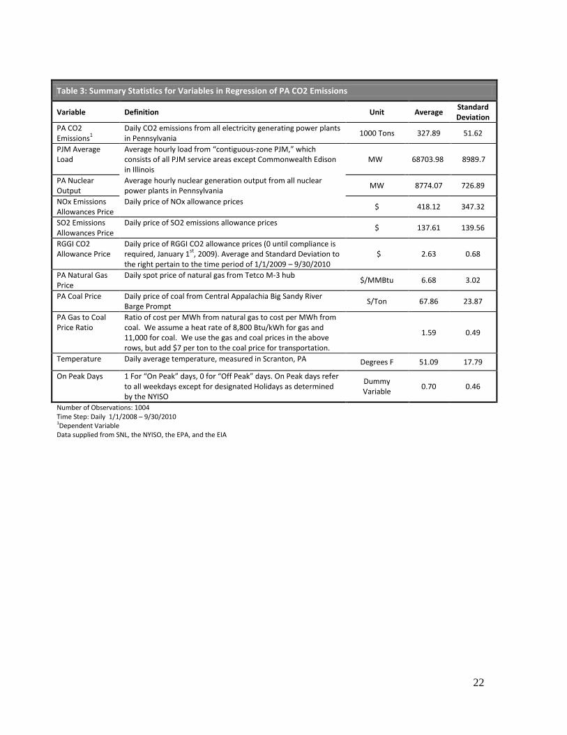
Table 3: Summary Statistics for Variables in Regression of PA CO2 Emissions

Variable Definition Unit Average Standard Deviation

PA CO2 Emissions

1 Daily CO2 emissions from all electricity generating power plants in Pennsylvania

1000 Tons 327.89 51.62

PJM Average Load

Average hourly load from “contiguous-zone PJM,” which consists of all PJM service areas except Commonwealth Edison in Illinois

MW 68703.98 8989.7

PA Nuclear Output

Average hourly nuclear generation output from all nuclear power plants in Pennsylvania

MW 8774.07 726.89

NOx Emissions Allowances Price

Daily price of NOx allowance prices $ 418.12 347.32

SO2 Emissions Allowances Price

Daily price of SO2 emissions allowance prices $ 137.61 139.56

RGGI CO2 Allowance Price

Daily price of RGGI CO2 allowance prices (0 until compliance is required, January 1

st, 2009). Average and Standard Deviation to

the right pertain to the time period of 1/1/2009 – 9/30/2010 $ 2.63 0.68

PA Natural Gas Price

Daily spot price of natural gas from Tetco M-3 hub $/MMBtu 6.68 3.02

PA Coal Price Daily price of coal from Central Appalachia Big Sandy River Barge Prompt

S/Ton 67.86 23.87

PA Gas to Coal Price Ratio

Ratio of cost per MWh from natural gas to cost per MWh from coal. We assume a heat rate of 8,800 Btu/kWh for gas and 11,000 for coal. We use the gas and coal prices in the above rows, but add $7 per ton to the coal price for transportation.

1.59 0.49

Temperature Daily average temperature, measured in Scranton, PA Degrees F 51.09 17.79

On Peak Days 1 For “On Peak” days, 0 for “Off Peak” days. On Peak days refer to all weekdays except for designated Holidays as determined by the NYISO

Dummy Variable

0.70 0.46

Number of Observations: 1004 Time Step: Daily 1/1/2008 – 9/30/2010 1Dependent Variable Data supplied from SNL, the NYISO, the EPA, and the EIA

23

Table 4: Regression of PA CO2 emissions with Cochrane-Orcutt

transformation

Regressor (1) (2) (3) (4) (5) (6)

PJM Average Load 1.224***

(0.123)

1.220***

(0.123)

1.215***

(0.123)

1.207***

(0.122)

1.213***

(0.122)

1.206***

(0.122)

PJM Average Load2 -0.455*** (0.119)

-0.453*** (0.119)

-0.447*** (0.119)

-0.435*** (0.117)

-0.446*** (0.118)

-0.434*** (0.117)

RGGI CO2 Allowance Price 0.00814

(0.0538)

0.00897

(0.0540)

0.0238

(0.0515)

0.0197

(0.0510)

-0.0113

(0.0466)

-0.0135

(0.0462)

PA Nuclear Output -0.0464*

(0.0198)

-0.0467*

(0.0190)

-0.0465*

(0.0198)

-0.0467*

(0.0198)

-0.0455*

(0.0198)

-0.0456*

(0.0198)

NOx Price -0.130 (0.0686)

-0.132 (0.0689)

-0.159** (0.0602)

-0.154** (0.0609)

-0.108* (0.0535)

-0.106* (0.0529)

SO2 Price -0.0492

(0.0622)

-0.0525

(0.0623)

PA Natural Gas Price 0.0248 (0.0316)

0.0251 (0.0316)

0.0204 (0.0310)

PA Coal Price 0.0752

(0.0623)

0.0794

(0.0626)

0.0873

(0.0621)

0.0956

(0.0609)

Natural Gas to Coal Price Ratio

0.0125 (0.0189)

Temperature 0.0128

(0.0198)

On Peak Day 0.104***

(0.0191)

0.104***

(0.0190)

0.105***

(0.0190)

0.103***

(0.0188)

0.105***

(0.0190)

0.102***

(0.0188)

Intercept -0.104* (0.0482)

-0.104* (0.0486)

-0.105* (0.0491)

-0.103* (0.0486)

-0.108 (0.0509)

-0.106* (0.0503)

Adjusted R2 .7964 .7965 .7965 .7967 .7960 .7962

N 1002 1002 1002 1002 1002 1002

Rounded standard errors are listed in parentheses under the coefficients.

* p<0.05, ** p<0.01, *** p<0.001

24

Appendix 2 – Additional Detail About Methods

Models were estimated in STATA, an advanced statistical analysis package. Explanatory

variables, to be used to attempt to explain the dependent variables of Pennsylvania CO2

emissions and Pennsylvania-to-New York power flows, were selected based on previous

studies, first principles, data availability, experience of the authors and input from

others at the NYISO.

Results from initial ordinary least squares (OLS) regression analysis indicated strong

serial correlation. This occurs when the prediction error in consecutive time periods are

correlated. The presence of serial correlation was determined by graphs of the residuals

over time which indicated positive serial correlation and by statistical tests. Durbin-

Watson D-statistics were approximately 0.6. Breusch-Godfrey tests for first-order serial

correlation were statistically significant. Partial autocorrelograms of the residuals

indicated first order correlation as the observations in the first time period were highly

significant followed by insignificance in later time periods.

Initial regressions were analyzed for other structural defects. Cook and Weisberg tests

for heteroscedasticity were insignificant, indicating no heteroscedasticity problems. A

Phillips-Perron unit root test was performed to test for stationarity of the dependent

variables. Results were significant, leading to a rejection of the null hypothesis of a unit

root, and support for the alternative hypothesis that the dependent variables could be

treated as stationary during the timespan of our data.

To correct for first order serial correlation, models were estimated using generalized

least squares (GLS) methods. The Cochrane-Orcutt transformation was used to

iteratively estimate the coefficient of first order serial correlation, ρ (“rho”). The

estimated ρ is the value of the regression coefficient that would result from a regression

of each error term on the error term from the preceding time period. Since the exact

value of this regression coefficient is unkown, the Cochrane-Orcutt transformation

iteratively estimates its value and then corrects for the serial correlation using the

estimated ρ.

Results of the transformed model were tested to determine the effectiveness of the

correction. Durbin-Watson D-statistics were close to two indicating little or no

remaining serial correlation. Breusch-Godfrey tests for first order serial correlation were

insignificant. Finally, the error term from the estimate of the dependent variable was

put into an AR(1) ARIMA model in which it was regressed against the lag of itself. A

25

Portmanteau white noise test failed to reject the hypothesis that the resulting residuals

were white noise indicating that serial correlation was corrected.

Multicollinearity was determined not to be a problem. The variance inflation factors

(VIF) for all explanatory variables were under 5 in each model, except in the models of

scheduled flows, in which New York natural gas price had a VIF just above 7. GLS

regressions run on the New York natural gas price with individual explanatory variables

result in no relationships with p-values below 0.2.

Visual inspection of the data indicated non-linear relationships between scheduled flow

and the NOx allowance price, and between Pennsylvania CO2 emissions and PJM load.

In each case, including the square of the explanatory variable in question as an

additional explanatory variable produced a higher adjusted r-squared than omitting the

square or including both the square and the cube.

Relationships of each dependent variable with other explanatory variables were also

tested by trying non-linear transformations of the explanatory variables such as

squaring, logging, and linear or cubic splines. For the variables other than the two

mentioned in the preceding paragraph, linear relationships were judged suitable, as

determined by changes in adjusted r-squared values, p-values of the variables, and F-

tests for joint significance.

26

REFERENCES

EIPC (2010). Eastern Interconnection Planning Collaborative. “Coordination of MRN-

NEEM Modeling andHigh Level Transmission Analysis in Task 5--December 30

Revision of the presentationat Macro Future Workshop November 8-9,2010”

Accessed January 7, 2010 at

http://www.eipconline.com/uploads/Transmission_in_MRN-

NEEM_New_FINAL_12-30-10.pdf.

ICF Consulting (2006a). Assumption Development Document: Regional Greenhouse Gas

Initiative Analysis. Accessed 1/5/2011 at

http://www.rggi.org/docs/ipm_assumptions_2_10_05.ppt

ICF Consulting (2006b). RGGI Preliminary Electricity Sector Modeling Results: Phase

III RGGI Reference and Package Scenario. Accessed 1/5/2011 at

http://www.rggi.org/docs/ipm_modeling_results_10.11.06.ppt

RGGI Inc. Emissions Leakage Multi-State Staff Working Group (2007a). Potential

Emissions Leakage and the Regional Greenhouse Gas Initiative (RGGI): Evaluating

Market Dynamics, Monitoring Options, and Possible Mitigation Mechanisms

Accessed at http://rggi.org/docs/il_report_final_3_14_07.pdf

RGGI Inc. (2007b). Overview of RGGI CO2 Budget Trading Program. October 2007.

Accessed February 22, 2011 at http://rggi.org/docs/program_summary_10_07.pdf.

Monitoring Analytics, LLC (2010). State of the Market Report for PJM 2009. Accessed

12/21/10 at

http://www.monitoringanalytics.com/reports/PJM_State_of_the_Market/2009/200

9-som-pjm-volume2-sec1.pdf

New York State Energy Research and Development Authority (NYSERDA). (2010).

Relative Effects of Various Factors on RGGI Electricity Sector CO2 Emissions: 2009

Compared to 2005. RGGI, Inc. Prepared by NYSERDA for RGGI, Inc. Accessed

12/20/10 at

http://www.rggi.org/docs/Retrospective_Analysis_Draft_White_Paper.pdf

Palmer, K. (2006, October). Insights from Modeling of the RGGI CO2 Cap and Trade

Program [Presentation Slides].

Paltsev, S.V. (2001). The Kyoto Protocol: Regional and Sectoral Contributions to the

Carbon Leakage. The Energy Journal, 22(4), 53-79.

27

Potomac Economics (2009). RGGI Auction 3 on March 18, 2009 Memorandum. Accessed

12/20/10 at http://www.rggi.org/docs/Auction_3_MM_Report.pdf

Potomac Economics (2010). Market Monitor Report for Auction 10. Accessed 12/20/10

at http://www.rggi.org/docs/Auction_10_Market_Monitor_Report.pdf

Public Service Electric and Gas Company (2009). Leakage SRT-114 Update with Exhibits.

BPU Docket No EM09010035.

RGGI Emissions Leakage Multi-State Staff Working Group (2008). Potential Emissions

Leakage and the Regional Greenhouse Gas Initiative (RGGI). Accessed 12/20/10 at

http://www.rggi.org/docs/20080331leakage.pdf

Shawhan, D.L., Mitarotonda, D.C., Zimmerman, R.D., & Taber, J.T. (2010) An Advanced

Method of Predicting Power-Sector Environmental Policy Outcomes. Mimeo.