an empirical model of mobile advertising platforms

AN EMPIRICAL MODEL OF MOBILE ADVERTISINGPLATFORMS

KHAI X. CHIONG AND RICHARD Y. CHEN

Abstract. We study a new online advertising platform, created specificallyfor mobile app-to-app advertising. Both advertisers and publishers are mobileapplications (apps). Advertisers seek to acquire new users for their mobileapps, while publishers seek to monetize their apps. Our data come from theintermediary who operates this two-sided platform, and who uses a central-ized market-clearing mechanism to meet the demand with the supply of users’in-app impressions. Notably in this mechanism, advertisers bid for impres-sions, but only pay when impressions are won and when ads lead to useracquisitions (pay-per-install). We develop a model for the advertiser’s optimalbidding problem, and use observed bids to recover the advertiser’s valuationor willingness-to-pay for a new user.

We find certain segments of this market to be severely uncompetitive, re-sulting in large bid-shading, and lost profit for the intermediary and publishers.Using the estimated model, we discuss how the intermediary can make the plat-form more competitive. Interestingly, we also find that how much a user spendson in-app purchases contributed to only about 10% of the average advertiser’svaluation for that user. We argue that this relatively large unobserved valua-tion partly stems from advertisers’ resale motives: after acquiring users andselling in-app purchases to them, an advertiser then has the option to resellthese users by becoming a publisher, selling these users’ impressions to otheradvertisers. Thereby, the advertiser participates in both sides of the market asan advertiser and a publisher.

1. Introduction

The Internet and smart mobile devices are transforming how consumers receiveinformation of new products. Digital advertising, which consists of online andmobile advertising among others, has become an increasingly important part ofmany businesses’ marketing channels. In 2015, businesses’ spending on digital

Date: October 2016.Khai Chiong (corresponding author): USC Dornsife INET, Department of Economics, Uni-

versity of Southern California, [email protected] Chen: OpenAI, [email protected]. Acknowledgements are at the end of

the document. All errors remain our own.

1

mailto:[email protected]

[email protected]

2 KHAI X. CHIONG AND RICHARD Y. CHEN

advertising1 increased by 17.2% to $160 billion. In fact, 2017 is widely projectedto be the tipping point when businesses spend more on digital advertising thantraditional media advertising such as TV and print.2 Driving this stunning rise ismobile advertising. Mobile devices have now firmly replaced desktop and laptopcomputers as the primary means for individuals to access the Internet, and inmany emerging economies, they are the only means. According to Google, moresearches now take place on mobile devices than on computers in 10 countriesincluding the U.S. and Japan. Moreover in the U.S., spending on mobile adver-tising amounts to $31.59 billions in 2015, which is more than half of the total$59.61 spending on all digital advertising.3

In this paper, we introduce a new online advertising platform, which has beenspecifically created for the purpose of mobile app-to-app advertising. In this two-sided platform, both advertisers and publishers are mobile apps (applications).For instance, we could have Uber advertises on Instagram, the Starbucks mo-bile app advertises on the Waze app (GPS-based navigational app), or a mobilegaming app advertises on another gaming app. Mobile apps have become themain interface between consumers and firms within mobile devices. On the con-sumer’s side, users prefer to install a myriad of mobile apps for their differentneeds than to use a mobile web browser.4 Individual apps are able to providebetter user experience and personalization.5 On the firm’s side, firms includingtraditional retailers, are facing a growing need to develop and market their pres-ences in mobile devices as mobile apps, which act as a gateway to branding andpurchases.

In this new online advertising platform, advertisers and publishers participate ina new bidding mechanism whereby advertisers set bids which are promises-to-pay when (i) advertisers win the slot to show ads, and (ii) users take a certainaction after ads. This is known as a CPA (cost-per-action) bid. Particularlyin our app-to-app environment, this user’s action is specifically defined as theinstallation of the advertiser’s app. That is, advertisers bid for users’ impressions,

1Digital advertising includes all advertising (online and offline) that appears on digital mediadevices, which is defined by being interactive, personalized, or Internet-connected, such asdesktop, laptop computers, mobile phones, tablets, gaming consoles.

2New York Times (December 7, 2015). Digital Ad Spending Expected to Soon Surpass TV.The Economist (March 26, 2016). Invisible ads, phantom readers.

3eMarketer (March 8, 2016). Digital Ad Spending to Surpass TV Next Year.4ComScore: the average users of mobile devices in the U.S. spend 86% of their time on

mobile apps, as opposed to 14% on mobile web browsers.5App developers can maximize precious screen real estate by getting rid of navigation bars

imposed by the web browsers. They can access phone features such as push-notification, camera,GPS, physical sensors. Once installed, apps also work faster than their web-counterparts.

AN EMPIRICAL MODEL OF MOBILE ADVERTISING PLATFORMS 3

but only pay this bid to the publisher in the event that their ads lead to auser acquisition or install. This platform mechanism is highly attractive to theadvertisers, who only need to pay per user’s install. It aligns with the objective ofthe app developers who operate on the “freemium” business model (see Lee et al.(2015)), which seeks to acquire as many new users as possible. With this newbidding mechanism, publishers are now more accountable for ad effectiveness, asthey would otherwise be selling impressions for free if ads do not lead to a desireduser’s response. CPI (cost-per-install) advertising has seen stunning rise in thepast few years. Businesses’ spending on CPI campaigns has increased by 80%from 2014 to 2015, and accounted for 10.3% of total mobile advertising spend in2015.6

Another feature of this platform that we exploit is that mobile advertisers havethe capability to track the behavior of users post viewing of ads. Advertisersuse these user-tracking data to actively inform their valuations and to optimizebids. For instance, advertisers know how much different types of acquired usersspend on in-app purchases, which are products offered by the mobile apps. Thesetracking capabilities contrast with traditional advertising channels such as TV,newspapers, and roadside billboards, which do not allow advertisers to under-stand users’ behavior after viewing an ad.7 Tracking user’s spending on in-apppurchases is an important task due to the “freemium” business model adoptedby a vast majority of mobile apps – installing the apps is free, monetization isachieved by a small fraction of users paying for additional premium content withinthe app (which includes monthly subscriptions and in-game currency).

The contribution of our paper is two-fold. Firstly, we take the managerial per-spective that the intermediary is our client, and we seek to optimize the platformdesign in order to increase the intermediary’s revenue. Secondly, we advanceour understanding of the behavior of advertisers in the context where they canalso participate in the other side of the market as publishers. To achieve this,we develop a model for the advertiser’s optimal bidding problem. We then useobserved bids to recover the advertiser’s valuation or willingness-to-pay for a newuser. Our data come from the intermediary, which is the entity who operates thistwo-sided platform.

Knowing the advertiser’s valuation allows us to quantify the margin of strategicbid-shading – the difference between valuation and observed bids, or in anotherwords, how much profit the intermediary and publishers are losing as a result

6eMarketer (December, 2015). Mobile Advertising and Marketing Trends Roundup7Another important feature of digital advertising is its capability to target users with much

higher precision (Goldfarb (2014))


of uncompetitive bidding among the advertisers. We find that certain segmentsof the market are severely uncompetitive. We discuss several policies the inter-mediary can pursue to increase competition among advertisers. We also use theestimated model to evaluate the counterfactual effectiveness of these policies. Forinstance, we show that in some cases, it is desirable to introduce some inaccu-racy in the score. Specifically, it is sometimes desirable to boost and increase thescores of some uncompetitive and low-quality advertisers. On one hand, scoreboosting introduces inaccuracy and mismatch in the matching so that there arenow fewer user acquisitions, but on the other hand, it stimulates more aggressivebidding by advertisers. Overall, score-boosting can increase the revenue of theintermediary.

Our numerical result: the estimated valuation for a new user is $12.69 for theaverage advertiser. For the median advertiser, it is $8.55. The interquartile rangeis [$5.10, $15.53]. By comparison, the advertisers ended up paying significantlyless to acquire these users: the average winning bid is $4.04, and the median at$3.50. This leads to a large margin (difference between willingness-to-pay and theprice paid) that ranges from $1.87 to $10.52 in the interquartile range. Our resultstrongly suggests that certain segments of the market are severely uncompetitive,where advertisers can shade their bids well below their valuations, and still wina large number of impressions. This leads to lost profits for the publishers andintermediary.

Further, we decompose the valuation for a new user into two parts: the firstpart is the sales revenue from in-app purchases made by the acquired user; thesecond part is the advertiser’s unobserved valuation, which represents the residualvalue that the acquired user brings to the advertiser. The first part is observedusing data that track user’s spending on in-app purchases after acquisition.8 In-app purchases are products offered by the app developer within the app, whichtake the form of additional content, services or subscriptions within the app. Inour sample, the 4,973,931 users that were acquired in the span of 47 days, havespent a total of $679,470 on in-app purchases. Methodologically, the advertiser’svaluation is partially observed, and we exploit the information in this observedcomponent to better estimate the overall valuation.

However we find that users’ spending account for about 9% of an average adver-tiser’s overall valuation. This is puzzling given the importance of users’ in-apppurchases.9 We offer an explanation for what drives the advertiser’s valuation

8Which is routinely collected by advertising intermediaries, where they then inform adver-tisers of their Return on Investments (ROI) of advertising.

9One popular mobile gaming app, Clash of Clans, generates $4 million a day from in-apppurchases (the app developer was recently acquired for $8.6 billion by Tencent).


for user acquisitions: due to the app-to-app advertising nature of our platform,an app developer can readily participate in both sides of the market, as bothan advertiser and a publisher. This introduces resale motive which partlydrives up the advertisers’ valuations for a new user.

More concretely, the advertiser perceives a user as a durable good, wherebya user generates a stream of diminishing monetary benefits in terms of in-apppurchases. Now the advertiser then has the option to resell a user by selling itsimpression and attention to other advertisers. By reselling the attention of theuser, the user would potentially be drawn away to other apps (due to the scoringprocedure used by the platform mechanism, the ads that are shown to this user areoften competing apps that are closely relevant to the user). The crucial questionthis naturally leads to is, how then should firms optimally predict and measurethe lifetime value of their customers, given this resale option? To our knowledge,this goes beyond the standard models of customer lifetime valuation.

The estimation procedure is based on the Generalized Method of Moments (GMM),where the moment conditions provide a link between (i) observed bids; (ii) ob-served valuation due to users’ spending; (iii) unobserved valuations. Intuitively,we use a profit-maximization framework to derive advertisers’ first-order optimal-ity conditions trading off the expected benefit and cost of higher bids. Althoughthe estimation procedure is frequentist in nature, our model also lends itself nat-urally to a full-information likelihood approach, which can be estimated usingBayesian methods.

1.1. Related literature

First, our paper is related to the vast literature of digital advertising. Mobileadvertising includes keyword search advertising that takes place in mobile devices.Theoretical papers that analyse search advertising are Amaldoss et al. (2015);Shin (2015), while empirical papers in this area include Athey and Nekipelov(2010); Hsieh et al. (2014); Jeziorski and Moorthy (2016); Rutz and Bucklin(2011); Yang and Ghose (2010); Yao and Mela (2011)). Display advertising suchas banner advertising (Andrews et al. (2015); Bruce et al. (2016); Johnson (2013);Manchanda et al. (2006)) has been studied extensively in the context of webbrowsers on desktop or laptop computers. Display advertising can also occurin mobile devices (see Bart et al. (2014) who study mobile display advertising(MDA)).

Our paper studies a growing form of mobile advertising called app-to-app adver-tising, where companies seek to promote their mobile apps within other mobileapps. The fast-rising prominence of the mobile app economy has been noted


and studied in a recent paper by Ghose and Han (2014), which uses a structuralmodel to estimate the demand for mobile apps.

The intermediary we study in this paper is an example of an online advertisingplatform or network, which provides a common marketplace for advertisers andpublishers to buy and sell impressions (see Sriram et al. (2015) for a survey ofrecent work related to advertising platforms). In a novel paper, Wu (2015) studiesan online advertising platform which uses a decentralized matching mechanism,as opposed to the centralized mechanism here. An important role of an onlineadvertising platform is the ability to facilitate the delivery of targeted ads tousers (Goldfarb and Tucker (2011); Iyer et al. (2005); Lambrecht and Tucker(2013); Sayedi et al. (2014); Zhang and Katona (2012)). In mobile advertising,targeting can be achieved with even more degrees of freedom, due to built-inGPS sensors in mobile devices (see Andrews et al. (2014); Fong et al. (2015);Grewal et al. (2016); Luo et al. (2013); Zubcsek et al. (2015)). More generally,mobile advertising goes beyond mobile app-to-app advertising in this paper. Italso includes firms using SMS to send promotional messages (see Andrews et al.(2016); Shankar and Balasubramanian (2009) for comprehensive surveys of mobilemarketing).

The CPI (cost-per-install) advertising considered in this paper is a type ofperformance-based or CPA (cost-per-action) advertising which includes the pop-ular CPC (cost-per-click). The CPC pricing scheme where advertisers pay perclicks have received much attention in the literature (Agarwal et al. (2009); As-demir et al. (2012); Ghose and Yang (2009); Hu et al. (2015); Liu and Viswanathan(2014); Zhu and Wilbur (2011)). Another common pricing scheme is CPM whereadvertisers pay per impression. The CPI advertising we considered here is morerecent and attributed to the recent rise of the mobile app economy and app-to-app advertising. The objective of a CPI advertising campaign is user acquisi-tion.

Another related area is modeling customers’ lifetime value. These papers arenormative, i.e. prescribing how to measure CLV, while our paper here is descrip-tive in nature, i.e. asking what advertisers are doing to form their valuations.For primers on modeling CLV, we refer to Fader and Hardie (2005); Fader et al.(2005); Gupta et al. (2006); Schmittlein et al. (1987). Here, another importantpaper is Chan et al. (2011), which estimate the lifetime value for a firm’s cus-tomers acquired through sponsored search advertising (cost-per-click campaigns)on Google based on the Pareto/NBD model.

Also noteworthy is the literature on measuring the returns on investment (ROI)of online advertising. The valuation of the advertiser for a new user is strongly


related to how much returns they expect to receive from advertising. Lewisand Rao (2015) highlighted the challenges for advertisers to evaluate the ROIfrom impression-based (CPM) advertising campaigns. A related paper on causaleffectiveness and ROI of sponsored search advertising is Blake et al. (2015).

2. Industry Background

A mobile app is a computer program designed to run on mobile devices suchas smartphones and tablet computers. The mobile apps industry started withthe introduction of the iPhone and Apple’s app store in 2008. App developersmarket their products through distribution platforms called app stores (Appleapp store and the Google Play are the two largest), which takes a 30% cut outof the developer’s revenue.

By far the overwhelming fraction of mobile apps have adopted the ‘freemium’business model,10 such that the users install the app for free and are given theoption to make in-app purchases (see also Lee et al. (2015)). A well-knownsuccess stories of the freemium model is the mobile game Clash of Clans, whichgenerates $4 million a day in revenue, just from in-app purchases. Supercell, itsapp developer, posted $2.4 billion in revenue in 2015, and was recently acquiredby the Chinese internet giant, Tencent, for $8.6 billion. This transaction is theseventh largest Chinese overseas acquisition on record.

The genres of mobile apps include photography (Instagram), social networking,health & fitness, shopping, travel & navigation (Uber), news, books, utilities,music. By far the most prominent is the gaming genre – global revenue frommobile games is on track to rise 21% to about $37 billion this year.11

A primary concern of mobile app developer is marketing. While mobile appssuch as Instagram are worth $1 billion, many mobile apps are not worth much.In 2015, Apple announced that there were over 1.5 million apps in the Appleapp store, and over 100 billion apps had been downloaded.12 Two stylized factsstand out: the large number of products available on the app store, and the large

10In 2014, freemium app revenue now accounts for 98% of worldwide revenueon Google Play, with Japan, U.S. and South Korea users contributing the most.http://blog.appannie.com/google-io-special-report-launch-2014/

11Tencent President Martin Lau said “We are very bullish on the [mobilegames] market” http://www.wsj.com/articles/tencent-agrees-to-acquire-clash-of-clans-maker-supercell-1466493612

12http://www.statista.com/statistics/263794/number-of-downloads-from-the-apple-app-store/


number of potential users dispersed worldwide. Marketing and advertising theirproducts have become essential for mobile app developers.

Recognizing this challenge, several platforms have begun to fill this niche in thelast several years. The San Francisco-based start-up from which our data areobtained exists in such a niche.

2.1. How the platform works

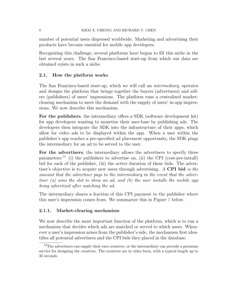
The San Francisco-based start-up, which we will call an intermediary, operatesand designs the platform that brings together the buyers (advertisers) and sell-ers (publishers) of users’ impressions. The platform runs a centralized market-clearing mechanism to meet the demand with the supply of users’ in-app impres-sions. We now describe this mechanism.

For the publishers, the intermediary offers a SDK (software development kit)for app developers wanting to monetize their user-base by publishing ads. Thedevelopers then integrate the SDK into the infrastructure of their apps, whichallow for video ads to be displayed within the app. When a user within thepublisher’s app reaches a pre-specified ad placement opportunity, the SDK pingsthe intermediary for an ad to be served to the user.

For the advertisers, the intermediary allows the advertisers to specify threeparameters:13 (i) the publishers to advertise on, (ii) the CPI (cost-per-install)bid for each of the publisher, (iii) the active duration of these bids. The adver-tiser’s objective is to acquire new users through advertising. A CPI bid is theamount that the advertiser pays to the intermediary in the event that the adver-tiser (a) wins the slot to show an ad, and (b) the user installs the mobile appbeing advertised after watching the ad.

The intermediary shares a fraction of this CPI payment to the publisher wherethis user’s impression comes from. We summarize this in Figure 1 below.

2.1.1. Market-clearing mechanism

We now describe the most important function of the platform, which is to run amechanism that decides which ads are matched or served to which users. When-ever a user’s impression arises from the publisher’s side, the mechanism first iden-tifies all potential advertisers and the CPI bids they placed in the database.

13The advertisers can supply their own creatives, or the intermediary can provide a premiumservice for designing the creatives. The creatives are in video form, with a typical length up to35 seconds.


IntermediaryAdvertisers(Mobile app developers)

Publishers(Mobile app developers)

Users Users

CPI bids Revenue share

Users

Figure 1. Overview of how the platform works

Next, the mechanism assigns a score to each ad based on the following formula:CPI×Score, where Score is the estimated probability that the user would installthe advertised app conditional on viewing the ad. It is calculated by plugging inthe user and advertiser’s attributes into a prediction model.

The mechanism then selects the ad with the highest score-weighted CPI bid asthe winner of that user’s impression. This ad will be shown to the user. Afterthe user watches the ad, he or she can click and proceed to the advertiser’s pagein the App Store. If the user installs the app, we say the user is acquired by theadvertiser. If the user does not install, the advertiser is not charged, otherwise,the advertiser pays the CPI bid to the intermediary (who passes a fraction of thisrevenue to the publisher).

The score-weighted CPI bid associated with a pair of user and ad is just theexpected amount that the advertiser pays for that user’s impression. Intuitivelythen, for each user’s impression that arises, the mechanism selects the advertiserwith the highest expected payment to be the winner.

2.2. Advertiser’s information set

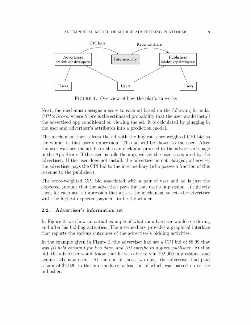
In Figure 2, we show an actual example of what an advertiser would see duringand after his bidding activities. The intermediary provides a graphical interfacethat reports the various outcomes of the advertiser’s bidding activities.

In the example given in Figure 2, the advertiser had set a CPI bid of $8.99 thatwas (i) held constant for two days, and (ii) specific to a given publisher. At thatbid, the advertiser would know that he was able to win 192,000 impressions, andacquire 447 new users. At the end of those two days, the advertiser had paida sum of $4,020 to the intermediary, a fraction of which was passed on to thepublisher.


Figure 2. Advertiser’s information set: what do advertisers see?

3. Model

Consider a setup between one advertiser and one publisher. In this section,we propose a model for how the advertiser forms his bid for that publisher,conditional on choosing to bid on that publisher.


The advertiser has a valuation v for the user. This valuation is a random vari-able, to reflect the fact that the advertiser is bidding to acquire a distributionof users who benefit the advertiser heterogeneously. Now the advertiser knowsthe probability distribution of v, but it is not known to us. Ultimately, we wantto learn about v, which is also known as the advertiser’s willingness-to-pay for anew user.14

When the advertiser submits a bid of p, he expects to acquire Q(p) number ofusers from the publisher. Now Q(·) is a random function, i.e. Q(p) is a randomvariable whose probability distribution is parameterized by p. The expected profitof the advertiser when he bids p is:

U(p) = E[(v − p)Q(p)](1)

The expectation in Equation (1) is taken over the joint probability density of(v,Q(p)). We will refer to Q(p) as the supply curve. We refer to Section 3.2 fora detailed comparison with the standard auction setup.

3.1. Specifying the supply curve

We now specify Q(p), which is the advertiser’s belief about the number of users hewill successfully acquire at different levels of bid p. In formulating Q(p), we modelclosely how the advertiser’s bids is translated into numbers of user acquisitions.See Section 2.1.

Q(p) = F (s · p)N · χ · s(2)

Now, the advertiser believes that the score-weighted bids of each of his com-petitor is distributed independently with the cumulative density function F (·).Therefore, the advertiser believes that he will win each impression with proba-bility F (s · p)N where N is the number of competing bidders, and s is the qualityscore associated with the advertiser. For a given user that arises from the pub-lisher, the intermediary computes a quality score that equals to the estimatedprobability that the user would install after watching the advertiser’s ad. Thisscore s is a random variable (since different users within the publisher would havedifferent scores). For simplicity, we will first take s to be the average score of

14See Chan et al. (2007), where they define WTP as the maximum amount a bidder is willingto bid for an item such that she is indifferent between winning the item at this bid and notwinning.


the advertiser specific to the publisher. In the empirical section, we show how torelax this assumption in the estimation.

χ is the random variable representing the advertiser’s belief about the total num-ber of impressions that would be supplied by the publisher. Therefore F (s ·p)N ·χis the number of impressions that the advertiser expects to win at bid p. Notethat χ and s do not depend on p. Although the number of competing biddersN is fixed, in Section 4.7, we allow it to be a random variable to reflect entryuncertainty.

Finally, since the quality score s is the probability that a user would install afterbeing shown the advertiser’s app, F (s ·p)N ·χ · s is then the number of users thatthe advertiser expects to acquire at bid p.

For ease of notation, we will introduce the following:

α(p) ≡ F (s · p)N(3)

That is, α(p) is the probability that the advertiser expects to win an impressionat bid p.

Proposition 1. Suppose that the advertiser’s expected profit is given by Equation1. Then the optimal bid p∗ satisfies:

α(p∗)/p∗

∂α(p)∂p

∣∣∣p∗

=1

p∗E[vχ]

E[χ]− 1(4)

Plugging in α(p) = F (s ·p), where F (·) is the advertiser’s belief about the CDF ofthe adjusted CPI bids of other competing bidders, and f(·) is the correspondingPDF, we then have:

F (sp∗)

sp∗Nf(sp∗)=

1

p∗E[vχ]

E[χ]− 1(5)

We relegate all proofs to the appendix. The LHS of Equation 4 is the inverse ofthe elasticity of α(p) with respect to p evaluated at p∗.

Proposition 2. When F (·) is the CDF of the lognormal distribution, thereis a unique optimal bid p∗ that satisfies Equation 5. In particular, sufficient


conditions for the optimal bid p∗ satisfying Equation 5 to be unique are: (i)

limz→0+F (z)zf(z)

= 0, and (ii) F (z)zf(z)

is strictly monotonically increasing in z. Both of

these conditions are satisfied when F (·) is the CDF of the lognormal distribution.

In particular, when F (·) is the CDF of the lognormal distribution with parameter(µ, σ), that is, the random variable X drawn from the distribution F is such thatlogX is distributed N(µ, σ), then

√2π

Nσe

(µ−log(sp))2

2σ2 Φ

(log(sp)− µ

σ

)=

1

p

E[vχ]

E[χ]− 1(6)

where Φ(·) is the CDF of the standard Gaussian. In the appendix, we show thatthe LHS of Equation 27 is strictly monotonically increasing in p, and convergesto zero as p→ 0+.

Proposition 3 below states the factors that determine the advertiser’s optimalbid. Intuitively, bidding higher increases the advertiser’s chance of winning, butthe advertiser also ends up paying more if he does win. The optimal bid dependson this trade-off.

Proposition 3. Assume that the conditions in Proposition 2 hold. The adver-tiser’s optimal CPI bid p∗ is larger when:

(1) E[vχ]E[χ] is larger;

(2) N , the number of competing bidders is larger;

(3) F (x)xf(x)

is weakly smaller for all x > 0 and strictly smaller for some x >

0, where f(·) and F (·) are the probability and cumulative distributionfunctions associated with the advertiser’s belief about the score-weightedCPI bids of other competing bidders.

In another words, the slope of the function F (x)xf(x)

determines how competitive

the market is. When the function F (x)xf(x)

is steep, the market is less competitive.

Moreover consider F (·) and f(·) such that F (·) is a first-order stochastic dominantshift of F (·). Then it follows that F (x) ≥ F (x) at all x > 0 and F (x) > F (x)for some x. A first-order stochastic dominant shift can be achieved by takinga mass of bidders and increasing their score weighted CPI bids, holding all elseconstant. If this first-order stochastic dominant shift is large enough such thatF (x)xf(x)

is weakly larger than F (x)

xf(x)for all x and strictly larger for some x, then the

advertiser would increase its’ bid.


To give an example, we can verify that if F is the CDF of the triangular distri-bution with support [0, 1] and mode of 0.25, and F is the CDF of the triangular

distribution with support [0, 1] and mode of 0.75, then it is true that F (x)xf(x)

≥ F (x)

xf(x)

for all x ∈ [0, 1], and F (x)xf(x)

> F (x)

xf(x)for all x ∈ [0.25, 1]. However, F first-order

stochastically dominates F does not guarantee that F (x)xf(x)

≥ F (x)

xf(x).

3.2. Remark: comparison with standard auction setups

Our setup differs from the standard auction setups due to the kind of informationthat is available to the advertisers in our platform (see Section 2.2). Notably, ouradvertisers can only set a single bid for the whole publisher – this bid applies toall users in that publisher. Moreover, this bid is held constant over a given timeperiod.

Therefore, our advertisers do not bid for each user’s impression, but bid for adistribution of heterogeneous impressions. At the time the bid is placed, thebidder’s valuation is a random variable, as opposed to a realized, fixed number.To form the optimal bid, the bidder has to first integrate out his belief about therandomness in this valuation and obtains the expected profit equation in 1.

In comparison, in an online ad exchange, advertisers are able to bid for eachimpression in real-time, programmatically. The standard auction setup thenapplies to such online ad exchanges because we can treat each impression ashaving a known value to the advertiser at the time he forms his bid.

The final distinction here is that bidders do not know the identities of competingbidders. In contrast, in a keyword search advertising, the bidder can search for thekeyword and find out who eventually won the top slots. The intermediary ensuresmutual anonymity between participating advertisers (see Figure 2). Therefore,we will later take a mean-field approximation approach (Weintraub et al. (2005))to modeling strategic interaction among bidders – by assuming that agents arebest-responding to the correct distribution of opponents’ bids, instead of best-responding to opponents’ bidding strategies.

4. The Econometric Model

In this section, we develop an econometric model based on the previous theoreticalmodel. The goal is to recover the advertiser’s valuation v using observed bids.In particular, v is a random variable, and we provide an estimator for E[v]. In


the empirical application, we will estimate one such valuation parameter for 216different advertiser-publisher pairs, obtaining 216 parameter estimates.

4.1. The econometrician’s uncertainty

In our previous theoretical model, there is no econometrician’s uncertainty. Recallthat there is then a single optimal bid that is consistent with the model. As such,we are not able to rationalize the data where observed bids could be changingover time. Therefore we need to incorporate the econometrician’s uncertainty inorder to fit the data to our model.

Before the advertiser sets the bid, he observes a shock to the supply curve ε. Theadvertiser then sets his bid to maximize the expected profit equation below:

U(p; ε) = E[(v − p)(Q(p) + ε)](7)

We do not observe this shock. This represents the econometrician’s uncertainty.Moreover ε is unanticipated by the advertiser, as such, the expectation above isonly taken with respect to the joint distribution of (v,Q(p)).

4.2. Partially observed valuation

Now for the purpose of estimation, we want to incorporate additional informationthat we (the econometrician and the intermediary) has about the advertiser’s val-uation. We do this by formulating the valuation as being partially observed.

Specifically, let v = x + ξ, where x is the random variable representing thebelief about how much a user acquired from the publisher would spend on in-app purchases in the first 14 days after acquisition; ξ is the residual unobservedvaluation.15 The advertiser’s expected profit from bidding p can now be writtenas:

U(p; ε) = E[(x+ ξ − p)(Q(p) + ε)](8)

15For instance, ξ includes the positive network externalities of an acquired user (Ho et al.(2012)): – a new user either induces more new users to join, or induces existing users to spendmore on in-app purchases. Mobile apps also have multiple channels to monetize their acquireduser-base besides selling in-app purchases. The advantage of our estimation procedure is thatwe do not need to have data on all the other monetization channels of the advertiser.


Now the probability distribution of x is known to us, and ξ is a random vari-able with a probability distribution that is only known to the advertisers. Theintermediary provides a service whereby the Return on Investment (ROI) of ad-vertising is calculated with respect to how much acquired users spend on in-apppurchases. In-app purchases are the additional content that users can buy withinthe apps.16 This a common service provided by most advertising platforms in-cluding Google’s Adwords.

Typically, users’ spending are tracked for 14 days post-acquisition. After 14 days,advertisers can then re-optimize their bids according to their 14-days ROI ofadvertising. As we would see in Section 6.2, user’s spending on in-app purchasestypically decay quickly, so using the cutoff point of 14 days is appropriate. Theadvertisers can use these tracking data to inform their valuations.

4.3. Moment restriction

Since the advertiser maximizes his expected profit, the first-order condition of

expected profit maximization ∂U(p;ε)∂p

∣∣p∗

= 0 gives rise to E[(x+ ξ − p∗)∂Q(p)∂p

∣∣p∗−

Q(p∗)− ε] = 0. Now by assuming that ε has zero mean, the observed bid of theadvertiser, p∗, satisfies Equation (9) below. Equation (9) is known as a populationmoment condition.

Eε[E[(x+ ξ − p∗)∂Q(p)

∂p

∣∣∣p∗−Q(p∗)− ε

∣∣∣∣ ε]] = 0

=⇒ E[(x+ ξ − p∗)∂Q(p)

∂p

∣∣∣p∗−Q(p∗)

]= 0(9)

The expectation in Equation 9 is taken with respect to the advertiser’s beliefabout the joint distribution of (x, ξ,Q(p)). We assume that we can simulate thisbelief and hence, we can draw independent samples from this joint distribution.This allows us to compute the sample average corresponding to the left-hand sideof Equation 9. Intuitively then, our estimation procedure involves finding ξ thatbest sets this sample moment condition to zero.

Now we show how to draw independent samples from the joint distribution ofall the random variables in Equation 9. Recall that Q(p) = F (s · p)Nχs. At theobserved bid p∗, Q(p∗) is a random variable, whose realization is just the observed

16They are subjected to 30% revenue sharing between the app developers and the app store.They include subscriptions and premium content (such as in-game currency or bonus content).


number of users acquired by the advertiser per period. Moreover, from Equation

10 below, ∂Q(p)∂p

∣∣p∗

is a random variable that is a constant multiple of Q(p∗).

∂Q(p)

∂p

∣∣∣p∗

= s ·N · f(sp∗)

F (sp∗)·Q(p∗)(10)

Here we take s to be the average score of the advertiser over the sample period,which is estimated as the number of installs over the number of impressions wonduring the sample period. The case where s is a random variable is covered inSection 4.7. Moreover, we will take N to be the number such that F (s ·p∗)N = r,where r is the observed probability that the advertiser wins an impression, whichis estimated as the number of impressions won by the advertiser over all theimpressions supplied by the publisher, during the sample period. The case whereN is a random variable is covered in Section 4.7.

Now F (·) and f(·) are the CDF and PDF associated with the advertiser’s be-lief about the score-weighted bids of his competitors. We will take F (·) to bethe empirical distribution of score-weighted bids, observed over the sample pe-riod. Specifically, we fit a log-normal distribution to the observed score-weightedbids.17

This is the so-called mean-field approximation, where bidders best-respond to the(correct) empirical distribution of opponents’ bids, instead of best-responding toopponents’ bidding strategies. The justification for this is laid out in Section3.2.

For convenience, we now denote q ≡ Q(p∗) and q′ ≡ ∂Q(p)∂p

∣∣p∗

. By the law of

iterated expectations, Equation (9) is equivalent to E[E[(x+ξ−p∗)q′−q|x, q′, q]] =0, which in turn is equivalent to the following.

E[(x+ E[ξ|x, q′, q]− p∗)q′ − q] = 0(11)

We see in Equation 10 that q′ is a deterministic function of q. Hence it holds truethat E[ξ|x, q′, q] = E[ξ|x, q]. The population moment condition is then:

17First, we identify the competitors of the advertiser, which we denote by K ={1, . . . , k, . . . ,K}. The competitors of advertiser i are identified as the set of advertisers (ex-cluding i itself) who has acquired at least one user from the publisher in the sample period.Secondly, we estimate the scores sk for each k ∈ K. Thirdly, we obtain F (·) as the CDF of thelog-normal distribution fitted to the data (sk ·p∗kt)k=1,...,K;t=1,...,T . Here, p∗kt is the observed

bid of advertiser k at time t.


E[(x+ E[ξ|x, q]− p∗)q′ − q] = 0(12)

In the following sections, we will specify E[ξ|x, r], which then allows us to computethe sample analog of Equation (12).

4.4. Unobserved valuation

We now specify the model for ξ, the unobserved component of the valuation. Mo-tivated by the fact that ξ takes only positive value, we assume that the conditionalexpectation of ξ follows Equation (13) below.

E[ξ∣∣x, q] = eβ0+β1x+β2q(13)

The unknown parameters that we will later estimate in Section 4.6 are β =(β0, β1, β2). Substituting Equation (13) into the population moment condition inEquation (12):

E[(x+ eβ0+β1x+β2q − p∗)q′ − q] = 0(14)

4.5. Conditional moment restrictions

There are additional moment conditions that we have not utilized.18 When theadvertiser forms its expected profit, it uses the information set F to form suchexpectation. In our model, we assume that the advertiser’s information set isF = {x, q}, that is, the information set consists of x, the previous period’srealization of user’s spending; and q, the number of users acquired in the previousperiod.

The advertiser’s expected profit as a function of bid is then:

U(p) = E[(x+ ξ − p)Q(p)

∣∣F](15)

At the advertiser’s optimal bid p∗, we have the following additional momentconditions:

18Conditional moment restriction is an important class of econometric models Chamberlain(1987); Newey (1985, 1993), and can be estimated using GMM (Hansen (1982); Hansen andSingleton (1982)).


E[(

(x+ ξ − p∗)∂Q(p)

∂p

∣∣∣p∗−Q(p∗)

)x

]= 0

E[(

(x+ ξ − p∗)∂Q(p)

∂p

∣∣∣p∗−Q(p∗)

)q

]= 0

Plugging in the specification for the unobserved valuation, E[ξ∣∣x, q] = eβ0+β1x+β2q,

we can rewrite the above moment conditions as:

E[(

(x+ eβ0+β1x+β2q − p∗)q′ − q)x]

= 0(16)

E[(

(x+ eβ0+β1x+β2q − p∗)q′ − q)q]

= 0(17)

4.6. Generalized Method of Moments (GMM)

Estimating the valuation now boils down to estimating the vector of parametersβ = (β0, β1, β2) using the moment conditions in (14), (16), (17). This is doneusing GMM. First, we turn the population moment conditions into sample mo-ment conditions, as in (18) below. Then we find β that jointly minimizes thesesample moment conditions.

m1(β) ≡ 1

T

T∑t=1

((xt + eβ0+β1xt+β2qt − p∗t )q′t − qt

)m2(β) ≡ 1

T

T∑t=1


)qt−1

m3(β) ≡ 1

T

T∑t=1


)xt−1(18)

Each t denotes a day. (xt, qt, q′t) is an i.i.d. draw from the distribution of (x, q, q′).

Now we have (i) xt is the observed 14-days spending of an average user acquiredat time t; (ii) qt is the observed daily number of users acquired at time t; and

(iii) q′t = s ·N · f(sp∗)

F (sp∗)· qt, where s,N and F (·) are defined as in Section 4.3. The

observed advertiser’s bid at time t is denoted by p∗t .

Stacking the moment conditions as a vector, the parameters are estimated as inEquation 19 below, where W is a positive-definite weighting matrix. We takeW to be the weighting matrix of a two-steps feasible GMM.


β = argminβ m(β)TWm(β)(19)

After obtaining an estimate β, we can compute the unobserved valuation asfollows.

E[ξ] =1

T

T∑t=1

eβ0+β1xt+β2qt

Finally, the estimator for the advertiser’s valuation for a user is:

E[x+ ξ] =1

T

T∑t=1

(xt + E[ξ])(20)

4.7. Score and entry uncertainty

In this section, we show how to incorporate score and entry uncertainty. Withscore and entry uncertainty, the advertiser’s belief about the supply curve hefaces has the same form:

Q(p) = F (s · p)N · χ · s

Except now that s and N are also random variables. The empirical distributionof score-weighted bids F (·) is now the lognormal fit of the data (sit · p∗it) for allcompeting bidder i, and across all time t, where sit is the estimated conversionprobability at time t of bidder i.

Here, sit is calculated as the number of installs obtained by the advertiser i attime t divided by the number of impressions won by the advertiser i at time t. Inthe previous formulation, we use an average score instead of a time-varying scoreto reflect score uncertainty. Moreover,

The expected profit of the advertiser is now E[(x + ξ − p)(Q(p) + ε)], wherethis expectation is taken with respect to the joint distribution of (s,N, x, ξ, χ).The optimal bid maximizes this E[(x + ξ − p)(Q(p) + ε)]. As before, we have∂Q(p)∂p

∣∣p∗

= s ·N · f(sp∗)

F (sp∗)·Q(p∗). However now ∂Q(p)

∂p

∣∣p∗

is no longer a deterministic

function of Q(p∗).


Hence to sample from ∂Q(p)∂p

∣∣p∗

, we use the following: q′t = st · Nt · f(stp∗t )

F (stp∗t )·

qt, where Nt, the number of competing bidders at time t, is given by Nt =log (rt)/ log (stp

∗t ), where rt is the fraction of impressions won by the advertiser

at time t out of the total impressions supplied by the publisher at time t. Recallthat qt is the number of users acquired by the advertiser at time t at the observedbid p∗t .

5. Data

As described in Section 2, our proprietary dataset comes from a San Francisco-based start-up, which is an intermediary who operates an online advertising plat-form that serves the purpose of mobile app-to-app advertising. The full datasetcontains 7,613,445 observations or instances of user acquisitions from February5, 2016 to March 22, 2016, spanning 47 days. A user acquisition is defined as theuser installing the advertiser’s mobile app.

During this period, 1,141 distinct advertisers have spent $13,917,058 to acquire7,613,445 (not necessarily unique) users located in 244 distinct countries or re-gions19 from 10,521 publishers. Both publishers and advertisers are mobile appsfor either iOS or Android devices. The dataset are anonymized, but we know theirapp attributes such as genres, ratings, and languages, as scraped from Apple andGoogle’s app stores.

As mentioned, the novelty of our dataset is that we also have information onhow much users subsequently spend on in-app purchases after being acquiredby the advertisers. Specifically, we tracked the users’ daily spending on theadvertisers’ in-app purchases for 31 days after being acquired. However a subset ofadvertisers declined to disclose information on users’ spending, and we omit theseadvertisers altogether, leaving us with 5,540,685 observations or instances of useracquisitions. The total amount of in-app purchases made by all acquired users inthis sample is $679,470. Within this sample, there are 1,126 distinct advertisers,who have acquired 4,973,931 unique users located from 10,037 publishers. Thetotal number of impressions supplied by the publishers is close to 2.18 billion.The total ad spending is $12,264,562.

Finally for the structural estimation, we select 222 advertiser-publisher pairsaccording to the criteria that each pair is sufficiently experienced with the biddingprocess.20 In these 222 pairings, an advertiser may pair with more than one

19As denoted by their ISO 3166-1 alpha-2 codes.20There must be at least $500 total payment from the advertiser to the publisher. The

advertiser must acquire at least one user every day from the publisher. The observed valuation,


publisher and vice versa. For each pair, we separately estimate E[v] accordingto the GMM estimator in Section 4, thereby obtaining 222 parameter estimatesof the mean valuation, E[v]. Note that when we estimate each advertiser’s beliefabout how competitive the market is (the CDF F (·) in Equation 10), we have touse the full dataset.

In the Appendix 9.2, we further elaborate on the summary statistics concerningthis selected sub-sample.

5.1. Variables Description and Construction

Each time period corresponds to one day, with a total of T = 47 days, spanningfrom February 5, 2016 to March 23, 2016. To implement the estimation procedurein the previous section (i.e. Equations 18), we need time-series i.i.d realizationfrom (x, q). We now define how we sample (xt, qt)

Tt=1 from (x, q).

For each pair of advertiser i and publisher j, (xt)Tt=1 is the 14-days cumulative

spending (on in-app purchases) of a user who was acquired at time t by advertiseri from publisher j. If there is more than one such users, we take xt to be theaverage among users acquired at time t.

For each pair of advertiser i and publisher j, (qt)Tt=1 is the observed daily number

of user acquisitions, that is, the number of users from publisher j who installadvertiser i’s app during time t.

6. Estimation Result

We estimate E[v] separately for each of the 222 advertiser-publisher pair in oursample, obtaining 222 parameter estimates. Among these parameter estimates,6 of them are poorly identified.21 As a result, the estimated E[ξ] for these pairsare much larger than 1.5 times the interquartile range. We dropped these pairsfrom the subsequent analysis, retaining 216 pairs. Among these pairs, there are40 distinct advertisers.

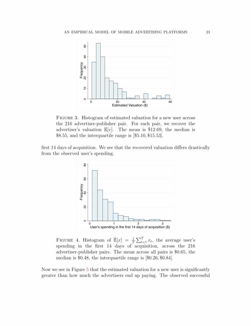
We plot the histogram of these valuation estimates in Figure 3.

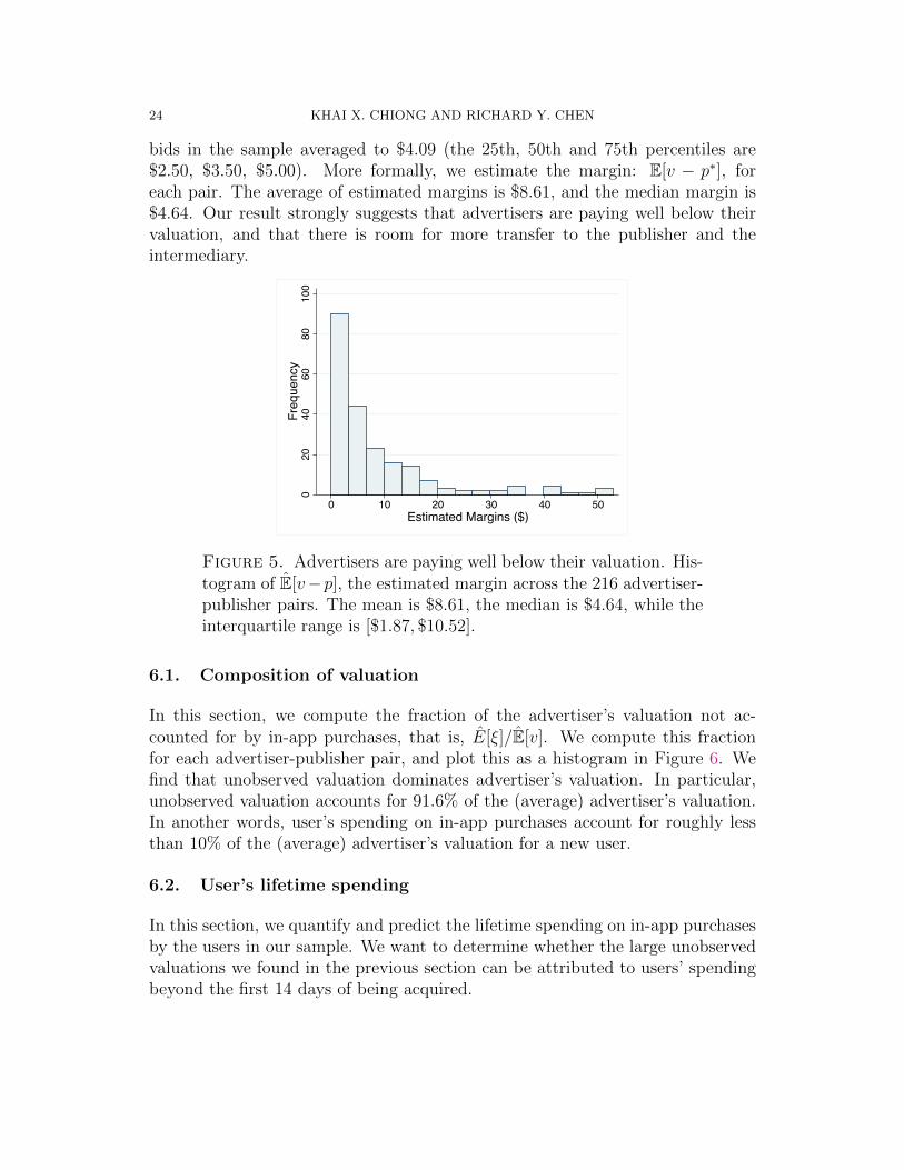
By comparison, we plot in Figure 4, the histogram of E[x] = 1T

∑Tt=1 xt, which is

the component of the overall valuation attributed to the user’s spending in the

E[v] =∑T

t=1 vt, of the advertiser for acquiring a user from the publisher is at least $0.10. See

the next section for construction of E[v].21For these 9 pairs, ∂Q(p)

∂p |p∗ in the moment condition (9) is almost zero.


010

2030

4050

Freq

uenc

y

0 20 40 60Estimated Valuation ($)

Figure 3. Histogram of estimated valuation for a new user acrossthe 216 advertiser-publisher pair. For each pair, we recover theadvertiser’s valuation E[v]. The mean is $12.69, the median is$8.55, and the interquartile range is [$5.10, $15.53].

first 14 days of acquisition. We see that the recovered valuation differs drasticallyfrom the observed user’s spending.

020

4060

80Fr

eque

ncy

0 1 2 3User's spending in the first 14 days of acquisition ($)

Figure 4. Histogram of E[x] = 1T

∑Tt=1 xt, the average user’s

spending in the first 14 days of acquisition, across the 216advertiser-publisher pairs. The mean across all pairs is $0.65, themedian is $0.48, the interquartile range is [$0.26, $0.84].

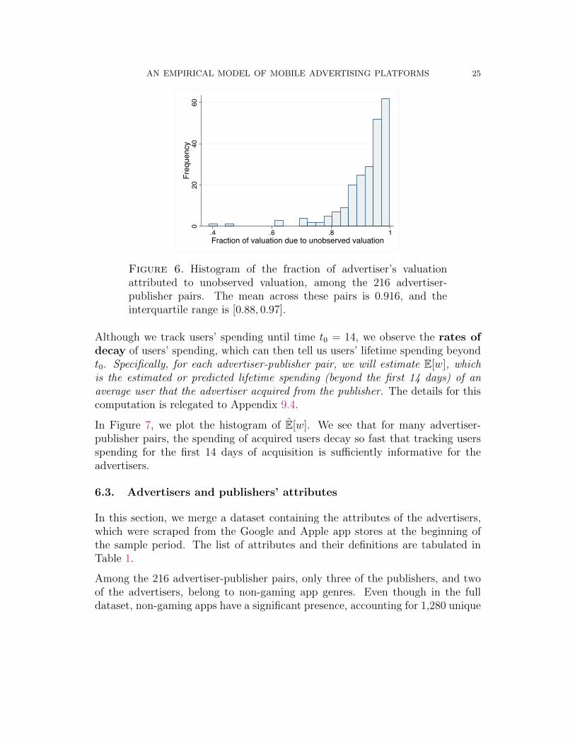
Now we see in Figure 5 that the estimated valuation for a new user is significantlygreater than how much the advertisers end up paying. The observed successful


bids in the sample averaged to $4.09 (the 25th, 50th and 75th percentiles are$2.50, $3.50, $5.00). More formally, we estimate the margin: E[v − p∗], foreach pair. The average of estimated margins is $8.61, and the median margin is$4.64. Our result strongly suggests that advertisers are paying well below theirvaluation, and that there is room for more transfer to the publisher and theintermediary.

020

4060

8010

0Fr

eque

ncy

0 10 20 30 40 50Estimated Margins ($)

Figure 5. Advertisers are paying well below their valuation. His-togram of E[v−p], the estimated margin across the 216 advertiser-publisher pairs. The mean is $8.61, the median is $4.64, while theinterquartile range is [$1.87, $10.52].

6.1. Composition of valuation

In this section, we compute the fraction of the advertiser’s valuation not ac-counted for by in-app purchases, that is, E[ξ]/E[v]. We compute this fractionfor each advertiser-publisher pair, and plot this as a histogram in Figure 6. Wefind that unobserved valuation dominates advertiser’s valuation. In particular,unobserved valuation accounts for 91.6% of the (average) advertiser’s valuation.In another words, user’s spending on in-app purchases account for roughly lessthan 10% of the (average) advertiser’s valuation for a new user.

6.2. User’s lifetime spending

In this section, we quantify and predict the lifetime spending on in-app purchasesby the users in our sample. We want to determine whether the large unobservedvaluations we found in the previous section can be attributed to users’ spendingbeyond the first 14 days of being acquired.


020

4060

Freq

uenc

y

.4 .6 .8 1Fraction of valuation due to unobserved valuation

Figure 6. Histogram of the fraction of advertiser’s valuationattributed to unobserved valuation, among the 216 advertiser-publisher pairs. The mean across these pairs is 0.916, and theinterquartile range is [0.88, 0.97].

Although we track users’ spending until time t0 = 14, we observe the rates ofdecay of users’ spending, which can then tell us users’ lifetime spending beyondt0. Specifically, for each advertiser-publisher pair, we will estimate E[w], whichis the estimated or predicted lifetime spending (beyond the first 14 days) of anaverage user that the advertiser acquired from the publisher. The details for thiscomputation is relegated to Appendix 9.4.

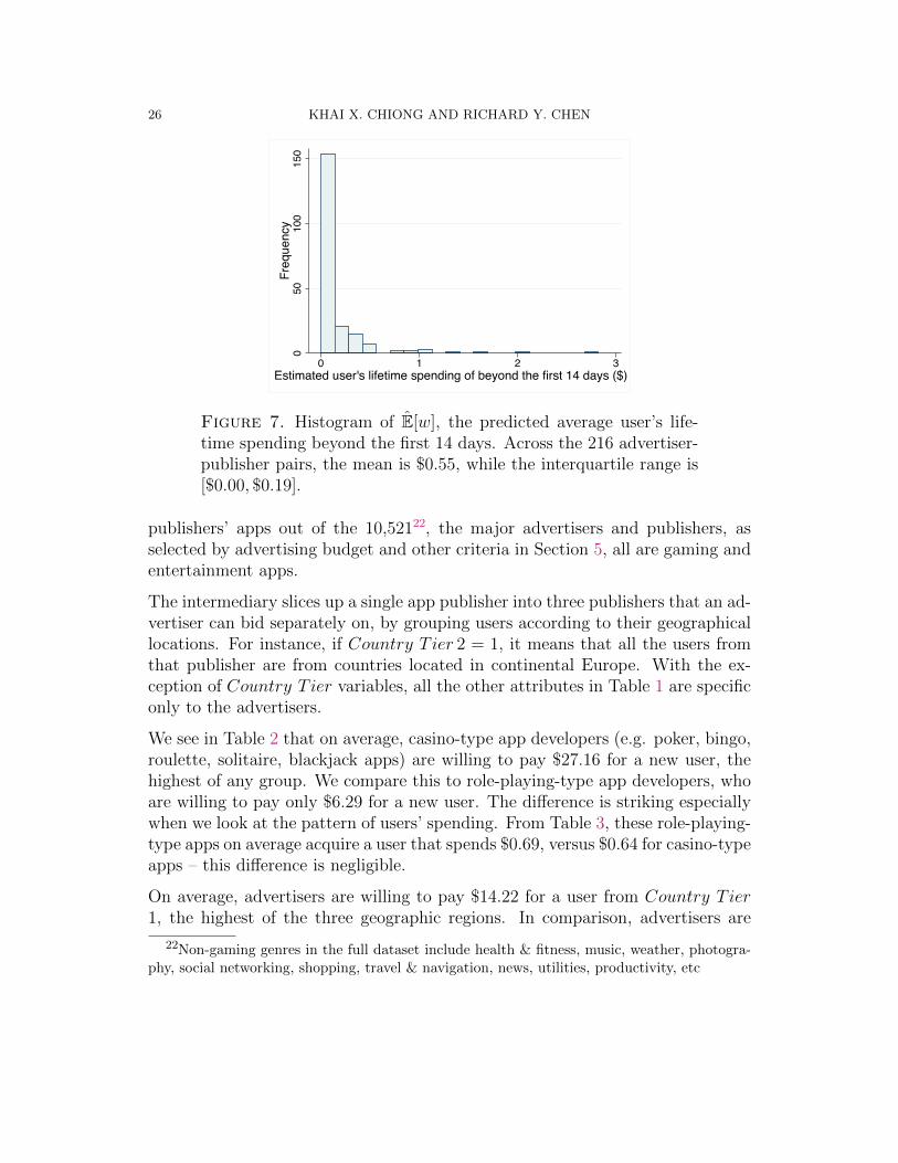
In Figure 7, we plot the histogram of E[w]. We see that for many advertiser-publisher pairs, the spending of acquired users decay so fast that tracking usersspending for the first 14 days of acquisition is sufficiently informative for theadvertisers.

6.3. Advertisers and publishers’ attributes

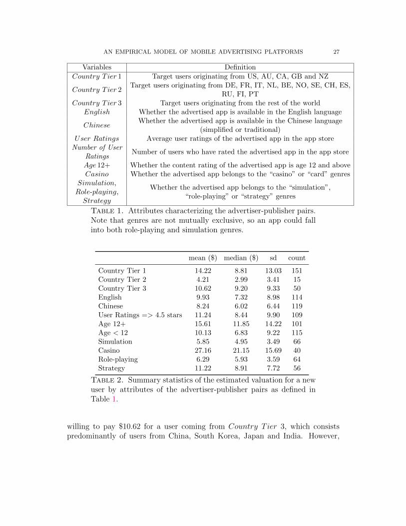
In this section, we merge a dataset containing the attributes of the advertisers,which were scraped from the Google and Apple app stores at the beginning ofthe sample period. The list of attributes and their definitions are tabulated inTable 1.

Among the 216 advertiser-publisher pairs, only three of the publishers, and twoof the advertisers, belong to non-gaming app genres. Even though in the fulldataset, non-gaming apps have a significant presence, accounting for 1,280 unique


050

100

150

Freq

uenc

y

0 1 2 3Estimated user's lifetime spending of beyond the first 14 days ($)

Figure 7. Histogram of E[w], the predicted average user’s life-time spending beyond the first 14 days. Across the 216 advertiser-publisher pairs, the mean is $0.55, while the interquartile range is[$0.00, $0.19].

publishers’ apps out of the 10,52122, the major advertisers and publishers, asselected by advertising budget and other criteria in Section 5, all are gaming andentertainment apps.

The intermediary slices up a single app publisher into three publishers that an ad-vertiser can bid separately on, by grouping users according to their geographicallocations. For instance, if Country T ier 2 = 1, it means that all the users fromthat publisher are from countries located in continental Europe. With the ex-ception of Country T ier variables, all the other attributes in Table 1 are specificonly to the advertisers.

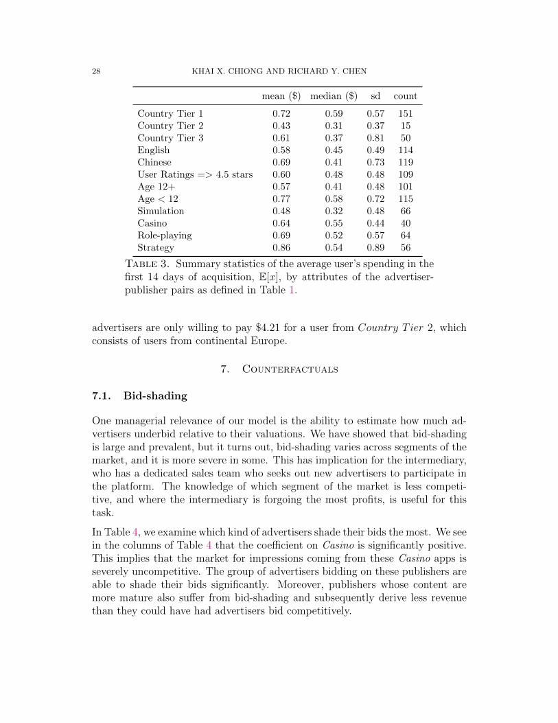
We see in Table 2 that on average, casino-type app developers (e.g. poker, bingo,roulette, solitaire, blackjack apps) are willing to pay $27.16 for a new user, thehighest of any group. We compare this to role-playing-type app developers, whoare willing to pay only $6.29 for a new user. The difference is striking especiallywhen we look at the pattern of users’ spending. From Table 3, these role-playing-type apps on average acquire a user that spends $0.69, versus $0.64 for casino-typeapps – this difference is negligible.

On average, advertisers are willing to pay $14.22 for a user from Country T ier1, the highest of the three geographic regions. In comparison, advertisers are

22Non-gaming genres in the full dataset include health & fitness, music, weather, photogra-phy, social networking, shopping, travel & navigation, news, utilities, productivity, etc


Variables Definition

Country T ier 1 Target users originating from US, AU, CA, GB and NZ

Country T ier 2Target users originating from DE, FR, IT, NL, BE, NO, SE, CH, ES,

RU, FI, PTCountry T ier 3 Target users originating from the rest of the world

English Whether the advertised app is available in the English language

ChineseWhether the advertised app is available in the Chinese language

(simplified or traditional)User Ratings Average user ratings of the advertised app in the app storeNumber of User

RatingsNumber of users who have rated the advertised app in the app store

Age 12+ Whether the content rating of the advertised app is age 12 and aboveCasino Whether the advertised app belongs to the “casino” or “card” genres

Simulation,Role-playing,Strategy

Whether the advertised app belongs to the “simulation”,“role-playing” or “strategy” genres

Table 1. Attributes characterizing the advertiser-publisher pairs.Note that genres are not mutually exclusive, so an app could fallinto both role-playing and simulation genres.

mean ($) median ($) sd count

Country Tier 1 14.22 8.81 13.03 151Country Tier 2 4.21 2.99 3.41 15Country Tier 3 10.62 9.20 9.33 50English 9.93 7.32 8.98 114Chinese 8.24 6.02 6.44 119User Ratings => 4.5 stars 11.24 8.44 9.90 109Age 12+ 15.61 11.85 14.22 101Age < 12 10.13 6.83 9.22 115Simulation 5.85 4.95 3.49 66Casino 27.16 21.15 15.69 40Role-playing 6.29 5.93 3.59 64Strategy 11.22 8.91 7.72 56

Table 2. Summary statistics of the estimated valuation for a newuser by attributes of the advertiser-publisher pairs as defined inTable 1.

willing to pay $10.62 for a user coming from Country T ier 3, which consistspredominantly of users from China, South Korea, Japan and India. However,


mean ($) median ($) sd count

Country Tier 1 0.72 0.59 0.57 151Country Tier 2 0.43 0.31 0.37 15Country Tier 3 0.61 0.37 0.81 50English 0.58 0.45 0.49 114Chinese 0.69 0.41 0.73 119User Ratings => 4.5 stars 0.60 0.48 0.48 109Age 12+ 0.57 0.41 0.48 101Age < 12 0.77 0.58 0.72 115Simulation 0.48 0.32 0.48 66Casino 0.64 0.55 0.44 40Role-playing 0.69 0.52 0.57 64Strategy 0.86 0.54 0.89 56

Table 3. Summary statistics of the average user’s spending in thefirst 14 days of acquisition, E[x], by attributes of the advertiser-publisher pairs as defined in Table 1.

advertisers are only willing to pay $4.21 for a user from Country T ier 2, whichconsists of users from continental Europe.

7. Counterfactuals

7.1. Bid-shading

One managerial relevance of our model is the ability to estimate how much ad-vertisers underbid relative to their valuations. We have showed that bid-shadingis large and prevalent, but it turns out, bid-shading varies across segments of themarket, and it is more severe in some. This has implication for the intermediary,who has a dedicated sales team who seeks out new advertisers to participate inthe platform. The knowledge of which segment of the market is less competi-tive, and where the intermediary is forgoing the most profits, is useful for thistask.

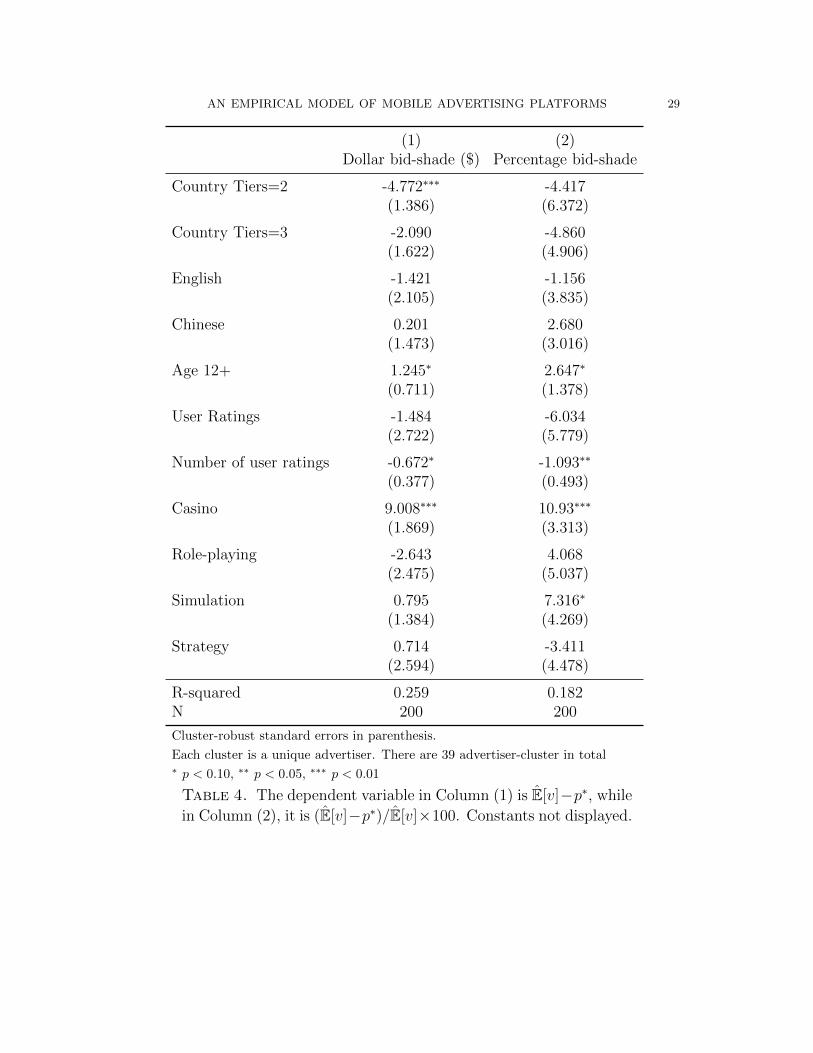
In Table 4, we examine which kind of advertisers shade their bids the most. We seein the columns of Table 4 that the coefficient on Casino is significantly positive.This implies that the market for impressions coming from these Casino apps isseverely uncompetitive. The group of advertisers bidding on these publishers areable to shade their bids significantly. Moreover, publishers whose content aremore mature also suffer from bid-shading and subsequently derive less revenuethan they could have had advertisers bid competitively.


(1) (2)Dollar bid-shade ($) Percentage bid-shade

Country Tiers=2 -4.772∗∗∗ -4.417(1.386) (6.372)

Country Tiers=3 -2.090 -4.860(1.622) (4.906)

English -1.421 -1.156(2.105) (3.835)

Chinese 0.201 2.680(1.473) (3.016)

Age 12+ 1.245∗ 2.647∗

(0.711) (1.378)

User Ratings -1.484 -6.034(2.722) (5.779)

Number of user ratings -0.672∗ -1.093∗∗

(0.377) (0.493)

Casino 9.008∗∗∗ 10.93∗∗∗

(1.869) (3.313)

Role-playing -2.643 4.068(2.475) (5.037)

Simulation 0.795 7.316∗

(1.384) (4.269)

Strategy 0.714 -3.411(2.594) (4.478)

R-squared 0.259 0.182N 200 200

Cluster-robust standard errors in parenthesis.

Each cluster is a unique advertiser. There are 39 advertiser-cluster in total∗ p < 0.10, ∗∗ p < 0.05, ∗∗∗ p < 0.01

Table 4. The dependent variable in Column (1) is E[v]−p∗, while

in Column (2), it is (E[v]−p∗)/E[v]×100. Constants not displayed.


7.2. Counterfactual bids: increasing competition

In this section, we use our estimated models to quantify the optimal responses(counterfactuals) of advertisers as a result of changes in the underlying modelparameters.

More specifically, we want to determine which publisher the intermediary shouldtarget the most, in terms of bringing in new advertisers to bid on that publisher.In practice, the intermediary has a sales team who pitches the platform to poten-tial advertisers. Moreover, once these advertisers joined the platform, the salesteam can then frame which publishers the new advertisers can bid on. Thereforeusing our tools here, we can guide this decision-making process of where to insertcompetition. The technical procedure for calculating the counterfactual bids isdeferred to Appendix 9.3.

Our counterfactual exercise is as follows: suppose each publisher were to gainan additional competing bidder, what are the advertisers’ profit-maximizing bidsgiven this new parameter? Using the procedure in Appendix 9.3, we compute theadvertisers’ counterfactual bids, and plot them as a histogram in Figure 8, whichshows the distribution of counterfactual bids for the 216 advertiser-publisherpairs. Further, we show in Figure 9 that advertisers’ bids would increase by about14.4% on average. As evident in Figure 9, increasing an additional bidder hasdifferent effects across publishers – it is more effective for some publishers.

7.3. Score boosting: artificial competition

One tweak to the mechanism that the intermediary can perform is to boost thequality scores of those bidders who would otherwise have a lower chance of win-ning. This is inefficient in the sense that the impression does not always go tothe bidder who promises the highest expected payment. On the surface then,the intermediary would suffer a loss. However, taking the endogeneity of bidsinto consideration, the other bidders with higher scores would now bid more ag-gressively due to this artificial increase in competition. Now if these advertisersincrease their bids sufficiently that it offsets fewer number of user acquisitions,then overall, the intermediary would receive a higher revenue.

Our counterfactual experiment proceeds as follows. There are two group of ad-vertisers, small and large. The large advertisers are the 40 advertisers we selected(among the 216 advertiser-publisher pairs) where their valuations are estimated.The second group are all the remaining advertisers.


020

4060

Freq

uenc

y

0 5 10 15 20Counterfactual bids ($)

Figure 8. If each publisher were to gain an additional bidder,then the resulting counterfactual bids has the distribution above.The mean is $4.91, and the interquartile range is [$3.26, $5.48].In comparison, the observed bids have a mean of $4.06, and aninterquartile range of [$3.00, $4.87].

020

4060

Freq

uenc

y

0 20 40 60 80 100Percentage increase in bids

Figure 9. On average, an advertiser’s bid would increase by about14.47%, with a median of 10.92%, and interquartile range of [6.33%,19.27%],

For each publisher among the 216 advertiser-publisher pairs, we look at all thesmall advertisers whose score-weighted bids lie in the bottom y-percentile of the


empirical score-weighted bids. We then boost the average score of these adver-tisers by a certain percentage. This results in a new empirical distribution ofscore-weighted bids Fc(·).

For each of the large advertiser, we calculate the counterfactual bid p in responseto this new empirical distribution of bids Fc(·). This is done by implementingthe iterative procedure described in Appendix 9.3. We then compute the expectedpayment to the intermediary: E[pQ(p)], where Q(p) = F (s · p)Nχs is the dailynumber of users that the advertiser would acquire in the counterfactuals. Here,F (·) is the counterfactual empirical distribution of score-weighted bids. Notethat χ does not depend on p so it can be estimated using the original non-counterfactual dataset as χ = Q(p∗)/(sF (s · p∗)N).

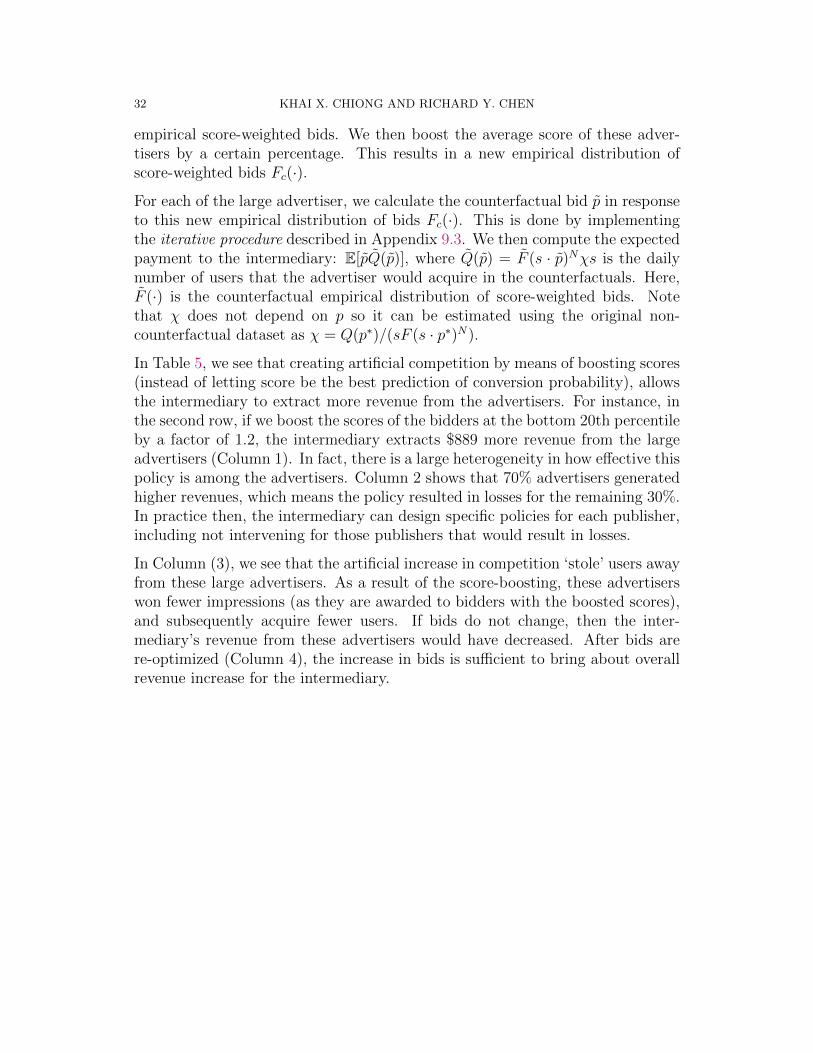
In Table 5, we see that creating artificial competition by means of boosting scores(instead of letting score be the best prediction of conversion probability), allowsthe intermediary to extract more revenue from the advertisers. For instance, inthe second row, if we boost the scores of the bidders at the bottom 20th percentileby a factor of 1.2, the intermediary extracts $889 more revenue from the largeadvertisers (Column 1). In fact, there is a large heterogeneity in how effective thispolicy is among the advertisers. Column 2 shows that 70% advertisers generatedhigher revenues, which means the policy resulted in losses for the remaining 30%.In practice then, the intermediary can design specific policies for each publisher,including not intervening for those publishers that would result in losses.

In Column (3), we see that the artificial increase in competition ‘stole’ users awayfrom these large advertisers. As a result of the score-boosting, these advertiserswon fewer impressions (as they are awarded to bidders with the boosted scores),and subsequently acquire fewer users. If bids do not change, then the inter-mediary’s revenue from these advertisers would have decreased. After bids arere-optimized (Column 4), the increase in bids is sufficient to bring about overallrevenue increase for the intermediary.


Experiments (1) (2) (3) (4)

Boost bottom 40th $914.77 64.4% -2.84 $0.76by 1.2

Boost bottom 20th $889.38 65.3% -2.53 $0.69by 1.2

Boost top 20th $81.6 59.0% -2.52 $0.68by 1.2

Boost middle 20th $373.2 60.8% -2.40 $0.71by 1.2

Table 5. Counterfactual experiments that are conducted for allpublishers. Column (1) reports the sum of revenue changes acrossall advertisers. Column (2): the percentage of advertisers whoserevenue changes are positive. Column (3): the median decrease inthe daily number of users acquired by those advertisers in whichrevenue changes are positive. Column (4): the median increase inbid among those advertisers with positive revenue changes.

8. Quantifying Resale Motives

8.1. Resale of users’ attention

We have seen the importance of advertisers’ unobserved valuations. In this sec-tion, we single out one possible explanation for what goes on in the advertiser’sunobserved valuation.

Due to the app-to-app advertising nature of our platform, an app developercan readily participate in both sides of the market, as both an advertiser and apublisher. This introduces resale motive which partly drives up the advertisers’valuations for a new user. More concretely, the advertiser perceives a user as adurable good, whereby a user generates a stream of diminishing monetary benefitsin terms of in-app purchases. Now the advertiser then has the option to resell auser by selling its impression and attention to other advertisers. By reselling theattention of the user, the user would potentially be drawn away to other apps(due to the scoring procedure used by the platform mechanism, the ads thatare shown to this user are often competing apps that are closely relevant to theuser).


Below we show more evidence that the resale motives of advertisers increase theirvaluations for new users.

8.2. Quantifying resale motives

For each pair of advertiser i and publisher j, we construct the variable πij captur-ing how much advertiser i expects to resell a user that is acquired from publisherj. Because this variable is not observed, we estimate πij using Equation (21)below.

πij = ηij × δij(21)

Where ηij is the number of impressions that advertiser i’s app can extract outfrom a user that was acquired from publisher j; and δij is the revenue per im-pression that advertiser i expects for a user that was acquired from publisherj.

Both ηij and δij are still not observed because only a subset of advertisers partic-ipate as publishers within our intermediary. Moreover an advertiser could resellusers’ attention and impression using other intermediaries, therefore we do notobserve the reselling activities of these advertisers. However, we do observe thecorresponding variables defined for publishers in our dataset. That is, we observethe number of impressions that a given publisher’s app extracts out from a userin a day; and the revenue per impression obtains by a publisher’s app in oursample.

The idea here is to assume that ηij and δij are functions of Xi and Yj, as in Equa-tions (22), (23) below, where Xi is the vector of attributes of the app where theimpression was generated (such as the app’s genre, language, users’ rating, matu-rity content rating, file size, cumulative number of installs); Yj is the attributesthat characterized user j’s impression. We take Yj to be a scalar attribute suchthat Yj = k if and only if user j belongs to Country Tier k for k = 1, 2, 3.23

23See Table 1 for definitions of Country Tiers. The intermediary allows advertisers to “slice”up a single publisher into multiple ones – by targeting different users from the same publisheraccording to users’ geographical locations.


ηij = η(Xi,Yj) + εij =3∑

k=1

1{Yj = k}Xiθk + εij(22)

δij = δ(Xi,Yj) + νij =3∑

k=1

1{Yj = k}Xiγk + νij(23)

The parameters θk and γk above can be estimated using the sample of publish-ers in our dataset. More precisely, we fit the data (ηij, δij,Xi, Yj)i∈P,j∈{1,2,3} toEquations (22) and (23), where P is the sample of publishers’ apps; ηij is the

observed number of impressions per type-j user for app i; δij is the observed adrevenue per impression received by app i, when the impression is generated by atype-j user.

In this estimation (fitting publishers’ impressions data to Equations 22 and 23),we use the full set of publishers available in our dataset, which totals to 15,562 ob-servations (i.e. 15,562 pairs of publisher/country-tier). This full set of publishersincludes thousands of publishers that we withheld from the structural estimation(see Section 5).

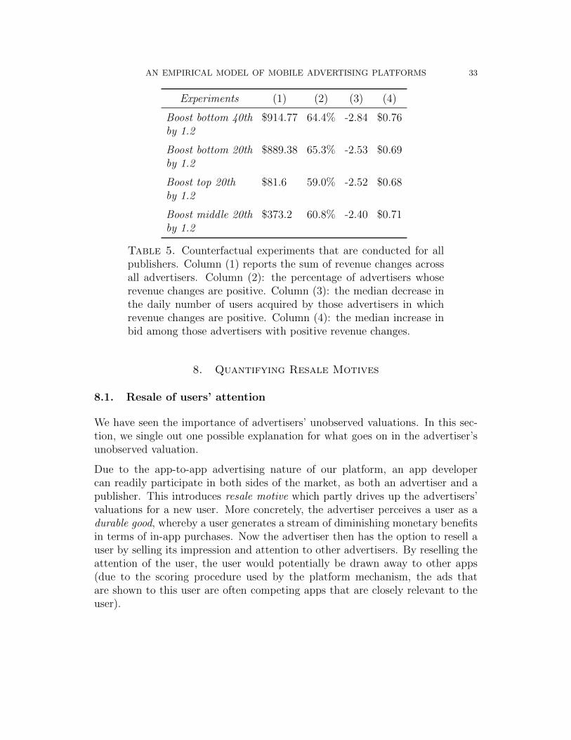
Note that the resale value constructed here is an underestimate of the actualresale value. There are two reasons. (1) We only observe impressions that aresold using our platform, which specialized in the niche of in-app video advertising.Publishers could enlist multiple platforms to sell impressions. (2) Our sampleperiod only covers 47 days from February 5, 2016 to March 22, 2016, we did notaccount for the lifetime number of impressions generated per user.

010

2030

40Fr

eque

ncy

0 .5 1 1.5Estimated Resale Value per User ($)

Figure 10. Estimated resale value of a user, πij, across 216advertiser-publisher pairs. The average resale value per user is$0.49, compare to $0.65 of in-app purchases generated per user.


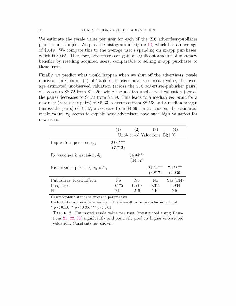
We estimate the resale value per user for each of the 216 advertiser-publisherpairs in our sample. We plot the histogram in Figure 10, which has an averageof $0.49. We compare this to the average user’s spending on in-app purchases,which is $0.65. Therefore, advertisers can gain a significant amount of monetarybenefits by reselling acquired users, comparable to selling in-app purchases tothese users.

Finally, we predict what would happen when we shut off the advertisers’ resalemotives. In Column (4) of Table 6, if users have zero resale value, the aver-age estimated unobserved valuation (across the 216 advertiser-publisher pairs)decreases to $8.72 from $12.26, while the median unobserved valuation (acrossthe pairs) decreases to $4.73 from $7.89. This leads to a median valuation for anew user (across the pairs) of $5.33, a decrease from $8.56; and a median margin(across the pairs) of $1.37, a decrease from $4.66. In conclusion, the estimatedresale value, πij seems to explain why advertisers have such high valuation fornew users.

(1) (2) (3) (4)

Unobserved Valuations, E[ξ] ($)

Impressions per user, ηij 22.05∗∗∗

(7.712)

Revenue per impression, δij 64.34∗∗∗

(14.82)

Resale value per user, ηij × δij 24.24∗∗∗ 7.123∗∗∗

(4.817) (2.230)

Publishers’ Fixed Effects No No No Yes (134)R-squared 0.175 0.279 0.311 0.934N 216 216 216 216



Table 6. Estimated resale value per user (constructed using Equa-tions 21, 22, 23) significantly and positively predicts higher unobservedvaluation. Constants not shown.


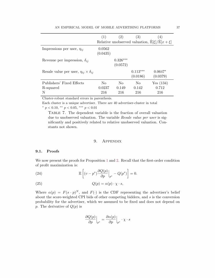
(1) (2) (3) (4)

Relative unobserved valuation, E[ξ]/E[x+ ξ]

Impressions per user, ηij 0.0562(0.0435)

Revenue per impression, δij 0.326∗∗∗

(0.0572)

Resale value per user, ηij × δij 0.113∗∗∗ 0.0647∗

(0.0186) (0.0379)

Publishers’ Fixed Effects No No No Yes (134)R-squared 0.0237 0.149 0.142 0.712N 216 216 216 216



Table 7. The dependent variable is the fraction of overall valuationdue to unobserved valuation. The variable Resale value per user is sig-nificantly and positively related to relative unobserved valuation. Con-stants not shown.

9. Appendix

9.1. Proofs

We now present the proofs for Proposition 1 and 2. Recall that the first-order conditionof profit maximization is:

(24) E[(v − p∗)∂Q(p)

∂p

∣∣∣p∗−Q(p∗)

]= 0.

(25) Q(p) = α(p) · χ · s,

Where α(p) = F (s · p)N , and F (·) is the CDF representing the advertiser’s beliefabout the score-weighted CPI bids of other competing bidders, and s is the conversionprobability for the advertiser, which we assumed to be fixed and does not depend onp. The derivative of Q(p) is

∂Q(p)

∂p

∣∣∣p∗

=∂α(p)

∂p

∣∣∣p∗· χ · s


Rewrite (24) using conditional expectation:

E[E[(v − p∗)|χ] · ∂Q(p)

∂p

∣∣∣p∗−Q(p∗)

]= 0.

Substituting the derivatives into the equation, we have

E[E[(v − p∗)|χ] · ∂α(p)

∂p

∣∣∣p∗· χ− α(p∗) · χ

]= 0,

Rewriting gets

E[χ · E[(v − p∗)|χ]] · ∂α(p)

∂p

∣∣∣p∗

= α(p∗)E[χ]

andα(p∗)∂α(p)∂p

∣∣∣p∗

=E[χ · E[(v − p∗)|χ]]

E[χ]

Finally we have,

α(p∗)/p∗

∂α(p)∂p

∣∣∣p∗

=1

p∗E[vχ]

E[χ]− 1

Where ρ = Cov(χ,v)E[χ]E[v] . Plugging in α(p) = F (s · p)N , we then have:

F (sp∗)

sNp∗f(sp∗)=

1

p∗E[vχ]

E[χ]− 1(26)

The RHS of Equation 26 is strictly decreasing in p∗, and we now show that the LHSof Equation 26 is strictly increasing in p∗ when F (·) is the CDF of a lognormaldistribution. Without loss of generality, we normalize N = 1.

In particular, when F (·) is the CDF of the lognormal distribution with parameter(µ, σ), that is, the random variable X drawn from the distribution F is such that logXis distributed N(µ, σ), then from Equation 26, we have:

√2πσe

(µ−log(sp))2

2σ2 Φ

(log(sp)− µ

σ

)=

E[v]

p(1 + ρ)− 1(27)

where Φ(·) is the CDF of the standard Gaussian. Denote the LHS of Equation 26 asL(p). Taking the partial derivative of L(p) with respect to p, we have that L(p) isstrictly increasing in p if


1 >√πey

2y erfc(y)(28)

Where y ≡ µ−log(ps)√2σ

, and erfc(y) is the complementary error function, i.e. erfc(y) =

1− 2√π

∫ y0 e−t2dt. Now denote l(y) ≡

√πey

2y erfc(y). We then show that l(y) is strictly

increasing in y, and that limy→∞ l(y) = 1. Therefore, the inequality in 28 above is truefor all y.

We will invoke two useful properties of the complementary error function.

erfc(y) ≥ 2√π

(e−y

2

y +√y2 + 2

)(29)

erfc(y)→ e−y2

y√π, as y →∞(30)

Equation 29 is a known lower bound of the complementary error function (Durrett,Probability: Theory and Examples, 3rd edition)24, while Equation 30 comes from theknown asymptotic expansion of erfc(y). From Equation 28 and 30, we can immediately

see that limy→∞√πey

2y erfc(y) = 1.

Now l′(y) =√πey

2 (2y2 + 1

)erfc(y)−2y, and plugging in the lower bound in Equation

29, we have l′(y) > 0 if2(2y2+1)√y2+2+y

− 2y > 0. This is true for all y.

Finally, we want to show that the LHS of Equation 27, i.e. converges to zero as p→ 0+.That is, limp→0+ L(p) = 0. Again this can be shown by invoking Equation 30:

L(p) =√

2πσe(µ−log(sp))2

2σ2 erfc

(µ− log(ps)√

2σ

)

→ e(µ−log(sp))2

2σ2

exp(−(µ−log(ps)√

2σ)2)

µ−log(ps)√2σ

√π

, as p→ 0+

=

√2πσ

µ− log(ps)

Therefore, limp→0+ L(p) = 0.

24Also, see http://mathworld.wolfram.com/Erfc.html


9.2. Summary statistics for the selected sample

We will present some summary statistics based on the sample of 222 advertiser-publisherpairs over the sample period of 47 days. There are 41 unique advertisers and 165 uniquepublishers among the 222 pairs. On average, (i) each advertiser spends a total of $5,719to acquire users from each publisher; (ii) each advertiser acquires a total of 1,399 usersfrom each publisher; (iii) each advertiser receives $796 in revenue generated by usersacquired from each publisher (tracking in-app purchases for 14 days after user acquisi-tion).

Overall in our sample, a single advertiser on average spends $31,260 throughout thesample period to acquire 7,577 number of users. On average, the advertiser receives$4,311 revenue from in-app purchases made by these new users (tracking revenue for thefirst 14 days). The winning CPI bids averaged over all incidences of user acquisitionsis $4.09, with a standard deviation of 2.72. The total number of users acquired in oursample is 310,657.

9.3. Procedure for computing counterfactual bids

Here, we show how the counterfactual bid is computed as we increase the number ofcompeting bidders N by one. We implement an iterative procedure to compute thecounterfactual bids as follows. For each publisher, there are two sets of advertisersbidding on it: large L, and small S. The large advertisers are the 40 advertisers we se-lected (among the 216 advertiser-publisher pairs) where their valuations are estimated.At the n-th iteration:

(1) Solve for the optimal bids p(n)i for i ∈ L, given the empirical distribution of

bids F(n)i (·) using Equation 31.

(2) Re-compute the empirical distribution of bids F(n+1)i (·) with p

(n)i replacing

p(n−1)i for i ∈ L.

Particularly for this counterfactual exercise, we always set N = N + 1. For a givenadvertiser-publisher pair and the corresponding (intermediate) counterfactual empirical

distribution F (n)(·), the counterfactual bid p(n) satisfies Equation 31 below.

E[χ((x+ ξ − p(n))∂α

(n)(p)

∂p

∣∣∣p(n)− α(n)(p(n))

)]= 0

=⇒(E[χx] + E[χξ]

)E[χ]

= p(n) +α(n)(p(n))∂α(n)(p)

∂p

∣∣∣p(n)

(31)

Since we observe the time-series of χ and x, we can then directly estimate E[χx] andE[χ]. Now using Equation 13, we can compute E[χξ] as follows.


E[χξ]

= E[E[χξ∣∣x, χ]]

= E[χE

[ξ∣∣x, χ]]

= E[χeβ0+β1x+β2q

]E[χξ]

=T∑t=1

(χte

β0+β1xt+β2qt)

The parameters (β0, β1, β2) are the ones we estimated between advertiser i and pub-lisher j from the two-steps GMM in Equation 19. The time-series qt is the daily numberof users acquired by the advertiser at the original non-counterfactual bid p∗. It remains

to specify α(n)(p) and ∂α(n)(p)∂p

∣∣∣p, which are given by:

α(n)(p) = F (n)(s · p)N

∂α(n)(p)

∂p

∣∣∣p

= NF (n)(s · p)N−1f (n)(s · p)s

9.4. Quantifying user’s lifetime in-app purchases

We begin with:

w =

∫ ∞t=t0

e−ρ(t−t0)w(t)dt

Where ρ is our discount rate and w(t) is the spending of the acquired user at timet. Therefore, the conditional expectation of E[w|x], where x is the acquired user’scumulative spending until t0, is given by:

E[w|x] =

∫ ∞t=t0

e−ρ(t−t0) E[w(t)|x]dt

Further, we assume that:

E[w(t)|x] = exp(a0 + a1t+ a2t

2 + a3x+ a4x2 + a5t · x

)(32)

The use of exponential form is appropriate here because spending takes positive values.We can estimate the unknown parameters (a0, . . . , a5) using Equation 32 since werecorded the spending w(t) of each acquired user at different point in time, as well as


the corresponding x, the acquired user’s cumulative spendings at time t0.25 Similar

to Chan et al. (2011), we set the continuous discount rate, ρ, to be 0.000611. Thiscorresponds to a 20% annual discount rate. We also examine whether the results aresensitive to using 15% discount rate.

Therefore, our predicted lifetime spending of an average user acquired from the pub-lisher is given by:

1

T

T∑t

(xt + E[w|xt])(33)

where

E[w|x] =

∫ ∞t=t0

e−ρ(t−t0)E[w(t)|x]dt(34)

and E[w(t)|v] is Equation (32) fitted to the data.

Acknowledgements

We thank Matt Shum, Sha Yang, Botao Yang, Ben Gillen, Marcelo Fernandez, KirillPogorelskiy, as well as seminar participants at UCLA, University of Florida and UTDallas.

References

Agarwal, N., Athey, S., and Yang, D. (2009). Skewed bidding in pay-per-action auctionsfor online advertising. The American Economic Review, 99(2):441–447.

Amaldoss, W., Desai, P. S., and Shin, W. (2015). Keyword search advertising andfirst-page bid estimates: A strategic analysis. Management Science, 61(3):507–519.

Andrews, M., Goehring, J., Hui, S., Pancras, J., and Thornswood, L. (2016). Mobilepromotions: A framework and research priorities. Journal of Interactive Marketing,34:15–24.

Andrews, M., Luo, X., Fang, Z., and Ghose, A. (2014). Mobile crowdsensing. MarketingScience forthcoming. Fox School of Business Research, pages 15–040.

Andrews, M., Luo, X., Fang, Z., and Ghose, A. (2015). Mobile ad effectiveness: Hyper-contextual targeting with crowdedness. Marketing Science.

25In estimating Equation 32, we use tracking data that spanned the first 30 days of useracquisition.


Asdemir, K., Kumar, N., and Jacob, V. S. (2012). Pricing models for online advertising:Cpm vs. cpc. Information Systems Research, 23(3-part-1):804–822.

Athey, S. and Nekipelov, D. (2010). A structural model of sponsored search advertisingauctions. In Sixth ad auctions workshop.

Bart, Y., Stephen, A. T., and Sarvary, M. (2014). Which products are best suited tomobile advertising? a field study of mobile display advertising effects on consumerattitudes and intentions. Journal of Marketing Research, 51(3):270–285.

Blake, T., Nosko, C., and Tadelis, S. (2015). Consumer heterogeneity and paid searcheffectiveness: A large-scale field experiment. Econometrica, 83(1):155–174.

Bruce, N., Murthi, B., and Rao, R. C. (2016). A dynamic model for digital advertis-ing: The effects of creative formats, message content and targeting on engagement.Message Content and Targeting on Engagement (April 10, 2016).

Chamberlain, G. (1987). Asymptotic efficiency in estimation with conditional momentrestrictions. Journal of Econometrics, 34(3):305–334.

Chan, T. Y., Kadiyali, V., and Park, Y.-H. (2007). Willingness to pay and competitionin online auctions. Journal of Marketing Research, 44(2):324–333.

Chan, T. Y., Wu, C., and Xie, Y. (2011). Measuring the lifetime value of customersacquired from google search advertising. Marketing Science, 30(5):837–850.

Chen, Y., Wang, Q., and Xie, J. (2011). Online social interactions: A natural experi-ment on word of mouth versus observational learning. Journal of marketing research,48(2):238–254.

Chen, Y. and Xie, J. (2008). Online consumer review: Word-of-mouth as a new elementof marketing communication mix. Management science, 54(3):477–491.

Fader, P. S. and Hardie, B. G. (2005). A note on deriving the pareto/nbd model andrelated expressions. http://www.brucehardie.com/notes/009/.

Fader, P. S., Hardie, B. G., and Lee, K. L. (2005). ‘counting your customers’ the easyway: An alternative to the pareto/nbd model. Marketing science, 24(2):275–284.

Fong, N. M., Fang, Z., and Luo, X. (2015). Geo-conquesting: Competitive locationaltargeting of mobile promotions. Journal of Marketing Research, 52(5):726–735.

Ghose, A. and Han, S. P. (2014). Estimating demand for mobile applications in thenew economy. Management Science, 60(6):1470–1488.

Ghose, A. and Yang, S. (2009). An empirical analysis of search engine advertising:Sponsored search in electronic markets. Management Science, 55(10):1605–1622.

Goldfarb, A. (2014). What is different about online advertising? Review of IndustrialOrganization, 44(2):115–129.


Goldfarb, A. and Tucker, C. (2011). Online display advertising: Targeting and obtru-siveness. Marketing Science, 30(3):389–404.

Grewal, D., Bart, Y., Spann, M., and Zubcsek, P. P. (2016). Mobile advertising: aframework and research agenda. Journal of Interactive Marketing, 34:3–14.

Gupta, S., Hanssens, D., Hardie, B., Kahn, W., Kumar, V., Lin, N., Ravishanker, N.,and Sriram, S. (2006). Modeling customer lifetime value. Journal of service research,9(2):139–155.

Hansen, L. P. (1982). Large sample properties of generalized method of momentsestimators. Econometrica: Journal of the Econometric Society, pages 1029–1054.

Hansen, L. P. and Singleton, K. J. (1982). Generalized instrumental variables esti-mation of nonlinear rational expectations models. Econometrica: Journal of theEconometric Society, pages 1269–1286.

Ho, T.-H., Li, S., Park, S.-E., and Shen, Z.-J. M. (2012). Customer influence value andpurchase acceleration in new product diffusion. Marketing Science, 31(2):236–256.

Hsieh, Y., Shum, M., and Yang, S. (2014). To score or not to score? structuralestimation of sponsored search auctions. Technical report, mimeo.

Hu, Y., Shin, J., and Tang, Z. (2015). Incentive problems in performance-based onlineadvertising pricing: Cost per click vs. cost per action. Management Science.

Iyer, G., Soberman, D., and Villas-Boas, J. M. (2005). The targeting of advertising.Marketing Science, 24(3):461–476.

Jeziorski, P. and Moorthy, S. (2016). Advertiser prominence effects in search advertis-ing. Working Paper.

Johnson, G. A. (2013). The impact of privacy policy on the auction market for onlinedisplay advertising.

Lambrecht, A. and Tucker, C. (2013). When does retargeting work? informationspecificity in online advertising. Journal of Marketing Research, 50(5):561–576.

Lee, C., Kumar, V., and Gupta, S. (2015). Designing freemium: Balancing growth andmonetization strategies. Available at SSRN.

Lewis, R. A. and Rao, J. M. (2015). The unfavorable economics of measuring thereturns to advertising*. The Quarterly Journal of Economics, page qjv023.

Liu, D. and Viswanathan, S. (2014). Information asymmetry and hybrid advertising.Journal of Marketing Research, 51(5):609–624.

Luo, X., Andrews, M., Fang, Z., and Phang, C. W. (2013). Mobile targeting. Manage-ment Science, 60(7):1738–1756.


Manchanda, P., Dube, J.-P., Goh, K. Y., and Chintagunta, P. K. (2006). The effect ofbanner advertising on internet purchasing. Journal of Marketing Research, 43(1):98–108.

Newey, W. K. (1985). Maximum likelihood specification testing and conditional mo-ment tests. Econometrica: Journal of the Econometric Society, pages 1047–1070.

Newey, W. K. (1993). 16 efficient estimation of models with conditional moment re-strictions. Handbook of statistics, 11:419–454.

Rutz, O. J. and Bucklin, R. E. (2011). From generic to branded: A model of spilloverin paid search advertising. Journal of Marketing Research, 48(1):87–102.

Sayedi, A., Jerath, K., and Srinivasan, K. (2014). Competitive poaching in sponsoredsearch advertising and its strategic impact on traditional advertising. MarketingScience, 33(4):586–608.

Schmittlein, D. C., Morrison, D. G., and Colombo, R. (1987). Counting your customers:Who-are they and what will they do next? Management science, 33(1):1–24.

Shankar, V. and Balasubramanian, S. (2009). Mobile marketing: a synthesis andprognosis. Journal of Interactive Marketing, 23(2):118–129.

Shin, W. (2015). Keyword search advertising and limited budgets. Marketing Science,34(6):882–896.

Sriram, S., Manchanda, P., Bravo, M. E., Chu, J., Ma, L., Song, M., Shriver, S.,and Subramanian, U. (2015). Platforms: a multiplicity of research opportunities.Marketing Letters, 26(2):141–152.

Trusov, M., Bucklin, R. E., and Pauwels, K. (2009). Effects of word-of-mouth versustraditional marketing: findings from an internet social networking site. Journal ofmarketing, 73(5):90–102.

Weintraub, G. Y., Benkard, C. L., and Van Roy, B. (2005). Oblivious equilibrium: Amean field approximation for large-scale dynamic games. In NIPS, pages 1489–1496.

Wu, C. (2015). Matching value and market design in online advertising networks: Anempirical analysis. Marketing Science, 34(6):906–921.

Yang, S. and Ghose, A. (2010). Analyzing the relationship between organic and spon-sored search advertising: Positive, negative, or zero interdependence? MarketingScience, 29(4):602–623.

Yao, S. and Mela, C. F. (2011). A dynamic model of sponsored search advertising.Marketing Science, 30(3):447–468.

Zhang, K. and Katona, Z. (2012). Contextual advertising. Marketing Science,31(6):980–994.


Zhu, Y. and Wilbur, K. C. (2011). Hybrid advertising auctions. Marketing Science,30(2):249–273.

Zubcsek, P. P., Katona, Z., and Sarvary, M. (2015). Social and location effects inmobile advertising. NA-Advances in Consumer Research Volume 43.

an empirical model of mobile advertising platforms

Documents