an empirical evaluation of alternative methods of ...an empirical evaluation of alternative methods...

An Empirical Evaluation of Alternative Methods of Estimation forConfirmatory Factor Analysis With Ordinal Data

David B. FloraArizona State University

Patrick J. CurranUniversity of North Carolina at Chapel Hill

Confirmatory factor analysis (CFA) is widely used for examining hypothesized relationsamong ordinal variables (e.g., Likert-type items). A theoretically appropriate method fits theCFA model to polychoric correlations using either weighted least squares (WLS) or robustWLS. Importantly, this approach assumes that a continuous, normal latent process determineseach observed variable. The extent to which violations of this assumption undermine CFAestimation is not well-known. In this article, the authors empirically study this issue using acomputer simulation study. The results suggest that estimation of polychoric correlations isrobust to modest violations of underlying normality. Further, WLS performed adequatelyonly at the largest sample size but led to substantial estimation difficulties with smallersamples. Finally, robust WLS performed well across all conditions.

Variables characterized by an ordinal level of measure-ment are common in many empirical investigations withinthe social and behavioral sciences. A typical situation in-volves the development or refinement of a psychometric testor survey in which a set of ordinally scaled items (e.g., 0 �strongly disagree, 1 � neither agree nor disagree, 2 �strongly agree) is used to assess one or more psychologicalconstructs. Although the individual items are designed tomeasure a theoretically continuous construct, the observedresponses are discrete realizations of a small number ofcategories. Statistical methods that assume continuous dis-tributions are often applied to observed measures that areordinally scaled. In circumstances such as these, there is thepotential for a critical mismatch between the assumptionsunderlying the statistical model and the empirical charac-teristics of the data to be analyzed. This mismatch in turnundermines confidence in the validity of the conclusions

that are drawn from empirical data with respect to a theo-retical model of interest (e.g., Shadish, Cook, & Campbell,2002).

This problem often arises in confirmatory factor analysis(CFA), a statistical modeling method commonly used inmany social science disciplines. CFA is a member of themore general family of structural equation models (SEMs)and provides a powerful method for testing a variety ofhypotheses about a set of measured variables. By far themost common method of estimation within CFA is maxi-mum likelihood (ML), a technique which assumes that theobserved variables are continuous and normally distributed(e.g., Bollen, 1989, pp. 131–134). These assumptions arenot met when the observed data are discrete (as occurs whenusing ordinal scales), thus significant problems can resultwhen fitting CFA models for ordinal scales using ML esti-mation (e.g., B. Muthen & Kaplan, 1985). Although severalalternative methods of estimation have been available forsome time, these have only recently become more accessi-ble to applied researchers through the continued develop-ment of SEM software. Despite this increased availability,key unanswered questions remain about the accuracy, va-lidity, and empirically informed guidelines for the optimaluse of these methods, particularly with respect to conditionscommonly encountered in behavioral research. The goal ofour article was to systematically and empirically addressseveral of these important questions.

Structural Equation Modeling (SEM)

SEM is a powerful and flexible analytic method that playsa critically important role in many empirical applications insocial science research. Because the general linear model is

David B. Flora, Department of Psychology, Arizona State Uni-versity; Patrick J. Curran, Department of Psychology, Universityof North Carolina at Chapel Hill.

Additional materials are on the web at http://dx.doi.org/10.1037/1082-989X.9.4.466.supp.

Portions of this research were presented at the annual meeting ofthe Psychometric Society in Chapel Hill, North Carolina, June2002. We are grateful for valuable input from Dan Bauer, KenBollen, Andrea Hussong, Abigail Panter, and Jack Vevea. Thiswork was supported in part by a dissertation award presented bythe Society of Multivariate Experimental Psychology to David B.Flora and Grant DA13148 awarded to Patrick J. Curran.

Correspondence should be addressed to Patrick J. Curran, De-partment of Psychology, University of North Carolina, ChapelHill, NC 27599-3270. E-mail: [email protected]

Psychological Methods2004, Vol. 9, No. 4, 466–491

Copyright 2004 by the American Psychological Association1082-989X/04/$12.00 DOI: 10.1037/1082-989X.9.4.466

466

embedded within SEM, this modeling framework can beused in a wide variety of applications. The general goal ofSEM is to test the hypothesis that the observed covariancematrix for a set of measured variables is equal to thecovariance matrix implied by an hypothesized model. Thisrelationship can be formally stated as

� � ��, (1)

where � represents the population covariance matrix of aset of observed variables and �(�) represents the populationcovariance matrix implied by �, a vector of model param-eters. The vector � thus defines the form of a particular SEMthrough the specification of means and intercepts, variancesand covariances, regression parameters, and factor loadings.

A particular parameterization of � leads to the well-known CFA model (Joreskog, 1969). In CFA, the covari-ance matrix implied by � is a function of �, a matrix ofvariances and covariances among latent factors; �, a matrixof factor loadings; and ��, a matrix of measurement errors(i.e., uniqueness). The model-implied covariance structureis

�� . (2)

Usual assumptions for CFA are that the model is properlyspecified (i.e., the model hypothesized in Equation 2 corre-sponds directly to the model that exists in the population),that �� is independent of the vector � of latent factors, andthat the measurement errors themselves are uncorrelated(i.e., �� is a diagonal matrix), although this latter conditionis to some degree testable.

ML is the most commonly applied method for estimatingthe model parameters in �. In addition to the usual CFAassumptions named above, ML assumes that the samplecovariance matrix is computed on the basis of continuous,normally distributed variables.1 Given adequate samplesize, proper model specification, and multivariately nor-mally distributed data (or more specifically, no multivariatekurtosis; Browne, 1984), ML provides consistent, efficient,and unbiased parameter estimates and asymptotic standarderrors as well as an omnibus test of model fit (Bollen, 1989;Browne, 1984).

However, in many applications in the behavioral sci-ences, the observed variables are not continuously distrib-uted.2 Instead, variables are often observed on a dichoto-mous or ordinal scale of measurement. It is well-knownfrom both statistical theory and prior simulation studies thatML based on the sample product–moment correlation orcovariance matrix among ordinal observed variables doesnot perform well, especially when the number of observedcategories is small (e.g., five or fewer). In particular, thechi-square model fit statistic is inflated (Babakus, Ferguson,& Joreskog, 1987; Green, Akey, Fleming, Hershberger, &Marquis, 1997; Hutchinson & Olmos, 1998; B. Muthen &Kaplan, 1992), parameters are underestimated (Babakus et

al., 1987; B. Muthen & Kaplan, 1992), and standard errorestimates tend to be downwardly biased (B. Muthen &Kaplan, 1985, 1992). An alternative approach to estimatingCFA models for ordinal observed data involves the estima-tion and analysis of polychoric and polyserial correlations.

Polychoric Correlations

There is a long history of theory and research with poly-choric and polyserial correlations dating back to Pearson(1901). The polychoric correlation estimates the linear re-lationship between two unobserved continuous variablesgiven only observed ordinal data, whereas the polyserialcorrelation measures the linear relationship between twocontinuous variables when only one of the observed distri-butions is ordinal and the other is continuous. Thus, calcu-lation of a polychoric correlation is based on the premisethat the observed discrete values are due to an unobservedunderlying continuous distribution. We adopt the terminol-ogy of B. Muthen (1983, 1984) to refer to an unobservedunivariate continuous distribution that generates an ob-served ordinal distribution as a latent response distribution.

The relationship between a latent response distribution,y*, and an observed ordinal distribution, y, is formalized as

y � c, if �c � y* � �c�1, (3)

with thresholds � as parameters defining the categories c �0, 1, 2, . . . , C � 1, where �0 � �� and �C � �. Hence, theobserved ordinal value for y changes when a threshold � isexceeded on the latent response variable y*. The primaryreason that ML based on sample product–moment relation-ships does not perform well with ordinal observed data isthat the covariance structure hypothesis (see Equation 1)holds for the latent response variables but does not generallyhold for the observed ordinal variables (Bollen, 1989, p.434).

Polychoric correlations are typically calculated using thetwo-stage procedure described by Olsson (1979). In the firststage, the proportions of observations in each category of aunivariate ordinal variable are used to estimate the thresholdparameters for each univariate latent response variable sep-arately. Formally, for an observed ordinal variable y1, withthresholds denoted by ai, i � 0, . . . , s, and y2, with thresh-olds denoted by bj, j � 0, . . . , r, the first step is to estimate

ai � �1�1�Pi�� (4)

1 This assumption specifically applies to endogenous variables,or residuals (see Bollen, 1989, pp. 126–127). Given our focus onthe CFA model, all observed variables are endogenous here.

2 Strictly speaking, all observed measurements are discrete, buthere we are talking about coarse categorization of a theoreticallycontinuous distribution resulting in a small number of discretelevels.

467ORDINAL CFA

and

bj � �1�1�P �j�, (5)

where Pij is the observed proportion in cell (i, j), Pi� and P�j

are observed cumulative marginal proportions of the con-tingency table of y1 and y2, and �1

�1 represents the inverseof the univariate standard normal cumulative distributionfunction. In the second stage, these estimated thresholdparameters are used in combination with the observed bi-variate contingency table to estimate, via maximum likeli-hood, the correlation that would have been obtained had thetwo latent response variables been directly observed. Thelog-likelihood of the bivariate sample is

� � ln K � �i�1

s �j�1

r

ni,jln �i,j, (6)

where K is a constant, ni,j denotes the frequency of obser-vations in cell (i, j), and �i,j denotes the probability that agiven observation falls into cell (i, j) (Olsson, 1979).

Critically important in the calculation of a polychoriccorrelation is the assumption that the pair of latent responsevariables has a bivariate normal distribution. This assump-tion becomes evident in the reference to the univariatestandard normal distribution in the calculation of the thresh-olds (see Equations 4 and 5). Under the assumption ofbivariate normality for y*1 and y*2, Olsson (1979) gave theprobability �i,j (see Equation 6) that an observation fallsinto a given cell of the contingency table for y1 and y2 as

�i,j � �2�ai, bj� � �2�ai�1, bj� � �2�ai, bj�1�

� �2�ai�1, bj�1�, (7)

where �2 is the bivariate normal cumulative density func-tion with correlation �. The ML estimate of � yields thepolychoric correlation between the observed ordinal vari-ables y1 and y2. Olsson reported limited simulation resultsshowing that this two-stage method for calculating a poly-choric correlation between two ordinal variables gives anunbiased estimate of the correlation between a pair of bi-variate normal latent response variables.

Although the assumption of bivariate normality for latentresponse variables has been criticized as unrealistic in prac-tice (e.g., Lord & Novick, 1968; Yule, 1912), other re-searchers have advocated the practical convenience of thisassumption (e.g., B. Muthen & Hofacker, 1988; Pearson &Heron, 1913). Specifically, regardless of whether a pair ofobserved ordinal variables represents the realization of acategorized bivariate normal distribution or some other bi-variate continuous distribution, if the continuous distribu-tions are correlated, one would expect to see evidence forthis correlation in the observed contingency table for thetwo ordinal variables. That is, for a positive correlation,inspection of the relative frequencies in the individual cells

of the contingency table for the two ordinal variables wouldbe expected to reflect that lower values on one ordinalvariable would be associated with lower values on the otherordinal variable, whereas higher values on one variablewould be associated with higher values on the other. Giventhat the contingency table supplies the only observed datafor estimation of the correlation between the latent contin-uous variables, it is necessary to specify some (albeit un-known) distribution for the underlying continuous variablesto allow estimation of their correlation. Because of itswell-known mathematical properties, the assumption of abivariate normal distribution considerably facilitates estima-tion of the correlation, as shown in Equations 4–7. Al-though two correlated nonnormal y* variables would beexpected to generate a contingency table with similar pat-terns to that observed for two normal y* variables with thesame correlation, the extent to which calculation of thepolychoric correlation is robust to this nonnormality re-mains a matter of empirical investigation. Our goal in thisarticle was to pursue such an empirical examination.

To our knowledge, Quiroga (1992) represents the onlysimulation study that has empirically evaluated the accuracyof polychoric correlations under violations of the latentnormality assumption. Quiroga manipulated the skewnessand kurtosis of two continuous variables (i.e., y* variables)to examine the effects of nonnormality on polychoric cor-relation estimates between two variables, each with fourobserved ordinal categories. The polychoric correlation val-ues consistently overestimated the true correlation betweenthe nonnormal latent response variables. However, the ex-tent of the overestimation was small, with bias typically lessthan 2% of the true correlation. Although the findings ofQuiroga suggest that polychoric correlations are typicallyrobust to violation of the underlying y* normality assump-tion, to our knowledge no prior studies have examined theeffect of violating this assumption on fitting CFAs to poly-choric correlations. That is, demonstrating lack of bias inthe estimation of polychoric correlations is necessary butnot sufficient for inferring the robustness of CFAs fitted tothese correlations more generally. This is particularly sa-lient when considering alternative methods for fitting thesemodels in practice. Two important methods of interest to usin this article are fully weighted least squares (WLS) androbust WLS.

WLS Estimation

Both analytical and empirical work have demonstratedthat simply substituting a matrix of polychoric correlationsfor the sample product–moment covariance matrix in theusual ML estimation function for SEM is inappropriate.Although this approach will generally yield consistent pa-rameter estimates, it is known to produce incorrect teststatistics and standard errors (Babakus et al., 1987; Dolan,1994; Rigdon & Ferguson, 1991). Over the past several

468 FLORA AND CURRAN

decades, a WLS approach has been developed for estimat-ing a weight matrix based on the asymptotic variances andcovariances of polychoric correlations that can be used inconjunction with a matrix of polychoric correlations in theestimation of SEM models (e.g., Browne, 1982, 1984;Joreskog, 1994; B. Muthen, 1984; B. O. Muthen & Satorra,1995).

WLS applies the fitting function

FWLS � �s � ��W�1�s � ��, (8)

where s is a vector of sample statistics (i.e., polychoric corre-lations), �(�) is the model-implied vector of population ele-ments in �(�), and W is a positive-definite weight matrix.Browne (1982, 1984) showed that if a consistent estimator ofthe asymptotic covariance matrix of s is chosen for W, thenFWLS leads to asymptotically efficient parameter estimates andcorrect standard errors as well as a chi-square-distributedmodel test statistic. Furthermore, Browne (1982, 1984) pre-sented formulae for estimating the correct asymptotic covari-ance matrix in the context of continuously distributed observeddata using observed fourth-order moments. Because these for-mulae hold without specifying a particular distribution for theobserved variables, FWLS is often called the asymptoticallydistribution free (ADF) estimator when used with a correctasymptotic covariance matrix.

Browne (1982, 1984) primarily focused on WLS as ap-plied to continuous but nonnormal distributions, whereas B.Muthen (1983, 1984) presented a “continuous/categoricalvariable methodology” (CVM) for estimating SEMs thatallows any combination of dichotomous, ordered categori-cal, or continuous observed variables. With CVM, bivariaterelationships among ordinal observed variables are esti-mated with polychoric correlations, and the SEM is fit usingWLS estimation. The key contribution of CVM is that itessentially generalizes Browne’s work with FWLS beyondthe case of continuous observed data, as Muthen describedthe estimation of the correct asymptotic covariance matrixamong polychoric correlation estimates (B. Muthen, 1984;B. O. Muthen & Satorra, 1995). Thus, unlike normal-theoryestimation, CVM provides asymptotically unbiased, consis-tent, and efficient parameter estimates as well as a correctchi-square test of fit with dichotomous or ordinal observedvariables. Parallel but independent research by Joreskog(Joreskog, 1994; Joreskog & Sorbom, 1988) similarly gen-eralized Browne’s work to the estimation of the correct as-ymptotic covariance matrix among polychoric correlations.3

Despite its asymptotic elegance, there are two potentiallimitations of full WLS estimation in research applicationsof CFA with ordinal data. First, although limited priorsimulation evidence suggests that the computation of poly-choric correlations is generally robust to violations of thelatent normality assumption (Quiroga, 1992), to our knowl-edge the ramifications of these violations for the estimationof asymptotic covariances among polychoric correlations

have yet to be considered. Thus, although polychoric cor-relations may be generally unbiased, CFA model test sta-tistics and standard errors might be adversely affected be-cause of biases in the asymptotic covariance matrixintroduced by nonnormality among latent response vari-ables. Second, a frequent criticism against full WLS esti-mation is that the dimensions of the optimal weight matrixW are typically exceedingly large and increase rapidly as afunction of the number of indicators in a model. By virtueof its size in the context of a large model (i.e., a model withmany observed variables), W is often nonpositive definiteand cannot be inverted when applying the WLS fittingfunction (e.g., Bentler, 1995; West, Finch, & Curran, 1995).Furthermore, calculation of these asymptotic values re-quires a large sample size to produce stable estimates.Specifically, Joreskog and Sorbom (1996) suggested that aminimum sample size of (k � 1)(k � 2)/2, where k is thenumber of indicators in a model, should be available forestimation of W. As the elements of W have substantialsampling variability when based on small sample sizes, thisinstability has an accumulating effect as the number ofindicators in the model increases (Browne, 1984).

Thus, it is well-known that significant problems arisewhen using full WLS estimation in conditions commonlyencountered in social science research. Simulation studieshave shown that chi-square test statistics are consistentlyinflated when ADF estimation is applied to sample product–moment covariance or correlation matrices of continuousobserved data (e.g., Chou & Bentler, 1995; Curran, West, &Finch, 1996; Hu, Bentler, & Kano, 1992). Similarly, simu-lation studies applying WLS estimation to the analysis ofpolychoric correlation matrices have also reported inflatedchi-square test statistics (Dolan, 1994; Hutchinson & Ol-mos, 1998; Potthast, 1993) and negatively biased standarderror estimates (Potthast, 1993). In particular, both Dolanand Potthast reported that these problems worsen as a func-tion of increasing model size (i.e., number of indicators) anddecreasing sample size. Thus, full WLS is often of limitedusefulness in many applied research settings.

Robust WLS

To address the problems encountered when using fullWLS with small to moderate sample sizes, B. Muthen, duToit, and Spisic (1997; see also L. K. Muthen & Muthen,1998, pp. 357–358) presented a robust WLS approach that

3 Although the methods of B. Muthen and Joreskog for estimat-ing the asymptotic covariance matrix are highly similar, they differin their treatment of the threshold parameters categorizing latentresponse distributions into observed ordinal distributions. Thesimulation study by Dolan (1994) suggested that the Joreskogapproach to estimating the asymptotic covariance matrix elicitsvirtually identical results as the Muthen approach with respect tothe estimation of CFA models.

469ORDINAL CFA

is based on the work of Satorra and colleagues (Chou,Bentler, & Satorra, 1991; Satorra, 1992; Satorra & Bentler,1990).4 With this method, parameter estimates are obtainedby substituting a diagonal matrix, V, for W in Equation 8,the elements of which are the asymptotic variances of thethresholds and polychoric correlation estimates (i.e., thediagonal elements of the original weight matrix). Once avector of parameter estimates is obtained, a robust asymp-totic covariance matrix is used to obtain parameter standarderrors. Calculation of this matrix involves the full weightmatrix W; however, it need not be inverted. Next, Muthenet al. described a robust goodness-of-fit test via calculationof a mean- and variance-adjusted chi-square test statistic.Calculation of this test statistic also involves the full weightmatrix W but similarly avoids inversion. An interestingaspect of this robust WLS method is that the value for themodel degrees of freedom is estimated from the empiricaldata, in a manner inspired by Satterthwaite (1941; cited inSatorra, 1992), rather than being determined directly fromthe specification of the model. The robust goodness-of-fittest presented by Muthen et al. essentially involves the usualchi-square test statistic multiplied by an adjustment akin tothe Satorra and Bentler (1986, 1988) robust chi-square teststatistic, with model degrees of freedom estimated from thedata.5 Detailed formulae describing estimation of standarderrors and model fit statistics with robust WLS were givenby B. Muthen et al. as well as by L. K. Muthen and Muthen(1998, pp. 357–358).

The Current Study

Our motivating goal was to provide an empirical evalu-ation of a set of specific hypotheses derived from the sta-tistical theory underlying the calculation of polychoric cor-relations and their use in estimating CFAs in appliedresearch. A small number of simulation studies, most nota-bly by Potthast (1993; see also Babakus et al., 1987; Dolan,1994; Hutchinson & Olmos, 1998), have previously evalu-ated the use of polychoric correlations with full WLS esti-mation for CFA. In each of these studies, researchers gen-erated y* variables from continuous, multivariate normaldata with known factor structures. Different sets of thresh-old values were then applied to these normal y* variables tocreate ordinal y variables with varying observed distribu-tions. These studies generally found that as the skewness orpositive kurtosis of the observed (ordinal) variables de-parted from zero, the estimation of the known factor struc-ture among the unobserved normal y* variables deteriorateddespite that the statistical theory underlying CFA with poly-choric correlations makes no explicit assumption about theskewness and kurtosis of the observed ordinal variables.This finding likely occurred in part because highly kurtoticordinal distributions produce contingency tables with lowexpected cell frequencies, which Olsson (1979) speculatedwould lead to poor polychoric correlation estimates and

which Brown and Bendetti (1977) showed would lead tobiased tetrachoric correlations.6

In the present study, rather than manipulating the thresh-old values along normal y* distributions to generate y vari-ables of varying observed skewness and kurtosis, we insteadmanipulated the unobserved skewness and kurtosis of the y*variables. In this way, we directly evaluated robustness ofCFA with polychoric correlations under violation of theexplicit, theoretical assumption that y* variables underlyingpolychoric correlations be normally distributed. Further-more, if there is little practical consequence to violation ofthe latent normality assumption, we will have partiallydemonstrated that this assumption merely provides a math-ematical convenience facilitating the calculation of correla-tions among latent response variables, as implied by Pear-son and Heron (1913) and B. Muthen and Hofacker (1988).7

Thus, our study focused on the systematic variation of theunobserved distribution of y* rather than on the observeddistribution of y. This is an important distinction given thatmanipulation of the latter has been the sole focus of priorresearch (e.g., Potthast, 1993).

Statistical theory and prior empirical findings have high-lighted three issues of critical importance when consideringthe estimation of CFA models (and SEMs in general) usingpolychoric correlations. First, although limited evidencesuggests that polychoric correlations are robust to violationsof bivariate normality for continuous latent response vari-ables eliciting observed ordinal variables, we are aware ofno prior research examining whether this robustness extendsto the estimation of CFA model parameters, test statistics,and standard errors using WLS estimation with a correctasymptotic covariance matrix. Second, we are aware of noprior research examining the stability and accuracy of ro-bust WLS under either bivariate normality or bivariatenonnormality for latent response variables. This is a prom-ising method for use in social science research, and the finitesample performance of robust WLS is an issue of key

4 Joreskog and Sorbom (1996) described a similar approach,termed diagonally weighted least squares.

5 A drawback of this robust WLS method is that the robustchi-square values cannot be used to compare nested models be-cause the degrees of freedom may vary within a given modelspecification.

6 The tetrachoric correlation is a special case of the polychoriccorrelation where both observed variables are dichotomous.

7 It is possible to create any ordinal distribution from a normaldistribution given the correct set of threshold values. Likewise,given an observed ordinal distribution in a practical setting (i.e.,not an artificially simulated distribution), it is impossible to knowwhether it was generated from a normal or nonnormal continuousvariable. However, applied researchers may be highly skeptical ofwhether it is realistic to assume that the latent response variable isin fact normal (e.g., it may represent propensity toward an abnor-mal behavior, such as illegal drug use).


interest. Finally, we are not aware of any existing systematicstudy that explores these questions with respect to thespecific number of discrete levels observed in the ordinalscale; this has significant implications in the design of itemresponse scales in anticipation of using these techniques inpractice. We explore all three of these issues in detail in thisarticle.

We drew on statistical theory and prior empirical researchto generate several hypotheses that we empirically exam-ined using a comprehensive computer simulation study.First, consistent with Quiroga (1992), we predicted that theestimates of polychoric correlations would be relativelyunbiased as a function of minor to modest violations ofnormality of the latent response distributions. Next, we hadseveral hypotheses pertaining to full WLS estimation ofCFA models using polychoric correlations. Consistent withDolan (1994) and Potthast (1993), we predicted that fullWLS would lead to inflated test statistics and underesti-mated parameter standard errors and that these biases wouldworsen substantially as a function of increasing model size(i.e., number of indicators) and decreasing sample size.Although we focused on the chi-square test statistics as aprimary outcome, this was essentially an examination of thediscrepancy function upon which all commonly used fitindices for SEM are based. Thus, conditions that contributeto inflated chi-square values were also expected to contrib-ute to bias in other fit indices, causing them also to suggestpoorer fit.

A polychoric correlation matrix is a consistent estimatorof the population correlation matrix for continuous latentresponse variables. Thus, like Rigdon and Ferguson (1991)and Potthast (1993), we expected to find unbiased parameterestimates independently of sample size and model complex-ity. However, because nonnormality in latent response dis-tributions may introduce small positive biases in polychoriccorrelations (Quiroga, 1992), we predicted that nonnormal-ity in latent response distributions would create modestlypositively biased parameter estimates. Further, because cal-culation of the asymptotic covariance matrix among poly-choric correlations takes into account fourth-moment infor-mation based on the distribution-free technique of Browne(1984), we did not predict that underlying nonnormalitywould have a substantial effect on full WLS chi-square teststatistics or standard errors at larger sample sizes for lesscomplex models.

Finally, like full WLS estimation, we expected that robustWLS would result in unbiased parameter estimates withnormal latent response distributions and modestly overesti-mated parameters with nonnormal latent response distribu-tions. Drawing from the results of Curran et al. (1996)relating to the Satorra–Bentler corrections applied to non-normal but continuous measures, we predicted that robustWLS would generally produce unbiased parameter standard

errors and test statistics across a wider range of sample sizesand model complexity than would full WLS. However, it isnot known to what degree robust WLS would provideaccurate estimates at the smallest sample sizes for the mostcomplex models. Taken together, we believe that our resultsmake unique contributions both to the understanding of thefinite sampling properties of these asymptotic estimatorsand to the provision of recommendations for applied re-searchers using these methods in practice.

Method

We used Monte Carlo computer simulation methodologyto empirically study the effects of varying latent responsedistribution, sample size, and model size on the computationof chi-square model test statistics, parameter estimates, andassociated standard errors pertaining to CFAs fitted to or-dinal data. For each simulated sample of ordinal data, wecalculated the corresponding polychoric correlation matrixand fit the relevant population model using both full androbust WLS estimation.

Continuous Latent Response Distributions

We generated random samples from five different contin-uous y* distributions. The first was multivariate normal,whereas the remaining four represented increasing levels ofnonnormality. We carefully chose the nonnormal distribu-tions according to two criteria. First, the distributions wereselected to allow examination of the separate effects ofskewness and kurtosis on the outcomes of interest. Second,the distributions were selected to be representative of levelsof nonnormality commonly encountered in applied psycho-logical research as reported by Micceri (1989).8 Table 1presents specific population characteristics of each y* dis-tribution. Each sample of multivariate data was generated tobe consistent with a given population correlation structure(see Model Specifications below).

Ordinal Observed Distributions

After sampling continuous data from the distributionsdescribed above, we transformed these samples into two-category and five-category ordinal data by applying a set ofthresholds that remained constant across all y* distributions.

8 Our motivating goal for this study was not to determine whatextreme level of nonnormality for y* would guarantee a poorlyestimated CFA model; that is, we had no interest in “breaking” theestimator. Instead, we sought to assess the performance of themethods used herein under conditions of nonnormality commonlyencountered in practice. Although this decision potentially limitsthe generalizability of our findings, it also increases our ability tomore closely examine realistic distributions that might commonlyoccur in practice.

471ORDINAL CFA

For the two-category condition, a single threshold was usedto transform the continuous response distributions into theobserved dichotomy. For the five-category condition, a setof four thresholds was used to transform the data.9 For thefour nonnormal conditions, although these sets of thresholdsresulted in observed ordinal distributions with nonzero lev-els of skewness and kurtosis, categorization resulted in yvariables that were much less skewed and kurtotic than they* population distributions used to generate them. See Table1 for population characteristics of each y distribution.

Model Specifications

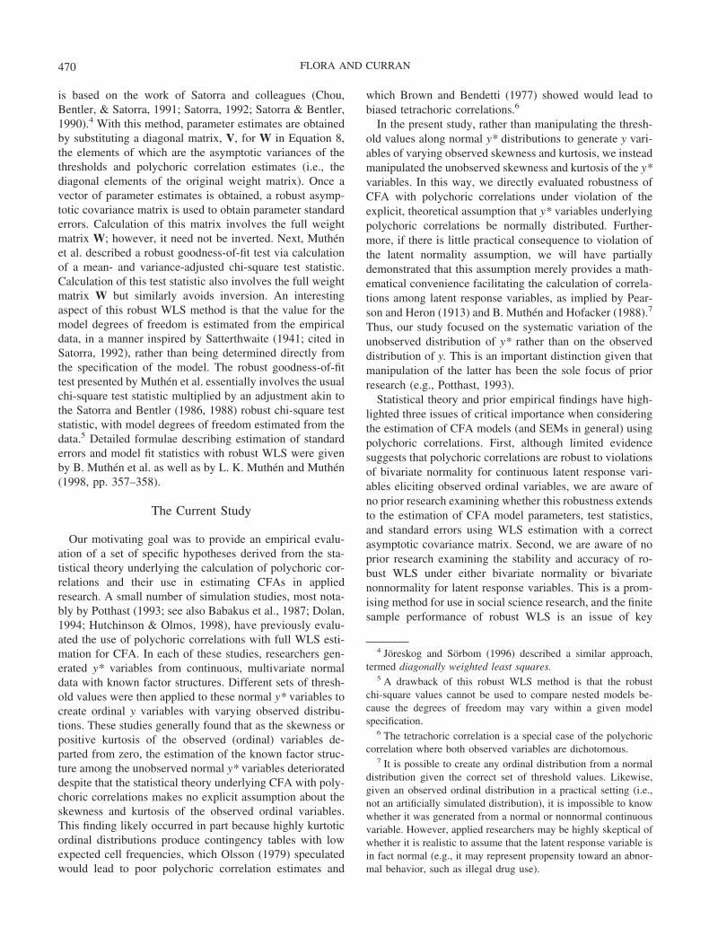
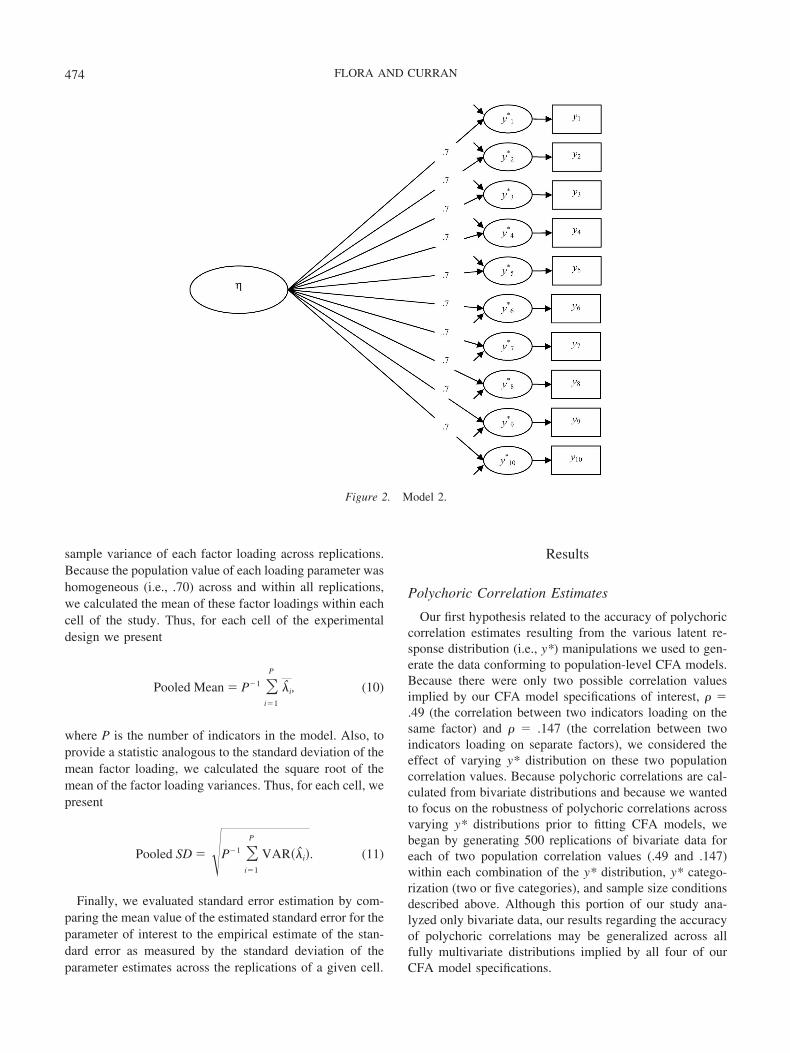
Each sample of multivariate data we generated had apopulation correlation matrix conforming to one of fourfactor model specifications that hold for the y* latent re-sponse variables. We selected these models to be represen-tative of CFA model specifications that might be encoun-tered in practice (e.g., models showing the relationshipsamong a set of Likert-type variables). Model 1 (see Figure1) consisted of a single factor measured by five ordinalindicators (i.e., observed y variables), each of which wasdetermined by a latent response variable (i.e., an unobservedy* variable), as described above. Model 2 (see Figure 2)consisted of a single factor measured by 10 indicators.Model 3 (see Figure 3) consisted of two correlated factorseach measured by five indicators. Finally, Model 4 (seeFigure 4) was identical to Model 3, except each factor wasmeasured by 10 indicators. As with Model 1, each of theordinal indicators for Models 2, 3, and 4 was determined byits own y* variable.

To facilitate interpretation, we defined the values of thepopulation parameters to be homogeneous across all fourmodel specifications. That is, within and across the models,all factor loadings were equal (�s � .70), and all unique-nesses were equal (�s � .51). Importantly, these loadingsrepresent the regression of the latent response variables (i.e.,the y* variables), and not the ordinal indicators, on thefactor. Models 3 and 4 included an interfactor correlation,which was set to �21 � .30 for both. All y* distributionswere standardized to have a mean of zero and standard

deviation equal to one, such that �i2 � �i � 1 for y*i. The

variances of the factors and of the uniquenesses were all setto equal one. Thus, the proposed models for the latentresponse variables were scale invariant (Cudeck, 1989, p.326), and it was valid to define the implied populationcovariance matrices for data simulation in terms ofcorrelations.

Data Generation and Analysis

For each combination of y* distribution and model spec-ification described above, we generated random samples offour different sizes: 100, 200, 500, and 1,000. We replicatedthe 5 (distributions) 4 (model specifications) 4 (samplesizes) 2 (number of categories) � 160 independent cellsof the study 500 times each, using EQS (Version 5.7b;Bentler, 1995) to generate all data for the study.10 For eachreplication, we fit the relevant population factor modelusing both full and robust WLS estimation as implemented

9 In the five-category condition, we used the Case 1 thresholdset from B. Muthen and Kaplan (1985), such that that categoriza-tion of a normal y* population distribution would result in anordinal y distribution with zero skewness and kurtosis. This samethreshold set was also applied to each nonnormal y*distribution.

10 We generated the raw data with the EQS implementation ofthe methods of Fleishman (1978), who presented formulae forsimulating univariate data with nonzero skewness and kurtosis,and Vale and Maurelli (1983), who extended Fleishman’s methodto allow simulation of multivariate data with known levels ofunivariate skewness and kurtosis and a known correlational struc-ture. To ensure that EQS properly created the data according to thedesired levels of skewness and kurtosis for the y* variables, wegenerated a set of continuous data conforming to Model 1 withN � 50,000 for each level of our manipulation of the y* distribu-tions. The values of univariate skewness and kurtosis calculatedfrom these large-sample data closely reflected the nominal popu-lation values. Previous studies have also successfully implementedthis method of data generation (e.g., Chou et al., 1991; Curran etal., 1996; Hu et al., 1992).

Table 1Skewness and Kurtosis of Univariate Latent Response (y*) Distributions and Five-CategoryOrdinal (y) Distributions

Condition

y* distribution y distribution

Skewness Kurtosis Skewness Kurtosis

Normal 0.00 0.00 0.02 �0.00Low skewness vs. low kurtosis 0.75 1.75 0.30 0.22Low skewness vs. moderate kurtosis 0.75 3.75 0.22 0.60Moderate skewness vs. low kurtosis 1.25 1.75 0.49 �0.06Moderate skewness vs. moderate kurtosis 1.25 3.75 0.47 0.39

Note. Skewness and kurtosis for y* distribution are nominal population values. Skewness and kurtosis for ydistribution are approximate population values estimated from simulated samples of size N � 50,000.


with Mplus (Version 2.01; L. K. Muthen & Muthen,1998).11

Study Outcomes

We began by examining rates of improper solutionsacross all study conditions. An improper solution was de-fined as a nonconverged solution or a solution that con-verged but resulted in one or more out-of-bound parameters(e.g., Heywood cases). Because the underlying purpose ofour study was to explicitly evaluate our proposed researchhypotheses under conditions commonly encountered in ap-plied research settings, we defined improper solutions to beinvalid empirical observations. To maximize the externalvalidity of our findings, we removed improper solutionsfrom subsequent analyses (see Chen, Bollen, Paxton, Cur-ran, & Kirby, 2001, for further discussion of this strategy).12

We considered three major outcomes of interest: the chi-square test statistics, parameter estimates (i.e., factor load-ings and factor correlations), and standard errors.

We examined the mean relative bias (RB; or percentagebias) of each outcome across all study conditions. Thegeneral form of this statistic is

RB � � �

� � 100, (9)

where is the estimated statistic (i.e., chi-square test statis-tic, CFA parameter estimate, or standard error) from a givenreplication, and is the relevant population parameter. Foreach outcome, we calculated the mean RB across replica-tions within a given condition. Consistent with prior simu-lation studies (e.g., Curran et al., 1996; Kaplan, 1989), weconsidered RB values less than 5% indicative of trivial bias,values between 5% and 10% indicative of moderate bias,and values greater than 10% indicative of substantial bias.

For the chi-square test statistics from full WLS estima-

tion, we calculated relative bias with respect to the degreesof freedom for each model specification, given that thisvalue reflects the expected value of a chi-square distribu-tion. With robust WLS estimation, the degrees of freedomfor the chi-square test statistic are estimated from the dataand, therefore, the expected value of the chi-square statisticvaries across samples within the same model specification.Thus, for each replication within a given condition, we usedthe estimated degrees of freedom to calculate the relativebias of the chi-square statistic elicited from the robustmethod. We then calculated the mean RB across sampleswithin a given study condition.

Because of the large number of factor loadings estimatedboth within and across replications, we examined the meanfactor loading values to summarize our results more effi-ciently. This strategy was appropriate given the homoge-neous values of factor loadings within each model specifi-cation. Specifically, within a given cell of the study, we firstcalculated the mean across replications of each individualloading parameter separately (e.g., for Model 1, we obtained�11, �21, �31, �41, and �51). In addition, we calculated the

11 Although we estimated our models using the commercialsoftware package, Mplus (L. K. Muthen & Muthen, 1998), equiv-alent results would be expected using any software package withthe capability for estimating polychoric correlations and theirasymptotic variances and covariances (e.g., PRELIS/LISREL:Joreskog & Sorbom, 1988, 1996; Mx: Neale, Boker, Xie, & Maes,2002).

12 Additional analyses reflected that the simultaneous inclusionof both proper and improper solutions resulted in modest changesin the summary statistics of the outcomes under study; however,the overall conclusions based only on the proper solutions remainsubstantively unchanged. Thus, there is no evidence suggestingthat the omission of the improper solutions poses a threat to eitherthe internal or the external validity of our study.

Figure 1. Model 1.

473ORDINAL CFA

sample variance of each factor loading across replications.Because the population value of each loading parameter washomogeneous (i.e., .70) across and within all replications,we calculated the mean of these factor loadings within eachcell of the study. Thus, for each cell of the experimentaldesign we present

Pooled Mean � P�1 �i�1

P

�i, (10)

where P is the number of indicators in the model. Also, toprovide a statistic analogous to the standard deviation of themean factor loading, we calculated the square root of themean of the factor loading variances. Thus, for each cell, wepresent

Pooled SD � �P�1 �i�1

P

VAR��i�. (11)

Finally, we evaluated standard error estimation by com-paring the mean value of the estimated standard error for theparameter of interest to the empirical estimate of the stan-dard error as measured by the standard deviation of theparameter estimates across the replications of a given cell.

Results

Polychoric Correlation Estimates

Our first hypothesis related to the accuracy of polychoriccorrelation estimates resulting from the various latent re-sponse distribution (i.e., y*) manipulations we used to gen-erate the data conforming to population-level CFA models.Because there were only two possible correlation valuesimplied by our CFA model specifications of interest, � �.49 (the correlation between two indicators loading on thesame factor) and � � .147 (the correlation between twoindicators loading on separate factors), we considered theeffect of varying y* distribution on these two populationcorrelation values. Because polychoric correlations are cal-culated from bivariate distributions and because we wantedto focus on the robustness of polychoric correlations acrossvarying y* distributions prior to fitting CFA models, webegan by generating 500 replications of bivariate data foreach of two population correlation values (.49 and .147)within each combination of the y* distribution, y* catego-rization (two or five categories), and sample size conditionsdescribed above. Although this portion of our study ana-lyzed only bivariate data, our results regarding the accuracyof polychoric correlations may be generalized across allfully multivariate distributions implied by all four of ourCFA model specifications.

Figure 2. Model 2.


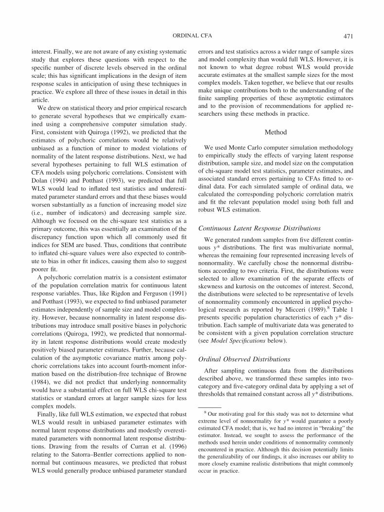
Table 2 summarizes results for the polychoric correlationsin the different study conditions. When the data were gen-erated from a bivariate normal y* distribution, the meanpolychoric correlation across replications was essentiallyequal to its population value (mean RB was less than 1% innearly every cell with underlying skewness � 0 and under-lying kurtosis � 0). The polychoric correlation estimatestended to become positively biased as a function of increas-ing nonnormality in the y* distributions; however, mean RBremained under 10% in almost all cells. For example, Figure5 presents box plots illustrating the distributions of poly-choric correlation estimates of � � .49 obtained with N �1,000 for the five-category condition. The figure reveals thatalthough the correlation estimates were frequently posi-tively biased, the center of these distributions did not departsubstantially from the population correlation value, evenwith y* nonnormality. Overall, correlation estimates of � �.147 rarely exceeded .16, and correlation estimates � � .49rarely exceeded .52. Finally, sample size did not have anyapparent effect on the accuracy of the polychoric correla-tions, although there was a tendency for correlations calcu-lated from two-category data to be slightly more biased thanthose calculated from five-category data.

Theory would not predict that varying the thresholdsacross observed variables would influence our findings de-scribed above. However, to examine this possibility empir-ically, we generated additional bivariate y* data from thecondition with skewness � 1.25 and kurtosis � 3.75. We

applied the threshold values to y*1 to create a five-categoryy1 distribution with the same skewness and kurtosis valuesas given in the moderate versus moderate case in Table 1,but different threshold values were applied to y*2 resulting ina five-category population distribution for y2 with skew-ness � �2.36 and kurtosis � 5.15. When samples of sizeN � 1,000 (again with 500 replications) were generatedfrom this bivariate population distribution with true corre-lation � � .49, the mean polychoric correlation estimate was0.51 (SD � 0.04), with mean RB of 3.21%. Thus, this resultshows that polychoric correlations remain only slightly bi-ased when markedly different sets of threshold values areapplied to the two correlated y* variables generating theobserved ordinal variables.

Finally, to evaluate the effect of extremely nonnormaldistributions, we generated data from correlated y* vari-ables defined by drastically nonnormal distributions (skew-ness � 5, kurtosis � 50) and applied the same sets ofthresholds as above to create five-category ordinal variables(resulting in skewness � 1.68 and kurtosis � 7.01 for y1

and y2 when the same set of thresholds was applied to bothy*1 and y*2 and skewness � �7.86 and kurtosis � 64.63 fory2 when different thresholds were applied to y*2). We againgenerated 500 replications with N � 1,000 from each ofthese bivariate population distributions. With a true corre-lation of � � .49, the mean polychoric correlation estimatewas 0.65 (SD � 0.04), with mean RB of 31.43% whenthresholds were equal across y*1 and y*2. When the set of

Figure 3. Model 3.

475ORDINAL CFA

thresholds varied across y*1 and y*2, the mean polychoriccorrelation was 0.64 (SD � 0.09), with mean RB of 32.21%.Thus, polychoric correlations do not appear to be robust toextreme violations of the latent normality assumption, and

this result does not seem to vary substantially when differ-ent sets of thresholds are applied to y* variables.

In sum, consistent with Quiroga (1992), our empiricalresults suggest that polychoric correlations provide unbi-

Figure 4. Model 4.


ased estimates of the correlations among normal and mod-erately nonnormal latent response variables. We did findevidence that severely nonnormal distributions led to sub-stantial distortions in the estimation of the polychoric cor-relation structure and, given this distortion, we did notpursue the fitting of subsequent CFAs further. However, therobustness of polychoric correlations to minor-to-moderateviolations of normality is a necessary but, quite importantly,not a sufficient condition to establish whether CFA modelsfor latent response variables can be accurately fitted withpolychoric correlation matrices. Thus, we next turn to theestimation of our CFA models using polychoric correlationsestimating the relationships among latent response variablesof varying distribution.

Estimation of CFA Models

Rates of improper solutions. The rates of improper andnonconverged solutions obtained with full WLS estimationare given in Table 3. With N � 100, full WLS did notproduce any solutions for Model 4, the 20-indicator model(due to noninvertible weight matrices). In general, the ratesof improper solutions were greater in the two-categoryversus five-category condition. For the two 10-indicatormodels (Models 2 and 3), two-category data produced highrates of improper solutions with N � 100, whereas the rateswere near zero in the five-category condition. Also, nearly100% of replications of Model 4 (the 20-indicator model)

were improper in the two-category condition where N �200, whereas the corresponding rates in the five-categorycondition were only around 30%. Although the rates ofimproper solution obtained with full WLS varied somewhatacross different y* distributions, this variation did not ap-pear to be systematically associated with degree of nonnor-mality in y*. At the two largest sample sizes (N � 500 andN � 1,000), full WLS estimation converged to propersolutions of all four models across 100% of replications.

In sum, there were modest differences evident in theconvergence rates for the two-category and five-categoryconditions. However, extensive analyses (not fully reportedhere) revealed that the empirical results for the chi-squaretest statistics, parameter estimates, and standard errors werenearly identical for these two conditions across all experi-mental conditions. Given this equivalence, we present thefindings related to the five-category condition to retainscope and maximize focus.13

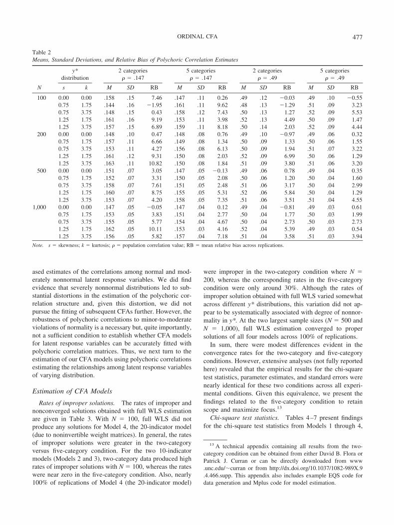
Chi-square test statistics. Tables 4–7 present findingsfor the chi-square test statistics from Models 1 through 4,

13 A technical appendix containing all results from the two-category condition can be obtained from either David B. Flora orPatrick J. Curran or can be directly downloaded from www.unc.edu/�curran or from http://dx.doi.org/10.1037/1082-989X.9.4.466.supp. This appendix also includes example EQS code fordata generation and Mplus code for model estimation.

Table 2Means, Standard Deviations, and Relative Bias of Polychoric Correlation Estimates

N

y*distribution

2 categories� � .147




s k M SD RB M SD RB M SD RB M SD RB

100 0.00 0.00 .158 .15 7.46 .147 .11 0.26 .49 .12 �0.03 .49 .10 �0.550.75 1.75 .144 .16 �1.95 .161 .11 9.62 .48 .13 �1.29 .51 .09 3.230.75 3.75 .148 .15 0.43 .158 .12 7.43 .50 .13 1.27 .52 .09 5.531.25 1.75 .161 .16 9.19 .153 .11 3.98 .52 .13 4.49 .50 .09 1.471.25 3.75 .157 .15 6.89 .159 .11 8.18 .50 .14 2.03 .52 .09 4.44

200 0.00 0.00 .148 .10 0.47 .148 .08 0.76 .49 .10 �0.97 .49 .06 0.320.75 1.75 .157 .11 6.66 .149 .08 1.34 .50 .09 1.33 .50 .06 1.550.75 3.75 .153 .11 4.27 .156 .08 6.13 .50 .09 1.94 .51 .07 3.221.25 1.75 .161 .12 9.31 .150 .08 2.03 .52 .09 6.99 .50 .06 1.291.25 3.75 .163 .11 10.82 .150 .08 1.84 .51 .09 3.80 .51 .06 3.20

500 0.00 0.00 .151 .07 3.05 .147 .05 �0.13 .49 .06 0.78 .49 .04 0.350.75 1.75 .152 .07 3.31 .150 .05 2.08 .50 .06 1.20 .50 .04 1.600.75 3.75 .158 .07 7.61 .151 .05 2.48 .51 .06 3.17 .50 .04 2.991.25 1.75 .160 .07 8.75 .155 .05 5.31 .52 .06 5.84 .50 .04 1.291.25 3.75 .153 .07 4.20 .158 .05 7.35 .51 .06 3.51 .51 .04 4.55

1,000 0.00 0.00 .147 .05 �0.05 .147 .04 0.12 .49 .04 �0.81 .49 .03 0.610.75 1.75 .153 .05 3.83 .151 .04 2.77 .50 .04 1.77 .50 .03 1.990.75 3.75 .155 .05 5.77 .154 .04 4.67 .50 .04 2.73 .50 .03 2.731.25 1.75 .162 .05 10.11 .153 .03 4.16 .52 .04 5.39 .49 .03 0.541.25 3.75 .156 .05 5.82 .157 .04 7.18 .51 .04 3.58 .51 .03 3.94

Note. s � skewness; k � kurtosis; � � population correlation value; RB � mean relative bias across replications.

477ORDINAL CFA

respectively. Recall that with full WLS, the model degreesof freedom, and hence the expected value of the chi-squaretest statistic, is determined directly from model specifica-tion, whereas with robust WLS, the model degrees of free-dom is estimated in part from characteristics of the data andvaries across samples. Thus, although we present the across-replication mean and standard deviation of chi-square sta-tistics obtained with full WLS, we do not present the across-replication mean and standard deviation of chi-squarevalues obtained with robust WLS because the expectedvalue of these statistics varies across replications within agiven cell. For both methods of estimation, we present themean RB of the chi-square test statistics and the observedType I error rate (using � � .05) for each cell. With robustWLS, we calculated chi-square percentage bias for eachreplication relative to its observed degrees of freedom andthen computed the mean percentages across replications toestimate RB.

Both the chi-square test statistics and their standard de-viations tend to be positively biased across all cells of the

study, particularly with full WLS estimation. This biasincreases as a function of increasing model complexity. Forexample, full WLS chi-square statistics from Model 1 haveRB values ranging from 0.02% to 7.63% with N � 500,whereas full WLS chi-square values from Model 4 showmuch greater inflation, as RB is approximately 65% withN � 500. Comparison of the findings for Model 2 with thosefor Model 3 reveals that the bias in chi-square statistics isaffected not only by the number of indicators for a modelbut also by model complexity. Model 2 and Model 3 bothhave 10 indicators, but in Model 3 the indicators measuretwo correlated factors, whereas the indicators for Model 2measure a single dimension. Because of this added modelcomplexity, the chi-square statistics for Model 3 are slightlymore inflated than those for Model 2.

The effect of sample size on the inflation in chi-squaretest values varies substantially with model specification.Within each of the four models, the chi-square RB de-creases as sample size increases, but this effect is morepronounced for larger models. In addition, there appears

Figure 5. Distribution of polychoric correlation estimates obtained with N � 1,000 (horizontal linerepresents population correlation value). s � skewness; k � kurtosis.


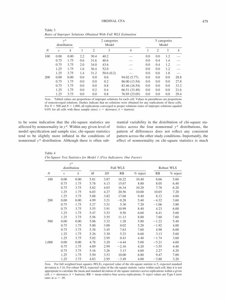
to be some indication that the chi-square statistics areaffected by nonnormality in y*. Within any given level ofmodel specification and sample size, chi-square statisticstend to be slightly more inflated in the conditions ofnonnormal y* distribution. Although there is often sub-

stantial variability in the distribution of chi-square sta-tistics across the four nonnormal y* distributions, thepattern of differences does not reflect any consistentpattern across the other study conditions. Importantly, theeffect of nonnormality on chi-square statistics is much

Table 3Rates of Improper Solutions Obtained With Full WLS Estimation

N

y*distribution

2 categoriesModel

5 categoriesModel

s k 1 2 3 4 1 2 3 4

100 0.00 0.00 2.2 30.4 40.2 — 0.0 0.0 1.2 —0.75 1.75 0.6 31.6 40.6 — 0.0 0.4 1.4 —0.75 3.75 2.0 34.0 43.6 — 0.0 0.4 1.2 —1.25 1.75 1.6 36.4 52.0 — 0.0 0.0 1.2 —1.25 3.75 1.4 31.2 50.6 (0.2) — 0.0 0.6 1.8 —

200 0.00 0.00 0.0 0.0 0.6 94.02 (5.77) 0.0 0.0 0.0 28.80.75 1.75 0.0 0.0 0.2 86.00 (13.54) 0.0 0.0 0.0 27.80.75 3.75 0.0 0.0 0.8 83.46 (16.54) 0.0 0.0 0.0 33.21.25 1.75 0.0 0.2 0.4 66.51 (33.49) 0.0 0.0 0.0 21.61.25 3.75 0.0 0.0 0.8 76.95 (23.05) 0.0 0.0 0.0 29.4

Note. Tabled values are proportions of improper solutions for each cell. Values in parentheses are proportionsof nonconverged solutions. Dashes indicate that no solutions were obtained for any replications of these cells.For N � 500 and N � 1,000, all replications converged to proper solutions (rates of improper solutions equaled0.0% for all cells with these sample sizes). s � skewness; k � kurtosis.

Table 4Chi-Square Test Statistics for Model 1 (Five Indicators, One Factor)

N

y*distribution Full WLS Robust WLS

s k M SD RB % reject RB % reject

100 0.00 0.00 5.81 3.87 16.22 10.40 8.66 5.600.75 1.75 5.78 4.13 15.67 8.80 8.05 6.400.75 3.75 5.82 4.03 16.34 10.20 7.78 6.201.25 1.75 6.03 4.27 20.56 10.00 10.65 7.201.25 3.75 5.88 3.82 17.68 9.40 8.12 4.60

200 0.00 0.00 4.99 3.21 �0.28 5.40 �4.32 3.600.75 1.75 5.27 3.51 5.30 7.20 �1.06 3.800.75 3.75 5.55 3.91 10.99 8.40 4.23 6.001.25 1.75 5.47 3.53 9.50 6.60 6.41 5.601.25 3.75 5.56 3.55 11.13 8.00 7.60 7.60

500 0.00 0.00 5.06 3.32 1.28 5.80 �1.22 5.400.75 1.75 5.00 3.00 0.02 5.20 �1.92 4.000.75 3.75 5.38 3.45 7.63 7.60 4.98 6.001.25 1.75 5.26 3.30 5.23 6.60 3.13 5.601.25 3.75 5.02 2.95 0.43 4.40 �1.74 3.60

1,000 0.00 0.00 4.78 3.20 �4.44 5.00 �5.21 4.600.75 1.75 4.89 2.99 �2.16 4.20 �3.55 4.400.75 3.75 5.16 3.26 3.13 4.60 2.27 4.201.25 1.75 5.50 3.53 10.00 6.80 9.47 7.001.25 3.75 4.83 2.95 �3.49 4.00 �3.88 3.20

Note. For full weighted least squares (WLS), expected value of the chi-square statistic is 5; expected standarddeviation is 3.16. For robust WLS, expected value of the chi-square statistic varies within each cell, thus it is notappropriate to calculate the mean and standard deviation of chi-square statistics across replications within a givencell. s � skewness; k � kurtosis; RB � mean relative bias across replications; % reject values are Type I errorrates at � � .05.

479ORDINAL CFA

less pronounced than are the effects of model specifica-tion and sample size.

In general, the robust WLS chi-square statistics are in-flated across most cells of the study, although typically byless than 10% of their population values (except with N �100, where RB values tend to be between 10% and 20%).This positive bias is drastically smaller with robust WLSestimation relative to full WLS estimation, especially forthe larger models. Furthermore, the influence of sample sizeon the chi-square test statistics appears to be much greaterwith full WLS than it does with robust WLS. Figure 6illustrates Type I error rates for the model chi-square test bysample size for Models 1 and 3, as estimated with both fullWLS and robust WLS. The figure reflects that for smallmodels (i.e., the five-indicator Model 1), both methods ofestimation lead to Type I error rates close to the nominalalpha level of .05 across all four sample sizes. The figurealso shows that for a more complex model (i.e., Model 3,where 10 indicators represent two factors), full WLS esti-mation produces vastly inflated Type I error rates withsamples of size less than N � 1,000, whereas the robustWLS method continues to produce Type I error rates closeto the nominal alpha level across all sample sizes. Finally,there does not appear to be any consistent tendency for

robust WLS chi-square values to be more biased undernonnormal y*.

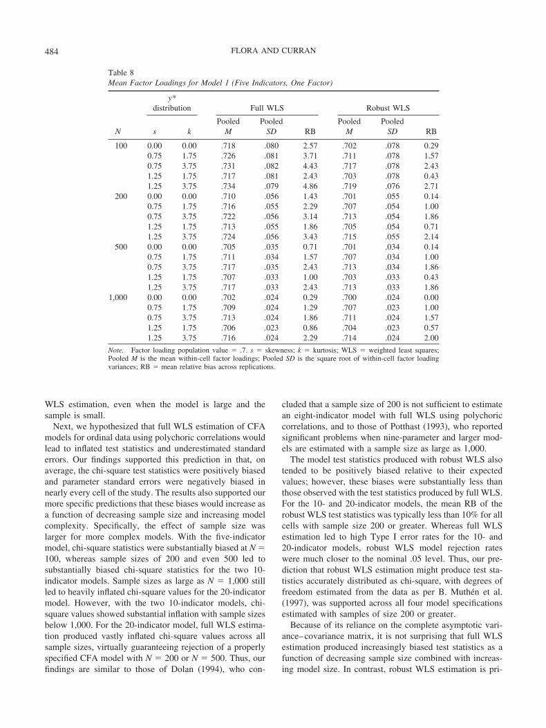
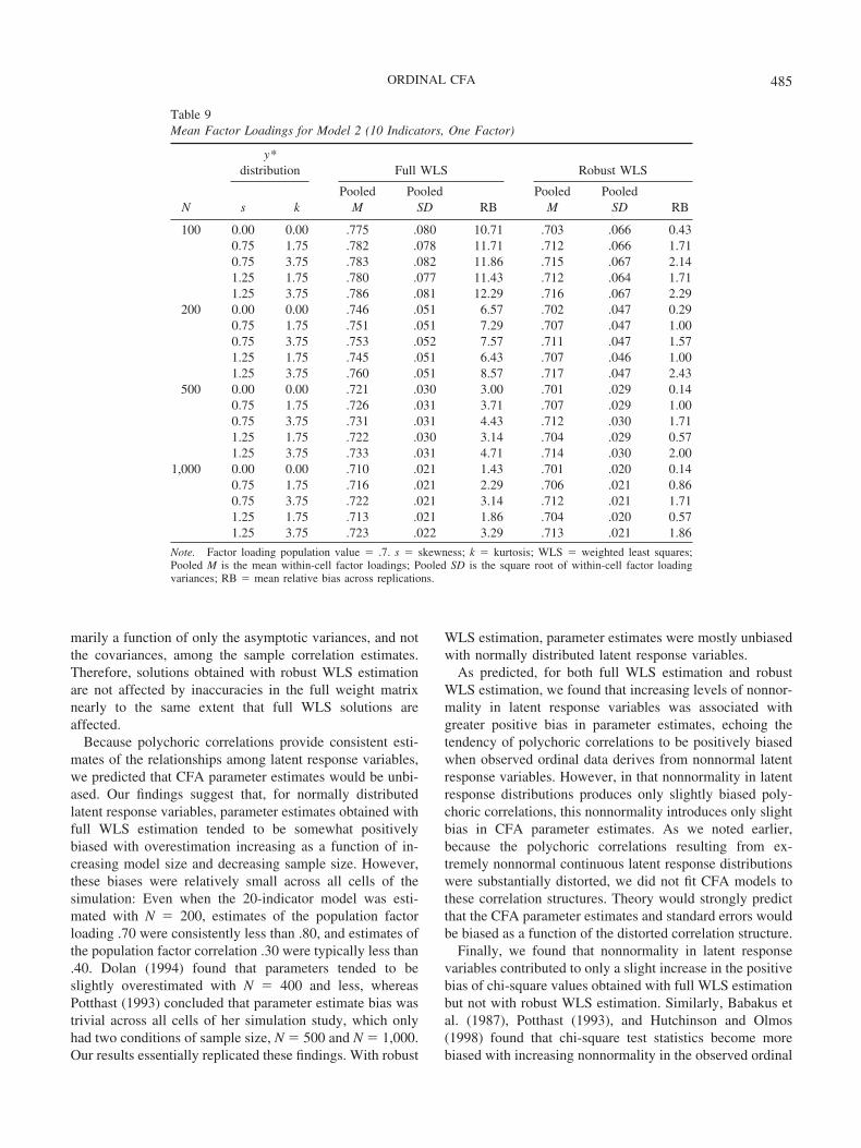
Parameter estimates. Tables 8–11 present findings per-taining to the parameter estimates (i.e., factor loadings andinterfactor correlations) obtained for Models 1, 2, 3, and 4,respectively. On average, the parameters are overestimatedacross all conditions, and this positive bias increases withincreasing model size. However, the overall bias in param-eter estimation is notably smaller with robust WLS than it iswith full WLS, especially for larger models and smallersample sizes. In general, the bias in parameter estimatesobtained with robust WLS is consistently trivial (i.e., lessthan 5%, with the exception of estimates of factor correla-tions with N � 100 and 200, where RB is trivial to mod-erate, or less than 10%). Even with full WLS estimation, theparameter overestimation is typically small, rarely leadingto parameter estimates greater than the corresponding pop-ulation value by more than .1 in the correlation metric.Whereas the overestimation of parameters with full WLSincreases as a function of increasing number of indicatorsfor the model, there is no such effect of model size onparameter estimation with robust WLS. Furthermore, pa-rameter overestimation with full WLS improves as a func-tion of increasing sample size, particularly with larger mod-

Table 5Chi-Square Test Statistics for Model 2 (10 Indicators, One Factor)

N



100 0.00 0.00 59.68 19.94 70.50 63.80 8.42 6.400.75 1.75 61.33 20.39 75.21 66.06 8.65 7.400.75 3.75 63.14 21.49 80.41 70.68 10.17 8.001.25 1.75 64.51 19.28 84.32 77.60 16.10 12.401.25 3.75 60.19 18.69 71.99 70.42 7.68 5.00

200 0.00 0.00 44.55 12.88 27.28 28.60 4.25 5.600.75 1.75 45.14 12.73 28.98 32.00 4.05 3.800.75 3.75 45.40 12.19 29.70 33.60 4.46 6.401.25 1.75 47.88 13.86 36.81 38.80 9.15 10.201.25 3.75 45.37 12.52 29.64 33.20 5.34 4.00

500 0.00 0.00 38.53 10.11 10.08 13.80 1.85 6.000.75 1.75 38.13 9.68 8.95 12.80 0.11 3.600.75 3.75 38.61 9.79 10.31 13.00 1.02 3.801.25 1.75 41.01 10.23 17.23 18.60 6.19 7.801.25 3.75 38.30 9.90 9.42 11.40 1.62 6.20

1,000 0.00 0.00 36.52 9.31 4.35 8.40 �0.15 5.000.75 1.75 36.54 9.51 4.39 9.40 �0.22 6.000.75 3.75 36.77 9.46 5.06 9.40 0.13 5.801.25 1.75 39.00 9.78 11.42 14.00 6.44 9.201.25 3.75 36.98 9.38 5.67 8.60 1.59 6.00



els. But with robust WLS, the effect of sample size onparameter estimation is quite small.

Parameter estimates (both factor loadings and factor cor-relations) seem to be affected by nonnormality in the y*variables, although this effect is small. Across all cells, theparameter estimates are positively biased, even with normaly*, and this parameter overestimation increases with greaternonnormality in y*. For example, using full WLS estima-tion, the mean RB of factor loadings when Model 1 isestimated from normally distributed y* variables is 2.57%with N � 100 and 0.29% with N � 1,000, yet when thesame model is estimated from y* variables with univariateskewness � 1.25 and univariate kurtosis � 3.75, the meanRB of factor loadings is 4.86% with N � 100 and 2.29%with N � 1,000. Overall, this small effect of y* nonnormal-ity on parameter estimation was found with both full androbust WLS estimation.

Standard errors. The conditions leading to greater biasin the standard errors were nearly identical to those that ledto greater bias in chi-square test statistics, thus we do notpresent detailed results pertaining to standard error estima-tion.14 Across all study conditions, the standard errors wereconsistently negatively biased relative to the standard devi-ation of the relevant parameter sampling distribution ob-tained empirically across replications. Specifically, standard

errors were more biased as a function of increasing modelsize and decreasing sample size but were not systematicallyaffected by y* nonnormality. Under full WLS estimation atN � 1,000, the mean factor loading standard error RBranges from around �2.5% to �1% across replications ofModel 1, from around �9% to �5% across replications ofModels 2 and 3, and from around �25% to �22% acrossreplications of Model 4. Although the robust WLS approachalso frequently produced negatively biased standard errors,these biases were much smaller than the standard error biasproduced with full WLS estimation. Using the robust WLSmethod with N � 1,000, the mean factor loading standarderror RB ranges from around �1% to 1% across replica-tions of Model 1, from around �3% to 1% across replica-tions of Models 2 and 3, and from around �3% to �1%across replications of Model 4.

14 Complete results pertaining to standard error estimates arealso included in the technical appendix that can be obtained fromeither David B. Flora or Patrick J. Curran or downloaded fromwww.unc.edu/�curran or from http://dx.doi.org/10.1037/1082-989X.9.4.466.supp.

Table 6Chi-Square Test Statistics for Model 3 (10 Indicators, Two Correlated Factors)

N



100 0.00 0.00 65.25 22.94 91.90 74.29 15.03 12.200.75 1.75 65.95 23.71 93.96 73.63 16.85 12.400.75 3.75 67.49 22.22 98.51 81.38 14.46 12.001.25 1.75 65.78 22.92 93.48 75.51 16.76 12.201.25 3.75 65.44 22.54 92.46 77.80 15.10 10.80

200 0.00 0.00 45.98 13.59 35.23 37.80 5.47 6.600.75 1.75 46.34 15.03 36.29 39.40 6.53 7.600.75 3.75 46.90 13.79 37.94 40.40 5.49 7.801.25 1.75 47.73 14.19 40.38 42.40 10.20 8.601.25 3.75 46.09 14.06 35.55 38.80 6.51 8.60

500 0.00 0.00 38.14 10.17 12.19 15.60 1.40 5.000.75 1.75 38.97 10.06 14.62 16.60 3.33 6.600.75 3.75 38.46 9.79 13.10 15.60 3.10 7.801.25 1.75 40.16 11.12 18.13 19.00 6.93 8.201.25 3.75 38.77 10.65 14.04 15.20 3.65 7.20

1,000 0.00 0.00 36.04 8.88 6.00 9.60 1.36 5.600.75 1.75 36.29 9.28 6.74 10.20 1.65 5.800.75 3.75 36.11 8.80 6.21 8.20 �0.19 3.801.25 1.75 37.24 9.00 9.54 10.60 2.75 5.601.25 3.75 35.69 9.38 4.97 8.60 �1.68 3.60


481ORDINAL CFA

Discussion

We used a comprehensive simulation study to empiricallytest our set of theoretically generated research hypothesespertaining to the performance of CFA for ordinal data withpolychoric correlations using both full WLS (as perBrowne, 1984, and B. Muthen, 1983, 1984) and robustWLS (as per Muthen et al., 1997) estimation. The results ofour study provided support for each of our proposedhypotheses.

First, as predicted, we replicated Quiroga’s (1992) find-ings that polychoric correlations among ordinal variablesaccurately estimated the bivariate relations among normallydistributed latent response variables and that modest viola-tion of normality for latent response variables of a degreethat might be expected in applied research leads to onlyslightly biased estimates of polychoric correlations. Bothour results and Quiroga’s suggest that this finding occursregardless of whether the same set of threshold values isapplied to both latent response variables leading to theobserved ordinal variables. A thorough examination of theeffects of differing thresholds and level of skewness acrossthe two variables on polychoric correlation estimates is

beyond the scope of our study. However, we note thatQuiroga found that polychoric correlation estimates re-mained accurate when the ordinal variables had differingthresholds or skewness of opposite sign. Specifically, al-though increasing levels of nonnormality tended to produceincreasingly positively biased correlation estimates, thesebiases remained quite small and were typically less than .03in the correlation metric. Furthermore, we found that vari-ability in polychoric correlations was not affected by non-normality and that sample size had no effect on the meanpolychoric correlation estimates across cells.

These results likely occurred because nonnormality in thelatent response variables, in combination with the thresholdvalues used to categorize the data, did not produce contin-gency tables with low expected cell frequencies (see Brown& Bendetti, 1977; Olsson, 1979). Because our results indi-cated that the polychoric correlations accurately recoveredthe correlations among the unobserved y* variables evenunder modest violation of the normality assumption, weproceeded to examine the adequacy of fitting CFA modelsto these correlation structures.

As we described earlier, it has been analytically demon-strated that when CFA models are fitted using observed

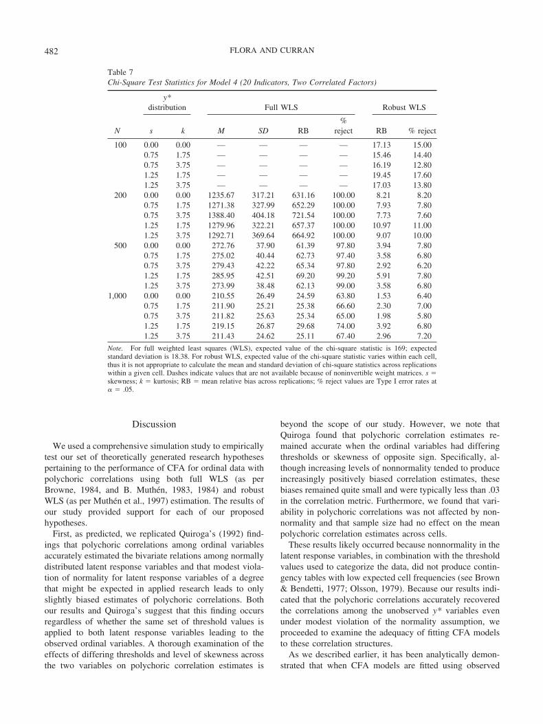
Table 7Chi-Square Test Statistics for Model 4 (20 Indicators, Two Correlated Factors)

N


s k M SD RB%

reject RB % reject

100 0.00 0.00 — — — — 17.13 15.000.75 1.75 — — — — 15.46 14.400.75 3.75 — — — — 16.19 12.801.25 1.75 — — — — 19.45 17.601.25 3.75 — — — — 17.03 13.80

200 0.00 0.00 1235.67 317.21 631.16 100.00 8.21 8.200.75 1.75 1271.38 327.99 652.29 100.00 7.93 7.800.75 3.75 1388.40 404.18 721.54 100.00 7.73 7.601.25 1.75 1279.96 322.21 657.37 100.00 10.97 11.001.25 3.75 1292.71 369.64 664.92 100.00 9.07 10.00

500 0.00 0.00 272.76 37.90 61.39 97.80 3.94 7.800.75 1.75 275.02 40.44 62.73 97.40 3.58 6.800.75 3.75 279.43 42.22 65.34 97.80 2.92 6.201.25 1.75 285.95 42.51 69.20 99.20 5.91 7.801.25 3.75 273.99 38.48 62.13 99.00 3.58 6.80

1,000 0.00 0.00 210.55 26.49 24.59 63.80 1.53 6.400.75 1.75 211.90 25.21 25.38 66.60 2.30 7.000.75 3.75 211.82 25.63 25.34 65.00 1.98 5.801.25 1.75 219.15 26.87 29.68 74.00 3.92 6.801.25 3.75 211.43 24.62 25.11 67.40 2.96 7.20

Note. For full weighted least squares (WLS), expected value of the chi-square statistic is 169; expectedstandard deviation is 18.38. For robust WLS, expected value of the chi-square statistic varies within each cell,thus it is not appropriate to calculate the mean and standard deviation of chi-square statistics across replicationswithin a given cell. Dashes indicate values that are not available because of noninvertible weight matrices. s �skewness; k � kurtosis; RB � mean relative bias across replications; % reject values are Type I error rates at� � .05.


polychoric correlation matrices, full WLS estimation pro-duces asymptotically correct chi-square tests of model fitand parameter standard errors (e.g., B. Muthen, 1983, 1984;B. O. Muthen & Satorra, 1995). However, in practice, theuse of full WLS is often problematic, especially whenmodels with a large number of indicators are estimated withsample sizes typically encountered in social science re-search. In our study, we found that when the 20-indicatormodel (Model 4) was estimated using N � 100, the esti-mated asymptotic covariance matrix W was consistentlynonpositive definite and could not be inverted for any of thereplications. Thus, not a single solution across all replica-tions was obtained in this situation using full WLS estima-tion. This finding is consistent with Browne’s (1984) obser-vation that this method of estimation “will tend to becomeinfeasible” as the number of variables approaches p � 20 (p.73) and Joreskog & Sorbom’s (1996) recommendation thata minimum sample size be attained for estimation of W.When Model 4 was estimated with samples of size N � 200,W was usually invertible, but the full WLS fitting functionfrequently failed to converge to a proper CFA solution.

However, the overall rates of nonconvergence and im-

proper solutions obtained with full WLS in the present studyare less than those found in simulation studies applying fullWLS to continuously distributed data (e.g., Curran et al.,1996). Nonetheless, other studies applying full WLS esti-mation to the analysis of polychoric correlations have foundrates of nonconvergence and improper solutions similar tothose reported here: Neither Dolan (1994) nor Potthast(1993) obtained nonpositive definite weight matrices orimproper solutions for any replications of their respectivestudies, which analyzed samples of size 200 and greater,whereas Babakus et al. (1987) obtained high rates of non-convergence and improper solutions only with samples of100.

One advantage of the robust WLS method relative to fullWLS is that sample solutions for the CFA model can still beobtained with robust WLS estimation even when the weightmatrix is nonpositive definite. Thus, robust WLS estimationsuccessfully obtained solutions to Model 4 with N � 100,whereas full WLS did not. Furthermore, our findings showthat the likelihood of obtaining an improper solution orencountering convergence difficulty is near zero with robust

Figure 6. Type I error rates with nominal alpha level � .05 for chi-square test of model fit bysample size for Model 1 (5 indicators of one factor) and Model 3 (10 indicators of two factors).WLS � weighted least squares.

483ORDINAL CFA

WLS estimation, even when the model is large and thesample is small.

Next, we hypothesized that full WLS estimation of CFAmodels for ordinal data using polychoric correlations wouldlead to inflated test statistics and underestimated standarderrors. Our findings supported this prediction in that, onaverage, the chi-square test statistics were positively biasedand parameter standard errors were negatively biased innearly every cell of the study. The results also supported ourmore specific predictions that these biases would increase asa function of decreasing sample size and increasing modelcomplexity. Specifically, the effect of sample size waslarger for more complex models. With the five-indicatormodel, chi-square statistics were substantially biased at N �100, whereas sample sizes of 200 and even 500 led tosubstantially biased chi-square statistics for the two 10-indicator models. Sample sizes as large as N � 1,000 stillled to heavily inflated chi-square values for the 20-indicatormodel. However, with the two 10-indicator models, chi-square values showed substantial inflation with sample sizesbelow 1,000. For the 20-indicator model, full WLS estima-tion produced vastly inflated chi-square values across allsample sizes, virtually guaranteeing rejection of a properlyspecified CFA model with N � 200 or N � 500. Thus, ourfindings are similar to those of Dolan (1994), who con-

cluded that a sample size of 200 is not sufficient to estimatean eight-indicator model with full WLS using polychoriccorrelations, and to those of Potthast (1993), who reportedsignificant problems when nine-parameter and larger mod-els are estimated with a sample size as large as 1,000.

The model test statistics produced with robust WLS alsotended to be positively biased relative to their expectedvalues; however, these biases were substantially less thanthose observed with the test statistics produced by full WLS.For the 10- and 20-indicator models, the mean RB of therobust WLS test statistics was typically less than 10% for allcells with sample size 200 or greater. Whereas full WLSestimation led to high Type I error rates for the 10- and20-indicator models, robust WLS model rejection rateswere much closer to the nominal .05 level. Thus, our pre-diction that robust WLS estimation might produce test sta-tistics accurately distributed as chi-square, with degrees offreedom estimated from the data as per B. Muthen et al.(1997), was supported across all four model specificationsestimated with samples of size 200 or greater.

Because of its reliance on the complete asymptotic vari-ance–covariance matrix, it is not surprising that full WLSestimation produced increasingly biased test statistics as afunction of decreasing sample size combined with increas-ing model size. In contrast, robust WLS estimation is pri-

Table 8Mean Factor Loadings for Model 1 (Five Indicators, One Factor)

N


s kPooled

MPooled

SD RBPooled

MPooled

SD RB

100 0.00 0.00 .718 .080 2.57 .702 .078 0.290.75 1.75 .726 .081 3.71 .711 .078 1.570.75 3.75 .731 .082 4.43 .717 .078 2.431.25 1.75 .717 .081 2.43 .703 .078 0.431.25 3.75 .734 .079 4.86 .719 .076 2.71

200 0.00 0.00 .710 .056 1.43 .701 .055 0.140.75 1.75 .716 .055 2.29 .707 .054 1.000.75 3.75 .722 .056 3.14 .713 .054 1.861.25 1.75 .713 .055 1.86 .705 .054 0.711.25 3.75 .724 .056 3.43 .715 .055 2.14

500 0.00 0.00 .705 .035 0.71 .701 .034 0.140.75 1.75 .711 .034 1.57 .707 .034 1.000.75 3.75 .717 .035 2.43 .713 .034 1.861.25 1.75 .707 .033 1.00 .703 .033 0.431.25 3.75 .717 .033 2.43 .713 .033 1.86

1,000 0.00 0.00 .702 .024 0.29 .700 .024 0.000.75 1.75 .709 .024 1.29 .707 .023 1.000.75 3.75 .713 .024 1.86 .711 .024 1.571.25 1.75 .706 .023 0.86 .704 .023 0.571.25 3.75 .716 .024 2.29 .714 .024 2.00

Note. Factor loading population value � .7. s � skewness; k � kurtosis; WLS � weighted least squares;Pooled M is the mean within-cell factor loadings; Pooled SD is the square root of within-cell factor loadingvariances; RB � mean relative bias across replications.


marily a function of only the asymptotic variances, and notthe covariances, among the sample correlation estimates.Therefore, solutions obtained with robust WLS estimationare not affected by inaccuracies in the full weight matrixnearly to the same extent that full WLS solutions areaffected.

Because polychoric correlations provide consistent esti-mates of the relationships among latent response variables,we predicted that CFA parameter estimates would be unbi-ased. Our findings suggest that, for normally distributedlatent response variables, parameter estimates obtained withfull WLS estimation tended to be somewhat positivelybiased with overestimation increasing as a function of in-creasing model size and decreasing sample size. However,these biases were relatively small across all cells of thesimulation: Even when the 20-indicator model was esti-mated with N � 200, estimates of the population factorloading .70 were consistently less than .80, and estimates ofthe population factor correlation .30 were typically less than.40. Dolan (1994) found that parameters tended to beslightly overestimated with N � 400 and less, whereasPotthast (1993) concluded that parameter estimate bias wastrivial across all cells of her simulation study, which onlyhad two conditions of sample size, N � 500 and N � 1,000.Our results essentially replicated these findings. With robust

WLS estimation, parameter estimates were mostly unbiasedwith normally distributed latent response variables.

As predicted, for both full WLS estimation and robustWLS estimation, we found that increasing levels of nonnor-mality in latent response variables was associated withgreater positive bias in parameter estimates, echoing thetendency of polychoric correlations to be positively biasedwhen observed ordinal data derives from nonnormal latentresponse variables. However, in that nonnormality in latentresponse distributions produces only slightly biased poly-choric correlations, this nonnormality introduces only slightbias in CFA parameter estimates. As we noted earlier,because the polychoric correlations resulting from ex-tremely nonnormal continuous latent response distributionswere substantially distorted, we did not fit CFA models tothese correlation structures. Theory would strongly predictthat the CFA parameter estimates and standard errors wouldbe biased as a function of the distorted correlation structure.

Finally, we found that nonnormality in latent responsevariables contributed to only a slight increase in the positivebias of chi-square values obtained with full WLS estimationbut not with robust WLS estimation. Similarly, Babakus etal. (1987), Potthast (1993), and Hutchinson and Olmos(1998) found that chi-square test statistics become morebiased with increasing nonnormality in the observed ordinal

Table 9Mean Factor Loadings for Model 2 (10 Indicators, One Factor)

N


s kPooled

MPooled

SD RBPooled

MPooled

SD RB

100 0.00 0.00 .775 .080 10.71 .703 .066 0.430.75 1.75 .782 .078 11.71 .712 .066 1.710.75 3.75 .783 .082 11.86 .715 .067 2.141.25 1.75 .780 .077 11.43 .712 .064 1.711.25 3.75 .786 .081 12.29 .716 .067 2.29

200 0.00 0.00 .746 .051 6.57 .702 .047 0.290.75 1.75 .751 .051 7.29 .707 .047 1.000.75 3.75 .753 .052 7.57 .711 .047 1.571.25 1.75 .745 .051 6.43 .707 .046 1.001.25 3.75 .760 .051 8.57 .717 .047 2.43

500 0.00 0.00 .721 .030 3.00 .701 .029 0.140.75 1.75 .726 .031 3.71 .707 .029 1.000.75 3.75 .731 .031 4.43 .712 .030 1.711.25 1.75 .722 .030 3.14 .704 .029 0.571.25 3.75 .733 .031 4.71 .714 .030 2.00

1,000 0.00 0.00 .710 .021 1.43 .701 .020 0.140.75 1.75 .716 .021 2.29 .706 .021 0.860.75 3.75 .722 .021 3.14 .712 .021 1.711.25 1.75 .713 .021 1.86 .704 .020 0.571.25 3.75 .723 .022 3.29 .713 .021 1.86

Note. Factor loading population value � .7. s � skewness; k � kurtosis; WLS � weighted least squares;Pooled M is the mean within-cell factor loadings; Pooled SD is the square root of within-cell factor loadingvariances; RB � mean relative bias across replications.

485ORDINAL CFA

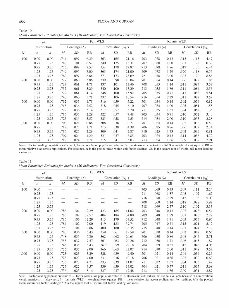
Table 10Mean Parameter Estimates for Model 3 (10 Indicators, Two Correlated Constructs)

N

y*distribution

Full WLS Robust WLS

Loadings (�) Correlation (�21) Loadings (�) Correlation (�21)


100 0.00 0.00 .744 .097 6.29 .363 .165 21.16 .703 .078 0.43 .313 .115 4.490.75 1.75 .746 .101 6.57 .340 .175 13.31 .707 .080 1.00 .301 .122 0.390.75 3.75 .753 .099 7.57 .354 .178 17.87 .713 .078 1.86 .319 .130 6.441.25 1.75 .749 .095 7.00 .363 .174 21.00 .709 .078 1.29 .320 .118 6.551.25 3.75 .762 .097 8.86 .371 .173 23.69 .721 .078 3.00 .327 .120 8.86

200 0.00 0.00 .727 .060 3.86 .339 .098 13.04 .701 .054 0.14 .306 .079 1.860.75 1.75 .733 .061 4.71 .337 .101 12.46 .708 .055 1.14 .311 .087 3.530.75 3.75 .737 .061 5.29 .340 .100 13.29 .713 .055 1.86 .311 .084 3.561.25 1.75 .729 .061 4.14 .348 .100 15.92 .705 .055 0.71 .317 .083 5.811.25 3.75 .740 .060 5.71 .332 .106 10.54 .716 .054 2.29 .311 .087 3.57

500 0.00 0.00 .712 .035 1.71 .316 .059 5.22 .701 .034 0.14 .302 .054 0.820.75 1.75 .718 .036 2.57 .318 .055 6.10 .707 .034 1.00 .305 .051 1.550.75 3.75 .722 .036 3.14 .317 .057 5.70 .711 .035 1.57 .304 .052 1.351.25 1.75 .716 .035 2.29 .322 .057 7.48 .705 .034 0.71 .310 .052 3.401.25 3.75 .725 .036 3.57 .323 .058 7.53 .714 .034 2.00 .310 .053 3.28

1,000 0.00 0.00 .706 .024 0.86 .308 .038 2.71 .701 .024 0.14 .302 .036 0.520.75 1.75 .712 .025 1.71 .313 .038 4.39 .706 .025 0.86 .306 .037 2.140.75 3.75 .716 .025 2.29 .309 .041 2.87 .710 .025 1.43 .302 .039 0.811.25 1.75 .709 .024 1.29 .321 .037 6.85 .703 .024 0.43 .314 .036 4.721.25 3.75 .719 .024 2.71 .315 .041 5.03 .713 .024 1.86 .309 .039 2.91

Note. Factor loading population value � .7; factor correlation population value � .3. s � skewness; k � kurtosis; WLS � weighted least squares; RB �mean relative bias across replications. For loadings, M is the pooled mean within-cell factor loadings; SD is the square root of within-cell factor loadingvariances.

Table 11Mean Parameter Estimates for Model 4 (20 Indicators, Two Correlated Constructs)

N

y*distribution

Full WLS Robust WLS

Loadings (�) Correlation (�21) Loadings (�) Correlation (�21)


100 0.00 — — — — — — — .703 .069 0.43 .307 .111 2.240.75 1.75 — — — — — — .711 .068 1.57 .305 .107 1.620.75 3.75 — — — — — — .716 .070 2.29 .315 .106 5.091.25 1.75 — — — — — — .708 .068 1.14 .318 .098 5.921.25 3.75 — — — — — — .718 .069 2.57 .310 .102 3.33

200 0.00 0.00 .786 .104 12.29 .423 .185 41.02 .703 .048 0.43 .302 .078 0.540.75 1.75 .788 .102 12.57 .404 .184 34.80 .709 .048 1.29 .307 .076 2.220.75 3.75 .786 .106 12.29 .413 .179 37.52 .712 .048 1.71 .303 .075 0.961.25 1.75 .784 .102 12.00 .419 .183 39.74 .705 .047 0.71 .315 .071 5.121.25 3.75 .790 .104 12.86 .400 .180 33.35 .715 .048 2.14 .307 .074 2.19

500 0.00 0.00 .745 .036 6.43 .359 .061 19.59 .701 .030 0.14 .302 .047 0.660.75 1.75 .748 .036 6.86 .362 .062 20.61 .706 .030 0.86 .308 .045 2.710.75 3.75 .753 .037 7.57 .361 .063 20.26 .712 .030 1.71 .306 .045 1.871.25 1.75 .745 .035 6.43 .367 .059 22.18 .704 .029 0.57 .312 .046 4.061.25 3.75 .756 .035 8.00 .366 .063 22.07 .714 .030 2.00 .311 .048 3.57

1,000 0.00 0.00 .723 .023 3.29 .328 .039 9.40 .701 .021 0.14 .301 .034 0.260.75 1.75 .728 .023 4.00 .331 .036 10.18 .706 .021 0.86 .302 .030 0.630.75 3.75 .733 .023 4.71 .333 .039 11.07 .711 .022 1.57 .304 .033 1.471.25 1.75 .725 .022 3.57 .339 .039 13.02 .704 .021 0.57 .311 .035 3.681.25 3.75 .736 .023 5.14 .337 .037 12.48 .713 .021 1.86 .309 .031 2.87

Note. Factor loading population value � .7, factor correlation population value � .3. Dashes indicate values that are not available because of noninvertibleweight matrices. s � skewness; k � kurtosis; WLS � weighted least squares; RB � mean relative bias across replications. For loadings, M is the pooledmean within-cell factor loadings; SD is the square root of within-cell factor loading variances.


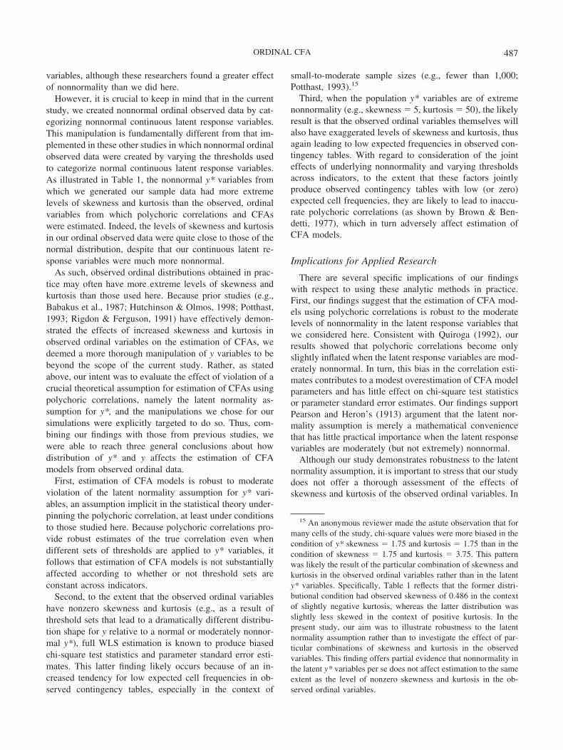
variables, although these researchers found a greater effectof nonnormality than we did here.

However, it is crucial to keep in mind that in the currentstudy, we created nonnormal ordinal observed data by cat-egorizing nonnormal continuous latent response variables.This manipulation is fundamentally different from that im-plemented in these other studies in which nonnormal ordinalobserved data were created by varying the thresholds usedto categorize normal continuous latent response variables.As illustrated in Table 1, the nonnormal y* variables fromwhich we generated our sample data had more extremelevels of skewness and kurtosis than the observed, ordinalvariables from which polychoric correlations and CFAswere estimated. Indeed, the levels of skewness and kurtosisin our ordinal observed data were quite close to those of thenormal distribution, despite that our continuous latent re-sponse variables were much more nonnormal.

As such, observed ordinal distributions obtained in prac-tice may often have more extreme levels of skewness andkurtosis than those used here. Because prior studies (e.g.,Babakus et al., 1987; Hutchinson & Olmos, 1998; Potthast,1993; Rigdon & Ferguson, 1991) have effectively demon-strated the effects of increased skewness and kurtosis inobserved ordinal variables on the estimation of CFAs, wedeemed a more thorough manipulation of y variables to bebeyond the scope of the current study. Rather, as statedabove, our intent was to evaluate the effect of violation of acrucial theoretical assumption for estimation of CFAs usingpolychoric correlations, namely the latent normality as-sumption for y*, and the manipulations we chose for oursimulations were explicitly targeted to do so. Thus, com-bining our findings with those from previous studies, wewere able to reach three general conclusions about howdistribution of y* and y affects the estimation of CFAmodels from observed ordinal data.

First, estimation of CFA models is robust to moderateviolation of the latent normality assumption for y* vari-ables, an assumption implicit in the statistical theory under-pinning the polychoric correlation, at least under conditionsto those studied here. Because polychoric correlations pro-vide robust estimates of the true correlation even whendifferent sets of thresholds are applied to y* variables, itfollows that estimation of CFA models is not substantiallyaffected according to whether or not threshold sets areconstant across indicators.

Second, to the extent that the observed ordinal variableshave nonzero skewness and kurtosis (e.g., as a result ofthreshold sets that lead to a dramatically different distribu-tion shape for y relative to a normal or moderately nonnor-mal y*), full WLS estimation is known to produce biasedchi-square test statistics and parameter standard error esti-mates. This latter finding likely occurs because of an in-creased tendency for low expected cell frequencies in ob-served contingency tables, especially in the context of

small-to-moderate sample sizes (e.g., fewer than 1,000;Potthast, 1993).15

Third, when the population y* variables are of extremenonnormality (e.g., skewness � 5, kurtosis � 50), the likelyresult is that the observed ordinal variables themselves willalso have exaggerated levels of skewness and kurtosis, thusagain leading to low expected frequencies in observed con-tingency tables. With regard to consideration of the jointeffects of underlying nonnormality and varying thresholdsacross indicators, to the extent that these factors jointlyproduce observed contingency tables with low (or zero)expected cell frequencies, they are likely to lead to inaccu-rate polychoric correlations (as shown by Brown & Ben-detti, 1977), which in turn adversely affect estimation ofCFA models.

Implications for Applied Research

There are several specific implications of our findingswith respect to using these analytic methods in practice.First, our findings suggest that the estimation of CFA mod-els using polychoric correlations is robust to the moderatelevels of nonnormality in the latent response variables thatwe considered here. Consistent with Quiroga (1992), ourresults showed that polychoric correlations become onlyslightly inflated when the latent response variables are mod-erately nonnormal. In turn, this bias in the correlation esti-mates contributes to a modest overestimation of CFA modelparameters and has little effect on chi-square test statisticsor parameter standard error estimates. Our findings supportPearson and Heron’s (1913) argument that the latent nor-mality assumption is merely a mathematical conveniencethat has little practical importance when the latent responsevariables are moderately (but not extremely) nonnormal.

Although our study demonstrates robustness to the latentnormality assumption, it is important to stress that our studydoes not offer a thorough assessment of the effects ofskewness and kurtosis of the observed ordinal variables. In

15 An anonymous reviewer made the astute observation that formany cells of the study, chi-square values were more biased in thecondition of y* skewness � 1.75 and kurtosis � 1.75 than in thecondition of skewness � 1.75 and kurtosis � 3.75. This patternwas likely the result of the particular combination of skewness andkurtosis in the observed ordinal variables rather than in the latenty* variables. Specifically, Table 1 reflects that the former distri-butional condition had observed skewness of 0.486 in the contextof slightly negative kurtosis, whereas the latter distribution wasslightly less skewed in the context of positive kurtosis. In thepresent study, our aim was to illustrate robustness to the latentnormality assumption rather than to investigate the effect of par-ticular combinations of skewness and kurtosis in the observedvariables. This finding offers partial evidence that nonnormality inthe latent y* variables per se does not affect estimation to the sameextent as the level of nonzero skewness and kurtosis in the ob-served ordinal variables.

487ORDINAL CFA

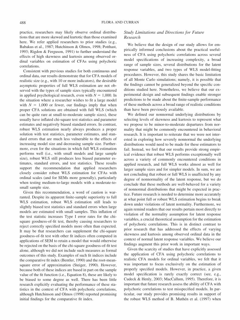
practice, researchers may likely observe ordinal distribu-tions that are more skewed and kurtotic than those examinedhere. We refer applied researchers to prior studies (e.g.,Babakus et al., 1987; Hutchinson & Olmos, 1998; Potthast,1993; Rigdon & Ferguson, 1991) to further understand theeffects of high skewness and kurtosis among observed or-dinal variables on estimation of CFAs using polychoriccorrelations.

Consistent with previous studies for both continuous andordinal data, our results demonstrate that for CFA models ofrealistic size (e.g., with 10 or more indicators), the desirableasymptotic properties of full WLS estimation are not ob-served with the types of sample sizes typically encounteredin applied psychological research, even with N � 1,000. Inthe situation where a researcher wishes to fit a large modelwith N � 1,000 or fewer, our findings imply that whenproper CFA solutions are obtained with full WLS (whichcan be quite rare at small-to-moderate sample sizes), theseusually have inflated chi-square test statistics and parameterestimates and negatively biased standard errors. In contrast,robust WLS estimation nearly always produces a propersolution with test statistics, parameter estimates, and stan-dard errors that are much less vulnerable to the effects ofincreasing model size and decreasing sample size. Further-more, even for the situations in which full WLS estimationperforms well (i.e., with small models and large samplesize), robust WLS still produces less biased parameter es-timates, standard errors, and test statistics. These resultssupport the recommendation that applied researchersclosely consider robust WLS estimation for CFAs withordinal scales (and for SEMs more generally), particularlywhen testing medium-to-large models with a moderate-to-small sample size.

Given this recommendation, a word of caution is war-ranted. Despite its apparent finite-sample superiority to fullWLS estimation, robust WLS estimation still leads toslightly biased test statistics and standard errors when largemodels are estimated with small samples. This inflation ofthe test statistic increases Type I error rates for the chi-square goodness-of-fit test, thereby causing researchers toreject correctly specified models more often than expected.It may be that researchers can supplement the chi-squaregoodness-of-fit test with other fit indices often computed inapplications of SEM to retain a model that would otherwisebe rejected on the basis of the chi-square goodness-of-fit testalone, although we did not include such measures as formaloutcomes of this study. Examples of such fit indices includethe comparative fit index (Bentler, 1990) and the root-mean-square error of approximation (Steiger, 1990). However,because both of these indices are based in part on the samplevalue of the fit function (i.e., Equation 8), these are likely tobe biased to some degree as well. There has been littleresearch explicitly evaluating the performance of these sta-tistics in the context of CFA with polychoric correlations,although Hutchinson and Olmos (1998) reported promisinginitial findings for the comparative fit index.

Study Limitations and Directions for FutureResearch

We believe that the design of our study allows for em-pirically informed conclusions about the practical useful-ness of CFA using polychoric correlations across severalmodel specifications of increasing complexity, a broadrange of sample sizes, several distributions for the latentresponse variables, and two types of WLS model-fittingprocedures. However, this study shares the basic limitationof all Monte Carlo simulations; namely, it is possible thatthe findings cannot be generalized beyond the specific con-ditions studied here. Nonetheless, we believe that our ex-perimental design and subsequent findings enable strongerpredictions to be made about the finite-sample performanceof these methods across a broad range of realistic conditionsthan have been previously available.

We defined our nonnormal underlying distributions byselecting levels of skewness and kurtosis to represent whatwe propose to be minor-to-moderate departures from nor-mality that might be commonly encountered in behavioralresearch. It is important to reiterate that we were not inter-ested in exploring how severely nonnormal the underlyingdistributions would need to be made for these estimators tofail. Instead, we feel that our results provide strong empir-ical evidence that robust WLS performs exceptionally wellacross a variety of commonly encountered conditions inapplied research, and full WLS works almost as well forlarger sample sizes and for simpler models. In sum, we arenot concluding that robust or full WLS is unaffected by anydegree of nonnormality of the latent response, but we doconclude that these methods are well-behaved for a varietyof nonnormal distributions that might be expected in prac-tice. Future research is needed to determine more accuratelyat what point full or robust WLS estimation begins to breakdown under violations of latent normality. Furthermore, weagain remind readers that our results pertain most directly toviolation of the normality assumption for latent responsevariables, a crucial theoretical assumption for the estimationof polychoric correlations. This is in distinct contrast toprior research that has addressed the effects of varyingskewness and kurtosis among observed ordinal data in thecontext of normal latent response variables. We believe ourfindings augment this prior work in important ways.

Given the scarcity of studies that have explicitly assessedthe application of CFA using polychoric correlations torealistic CFA models for ordinal variables, we felt that itwas important to focus exclusively on the estimation ofproperly specified models. However, in practice, a givenmodel specification is rarely exactly correct (see, e.g.,Cudeck & Henly, 2003; MacCallum, 1995). Therefore, it isimportant that future research assess the ability of CFA withpolychoric correlations to test misspecified models. In par-ticular, our study provides promising results in support ofthe robust WLS method of B. Muthen et al. (1997) when


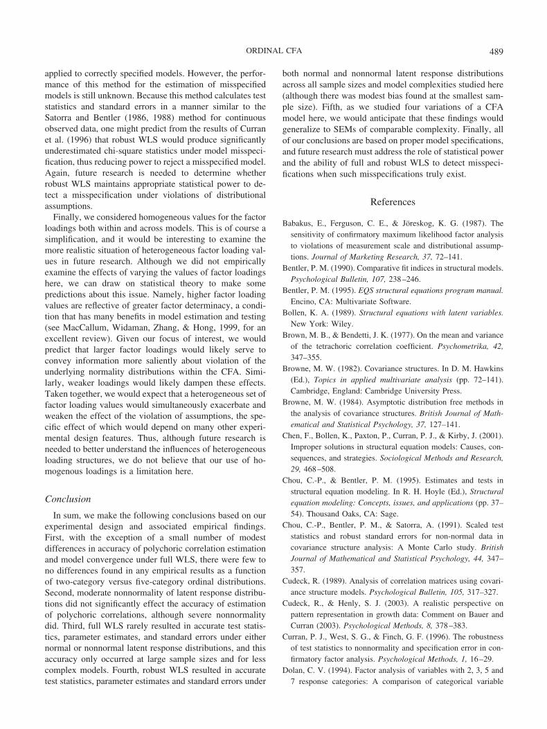
applied to correctly specified models. However, the perfor-mance of this method for the estimation of misspecifiedmodels is still unknown. Because this method calculates teststatistics and standard errors in a manner similar to theSatorra and Bentler (1986, 1988) method for continuousobserved data, one might predict from the results of Curranet al. (1996) that robust WLS would produce significantlyunderestimated chi-square statistics under model misspeci-fication, thus reducing power to reject a misspecified model.Again, future research is needed to determine whetherrobust WLS maintains appropriate statistical power to de-tect a misspecification under violations of distributionalassumptions.

Finally, we considered homogeneous values for the factorloadings both within and across models. This is of course asimplification, and it would be interesting to examine themore realistic situation of heterogeneous factor loading val-ues in future research. Although we did not empiricallyexamine the effects of varying the values of factor loadingshere, we can draw on statistical theory to make somepredictions about this issue. Namely, higher factor loadingvalues are reflective of greater factor determinacy, a condi-tion that has many benefits in model estimation and testing(see MacCallum, Widaman, Zhang, & Hong, 1999, for anexcellent review). Given our focus of interest, we wouldpredict that larger factor loadings would likely serve toconvey information more saliently about violation of theunderlying normality distributions within the CFA. Simi-larly, weaker loadings would likely dampen these effects.Taken together, we would expect that a heterogeneous set offactor loading values would simultaneously exacerbate andweaken the effect of the violation of assumptions, the spe-cific effect of which would depend on many other experi-mental design features. Thus, although future research isneeded to better understand the influences of heterogeneousloading structures, we do not believe that our use of ho-mogenous loadings is a limitation here.

Conclusion

In sum, we make the following conclusions based on ourexperimental design and associated empirical findings.First, with the exception of a small number of modestdifferences in accuracy of polychoric correlation estimationand model convergence under full WLS, there were few tono differences found in any empirical results as a functionof two-category versus five-category ordinal distributions.Second, moderate nonnormality of latent response distribu-tions did not significantly effect the accuracy of estimationof polychoric correlations, although severe nonnormalitydid. Third, full WLS rarely resulted in accurate test statis-tics, parameter estimates, and standard errors under eithernormal or nonnormal latent response distributions, and thisaccuracy only occurred at large sample sizes and for lesscomplex models. Fourth, robust WLS resulted in accuratetest statistics, parameter estimates and standard errors under

both normal and nonnormal latent response distributionsacross all sample sizes and model complexities studied here(although there was modest bias found at the smallest sam-ple size). Fifth, as we studied four variations of a CFAmodel here, we would anticipate that these findings wouldgeneralize to SEMs of comparable complexity. Finally, allof our conclusions are based on proper model specifications,and future research must address the role of statistical powerand the ability of full and robust WLS to detect misspeci-fications when such misspecifications truly exist.

References

Babakus, E., Ferguson, C. E., & Joreskog, K. G. (1987). Thesensitivity of confirmatory maximum likelihood factor analysisto violations of measurement scale and distributional assump-tions. Journal of Marketing Research, 37, 72–141.

Bentler, P. M. (1990). Comparative fit indices in structural models.Psychological Bulletin, 107, 238–246.

Bentler, P. M. (1995). EQS structural equations program manual.Encino, CA: Multivariate Software.

Bollen, K. A. (1989). Structural equations with latent variables.New York: Wiley.

Brown, M. B., & Bendetti, J. K. (1977). On the mean and varianceof the tetrachoric correlation coefficient. Psychometrika, 42,347–355.

Browne, M. W. (1982). Covariance structures. In D. M. Hawkins(Ed.), Topics in applied multivariate analysis (pp. 72–141).Cambridge, England: Cambridge University Press.

Browne, M. W. (1984). Asymptotic distribution free methods inthe analysis of covariance structures. British Journal of Math-ematical and Statistical Psychology, 37, 127–141.

Chen, F., Bollen, K., Paxton, P., Curran, P. J., & Kirby, J. (2001).Improper solutions in structural equation models: Causes, con-sequences, and strategies. Sociological Methods and Research,29, 468–508.

Chou, C.-P., & Bentler, P. M. (1995). Estimates and tests instructural equation modeling. In R. H. Hoyle (Ed.), Structuralequation modeling: Concepts, issues, and applications (pp. 37–54). Thousand Oaks, CA: Sage.

Chou, C.-P., Bentler, P. M., & Satorra, A. (1991). Scaled teststatistics and robust standard errors for non-normal data incovariance structure analysis: A Monte Carlo study. BritishJournal of Mathematical and Statistical Psychology, 44, 347–357.

Cudeck, R. (1989). Analysis of correlation matrices using covari-ance structure models. Psychological Bulletin, 105, 317–327.

Cudeck, R., & Henly, S. J. (2003). A realistic perspective onpattern representation in growth data: Comment on Bauer andCurran (2003). Psychological Methods, 8, 378–383.

Curran, P. J., West, S. G., & Finch, G. F. (1996). The robustnessof test statistics to nonnormality and specification error in con-firmatory factor analysis. Psychological Methods, 1, 16–29.

Dolan, C. V. (1994). Factor analysis of variables with 2, 3, 5 and7 response categories: A comparison of categorical variable

489ORDINAL CFA

estimators using simulated data. British Journal of Mathemati-cal and Statistical Psychology, 47, 309–326.

Fleishman, A. I. (1978). A method for simulating non-normaldistributions. Psychometrika, 43, 521–532.

Green, S. B., Akey, T. M., Fleming, K. K., Hershberger, S. L., &Marquis, J. G. (1997). Effect of the number of scale points onchi-square fit indices in confirmatory factor analysis. StructuralEquation Modeling, 4, 108–120.

Hu, L.-T., Bentler, P. M., & Kano, Y. (1992). Can test statistics incovariance structure analysis be trusted? Psychological Bulletin,112, 351–362.

Hutchinson, S. R., & Olmos, A. (1998). Behavior of descriptive fitindexes in confirmatory factor analysis using ordered categori-cal data. Structural Equation Modeling, 5, 344–364.

Joreskog, K. G. (1969). A general approach to confirmatory max-imum likelihood factor analysis. Psychometrika, 34, 183–202.

Joreskog, K. G. (1994). On the estimation of polychoric correla-tions and their asymptotic covariance matrix. Psychometrika,59, 381–389.

Joreskog, K. G., & Sorbom, D. (1988). PRELIS: A program formultivariate data screening and data summarization. A pre-processor for LISREL (2nd ed.). Mooresville, IN: ScientificSoftware.

Joreskog, K. G., & Sorbom, D. (1996). LISREL 8: User’s refer-ence guide. Chicago: Scientific Software.

Kaplan, D. (1989). A study of the sampling variability of thez-values of parameter estimates from misspecified structuralequation models. Multivariate Behavioral Research, 24, 41–57.

Lord, F. M., & Novick, M. R. (1968). Statistical theories of mentaltest scores. Reading, MA: Addison-Wesley.

MacCallum, R. C. (1995). Model specification: Procedures, strat-egies, and related issues. In R. Hoyle (Ed.), Structural equationmodeling: Concepts, issues, and applications (pp. 16–36).Thousand Oaks, CA: Sage.

MacCallum, R. C., Widaman, K. F., Zhang, S., & Hong, S. (1999).Sample size in factor analysis. Psychological Methods, 4, 84–99.

Micceri, T. (1989). The unicorn, the normal curve, and otherimprobable creatures. Psychological Bulletin, 105, 156–166.

Muthen, B. (1983). Latent variable structural equation modelingwith categorical data. Journal of Econometrics, 22, 48–65.

Muthen, B. (1984). A general structural equation model withdichotomous, ordered categorical, and continuous latent vari-able indicators. Psychometrika, 49, 115–132.

Muthen, B., du Toit, S. H. C., & Spisic, D. (1997). Robustinference using weighted least squares and quadratic estimatingequations in latent variable modeling with categorical andcontinuous outcomes. Unpublished manuscript.

Muthen, B., & Hofacker, C. (1988). Testing the assumptionsunderlying tetrachoric correlations. Psychometrika, 53, 563–578.

Muthen, B., & Kaplan, D. (1985). A comparison of some meth-odologies for the factor-analysis of non-normal Likert variables.British Journal of Mathematical and Statistical Psychology, 38,171–180.

Muthen, B., & Kaplan, D. (1992). A comparison of some meth-odologies for the factor-analysis of non-normal Likert variables:A note on the size of the model. British Journal of Mathematical

and Statistical Psychology, 45, 19–30.Muthen, B. O., & Satorra, A. (1995). Technical aspects of Muth-

en’s LISCOMP approach to estimation of latent variable rela-tions with a comprehensive measurement model. Psy-

chometrika, 60, 489–503.Muthen, L. K., & Muthen, B. O. (1998). Mplus user’s guide. Los

Angeles: Author.Neale, M. C., Boker, S. M., Xie, G., & Maes, H. H. (2002). Mx:

Statistical modeling (6th ed.). Richmond, VA: Department ofPsychiatry, Virginia Commonwealth University.

Olsson, U. (1979). Maximum likelihood estimation of the poly-choric correlation coefficient. Psychometrika, 44, 443–460.

Pearson, K. (1901). Mathematical contributions to the theory ofevolution, VII: On the correlation of characters not quantita-tively measurable. Philosophical Transactions of the Royal So-

ciety of London, Series A, 195, 1–47.Pearson, K., & Heron, D. (1913). On theories of association.

Biometrika, 9, 159–315.Potthast, M. J. (1993). Confirmatory factor analysis of ordered

categorical variables with large models. British Journal of

Mathematical and Statistical Psychology, 46, 273–286.Quiroga, A. M. (1992). Studies of the polychoric correlation and

other correlation measures for ordinal variables. Unpublisheddoctoral dissertation, Acta Universitatis Upsaliensis.

Rigdon, E. E., & Ferguson, C. E. (1991). The performance of thepolychoric correlation coefficient and selected fitting functionsin confirmatory factor analysis with ordinal data. Journal of

Marketing Research, 28, 491–497.Satorra, A. (1992). Asymptotic robust inferences in the analysis of

mean and covariance structures. In P. Marsden (Ed.), Sociolog-

ical methodology 1992. Washington, DC: American Sociologi-cal Association.

Satorra, A., & Bentler, P. M. (1986). Some robustness propertiesof goodness of fit statistics in covariance structure analysis.1986 ASA Proceedings of the Business and Economic Section,

549–554.Satorra, A., & Bentler, P. M. (1988). Scaling corrections for

chi-square statistics in covariance structure analysis. 1988 ASA

Proceedings of the Business and Economic Section, 308–313.Satorra, A., & Bentler, P. M. (1990). Model conditions for asymp-

totic robustness in the analysis of linear relations. Computa-

tional Statistics and Data Analysis, 10, 235–249.Satterthwaite, F. E. (1941). Synthesis of variance. Psychometrika,

6, 309–316.Shadish, W. R., Cook, T. D., & Campbell, D. T. (2002). Experi-

mental and quasi-experimental designs for generalized causal

inference. Boston: Houghton-Mifflin.Steiger, J. H. (1990). Structural model evaluation and modifica-

tion: An interval estimation approach. Multivariate Behavioral

Research, 25, 173–180.


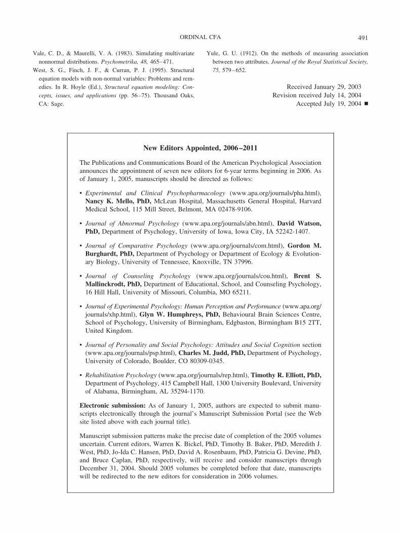
Vale, C. D., & Maurelli, V. A. (1983). Simulating multivariatenonnormal distributions. Psychometrika, 48, 465–471.

West, S. G., Finch, J. F., & Curran, P. J. (1995). Structuralequation models with non-normal variables: Problems and rem-edies. In R. Hoyle (Ed.), Structural equation modeling: Con-

cepts, issues, and applications (pp. 56–75). Thousand Oaks,CA: Sage.

Yule, G. U. (1912). On the methods of measuring associationbetween two attributes. Journal of the Royal Statistical Society,

75, 579–652.

Received January 29, 2003Revision received July 14, 2004

Accepted July 19, 2004 �

New Editors Appointed, 2006–2011

The Publications and Communications Board of the American Psychological Associationannounces the appointment of seven new editors for 6-year terms beginning in 2006. Asof January 1, 2005, manuscripts should be directed as follows:

• Experimental and Clinical Psychopharmacology (www.apa.org/journals/pha.html),Nancy K. Mello, PhD, McLean Hospital, Massachusetts General Hospital, HarvardMedical School, 115 Mill Street, Belmont, MA 02478-9106.

• Journal of Abnormal Psychology (www.apa.org/journals/abn.html), David Watson,PhD, Department of Psychology, University of Iowa, Iowa City, IA 52242-1407.

• Journal of Comparative Psychology (www.apa.org/journals/com.html), Gordon M.Burghardt, PhD, Department of Psychology or Department of Ecology & Evolution-ary Biology, University of Tennessee, Knoxville, TN 37996.

• Journal of Counseling Psychology (www.apa.org/journals/cou.html), Brent S.Mallinckrodt, PhD, Department of Educational, School, and Counseling Psychology,16 Hill Hall, University of Missouri, Columbia, MO 65211.

• Journal of Experimental Psychology: Human Perception and Performance (www.apa.org/journals/xhp.html), Glyn W. Humphreys, PhD, Behavioural Brain Sciences Centre,School of Psychology, University of Birmingham, Edgbaston, Birmingham B15 2TT,United Kingdom.

• Journal of Personality and Social Psychology: Attitudes and Social Cognition section(www.apa.org/journals/psp.html), Charles M. Judd, PhD, Department of Psychology,University of Colorado, Boulder, CO 80309-0345.

• Rehabilitation Psychology (www.apa.org/journals/rep.html), Timothy R. Elliott, PhD,Department of Psychology, 415 Campbell Hall, 1300 University Boulevard, Universityof Alabama, Birmingham, AL 35294-1170.

Electronic submission: As of January 1, 2005, authors are expected to submit manu-scripts electronically through the journal’s Manuscript Submission Portal (see the Website listed above with each journal title).

Manuscript submission patterns make the precise date of completion of the 2005 volumesuncertain. Current editors, Warren K. Bickel, PhD, Timothy B. Baker, PhD, Meredith J.West, PhD, Jo-Ida C. Hansen, PhD, David A. Rosenbaum, PhD, Patricia G. Devine, PhD,and Bruce Caplan, PhD, respectively, will receive and consider manuscripts throughDecember 31, 2004. Should 2005 volumes be completed before that date, manuscriptswill be redirected to the new editors for consideration in 2006 volumes.

491ORDINAL CFA

an empirical evaluation of alternative methods of ...an empirical evaluation of alternative methods...

Documents