Journal of Mathematical Finance, 2017, 7, 366-390 http://www.scirp.org/journal/jmf

ISSN Online: 2162-2442 ISSN Print: 2162-2434

DOI: 10.4236/jmf.2017.72020 May 19, 2017

An Empirical Evaluation in GARCH Volatility Modeling: Evidence from the Stockholm Stock Exchange

Chaido Dritsaki

Department of Accounting and Finance, Western Macedonia University of Applied Sciences, Kozani, Greece

Abstract In this paper, we use daily stock returns from the Stockholm Stock Exchange in order to examine their volatility. For this reason, we estimate not only GARCH (1,1) symmetric model but also asymmetric models EGARCH (1,1) and GJR-GARCH (1,1) with different residual distributions. The parameters of the volatility models are estimated with the Maximum Likelihood (ML) using the Marquardt algorithm (Marquardt [1]). The findings reveal that neg-ative shocks have a large impact than positive shocks in this market. Also, in-dices for the return of forecasting have shown that the ARIMA (0,0,1)- EGARCH (1,1) model with t-student provide more precise forecasting on vo-latilities and expected returns of the Stockholm Stock Exchange.

Keywords Stockholm Stock Exchange, Volatility, GARCH Models, Leverage Effect, Forecasting

1. Introduction

The development of econometrics led to the invention of adjusted methodolo-gies for the modeling of mean value and variance. Models of generalized condi-tional autoregressive heteroscedasticity (GARCH) are based on the assumption that random components in models present changes on volatility. These models were developed by Engle [2], in a simple form, and they were generalized later by Bollerslev [3].

The models of autoregressive conditional heteroscedasticity (GARCH) have a long and noteworthy history but they are not free of limitations. For example, Black [4] on his paper claims that stock market returns are negatively correlated with changes on volatility returns implying that volatility tends to rise in re-

How to cite this paper: Dritsaki, C. (2017) An Empirical Evaluation in GARCH Vola-tility Modeling: Evidence from the Stock-holm Stock Exchange. Journal of Mathe-matical Finance, 7, 366-390. https://doi.org/10.4236/jmf.2017.72020 Received: March 4, 2017 Accepted: May 15, 2017 Published: May 19, 2017 Copyright © 2017 by author and Scientific Research Publishing Inc. This work is licensed under the Creative Commons Attribution International License (CC BY 4.0). http://creativecommons.org/licenses/by/4.0/

Open Access

C. Dritsaki

367

sponse to bad news and fall in response to good news. On the other hand, on GARCH models we assume that only the size of return of the conditional variance is defined and not the positivity or negativity of volatility’s return, which are unpredicted. Another crucial limitation of GARCH models is the non-negativity of parameters in order to ensure the positivity of the conditional variance. All these limitations cause difficulties in the estimation of GARCH models.

GARCH models were applied with great success on the modeling of changing variability or the variance volatility on time series for measuring financial in-vestments. After the determination of an asymmetric relationship between con-ditional volatility and conditional mean value, econometricians focused their ef-forts on planning methodologies for modeling this phenomenon.

Nelson [5] suggested an exponential GARCH model (EGARCH) expressed in logarithms of the conditional variance volatility. The EGARCH model has be-come popular as it presents asymmetric volatility on positive and negative re-turns. A number of modifications on this model were made over the years. Glosten, Jagannathan and Runkle [6] suggest another asymmetric model known as GJR-GARCH which deals with the limitations of the symmetric GARCH models.

The purpose of this paper is to quantify two asymmetric models using prices from the Stockholm stock market for the period 30 September 1986 until 11 May 2016, representing 7,434 observations. The first 7,000 values in the model were used for quantification and statistical verification and the last 434 values for the forecast demonstration in retrospect.

The remainder of the paper is organized as follows: Section 2 provides a brief literature review. Section 3 discusses the symmetric and asymmetric GARCH models. Section 4 summarizes the data. The results are discussed in Section 5 and Section 6 proposes the forecasting methodology. Finally, the last section of-fers the concluding remarks.

2. Literature Review

The ability of GARCH models that study the relationship between risk and re-turn has been validated in many studies. For example, Donaldson and Kamstra [7] made a nonlinear GARCH model based on neural networks. They evaluated the model’s ability in forecasting the volatility of returns on the stock markets of London, New York, Tokyo and Toronto. The results of their paper showed that neural network models captures volatility effects and forecasting better than GARCH, EGARCH and GJR models.

Nam, Pyun and Arize [8] used the asymmetric non-linear GARCH-M model for US market indices for the period 1926:01-1997:12. The results of their paper showed that negative returns on average reverted more quickly in the long term rather than positive returns.

Tudor [9] uses GARCH and GARCH-M models to examine the volatility of US and Romanian stock markets for the period January, 03 2001 until February 09, 2008 or a total of 1,853 daily returns. The results showed that the GARCH-M

C. Dritsaki

368

model performs better and confirms the results between volatility and expected returns on both markets.

Panait and Slavescu [10] use daily, weekly and monthly data for seven Roma-nian listed companies on the Bucharest stock market for the period 1997-2012. Using the GARCH-in-mean model they compare the volatility of companies in three phases. The results of their paper showed that persistency is more evident in the daily returns rather than in the weekly and monthly series. Furthermore, the GARCH-in-mean model failed to confirm that an increase in volatility leads to a rise in future returns.

Gao, Zhang and Zhang [11] use the Markov chain Monte Carlo (MCMC) method instead of the Maximum Likelihood Ratio method for the estimation of the coefficients of GARCH models. Using daily data from the stock market of China for the period 1 January 2000 until 29 April 2011, they compare the re-sults of the volatility of the data with three different models and two different distributions. The results showed that the GED-GARCH model is better than the t-GARCH, and that the t-GARCH is better than N-GARCH.

Dutta [12] examined exchange rate parities of USA and Japan for the period 1 January 2000 until 31 January 2012. The data are estimated not only with sym-metric but also with asymmetric GARCH models. Findings indicate that positive shocks are more common than the negative shocks in this return series. Also, asymmetric tests for volatility show a size effect on news, which is stronger for good news than for bad news.

Given the different backgrounds for each market it is expected that risk and return differ from country to country. This paper attempts to examine the vola-tility and return of the Stockholm stock market using symmetric and asymme-tric models.

3. Methodology

One of the fundamental hypotheses for a stationary time series is the stable va-riance. But there are time series, mostly financial, that have intervals of large vo-latility. These series are characterized with periods of sharp increases and downturns during which their variance is varying. Thus, researchers are not in-terested in examining the variance of such series throughout the sample period but only interested in the varying or conditional variance. Based on this division between conditional and unconditional variance, we can characterize time series models with conditional variance as conditional heteroskedastic models. The notion of “conditional” heteroscedasticity was first introduced by Engle [2]. En-gle suggested that varying variance can be explained through an autoregressive scheme as a function of previous values. For this reason this model is called Au-toregressive Conditional Heteroskedastic Model, known as ARCH.

The varying GARCH models consist of two equations. The first one (the equ-ation of mean) describes the data as a function of other variables adding an error term. The second equation (the equation of variance) determines the evolution of the conditional variance of the error from the mean equation as a function of

C. Dritsaki

369

past conditional variances and lagged errors. The first equation (equation of the mean) on GARCH varying models is not of great interest, contrary to the second equation (equation of variance) which is the one that we pay more attention to in order to compare different variances on the same equation of mean.

3.1. Symmetric GARCH Models

The traditional measuring methods of volatility (variance or standard deviation) are absolute and cannot conceive the characteristics of financial data (time series) like volatility clustering, asymmetries, leverage effect and long memory. The ba-sic model suggested by Engel [2] is the following:

t t tzε σ=

where tz is an independent identically distributed (i.i.d.) process with mean zero and variance 1. tσ is the volatility that evolves over time. The volatility

2tσ in the basic ARCH (q) model is defined as:

2 2

1

q

t i t ii

σ ω α ε −=

= +∑ (1)

where 2tσ is the conditional variance, 0ω > and 0iα ≥ for 2

tσ to be posi-tive.

This model shows that after a large (small) shock, it is likely that a large (small) shock will follow. In other words, a large (small) 2

1tε − implies a large (small) 2tε on the current period according to Equation (1) thus a large (small) variance

(volatility). Finally, we can point out that large values on time lags on ARCH models pre-

suppose large periods of volatility contrary to small values of time lags that fore-see smooth periods. This may not occur in reality. In order to overcome this problem, Bollerslev, Chou and Kroner [13] suggested a new model where the conditional variance does not depend only on previous square error values but also on previous values of the same variance. The model suggested is known as Generalized Autoregressive Conditional Heteroskedasticity (GARCH) model.

GARCH (p, q) Model The generalized form of GARCH(p, q) is given as:

t tR µ ε= + (mean equation)

2 2 2

1 1

q p

t i t i j t ji j

σ ω α ε β σ− −= =

= + +∑ ∑ (variance equation) (2)

where tR are returns of time series at time t, µ is the mean value of the re-turns, tε is the error term at time t, which is assumed to be normally distri-buted with zero mean and conditional variance 2

tσ , p is the order of GARCH and q is the order of ARCH process, µ , ω , iα and jβ are parameters for estimation. All parameters in variance equation must be positive ( 0µ > , 0ω > ,

0iα ≥ , and 0jβ ≥ for 2tσ to be positive). Also, we expect the value of para-

meter ω to be small. Parameter iα measures the response of volatility on mar-

C. Dritsaki

370

ket variances and parameter jβ expresses the difference which was caused from outliers on conditional variance. Finally, we expect the sum 1i jα β+ <

The model GARCH (1,1) has the following form:

t tR µ ε= + (mean equation)

2 2 21 1 1 1t t tσ ω α ε β σ− −= + + (variance equation) (3)

As we expect a positive variance, we can argue that regression coefficients are always positive 0ω ≥ , 1 0α ≥ and 1 0β ≥ . Also, we should point out that in order to achieve stationarity on the variance, regression coefficients 1α and

1β should be less than one ( )1 1α < and ( )1 1β < . Thus, on the previous mod-el, the following relations are valid: 0ω ≥ 1 0α ≥ and 1 0β ≥ for a positive value of 2

tσ and 1 1α < and 1 1β < . The conditional variance of the returns of Equation (3) is defined from three

outcomes: • The constant given by ω coefficient. • The variance part expressed from the relationship 2

1 1tα ε − defined as ARCH component.

• The part of predicted variance from past period expressed by 21 1tβ σ − and is

called GARCH. The sum of regression coefficients 1 1α β+ expresses the impact of variables’

variance of the previous period regarding the current value of volatility. This value is usually near to one and is regarded as a sign of increasing inactivity of shocks of the volatility of returns on the financial assets.

3.2. Asymmetric GARCH Models

The main disadvantage of GARCH models is their inappropriateness in the cases where an asymmetric effect is usually observed and is registered from a different instability in the case of good and bad news. In the asymmetric models, upward and downward trends of returns are interpreted as bad and good news. If the de-cline of a return is accompanied with an increase of instability larger than the instability caused by the increase then it is said to have a leverage effect.

Given that all terms in a GARCH model are squared, there will always be an asymmetric response in positive and negative periods. However, due to natural leverage in most companies, a negative shock is more damaging than a positive shock because it produces larger volatility.

Among the most widely known asymmetric models are the Exponential GARCH model (EGARCH) and the asymmetric GJR model.

3.2.1. Asymmetric GARCH Models One of the most popular asymmetric ARCH models is the EGARCH model proposed by Nelson [5]. The EGARCH (p, q) model is given by

2 2

1 1 1log log

p q rt i t k

t i j t j ki j kt i t k

ε εσ ω α β σ γ

σ σ− −

−= = =− −

= + + +∑ ∑ ∑ (4)

where ω , iα , jβ , and kγ are parameters which can be estimated using the

C. Dritsaki

371

maximum likelihood method. We should also point out that 1jβ < and kγ parameter is the one that gives the result of leverage effect. In other words, we consider that t kε − term is the one that establishes the asymmetry of EGARCH (p, q) when parameter 0kγ ≠ . Also, when parameter 0kγ < , then positive shocks cause short volatility in relation to negative shocks. Furthermore, we ex-pect that parameters 0k iγ α+ > , given that parameter 0kγ < .

The conditional variance of the above model is expressed in logarithmic form which ensures the non-negativity without imposing more constraints of non-

negativity. The term t k

t k

εσ

−

−

on the above equation represents the asymmetric

effect of shocks. According to Poon and Granger [14], a negative shock that leads to the largest conditional variance will not be the same on a positive shock in the next period.

The EGARCH (1,1) model is often used for the estimation of variance 2σ and has the following form:

2 21 11 1 1 1

1 1

log logt tt t

t t

ε εσ ω α β σ γ

σ σ− −

−− −

= + + + (5)

For a positive shock 1

1

0t

t

εσ

−

−

> the above equation becomes

( )2 2 11 1 1 1

1

log log tt t

t

εσ ω β σ α γ

σ−

−−

= + + + (6)

whereas for a negative shock 1

1

0t

t

εσ

−

−

< the above equation becomes

( )2 2 11 1 1 1

1

log log tt t

t

εσ ω β σ α γ

σ−

−−

= + + − (7)

The EGARCH model has many advantages when compared to the GARCH (p, q) model. • The first is the logarithmic form which does not allow the positive constraint

among parameters. • Another advantage of EGARCH model is that it incorporates asymmetries in

the change of volatility of returns. • Parameters α and γ define two important asymmetries in the condition-

al variance. If 1 0γ < then negative changes increase volatility (instability) more than positive changes of the same size.

• EGARCH model can successfully define the change of volatility. The form of the EGARCH model denotes that the conditional variance is an

exponential function of the examined variables which ensures a positive charac-ter. In other words, conditional variance ensures the exponential nature of the EGARCH model where external changes will have a stronger influence on the predicted volatility than TGARCH. An asymmetric influence is indicated by the no null value of γ1 coefficient whereas the presence of leverage is indicated by the negative value of the same coefficient.

C. Dritsaki

372

3.2.2. The GJR-GARCH Model The GJR-GARCH(p, q) model is another asymmetric GARCH model proposed by Glosten, Jagannatahan and Runkle [6]. The generalized form of the GJR- GARCH (p, q) model is given in the following form:

2 2 2

1 1

p q

t i t i j t j i t i t ii j

Iδσ ω α ε β σ γ ε− − − −= =

= + + +∑ ∑ (8)

1 when 00 when 0

t it i

t i

Iεε

−−

−

<= ≥

when ω , iα , jβ and iγ are parameters under estimation

t iI − is a dummy variable, meaning that t iI − is a functional index which takes zero value when t iε − is positive and value one when t iε − is negative. If para-meter 0iγ > then negative errors are leveraged meaning that negative innova-tions or bad news have larger impact than good news. Finally, we assume that on the GJR-GARCH model parameters are positive and the relationship

12

ii j

γα β+ + < is valid.

The GJR-GARCH (1,1) model is the one that is more often used for the esti-mation of 2σ variance and has the following form:

2 2 2 21 1 1 1 1 1t t t t tIσ ω α ε β σ γ ε− − −= + + + (9)

11

1

1 when 00 when 0

tt

t

Iεε−

−−

<= ≥

Engle and Ng [15] compare the response of conditional variance to shocks implied by various econometric models and find evidence that the GJR model fits stock return data the best.

3.3. Estimation of the GARCH Model

The estimation of GARCH models can be done with the Ordinary Least Squares method. Due to the fact that error terms are not independently and identically distributed iid(0,1), it is better to avoid using the OLS method mainly on small samples. In this case, it is better to use the maximum likelihood method(see Greene, [16]). The parameters of GARCH models maximize the log likelihood function. The estimation of parameters on the log likelihood function derives through nonlinear least squares using Marquardt’s algorithm [1]. The log like-lihood function is given below:

( ) ( )( ) ( )2

1

1ln , ln , ln2

T

t t tt

L y D zθ θ υ σ θ=

= − ∑ (10)

where θ is the vector of the parameters that have to be estimated for the con-ditional mean, conditional variance and density function, tz denoting their density function, ( )( ),tD z θ υ , is the log-likelihood function of ( )ty θ , for a sample of T observation. The maximum likelihood estimator θ̂ for the true parameter vector is found by maximizing (10).

The models GARCH assumed Gaussian innovations, but nonetheless imply

C. Dritsaki

373

non-Gaussian unconditional distributions. However, time-varying volatility models with Gaussian innovations generally do not generate sufficient uncondi-tional non-Gaussianity to match certain financial asset return data (see, Poon and Granger [14]).

3.3.1. Conditional Distributions In this section we describe the log-likelihood functions used for the estimation of parameters on volatility models for all theoretical distributions.

1) Normal Distribution In the case of a standard normal distribution for the i.i.d. random variables

{ }tz , the following log-likelihood function needs to be maximized.

( ) ( ) ( )2 2

1 1

1ln , ln 2π ln2

T T

t t tt t

L y T zθ σ= =

= − + + ∑ ∑ (11)

where θ is the vector of the parameters that have to be estimated for the con-ditional mean, conditional variance and density function, T is observations.

2) Student-t Distribution The Student-t distribution can handle more severe leptokurtosis. The log-

likelihood function is defined as

( ) ( )

( ) ( )2

2

1

1 1ln , ln ln ln 22 2 2

1 ln 1 ln 12 2

t

Tt

tt

L y T

z

υ υθ π υ

σ υυ=

+ = Γ − Γ − −

− + + + −

∑ (12)

where ( ) 10

e dx x xυυ∞ − −Γ = ∫ is the gamma function and υ is the degree of

freedom. The t-Student is symmetric around zero. The Student-t distribution incorpo-

rates the standard normal distribution as a special case when υ = ∞ and the Cauchy distribution when 1υ = . Hence, a lower value, υ yields a distribution with “fatter tails”.

3.3.2. Generalized Error Distribution Nelson [5] proposed the use of GED when estimating EGARCH since it is more appealing in terms of fulfilling stationarity compared tο the Student-t distribu-tion. In the case of a t-Student distribution the unconditional means and va-riances may not be finite in the EGARCH. The log-likelihood function for the standard GED is defined as

( ) ( ) ( ) ( )1 2

1

1 1 1ln , ln 1 ln 2 ln ln2 2

Tt

t tt

zL y

υυθ υ σλ λ υ

−

=

= − − + − Γ − ∑ (13)

where

1 2

2

1

23

υ υλ

υ

−

Γ =

Γ

The distribution of generalized error (GED) incorporates both normal distri-bution when ( 2υ = ), Laplace distribution when ( 1υ = ), and the unique distri-

C. Dritsaki

374

bution for υ = ∞ . Specifically, we would say when 2υ = the distribution of the random variable zt would be the standard normal distribution. When 2υ < , the distribution of the random variable zt, will have thicker tails than that of normal distribution. For 1υ = the distribution of the random variable zt will have a double exponential distribution. For 2υ > the distribution of the ran-dom variable zt will have thinner tails than normal distribution, and for υ = ∞ the distribution of the random variable zt will be a uniform distribution.

In our paper we estimate the conditional volatility using normal distribution, t-student and generalized error distribution. Engle [2], who introduced ARCH models on the estimations of models used normal distribution. However, in the literature it is stated that the returns of assets do not follow a normal distribution thus Engle’s estimations could have been biased on these models ignoring vola-tility. Many authors such as Brooks, Clare and Persand [17] and Vilasuso [18] proved that estimations on GARCH models following normal distribution had the lowest forecasting performance on models that reflected skewness and kur-tosis in innovations. Bollerslev [19], in order to measure the kyrtosis on assets returns, introduced a standardized Student’s t distribution with 2υ > degrees of freedom on GARCH models.

4. Data and Descriptive Statistics

The data in our study are collected from the official website www.nasdaqomxnordic.com. The data span is the period from 30 of September 1986 to 11 May 2016 and comprise 7434 observations. The daily stock return is calculated as:

( )11

ln 100 ln ln 100tt t t

t

IR I I

I −−

= × = − ×

(14)

where tI is the daily closing value of the stock market on day t, and tR is the daily stock return.

The daily closing values of OMX Stockholm 30 Index and its returns are dis-played in Figure 1 and Figure 2, respectively.

As it can be seen in Figure 1, the closing values of OMX Stockholm 30 Index show a random walk.

As it can be seen in Figure 2, the daily returns of OMX Stockholm 30 Index are stationary. The return data is tested for autocorrelation both in returns as well as in squared returns and are displayed in Figure 3 and Figure 4, respec-tively.

The Ljung and Box Q-statistics [20] [21] on the 1st, 10th, 20th and 36th lags of the sample autocorrelations functions of the return series indicate significant serial correlations. When autocorrelation has been detected on data that we ex-amine (Figure 3), we should find the autocorrelation form (ARMA (p, q)).

In addition, in Figure 4 (Squared Daily Stock Returns), the Ljung and Box Q-statistics [20] [21] on the 1st, 10th, 20th and 36th lags of the sample autocor-relations functions are statistically significant, thus indicating that there is an

C. Dritsaki

375

Figure 1. Daily closing values of OMX stockholm 30 Index in the period from 30 September 1986 to 11 May 2016.

Figure 2. Daily stock returns of OMX stockholm 30 Index in the period from 30 September 1986 to 11 May 2016.

C. Dritsaki

376

Figure 3. Correlogram of daily stock returns of the OMX Stockholm 30 Index.

ARCH effect. Since we have detected that there is an ARCH effect (Figure 4), we have to find the most suitable GARCH model which can adjust the data on the autocorrelation form.

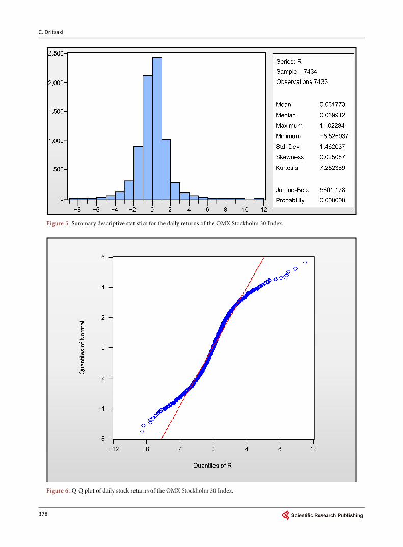
The summary of the descriptive statistics for the daily logarithmic stock index returns of the OMX Stockholm 30 Index is presented in Figure 5.

The results in Figure 5 show that the daily return rates do not follow normal distribution. In other words, the returns of the Stockholm stock market present positive asymmetry and kurtosis (leptokurtic), suggesting that the return distri-bution is a fat-tailed one. In Figure 6 the Q-Q plot is presented, which displays the quantiles of return data series against the quantiles of the normal distribu-tion.

C. Dritsaki

377

Figure 4. Correlogram of squared daily stock returns of the OMX Stockholm 30 Index.

The Q-Q plot, which displays the quantiles of return data series against the

quantiles of the normal distribution, shows that there is a low degree of fit of the empirical distribution to the normal distribution.

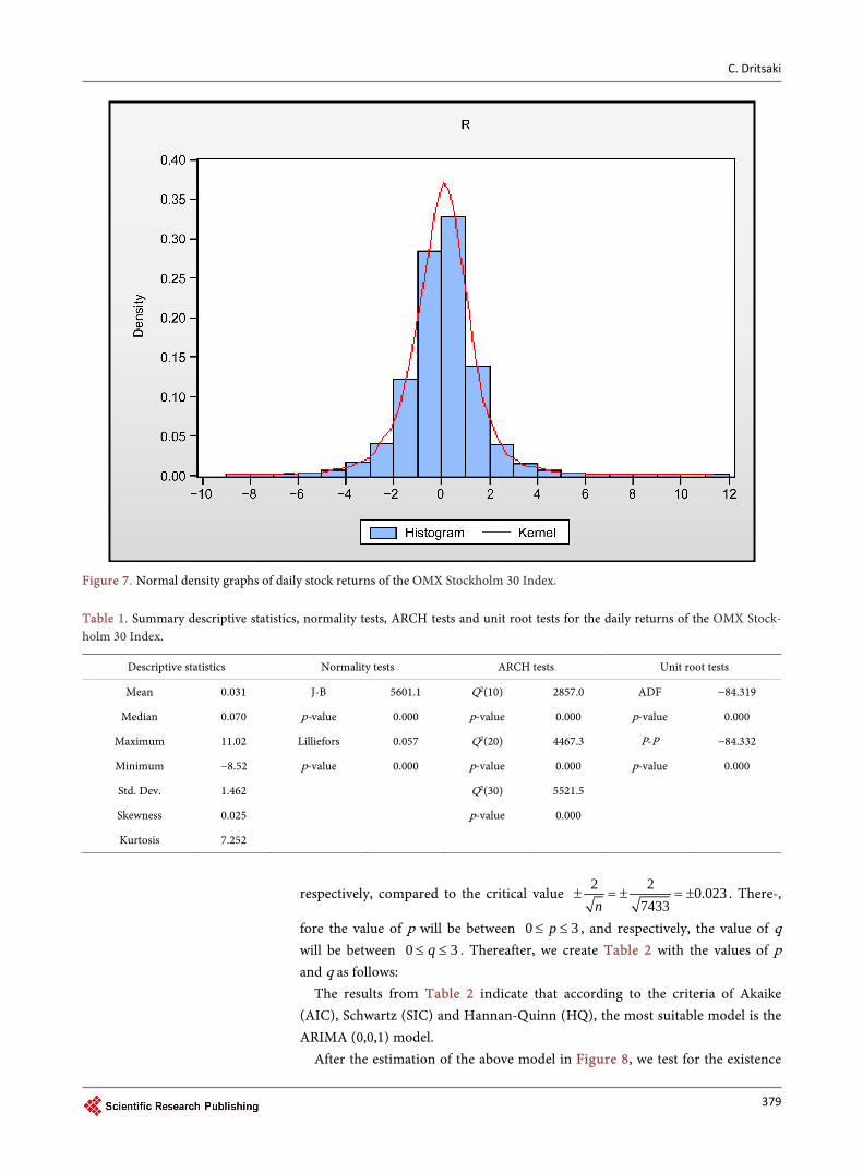
The leptokurtic behavior of the data is confirmed by the normal quintile and empirical density graph presented in Figure 7.

The summary of the descriptive statistics, normality tests, ARCH tests and unit root tests for the daily stock index returns of the OMX Stockholm 30 Index is presented in Table 1.

After the detection of series stationarity, we define the form of the ARMA (p, q) model from the correlogram of Figure 3. Parameters p and q can be deter-mined from partial autocorrelation coefficients and autocorrelation coefficients

C. Dritsaki

378

Figure 5. Summary descriptive statistics for the daily returns of the OMX Stockholm 30 Index.

Figure 6. Q-Q plot of daily stock returns of the OMX Stockholm 30 Index.

C. Dritsaki

379

Figure 7. Normal density graphs of daily stock returns of the OMX Stockholm 30 Index. Table 1. Summary descriptive statistics, normality tests, ARCH tests and unit root tests for the daily returns of the OMX Stock-holm 30 Index.

Descriptive statistics Normality tests ARCH tests Unit root tests

Mean 0.031 J-B 5601.1 Q2(10) 2857.0 ADF −84.319

Median 0.070 p-value 0.000 p-value 0.000 p-value 0.000

Maximum 11.02 Lilliefors 0.057 Q2(20) 4467.3 P-P −84.332

Minimum −8.52 p-value 0.000 p-value 0.000 p-value 0.000

Std. Dev. 1.462 Q2(30) 5521.5

Skewness 0.025 p-value 0.000

Kurtosis 7.252

respectively, compared to the critical value 2 2 0.0237433n

± = ± = ± . There-,

fore the value of p will be between 0 3p≤ ≤ , and respectively, the value of q will be between 0 3q≤ ≤ . Thereafter, we create Table 2 with the values of p and q as follows:

The results from Table 2 indicate that according to the criteria of Akaike (AIC), Schwartz (SIC) and Hannan-Quinn (HQ), the most suitable model is the ARIMA (0,0,1) model.

After the estimation of the above model in Figure 8, we test for the existence

C. Dritsaki

380

Table 2. Comparison of models within the range of exploration using AIC, SIC and HQ.

ARIMA model AIC SC HQ

(1,0,0) 3.5977 3.6005 3.5986

(2,0,0) 3.5977 3.6005 3.5986

(3,0,0) 3.5977 3.6005 3.5986

(1,0,1) 3.5977 3.6005 3.5986

(2,0,1) 3.5977 3.6005 3.5986

(3,0,1) 3.5977 3.6006 3.5987

(1,0,2) 3.5977 3.6006 3.5987

(2,0,2) 3.5977 3.6006 3.5987

(3,0,2) 3.5968 3.6033 3.5990

(1,0,3) 3.5968 3.6021 3.5986

(2,0,3) 3.5967 3.6032 3.5990

(3,0,3) 3.5977 3.6007 3.5987

(0,0,1) 3.5966 3.6004 3.5984

(0,0,2) 3.5977 3.6006 3.5987

(0,0,3) 3.5977 3.6007 3.5989

Figure 8. Estimation of the ARIMA (0, 0, 1) model.

C. Dritsaki

381

of conditional heteroscedasticity (ARCH(q) test) from the squared residuals of the above model. Figure 9 gives these results.

From the results of Figure 9 we can see that autocorrelation coefficients and partial autocorrelation coefficients are statistically significant. Consequently, the null hypothesis for the absence of ARCH or GARCH procedure is rejected.

5. Empirical Results

Since there are ARCH effects in the Stockholm stock return data, we can proceed with the estimation of the ARIMA(0,0,1)-GARCH models.

Figure 9. Q-statistics for the standardized squared residuals.

C. Dritsaki

382

First of all, we estimate the symmetric ARIMA(0,0,1)-GARCH(1,1) model with normal distribution, t-student distribution as well as the Generalized error distribution (GED). The estimation of parameters is done with the maximum li-kelihood method using the Broyden-Fletcher-Goldfarb-Shanno (BFGS) (see Press et al. [22]) algorithm which is a repeating method for solving non-linear optimization problems without constraint. The parameters (coefficients) of es-timated models and the residuals’ test of normality, autocorrelation and condi-tional heteroskedasticity are provided in Table 3. A higher log-likelihood value yields a better fit.

Table 3 gives both the estimation of parameters along with the value of the log-likelihood function as well as the residual tests of normality, autocorrelation and conditional heteroskedasticity. From the above table we point out that coef-ficients are statistically significant with all distributions. Also, there is no auto-correlation and conditional heteroskedasticity problem. Furthermore, the ARIMA(0,0,1)-GARCH(1,1) model has the largest value in logarithmic likelih-ood (LL) with t-student distribution. Thus, we can use this model for forecast-ing.

We proceed with the following asymmetric (non linear) GARCH models such as the ARIMA(0,0,1)-EGARCH (1,1) model as well as the ARIMA(0,0,1)-GJR- GARCH(1,1) model with the normal distribution, t-student distribution and Generalized error distribution (GED). The estimation of parameters is done with the Broyden-Fletcher-Goldfarb-Shanno (BFGS) algorithm Marquardt [1]. The parameters (coefficients) of estimated models and the residuals test of normality, autocorrelation and conditional heteroskedasticity are provided in Table 4.

From the results of Table 4 we can see that all the coefficients of non-linear GARCH models are statistically significant. These results show that asymmetry exists. Furthermore, diagnostics tests of non-linear GARCH models seem to be Table 3. Estimated symmetric GARCH models for the daily returns of the OMX Stock-holm 30 Index.

ARIMA(0,0,1)-GARCH(1,1)

Parameter Normal Student’s-t GED

ω 0.037(0.000) 0.025(0.000) 0.030(0.000)

α1 0.096(0.000) 0.095(0.000) 0.096(0.000)

β1 0.885(0.000) 0.894(0.000) 0.890(0.000)

D.O.F = 9.056 (0.000) PAR = 1.499(0.000)

Persistence 0.981 0.989 0.986

LL −12245.51 −12112.3 −12148.7

Jarque-Bera 2610.0(0.000) 3408.1(0.000) 2982.4(0.000)

ARCH(10) 2.783(0.986) 3.034(0.980) 2.911(0.983)

Q2( 30) 12.142(0.998) 16.335(0.980) 14.439(0.993)

Notes: 1. The persistence is calculated as α1 + β1 for the ARMA(0,0,1)-GARCH(1,1) model. 2. Values in parentheses denote the p-values. 3. LL is the value of the log-likelihood.

C. Dritsaki

383

Table 4. Estimated asymmetric GARCH models for the Daily Returns of the OMX Stockholm 30 Index.

ARIMA(0,0,1)-EGARCH(1,1)

Parameter Normal t-Student GED

Ω −0.111(0.000) −0.122(0.000) −0.118(0.000)

α1 0.158(0.000) 0.167(0.000) 0.163(0.000)

β1 0.975(0.000) 0.978(0.000) 0.977(0.000)

γ1 −0.088(0.000) −0.089(0.000) −0.087(0.000)

T-Dist.Dof 10.128(0.000) 1.546(0.000)

Persistence 0.975 0.978 0.977

LL −12159.04 −12044.66 −12082.75

Jarque-Bera 2199.27(0.000) 2601.59(0.000) 2397.07(0.000)

ARCH(10) 4.521(0.920) 3.162(0.977) 3.647(0.961)

Q2(30) 12.667(0.998) 13.641(0.995) 12.869(0.997)

ARIMA(0,0,1)-GJR-GARCH(1,1)

Parameter Normal t-Student GED

Ω 0.040(0.000) 0.033(0.000) 0.036(0.000)

α1 0.023(0.000) 0.026(0.000) 0.025(0.000)

β1 0.891(0.000) 0.890(0.000) 0.890(0.000)

γ1 0.127(0.000) 0.131(0.000) 0.128(0.000)

T-Dist.Dof 10.198(0.000) 1.555(0.000)

Persistence 0.9775 0.9815 0.979

LL −12155.06 −12042.88 −12080.43

Jarque-Bera 2105.14(0.000) 2534.87(0.000) 2308.25(0.000)

ARCH(10) 3.521(0.966) 4.555(0.918) 3.989(0.947)

Q2(30) 12.492(0.998) 15.569(0.986) 13.923(0.995)

Notes: 1. The persistence is calculated as 1β for ARIMA(0,0,1)-EGARCH(1,1) model, and 1 1 12α γ β+ + for ARIMA(0,0,1)-GJR-GARCH(1,1) model. 2. Values in parentheses denote the p-values. 3. LL is the value of the log-likelihood.

satisfactory. Also, the results from the models show that Q-statistics for the standardized squared residuals and the ARCH-LM test are insignificant with high p values. From the above table we can see that ARIMA(0,0,1)-GJR- GARCH(1,1) model has the largest logarithmic likelihood (LL) value with t-student distribution. Thus, this model can be used for forecasting.

5.1. Asymmetric and Leverage Effects

Asymmetry and leverage effects results are examined for non-linear variances of ARIMA(0,0,1)-EGARCH(1,1) and ARIMA(0,0,1)-GJR-GARCH(1,1) models from three different distributions. Since the coefficients are statistically signifi-cant in all cases, asymmetry exists. Positive signs of the coefficients on the

C. Dritsaki

384

ARIMA(0,0,1)-GJR-GARCH(1,1) models as well as negative signs on the ARIMA(0,0,1)-EGARCH(1,1) models indicate that there are leverage effects. In addition, bad news has more impact on volatility than good news in all distribu-tions that we used. In the following Table 5, we present the models with the three distributions indicating that bad news have more impact on volatility. For example, on the ARIMA(0,0,1)-GJR-GARCH(1,1) model and t-student the effect of bad news on conditional volatility is 6.03 times higher than good news.

5.2. Test of Asymmetries

In order to examine if an asymmetric model is suitable for forecasting, Engle and Ng [15] created a test known as the sign and size bias test defining if an asym-metric model is suitable for the examined series or to what extent the symmetric GARCH model is considered adequate. The Engel-Ng [15] test is usually applied to the residuals of a GARCH fit to the returns data. The sign and size bias test is based on the significance of b1 coefficient of the following regression:

20 1 , 1t̂ i t tb b D vε −

−= + + (15)

where 2t̂ε are the squared residuals from the symmetric GARCH model.

, 1i tD−− is a dummy variable which takes the value 1 if t iε − is negative and 0

otherwise, and gives the slope dummy value.

tv is an i.i.d. error term. (see Dutta [14]). If b1 coefficient is statistically significant in positive and negative changes rela-

tively to conditional variance then there is asymmetry on the GARCH model. A test for sign bias can also be conducted using the following regression:

20 1 1 1t̂ t t tb b D vε ε−

− −= + + (16)

Like regression (15), the statistical significance of b1 coefficienton regression (16) indicates that the size of a shock will have an asymmetric impact on volatil-ity. Regression (16) tests the negative bias size. For the positive bias size we use the following regression: (see Dutta [14])

( )20 1 1 1ˆ 1t t t tb b D vε ε−

− −= + − + (17)

A joint test can be conducted through defining 1tD+− as 11 tD−

−− which indi-cates a positive size bias. The joint test for positive sign bias and positive or neg-ative size bias is presented on the following regression: Table 5. The magnitude of news impact on volatility.

ARIMA(0,0,1)-EGARCH(1,1) ARIMA(0,0,1)-GJR-GARCH(1,1)

Normal t-Student GED Normal t-Student GED

Bad News 1.088 1.089 1.089 0.150 0.157 0.153

Good News 1.012 0.911 0.913 0.023 0.026 0.025

Notes: The asymmetry is calculated as 11 γ− , and 11 γ+ for the ARIMA(0,0,1)-EGARCH(1,1) model,

1 1α γ+ , and 1α for the ARIMA(0,0,1)-GJR-GARCH(1,1) model.

C. Dritsaki

385

20 1 1 2 1 1 3 1 1t̂ t t t t t tb b D b D b D vε ε ε− − +

− − − − −= + + + + (18)

The significance of b1 coefficient of regression (17) shows the existence of sign bias where positive and negative changes have different consequences in volatil-ity compared to the symmetric GARCH model. On the other hand, the signific-ance of b2 and b3 coefficients of regression (18) indicates not only size bias but also if the size of change is significant. The test follows a χ2 distribution with de-grees of freedom equal to 3. The joint test statistic is given from the formula TR2. The null hypothesis for the joint test is that there is no asymmetric result. (see Brooks, [23], pp. 474-475). Table 6 presents the results of the asymmetry and volatility tests.

The results of Table 6 show that the sign bias test is statistically significant on both models. Thus, there is asymmetry. This result is also confirmed from two size bias tests having large statistical significance. Also, from the results of the above table we can see that the size effect of bad news is stronger than that of good news.

5.3. Likelihood Ratio Tests

The Likelihood ratio (LR) tests consist of estimations on two models, (an unre-stricted model and a restricted one). The null hypothesis that is examined is

0 1: 0H γ = . The maximized values of log-likelihood function (LLF) are used on this test according to the following:

( ) ( )22 r uLR LLF LLF mχ= − − → (19)

where

rLLF is the value of maximum likelihood function from the constrained model

uLLF is the value of maximum likelihood function from the unconstrained model

m the number of constraints. The Likelihood ratio (LR) tests follow asymptotically χ2 distribution with m

degrees of freedom. Table 7 presents the maximized values from all estimated models with the corresponding distributions. Table 6. Tests of asymmetries.

ARIMA(0,0,1)-EGARCH(1,1) ARIMA(0,0,1)-GJR-GARCH(1,1)

Normal t-Stud. GED Normal t-Stud. GED

Sign bias 0.030* 0.056* 0.039* 0.203* 0.054* −0.053*

Negative size bias −0.265* −0.055* −0.015* −0.684* −0.048* −0.030*

Positive size bias 0.331* 0.043* 0.111* 0.039 0.036* 0.019*

Joint test (F-test) 2614.8 853.4 9212.3 1115.06 432.36 13409.3

p-value (0.000) (0.000) (0.000) (0.000) (0.000) (0.000)

Notes: 1. (*) denotes significance at the (1%); 2. The t-statistics for the sign bias, negative size bias and pos-itive size bias tests are those of coefficient b1 in regression (15), (16) and (17), respectively. 3. The F-statistic is basedon regression (18). 4. Values in parentheses denote the p-values.

C. Dritsaki

386

Table 7. Likelihood-ratio test results.

LLFr LLFu LR

ARIMA(0,0,1)-GARCH(1,1) Normal −12245.51

t-Student −12112.3

GED −12148.7

ARIMA(0,0,1)-EGARCH(1,1) Normal −12159.04 172.94*

t-Student −12044.66 135.28*

GED −12082.75 131.9*

ARIMA(0,0,1)-GJR-GARCH(1,1) Normal −12155.06 180.9*

t-Student −12042.88 138.84*

GED −12080.43 136.5*

Note: (*) denotes significance at the (1%) level, LLFr is the value from maximum likelihood function from the constrained model, LLFu is the value from maximum likelihood function from the unconstrained model and LR is Likelihood ratiotest.

The results from Table 7 show that null hypothesis is rejected so asymmetry

exists. Thus, we can use both models of forecasting due to existence of asymme-try (Engle and Ng, and LR test). Furthermore, the negative value of 1γ coeffi-cient on the ARIMA(0,0,1)-EGARCH(1,1) model and the positive value of 1γ coefficient on the ARIMA(0,0,1)-GJR-GARCH(1,1) model denote the presence of leverage.

6. Forecasting the Volatility of the Stockholm Stock Exchange Index Returns ex Post

In this section we present the forecasting results from the two asymmetric mod-els. In our paper we forecast for future values on rate of return and volatility on the Stockholm stock market using the static1-step ahead method based on esti-mated parameters of the two asymmetric models. The last 434 series observa-tions were used for an ex-post forecast, with the main focus on the forecast of volatility. In the literature, a variety of statistics has been used which evaluates and compares the forecasts of returns. The optimal forecasting value is evaluated through Mean Squared Error. Other statistical indices usually used for the return of forecasting are the Mean Absolute Error (MAE), the Root Mean Square Error (RMSE), the Mean Absolute Percentage Error (MAPE) and the (Theil U-Theil index [24]). The lower the values of the RMSE, MAE and MAPE indices, the better the forecast of models. Figure 10 and Figure 11 of the two models for the period we analyze are given below:

The above figures show that estimation intervals are stable on both models. However, there are some indices that help us to test the forecast of a model. The first one is referred to as the Mean Square Error. According to Patton [25] this criterion is the most powerful for the evaluation of models. However, the mean square error has some constraints on the forecasting of variance. According to Vilhelmsson [26], this index is sensitive to outliers. So, Vilhelmsson suggests the

C. Dritsaki

387

Figure 10. Ex-post forecast of the volatility of the Stockholm Stock Exchange index returns (ARIMA(0,0,1)-EGARCH(1,1).

Figure 11. Ex-post forecast of the volatility of the Stockholm Stock Exchange index returns (ARIMA(0,0,1)-GJR-GARCH(1,1).

C. Dritsaki

388

mean absolute error index which is more robust to outliers. According to the Mean Absolute Error (MAE), the Root Mean Square Error(RMSE) and Mean Absolute Percentage Error (MAPE), the ARIMA(0,0,1)-EGARCH(1,1) model provides more exact forecasts on the returns of the Stockholm stock market.

7. Conclusions

The modeling and forecasting of volatility in financial markets used to be a fun-damental issue for many researchers. The importance of this problem increased over the last years as there is upheaval in the financial world. The aim of this paper is to compare various volatility models and forecast for future values re-garding the rate of return and volatility of the Stockholm stock market using 1-step ahead. Measuring the period from 30 September 1986 until 11 May 2016 and using as a sample 7,434 daily observations for different models we con-cluded that the asymmetric models give better results on the returns and volatil-ity of the Stockholm stock market. More specifically, we estimated the symme-tric ARIMA(0,0,1)-GARCH(1,1) model, as well as the asymmetric models ARIMA(0,0,1)-EGARCH(1,1) and ARIMA(0,0,1)-GJR-GARCH(1,1) models with different residual distributions. The analysis of estimations indicated that t-student distribution is considered the most suitable on the estimation of para-meters for all models. These results are in accordance with the empirical works by (Hamilton and Susmel [27]), (Poon and Granger [28]) and many others do-cumented conditional non-Gaussianities in financial data. Moreover, an effort was made to test the asymmetric response of volatility on the positive and nega-tive changes of models. The results of our paper, as far as the asymmetric tests are concerned, showed that negative changes are more frequent and more po-werful (robust) on the returns of the Stockholm stock market.

To sum up, the results of our paper confirm previous findings that GARCH models with normal errors do not seem to fully capture the leptokurtosis in em-pirical time series (see, e.g. Kim and White [29]). Contrary to t-student distribu-tion and GED, which provide a better frame on conditional volatility, we can better test the time-varying heteroskedasticity, skewness and kurtosis of the se-ries. This is accomplished by allowing the parameters of the two distributions to vary through time. Finally, the asymmetric models appear to better formulate the different responses to different past shocks and to explain conditional vola-tility.

References [1] Marquardt, D.W. (1963) An Algorithm for Least Squares Estimation of Nonlinear

Parameters. Journal of the Society for Industrial and Applied Mathematics, 11, 431- 441. https://doi.org/10.1137/0111030

[2] Engle, R.F. (1982) Autoregressive Conditional Heteroscedasticity with Estimates of the Variance of UK Inflation. Econometrica, 50, 987-1008. https://doi.org/10.2307/1912773

[3] Bollerslev, T. (1986) Generalized Autoregressive Conditional Heteroskedasticity. Journal of Econometrics, 31, 307-327.

C. Dritsaki

389

https://doi.org/10.1016/0304-4076(86)90063-1

[4] Black, F. (1976) Studies in Stock Price Volatility Changes of the Nominal Excess Return on Stocks. Proceedings of the American Statistical Association, Business and Economics Statistics Section, 177-181.

[5] Nelson, D.B. (1991) Conditional Heteroskedasticity in Asset Returns: A New Ap-proach. Econometrica, 59, 347-370. https://doi.org/10.2307/2938260

[6] Glosten, L.R., Jagannathan, R. and Runkle, D.E. (1993) On the Relation between the Expected Value and the Volatility of the Nominal Excess Return on Stocks. The Journal of Finance, 48, 1779-1801. https://doi.org/10.1111/j.1540-6261.1993.tb05128.x

[7] Donaldson, R.G. and Kamstra, M. (1997) An Artificial Neural Network—GARCH Model for International Stock Return Volatility. Journal of Empirical Finance, 4, 17-46. https://doi.org/10.1016/s0927-5398(96)00011-4

[8] Nam, K., Pyun, C.S. and Arize, C.A. (2002) Asymmetric Mean-Reversion and Con-trarian Profits: ANSTGARCH Approach. Journal of Empirical Finance, 9, 563-588. https://doi.org/10.1016/S0927-5398(02)00011-7

[9] Tudor, C. (2008) Modeling Time Series Volatilities Using Symmetrical GARCH Models. The Romanian Economic Journal, 30, 183-208.

[10] Panait, I. and Slavescu, E.O. (2012) Using Garch-in-Mean Model to Investigate Vo-latility and Persistence at Different Frequencies for Bucharest Stock Exchange dur-ing 1997-2012. Theoretical and Applied Economics, 19, 55-76.

[11] Gao, Y., Zhang, C. and Zhang, L. (2012) Comparison of GARCH Models Based on Different Distributions. Journal of Computers, 7, 1967-1973. https://doi.org/10.4304/jcp.7.8.1967-1973

[12] Dutta, A. (2014) Modelling Volatility: Symmetric or Asymmetric GARCH Models? Journal of Statistics: Advances in Theory and Applications, 12, 99-108.

[13] Bollerslev, T., Chou, R.Y. and Kroner, K.F. (1992) ARCH Modeling in Finance: A Review of the Theory and Empirical Evidence. Journal of Econometrics, 52, 5-59. https://doi.org/10.1016/0304-4076(92)90064-X

[14] Poon, S.H. and Granger C.W.J. (2003) Forecasting Volatility in Financial Markets: A Review. Journal of Economic Literature, 41, 478-539. https://doi.org/10.1257/.41.2.478

[15] Engle, R.F. and Ng, V.K. (1993) Measuring and Testing the Impact of News on Vo-latility. Journal of Finance, 48, 1749-1778. https://doi.org/10.1111/j.1540-6261.1993.tb05127.x

[16] Greene, W.H. (2012) Econometric Analysis. 7th Edition, Prentice Hall, Upper Sad-dle River.

[17] Brooks, C., Clare, A.D. and Persand G. (2000) A Word of Caution on Calculating Market Based Minimum Capital Risk Requirements. Journal of Banking and Finance, 24, 1557-1574. https://doi.org/10.1016/S0378-4266(99)00092-8

[18] Vilasuso, J. (2002) Forecasting Exchange Rate Volatility, Economics Letters, 76, 59- 64. https://doi.org/10.1016/S0165-1765(02)00036-8

[19] Bollerslev, T. (1987) Conditionally Heteroskedastic Time Series Model for Specula-tive Prices and Rates of Return. Review of Economics and Statistics, 69, 542-547. https://doi.org/10.2307/1925546

[20] Ljung, G. and Box, G. (1978) On a Measure of Lack of Fit in Time Series Models. Biometrika, 65, 297-303. https://doi.org/10.1093/biomet/65.2.297

[21] Ljung, G. and Box, G. (1979) The Likelihood Function of Stationary Autoregres-

C. Dritsaki

390

sive-Moving Average Models. Biometrika, 66, 265-270. https://doi.org/10.1093/biomet/66.2.265

[22] Press, W., Flannery, B., Teukolsky, S. and Vettering, W. (1988) Numerical Recipes in C. Cambridge University Press, New York.

[23] Brooks, C. (2008) Introductory Econometrics for Finance. 2nd Edition, Cambridge University Press, New York. https://doi.org/10.1017/CBO9780511841644

[24] Theil, H. (1961) Economic Forecasts and Policy. North-Holland Publishing Com-pany, Amsterdam.

[25] Patton, A. (2006) Volatility Forecast Comparison Using Imperfect Volatility Prox-ies. University of Technology, Sydney.

[26] Vilhelmsson, A. (2006) Garch Forecasting Performance under Different Distribu-tion Assumptions. Journal of Forecasting, 25, 561-578. https://doi.org/10.1002/for.1009

[27] Hamilton, J.D. and Susmelb, R. (1994) Autoregressive Conditional Heteroskedastic-ity and Changes in Regime. Journal of Econometrics, 64, 307-333. https://doi.org/10.1016/0304-4076(94)90067-1

[28] Poon, S.H. and Granger, C. (2003) Forecasting Volatility in Financial Markets: A Review. Journal of Economic Literature, 41, 478-539. https://doi.org/10.1257/.41.2.478

[29] Kim, T.H. and White, H. (2004) On More Robust Estimation of Skewness and Kur-tosis. Finance Research Letters, 1, 56-73. https://doi.org/10.1016/S1544-6123(03)00003-5

Submit or recommend next manuscript to SCIRP and we will provide best service for you:

Accepting pre-submission inquiries through Email, Facebook, LinkedIn, Twitter, etc. A wide selection of journals (inclusive of 9 subjects, more than 200 journals) Providing 24-hour high-quality service User-friendly online submission system Fair and swift peer-review system Efficient typesetting and proofreading procedure Display of the result of downloads and visits, as well as the number of cited articles Maximum dissemination of your research work

Submit your manuscript at: http://papersubmission.scirp.org/ Or contact jmf@scirp.org