An ELLAM Scheme for Advection-Dispersion Equations

in Two Dimensions�

Hong Wang y Helge K. Dahle z Richard E. Ewing x Magne S. Espedal z

Robert C. Sharpley y Shushuang Man y

Abstract We develop an ELLAM (Eulerian-Lagrangian localized adjoint method) scheme to solve two-dimensional advection-dispersion equations with all combinations of in ow and out ow Dirichlet, Neumann,

and ux boundary conditions. The ELLAM formalism provides a systematic framework for implementation ofgeneral boundary conditions, leading to mass-conservative numerical schemes. The computational advantages

of the ELLAM approximation have been demonstrated for a number of one-dimensional transport systems;practical implementations of ELLAM schemes in multiple spatial dimensions that require careful algorithmdevelopment are discussed in detail in this paper. Extensive numerical results are presented to compare the

ELLAM scheme with many widely used numerical methods and to demonstrate the strength of the ELLAMscheme.

1 Introduction

Many di�cult problems arise in the numerical simulation of advection-dispersion equations,which describe the transport of solutes in groundwater and surface water, the displace-ment of oil by uid injection in oil recovery, the movement of aerosols and trace gases inthe atmosphere, and miscible uid ow processes in many other applications. In indus-trial applications, these equations are commonly discretized via �nite di�erence methods(FDM) or �nite element methods (FEM) in large-scale simulators. Because of the enormoussize of many �eld-scale applications, large grid-spacings must be used in the simulations.When physical dispersion dominates the transport process, these methods perform fairlywell. However, when advection dominates the transport process, these methods su�er fromserious numerical di�culties. Centered FDM (in space or time) and corresponding FEMoften yield numerical solutions with excessive oscillations. The classical space-upwinded (orbackward-in-time) schemes can greatly suppress the oscillations, but they tend to generatenumerical solutions with severe damping or a combination of both. Recent developments ine�ectively solving advection-dispersion equations have generally been along one of the twoapproaches: Eulerian or characteristic methods. Eulerian methods use a �xed spatial gridsuch as optimal test function methods of Christie and coworkers (1976), Barrett and Morton

�This research was supported in part by DE-FG03-95ER25263 and DE-FG05-95ER25266, by ONR N00014-94-

1-1163, by funding from the Institutes for Scienti�c Computation at Texas A&M University, and by funding from

VISTA, a research cooperation between Statoil and the Norwegian Academy of Science and Letters.yDepartment of Mathematics, University of South Carolina, Columbia, South Carolina 29208, USAzDepartment of Mathematics, University of Bergen, Johs. Brunsgt. 12, N-5007, Bergen, Norway.xInstitute for Scienti�c Computation, Texas A&M University, College Station, Texas 77843-3404, USA

1

(1984), Celia et al. (1989), and Bank et al. (1990). These methods attempt to minimizethe error in approximating spatial derivatives and yield an upstream bias in the resultingnumerical schemes. Hence, they are susceptible to time truncation errors that introducenumerical dispersion and the restrictions on the size of the Courant number, and they tendto be ine�ective for transient advection-dominated problems. They generally require smalltime steps for reasons of accuracy, because the time truncation error depends on high-ordertime derivatives of the solutions that are large when a sharp front passes by. Other Eulerianmethods, such as the Petrov-Galerkin FEM of Westerink and Shea (1989), Bouloutas andCelia (1991), and the total variation diminishing scheme of Cox and Nishikawa (1991), at-tempt to reduce the overall truncation error by using negative temporal numerical dispersionto cancel positive spatial numerical dispersion. Therefore, they also su�er from the Courantnumber restrictions. Also, included in the class of Eulerian methods is the streamline dif-fusion �nite element method (SDFEM) of Hughes, Brooks, and Johnson, et al. (Hughesand Brooks 1979, Brooks and Hughes 1982, Hughes and Mallet 1986, Hughes 1995, Hansboand Szepessy 1990, Hansbo 1992, Johnson and N�avert 1981, Johnson and Pitk�aranta 1986,Johnson 1987, Johnson et al. 1990, Johnson and Szepessy 1995, Zhou 92, and Zhou 95).Via a framework of space-time FEM, the SDFEM uses piecewise polynomial trial/test func-tions over a partition on a space-time domain (spatial domain � current time interval). Byde�ning the test functions delicately, the SDFEM adds a numerical dispersion only in thedirection of characteristics (streamline) to suppress the oscillation and does not introduceany cross-wind di�usion. Therefore, this method possesses many physical and numericaladvantages other Eulerian methods do not have. However, this method contains a unde-termined parameter in the test functions that needs to be chosen very carefully to obtainaccurate numerical results. If the parameter is chosen too small, the numerical solutions willexhibit oscillations. But if it is too large, the SDFEM will introduce excessive numericaldispersion and seriously smear the numerical solutions. Unfortunately, an optimal choiceof the parameter is not clear and is heavily problem-dependent. Moreover, the number ofunknowns are doubled compared to many standard Eulerian or characteristic methods.

Because of the hyperbolic nature of advective transport, characteristic analysis is nat-ural to aid in the solution of advection-dispersion equations and has led to many relatedapproximation techniques, including the method of characteristics of Garder et al. (1964),Pinder and Cooper (1970), Benque and Ronat (1982), and Hervouet (1986); the charac-teristic Galerkin method of Varoglu and Finn (1980); the Eulerian-Lagrangian method ofNeuman (1981); the transport-di�usion method of Pironneau (1982); the modi�ed method ofcharacteristics of Douglas and Russell (1982), and Ewing et al. (1983); the operator-splittingmethod of Espedal and Ewing (1987), Wheeler and Dawson (1988), and Dahle et al. (1990);and the Lagrangian-Galerkin method of Morton and coworkers (1988). Characteristic meth-ods e�ectively solve the advective component by a characteristic tracking algorithm and treatthe di�usive term separately. These methods have signi�cantly reduced the time truncationerrors in the Eulerian methods, have generated accurate numerical solutions even if largetime steps are used, and have eased the Courant number restrictions of Eulerian methods.Problems with many characteristic methods arise in the areas of rigorously treating bound-ary uxes when characteristics intersect in ow or out ow boundaries and of maintaining

2

mass conservation.

The Eulerian-Lagrangian localized adjoint method (ELLAM) was �rst introduced byCelia et al. (1990), Russell (1990), and Herrera et al. (1993) for the solution of one-dimensional (constant-coe�cient) advection-di�usion equations. The ELLAM formalismprovides a general characteristic solution procedure for advection-dominated problems, andit presents a consistent framework for treating general boundary conditions and maintainingmass conservation. Subsequently, Russell and Trujillo (1990), Wang (1992), and Wang et

al. (1992) derived di�erent ELLAM schemes for one-dimensional linear variable-coe�cientadvection-di�usion equations with general in ow and out ow boundary conditions, based ondi�erent (forward or backward) techniques for the tracking of characteristics of the velocity�eld. Celia and Ferrand (1993), and Healy and Russell (1993) extended ELLAM to a �nite-volume setting for one-dimensional advection-di�usion equations. Ewing (1991) and Dahleet al. (1995) addressed the ELLAM techniques for one-dimensional nonlinear advection-di�usion equations. Ewing and Wang (1991, 1993a, 1993b) also developed ELLAM schemesfor the solution of one-dimensional advection-reaction equations with an initial conditionand in ow boundary condition. In addition, Celia and Zisman (1990), and Ewing and Wang(1993c,1994) generalized ELLAM schemes for one-dimensional advection-di�usion-reactiontransport equations. Wang et al. (1995a), and V�ag and coworkers applied ELLAM schemesto solve the systems of one-dimensional reactive transport problems from bioremediationand other applications (V�ag et al.).

While the computational advantages of ELLAM approximations have been demonstratedfor one-dimensional advection-dominated problems by the extensive research mentionedabove, practical implementation of ELLAM schemes in multiple spatial dimensions requirescareful algorithm development, in which some research has been carried out in this direction.Russell and Trujillo (1990) addressed various issues in multidimensional ELLAM schemes.Wang (1992) developed an ELLAM simulator to solve two-dimensional linear advection-dispersion equations with general in ow and out ow boundary conditions by combiningforward and backward tracking algorithms. Theoretically optimal-order error estimates forthe derived scheme were also proved, and various numerical experiments were performed.Some of these results were reported in Ewing and Wang (1993a,1993b). By using an explicitmapping of the �nite elements at the current time level to the spatial grids at the previoustime, Binning and Celia (Binning 1994, Binning and Celia 1996) reported on a �nite-volumeELLAM formulation for unsaturated transport in two dimensions. Relations and di�erencesbetween the two approaches are discussed in some detail in Section 4 of this paper. Celia(1994) also explored the development of an ELLAM scheme for three-dimensional advection-dispersion equations.

A di�erent but related method is the `characteristic-mixed �nite-element' method ofArbogast et al. (1992), Yang (1992), and Arbogast andWheeler (1995), which uses piecewise-constant space-time test functions. As with the standard mixed method, a coupled systemresults for both the concentration and the di�usive ux. The theoretically proven errorestimate is (O(�x)3=2) for grid size �x, which is suboptimal by a factor O((�x)1=2). For

3

ELLAM schemes with piecewise linear trial/test functions for one-dimensional advection-di�usion equations, advection-di�usion-reaction equations, and �rst-order advection-reactionequations, optimal-order error estimates of O((�x)2) have been proven by Ewing and Wang(1991,1993a,1996), Wang et al. (1995a), and Wang and Ewing (1995).

In this paper, we develop an ELLAM scheme for the solution of two-dimensional linearvariable-coe�cient advection-dispersion equations with general in ow and out ow boundaryconditions based on the approach presented in Wang (1992). The rest of the paper is asfollows: In Section 2, we present a space-time variational formulation. In Section 3, wederive an ELLAM numerical scheme. In Section 4, we discuss implementational issues. InSection 5, we describe the results of the numerical experiments and compare the performanceof the ELLAM scheme with the many other well-developed, extensively studied numericalmethods.

2 Variational Formulation

A general linear, variable-coe�cient advection-dispersion partial di�erential equation in twodimensions can be written as follows:

Lu(x; t) � (R(x; t)u)t +r � (V(x; t)u �D(x; t)ru) = f(x; t);

(x; t) = (x; y; t) 2 � = � J;(2:1)

where ut =@u@t, ru = (@u

@x; @u@y)T , is a spatial domain, J = [0; T ] is a time interval. The

nomenclature is such that R(x; t) is a retardation coe�cient, V(x; t) = (V1(x; t); V2(x; t))is a uid velocity �eld, D(x; t) = (Dij(x; t))

2i;j=1 is a di�usion-dispersion tensor, f(x; t) is

a given forcing function, and u(x; t) is the solute concentration of a dissolved substance.Mathematically, R has positive lower and upper bounds, D(x; t) is a symmetric and positivede�nite matrix with uniform lower and upper bounds that are independent of (x; t).

Let the space-time boundary � = @ � J be decomposed as the union of an in owboundary �(I), an out ow boundary �(O), and a no ow boundary �(N) (i.e., � = �(I)[�(O)[�(N)). In general, an in ow boundary during one time period might become an out ow ora no ow boundary in the next time period or verse versa. At �(I) or �(O), one of Dirichlet,Neumann, or Robin ( ux) boundary conditions may be imposed by setting, respectively,

u(x; t) = g(i)1 (x; t); (x; t) 2 �(i);

�Dru(x; t) � n = g(i)2 (x; t); (x; t) 2 �(i);

(Vu �Dru)(x; t) � n = g(i)3 (x; t); (x; t) 2 �(i);

(2:2)

where n = n(x) is the outward unit normal, i = I or O represents the in ow or out owboundary, respectively. A no ow boundary condition is speci�ed at �(N) by

(Vu�Dru)(x; t) � n = 0; (x; t) 2 �(N): (2:3)

4

In addition to the boundary conditions, an initial condition u(x; 0) = u0(x) is needed toclose Equation (2.1).

The ELLAM formalism uses a time-marching algorithm. Let Nt be a positive integer.We de�ne a partition of time interval J = [0; T ] by

0 = t0 < t1 < t2 < : : : < tn < : : : < tNt�1 < tNt= T:

With space-time test functions w that vanish outside �n � �Jn with Jn � (tn�1; tn] andare discontinuous in time at time tn�1, one can write a space-time variational formulationfor Equation (2.1) as follows:Z

(R u w)(x; tn) dx+

Z�n

rw � (Dru) dxdt

+Z�n

(Vu�Dru) � n w dS �Z�n

u (R wt +V � rw) dxdt

=Z(R u w)(x; t+n�1) dx+

Z�n

f w dxdt;

(2:4)

where �n = @� Jn and w(x; t+n�1) = limt!t+

n�1

w(x; t).

In the ELLAM framework, one should de�ne the test functions w to satisfy the equationRwt+V �rw � 0, so the last term on the left-hand side of Equation (2.4) vanishes. However,in general one cannot track characteristics exactly for a variable-velocity �eld. Nevertheless,this adjoint term should be small if one can track the characteristics reasonably well, and thetest functions are constant along the approximate characteristics. In fact, we have provedan optimal-order convergence rate for the derived ELLAM scheme even if a one-step Euleralgorithm is used in the characteristic tracking and this adjoint term is dropped (Wang 1992,Ewing and Wang 1996). To conserve mass, all the basis of test functions should sum to one(Celia et al. 1990). The scheme developed in this paper satis�es this condition. In this casedropping the last term on the left-hand side does not a�ect mass conservation since thatterm vanishes if w � 1 (Russell and Trujillo 1990, Wang 1992).

We are now in a position to rewrite Equation (2.4). Given a point (�x; �t), with �t 2 [tn�1; tn],we consider the initial-value problem for the ordinary di�erential equation

dx

dt= VR(x; t) �

V(x; t)

R(x; t);

x(�t) = �x;

(2:5)

which tracks the characteristics from (�x; �t). We denote the solution of this equation at time� 2 Jn by X(�; �x; �t) (Healy and Russell 1993). This notation can refer to tracking eitherforward or backward in time. In particular, we de�ne

x� = X(tn�1;x; tn);

~x = X(tn;x; tn�1):(2:6)

5

Thus, (x; tn) backtracks to (x�; tn�1) and (x; tn�1) tracks forward to (~x; tn). In the numerical

scheme, an exact tracking is preferred whenever possible. However, it is impractical in mostapplications. In practice, one can use either a one-point Euler quadrature, a multiple micro-time-step tracking within a global time step, or a Rungle-Kutta quadrature in the trackingof characteristics. Note that in many applications, Equation (2.1) is usually coupled with anassociated potential or pressure equation, whose solution is often obtained via the mixed �niteelement method. In this case, a Raviart-Thomas space is often used for the velocity �eld,which is calculated at each cell interface. Within each cell, V1(x; t) (or V2(x; t)) is piecewiselinear (or constant) in the x direction and piecewise constant (or linear) in the y direction.Under the assumption that the velocity �eld is steady, a semi-analytical technique has beendeveloped by Pollock (1988), Schafer-Perini and Wilson (1991), and Heally and Russell(1993), to track the characteristics on a cell-by-cell basis. Recently, Lu (1994) extendedthis semi-analytical approach to nonsteady velocity �elds where velocity is assumed to varylinearly in time within each time interval.

To accurately measure the time period taken for a particle from the previous time levelor the in ow boundary to the current time level or the out ow boundary, we introduce somespace-time location-dependent time steps. For any x 2 at time tn, we de�ne a time step�t(I)(x) to be �t(I)(x) = �t � tn � tn�1 if the characteristic X(�;x; tn) does not backtrackto the space-time boundary �n during the time period Jn (This case is illustrated by pointA at time tn in Figure 1), and �t(I)(x) = tn � t�(x) otherwise (This case is deomnstratedby point B at tn in Figure 1), where t�(x) 2 Jn is the time when X(�;x; tn) intersectsthe boundary �n (i.e, X(t�(x);x; tn) 2 �n). Similarly, for any (x; t) 2 �(O)n , we de�ne�t(O)(x; t) = t � tn�1 if the characteristic X(�;x; t) does not intersect �n during the timeperiod [tn�1; t] (This case is shown by point C on the sapce-time boundary y = 0 in Figure1), and �t(O)(x; t) = t � t�(x; t) otherwise (This case is represented by point D on thespace-time boundary y = 0 in Figure 1), where t�(x; t) 2 [tn�1; t] is the time when X(�;x; t)intersects �n (i.e X(t�(x; t);x; t) 2 �n).

By enforcing the backward Euler quadrature at the current time tn and at the out owspace-time boundary �(O)n , we approximate the space-time volume integral of the source term(the second term on the right-hand side) in Equation (2.4) by an integral at time tn andone at �(O)n by following the characteristics. Here �(i)n = �(i) \ Jn (i = I;O;N) representsthe space-time in ow, out ow, and no ow boundaries during the time interval Jn. To avoidconfusion in the following derivation, we replace the dummy variables x 2 and t 2 Jnin this term by y 2 and � 2 Jn. Thus,

R�n

f w(x; t) dxdt =R�n

f w(y; �) dyd�. Let

�(O)n � �n be the set of points in the space-time strip �n that will ow out of �n during

the time interval Jn. We decompose �n to be the union of �(O)n and �n � �(O)

n . For any(y; �) 2 �n��(O)

n , there exists a point x 2 such that x = X(tn;y; �). Thus, we can invertthis relation to obtain y = X(�;x; tn). Similarly, for any (y; �) 2 �(O)

n , there exists a pair(x; t) 2 �(O)n such that y = X(�;x; t). By splitting the space-time volume integral on �n asone on �n � �(O)

n and one on �(O)n and applying the backward Euler quadrature at time tn

6

for the �rst and at boundary �(O)n for the second, we obtain the following equation

Z�n

f(y; �)w(y; �) dyd�

=Z�n��

(O)n

f(y; �)w(y; �) dyd� +Z�(O)n

f(y; �)w(y; �) dyd�

=Z�n��

(O)n

f(X(�;x; tn); �) w(X(�;x; tn); �) dXd�

+Z�(O)n

f(X(�;x; t); �) w(X(�;x; t); �) dXd�

=Z�t(I)(x) fn wn(x) dx+

Z�(O)n

�t(O)(x; t) f w V � n dS +Ef(w):

(2:7)

Here fn(x) = f(x; tn), Ef is the truncation error from the application of the backward Eulerquadrature. In the derivation of Equation (2.7), we have used the fact that the test functionw is constant along the characteristics.

Similarly, we can rewrite the di�usion-dispersion term as

Z�n

rw � (Dru)(y; �) dyd�

=Z�t(I)(x) rwn � (Dnrun)(x) dx

+Z�(O)n

�t(O)(x; t) rw � (Dru) V � n dS +ED(u;w);

(2:8)

where ED(u;w) is the truncation error term.

Substituting Equations (2.7) and (2.8) for the second terms on both the left- and right-hand sides of Equation (2.4), we obtain the following variational formulation

ZRnun wn dx+

Z�t(I)(x) rwn � (Dnrun) dx

+Z�(O)n

�t(O)(x; t) rw � (Dru) V � n dS +Z�n

(Vu �Dru) � n w dS

�Z�n

u (R wt +V � rw) dxdt

=ZRn�1un�1 w

+n�1 dx+

Z�t(I)(x) fn wn dx

+Z�(O)n

�t(O)(x; t) f w V � n dS +E(u;w);

(2:9)

where E(u;w) = �ED(u;w) +Ef (w).

7

3 An ELLAM Scheme

While the numerical scheme can be derived for a general domain with a quasi-uniformtriangular or rectangular partition, we assume the domain = (a; b) � (c; d) for simplicityto be a rectangular domain with a uniform rectangular partition:

xi = a+ i�x; i = 0; 1; : : : ; Nx; �x =b� a

Nx

;

yj = c+ j�y; j = 0; 1; : : : ; Ny; �y =d� c

Ny

;

where Nx and Ny are two positive integers. We de�ne the test functions wij to be piecewise-linear \hat" functions at time tn (wij(xkl; tn) = �ik�jl where xkl = (xk; yl), �ik = 1 if i = k

and 0 otherwise) and to be constant along the characteristics. At time tn, we also usepiecewise-linear trial functions U(x; tn).

3.1 Interior Nodes and No ow Boundary

In this subsection we develop the scheme at the nodes inside or on the no ow boundary�(N)n that are neither related to the in ow boundary �(I)n nor the out ow boundary �(O)n . It

is assumed that the type of boundary (in ow, out ow, or no ow) will be kept unchangedduring the time interval Jn. Let

�n(q) =n(x; t) 2 �n

���x = qo

�n(x; t)

���x = q; y 2 [c; d]; t 2 Jno; q = a; b;

�n(q) =n(x; t) 2 �n

���y = qo

�n(x; t)

���x 2 [a; b]; y = q; t 2 Jno; q = c; d:

(3:1)

We de�ne the Courant numbers

Cu(q)x = max(x;t)2�n(q)

jV1(x; t)j�t

�x; for q = a; b;

Cu(q)y = max(x;t)2�n(q)

jV2(x; t)j�t

�y; for q = c; d:

(3:2)

If �n(q) (q = a; b) is an in ow or out ow boundary (which implies that Cu(q)x > 0), wede�ne IC(q)

x to be IC(q)x = [Cu(q)x ] + 1, where [Cu(q)x ] is the integer part of Cu(q)x . If �n(q) is

a no ow boundary (which indicates that Cu(q)x = 0), we de�ne IC(q)x = 0. IC(q)

y is de�nedsimilarly. In addition, we de�ne

= [a+ IC(a)x �x; b� IC(b)

x �x]� [c+ IC(c)y �y; d� IC(d)

y �y];

ij = [xi�1; xi+1]� [yj�1; yj+1]:

(3:3)

Furthermore, let ��nij be the prism obtained by backtracking ij along the characteristics

from tn to tn�1, and ~�nij to be the prism obtained by tracing ij forward along the charac-teristics from tn�1 to tn.

8

When ij � , ��nij or ~�nij does not intersect �(I)n or �(O)n during the time period Jn.

The third and fourth terms on the left-hand side and the third term on the right-hand sideof Equation (2.9) vanish. Dropping the last terms on both sides of Equation (2.9), replacingthe exact solution u and the general test function w by the piecewise-linear trial function U

and test function wij , we obtain the following equation

ZRnUn wijn(x) dx+

Z�t rwijn � (DnrUn)(x) dx

=Z

Rn�1Un�1 w+ij;n�1(x) dx+

Z�t fn wijn(x) dx;

(3:4)

with wijn(x) = wij(x; tn). Note that in (3.4), the integrals at time tn are actually de�nedon ij (with the obvious modi�cation near the boundary @) since ij is the support ofwijn. The �rst term on the right-hand side is actually de�ned on the backtracked image(at time tn�1) of ij at time tn, which can be of a very complicated shape and not alignedwith any elements in at time tn�1 due to the e�ect of the velocity �eld even though ij isrectangular. Consequently, the evaluation of this term is tricky and, in fact, crucial to theaccuracy and mass conservation property of the scheme. This will be discussed in detail inSection 4. At this point, one can easily see that the scheme has a 9-banded, symmetric andpositive-de�nite coe�cient matrix.

3.2 In ow Boundary Conditions

In contrast to many characteristic methods that treat boundary conditions in an ad hoc

manner, the ELLAM scheme naturally incorporates boundary conditions into its formulation.Thus, one can approximate boundary conditions accurately. In fact, if ��nij intersects the

in ow boundary �(I)n , the test function wij assumes nonzero values on portions of �n. Thus,the fourth term on the left-hand side of Equation (2.9) does not vanish. For an in ow uxboundary condition, the scheme becomes

ZRnUn wijn(x) dx+

Z�t(I)(x) rwijn � (DnrUn)(x) dx

=ZRn�1Un�1 w

+ij;n�1(x) dx+

Z�t(I)(x) fn wn(x) dx

�Z�(I)n

g(I)3 wij(x; t) dS:

(3:5)

Keep in mind that the �rst term on the right-hand side of Equation (3.5) is now de�nedon the image (at time tn�1) of the portion of ij that is not taken to the boundary �n.The part of the integral that is missing from this term is picked up by the last term on theright-hand side of Equation (3.5), which is de�ned on the image of the portion of ij whichis taken to the boundary �n. Notice that the factor �t

(I)(x) at time tn now depends on x,since X(�;x; tn) can encounter the boundary �n. �t

(I)(x) re ects the time period over whichthe di�usion-dispersion and source act. For an in ow ux boundary condition the derivedscheme still has a 9-banded, symmetric and positive-de�nite coe�cient matrix.

9

Repeating the above derivation for an in ow Dirichlet boundary condition yields thefollowing equation

ZRnUn wijn(x) dx+

Z�t(I)(x) rwijn � (DnrUn)(x) dx

�Z�(I)n

(DrU) � n wij(x; t) dS

=ZRn�1Un�1 w

+ij;n�1(x) dx+

Z�t(I)(x) fn wijn(x) dx

�Z�(I)n

V � n g(I)1 wij(x; t) dS:

(3:6)

While all other terms in Equation (3.6) are similar to those in Equation (3.5), the thirdterm on the left-hand side couples the unknown boundary di�usive ux with unknown in-terior function values. If one simply represents rU as a discrete gradient dependent onimposed boundary values of U , one might introduce strong temporal truncation errors. Toovercome this di�culty, we approximate rU(x; t) at the in ow boundary �(I)n implicitly byrU(X(tn;x; t); tn) at time tn. This removes the di�culty of evaluating an unknown di�usiveboundary ux. The error introduced is small since it is along the characteristics and, in fact,does not a�ect the convergence rate of the scheme (Wang et al. 1995). Note that this termintroduces nonsymmetry to the coe�cient matrix near the in ow boundary.

As with the standard �nite element methods, the Dirichlet boundary condition is essentialand is imposed directly on the solution u with no degrees of freedom on the in ow boundary�(I)n . However, all test functions should sum to one to conserve mass (Celia et al. 1990).Thus, on each element ij that intersects the in ow boundary �(I)n the test functions arechosen such that they sum to one (e.g., the test function that is one at an interior grid pointin ij would also be one at the adjacent boundary grid point in ij).

A similar derivation to that of Equation (3.5) yields a scheme for Equation (2.1) with an

in ow Neumann boundary condition. This di�ers from Equation (3.5) in that g(I)3 is replaced

by g(I)2 and an extra term

R�(I)n

U wij V �n dS appears on the left-hand side of the equations.

Because V � nj�(I)n

< 0, this term has a di�erent sign from the �rst term on the left-hand

side of Equation (3.5).

If �(I)n can be decomposed as �(I)n = �(I)n;1 [ �

(I)n;2 [ �

(I)n;3 where in ow Dirichlet, Neumann,

and Robin boundary conditions are imposed on �(I)n;1, �

(I)n;2, and �

(I)n;3, respectively, one can

write out the scheme accordingly.

3.3 Out ow Boundary Conditions

The situation at the out ow boundary �(O)n is di�erent from that at an in ow boundary �(I)n .The number of spatial degrees of freedom crossing the out ow boundary �(O)n is essentially the

10

Courant number in the normal direction. To preserve the information, one should discretizein time at the out ow boundary �(O)n with about the same number of degrees of freedom.More precisely, we de�ne

Cu(O) = max(x;t)2�(O)n

(jV1(x; t)j�t

�x;jV2(x; t)j�t

�y

); (3:7)

and IC(O) = [Cu(O)] + 1. Then we de�ne a uniform local re�nement in time at the out owboundary �(O)n

tn;i = tn �i�t

ICfor i = 0; 1; : : : ; IC:

Of course, if one is not interested in accurate simulation near the out ow boundary �(O)n ,one need not re�ne in time at �(O)n . This corresponds to the choice of IC = 1. In any case,we de�ne the test functions wij to be the piecewise-linear \hat" functions at the nodes atthe out ow boundary �(O)n and to be constant along the characteristics. We de�ne the trialfunctions U(x; t) for (x; t) 2 �(O)n to be the piecewise-linear functions at �(O)n . Incorporatingthe out ow Neumann boundary condition into Equation (2.9) yields a scheme for Equation(2.1) with the stated boundary condition as follows:

ZRnUn wijn(x) dx+

Z�t(I)(x) rwijn � (DnrUn)(x) dx

+Z�(O)n

�t(O)(x; t) rwij � (DrU) V � n(x; t) dS +Z�(O)n

U wij V � n(x; t) dS

=ZRn�1Un�1 w

+ij;n�1(x) dx+

Z�t(I)(x) fn wijn(x) dx

+Z�(O)n

�t(O)(x; t) f wij V � n(x; t) dS �Z�(O)n

g(O)2 wij(x; t) dS:

(3:8)

Because U , not rU , is de�ned as unknowns at the out ow boundary �(O)n , it is di�cult toapproximate rU � nj

�(O)nnumerically. To circumvent this di�culty, we utilize the boundary

condition Equation (2.2) to express rU � nj�(O)n

in terms of U j�(O)n

and the tangential com-

ponent of rU j�(O)n

, which can be computed by di�erentiating U on �(O)n . To demonstrate

the ideas, we assume that �n(b) (i.e, the \eastern" boundary x = b) is an out ow boundary.The out ow Neumann boundary condition in Equation (2.2) now reads

�Dru � n � �D11ux �D12uy = g(O)2 ;

from which one can express ru �nj�(b)n

= ux in terms of the tangential component of ru (uy

in this case) and u as follows

ux = �D12uy + g

(O)2

D11

:

11

This yields

Dru =

0@�g(O)2 ;

jDjuy �D21g(O)2

D11

1A

T

;

where jDj = D11D22 �D12D21 is the determinant of D.

Using the facts that the test functions wij satisfy the equation Rwt+V �rw = 0 and thatV1j�(b)n

> 0, since �(b)n is an out ow boundary, we can denote rwij � nj�(b)nin the third term

on the left-hand side of Equation (3.8) by wx = �(Rwt + V2wy)=V1. Then we can rewritethe third term on the left-hand side of Equation (3.8) as

Z�(b)n

�t(O)(x; t) rwij � (DrU) V � n(x; t) dS

=Z�(b)n

�t(O)(x; t)V1jDj

D11

wijyUy(x; t) dS

+Z�(b)n

g(O)2

�(Rwijt + V2wijy)�

V1D21

D11

wijy

�(x; t)dS:

(3:9)

Substituting this equation for the third term on the left-hand side of Equation (3.8), weobtain a numerical scheme for Equation (2.1) with an out ow Neumann boundary condition.The derived scheme has a symmetric and positive-de�nite coe�cient matrix.

Since the numerical solution U is known at time tn�1 from the computation at time tn�1,there are no degrees of freedom on the boundary �(O)n at time tn�1. To conserve mass, thetest functions on �(O)n that intersect at time tn�1 are chosen such that they sum to one;this was discussed following Equation (3.6).

Incorporating the ux boundary condition into Equation (2.9), one can derive a scheme

similar to Equation (3.8) except that the last term on its left-hand side disappears and g(O)2 is

replaced by g(O)3 . Again, we need to express ru �nj�(O)n

and rwij �nj�(O)nby their tangential

derivatives and functional values. If we still assume that �(b)n is an out ow boundary, theout ow ux boundary condition in Equation (2.2) now becomes

D11ux +D12uy = V1 u� g(O)3 ;

which yields

ux = �D12

D11

uy +V1 u� g

(O)3

D11

:

Combining these two equations gives

D ru =

V1u� g

(O)3 ;

jDj

D11

uy +D21

D11

(V1u� g(O)3 )

!T

:

12

Similar derivation to Equation (3.9) results in the following equation

Z�(b)n

�t(O)(x; t) rwij � (DrU) V � n(x; t) dS

=Z�(b)n

�t(O)(x; t)

"V1jDj

D11

wijyUy +V 21 D21

D11

wijyU � V1(Rwijt + V2wijy)U

#(x; t)dS

+Z�(b)n

g(O)3

�(Rwijt + V2wijy)�

V1D21wijy

D11

�(x; t)dS:

(3:10)

Substituting Equation (3.10) for the third term on the left-hand side of Equation (3.8),

dropping the last term on its left-hand side, and replacing g(O)2 by g

(O)3 , we obtain a numerical

scheme for Equation (2.1) with an out ow ux boundary condition.

For Equation (2.1) with an out ow Dirichlet boundary condition, the equations at theout ow boundary de�ne the unknowns to be the normal derivatives of the solutions andare decoupled from the equations at the interior domain given by Equation (3.4). They areomitted here since they are only needed for mass conservation.

If �(O)n can be decomposed as �(I)n = �(O)n;1 [�

(O)n;2 [�

(O)n;3 where out ow Dirichlet, Neumann,

and Robin boundary conditions are imposed on �(O)n;1 , �

(O)n;2 , and �

(O)n;3 , respectively, one can

write out the scheme accordingly.

4 Implementation

4.1 Evaluation Of Integrals and Tracking Algorithms

Some integrals in the numerical scheme derived in Section 3 are standard in FEM and canbe evaluated fairly easily, while others can be di�cult. In this subsection, we discuss theevaluation of the integrals in Equation (3.4) and will discuss the treatment of boundaryterms in Equations (3.5){(3.10) in the next subsection.

Note that the trial function U(x; tn) and test functions wij(x; tn) are de�ned as standardtensor products of piecewise-linear functions at time tn; the integrals in Equation (3.4) arestandard in �nite element methods except for the �rst term on the right-hand side. In thisterm, the value of U(x; tn�1) is known from the solution at time tn�1. However, keep in mindthat the test functions w+

ij;n�1 = limt!t+n�1

wij(x; t) = wij(~x; tn), where ~x = X(tn;x; tn�1) is

the point at the head corresponding to x at the foot. The evaluation of this term becomesmuch more challenging in multiple dimensions, due to the multi-dimensional deformation ofeach �nite element ij on which the test functions are de�ned as the geometry is backtrackedfrom time tn to time tn�1.

In modi�ed method of characteristics and many other characteristic schemes, this termhas traditionally been rewritten as an integral at time tn, with the standard value of wij(x; tn)

13

but backtracking to evaluate U(x�; tn�1) where x� = X(tn�1;x; tn) is the point at the foot

corresponding to x at the head (Dahle et al. 1990, Douglas and Russell 1982, and Espedaland Ewing 1987). As a matter of fact, it has been shown that in characteristic methods thebackward tracking algorithm is critical in the evaluation of this term, which is in turn crit-ical to the accuracy of the scheme (Baptista 1987). Because of this, the backward trackingalgorithm has been used in many ELLAM works (Binning 1994, Celia et al. 1990, Dahle etal. 1995, Ewing and Wang 1991, 1993a, 1993b, 1994, Russell 1990, Wang et al. 1992, 1995).However, for multidimensional problems the evaluation of this term with a backtrackingalgorithm requires signi�cant e�ort, due to the need to de�ne the geometry at time tn�1,which requires mapping of points along the boundary of the element and subsequent inter-polation and mapping onto the �xed spatial grid at the previous time level tn�1. Binningand Celia (Binning 1994, Binning and Celia 1996) used such a mapping in two dimensionsin a procedure that was computationally very intensive, especially when part or all of theelement being mapped intersects a space-time boundary �n. This approach is consideredimpractical in two and three dimensions (Binning 1994, Celia 1994). For one-dimensionalproblems, the evaluation of this term is relatively simple since the boundaries of the spatialelements are points rather than lines or surfaces. In this case, these problems were overcomein the works cited above.

The most practical approach for evaluating this term is to use a forward tracking algo-rithm, which was proposed by Russell and Trujillo (1990), and was implemented by Heallyand Russell for a one-dimensional problem (Healy and Russell 1993), and by Ewing andWang (1993a,1993b), and Wang (1992) for a two-dimensional problem. This would enforcethe integration quadrature at tn�1 with respect to a �xed spatial grid on which Rn�1 andUn�1 are de�ned, the di�cult evaluation is the test function w+

ij;n�1. Rather than backtrack-ing the geometry and estimating the test functions by mapping the deformed geometry ontothe �xed grid, discrete quadrature points chosen on the �xed grid at tn�1 in a regular fashion(say, standard Gaussian points) can be forward-tracked to time tn, where evaluation of wij isstraight-forward. Algorithmically, this is implemented by evaluating R and U at a quadra-ture point xp at time tn�1, then tracking the point xp from tn�1 to ~xp = X(tn;xp; tn�1) attn and determining which test functions are nonzero at ~xp at tn so that the amount of massassociated with xp can be added to the corresponding position in the right-hand side vectorin the global discrete linear algebraic system. Notice that this forward tracking has no e�ecton the solution grid or the data structure of the discrete system. Therefore, the forwardtracking algorithm used here does not su�er from the complication of distorted grids, whichcomplicates many forward tracking algorithms, and is a major attraction of the backtrackingin characteristic methods.

4.2 In ow Boundaries

If ij 6� , either ��nij intersects the in ow boundary �(I)n , or ~�nij intersects the out ow

boundary �(O)n . First, consider the former case given by Equations (3.5) or (3.6).

The �rst term on the left-hand side of Equation (3.5) is standard in �nite element meth-ods. The second terms on both sides are standard except that the time step �t(I)(x) de�ned

14

below Equation (2.6) depends on x. In the numerical implementation, we calculate theseintegrals with quadrature points at time tn. Hence, we evaluate �t(I)(x) by backtrackingat these points. For each quadrature point xp 2 ij at time tn, we need to track the char-acteristic X(�;xp; tn) for � 2 Jn to determine if it reaches the boundary �n or not. If so,we calculate the time t�(xp) when the characteristic reaches the boundary �n and assign�t(I)(xp) = tn � t�(xp); otherwise, �t

(I)(xp) = �t. Notice that the backtracking algorithmis used only to calculate �t(I)(x), which appears in the di�usion-dispersion term, and doesnot a�ect mass conservation. The �rst term on the right-hand side of Equation (3.5) canstill be evaluated by a forward tracking algorithm as in Section 4.1.

Notice that in the last term on the right-hand side of Equation (3.5) g(I)3 (x; t) is de�ned

at the space-time boundary �(I)n , but the test function wij(x; t) = wij(~x; tn), where ~x =X(tn;x; t) is the point at the head at time tn corresponds to the point x at the foot at timet. Therefore, we use a forward tracking algorithm to calculate this term. This would enforcethe integration quadrature at the space-time boundary �(I)n with respect to a �xed spatial

grid on which g(I)3 (x; t) is de�ned and track forward the discrete quadrature points chosen

on the �xed grid at the space-time boundary �(I)n in a regular fashion to time tn, where oneevaluates wij .

Except for the last term on its left-hand side, the terms in Equation (3.6) are similar tothose in Equation (3.5). The evaluation of this term is the same as that for the last termon the right-hand side of Equation (3.5) except that one needs to use forward tracking toevaluate both rU and the test function wij .

4.3 Out ow Boundaries

Consider the case when ij 6� and ~�nij intersects the out ow boundary �(O)n . The nu-merical scheme is given by Equations (3.8){(3.10). We only discuss the evaluation of theintegrals in Equations (3.8) and (3.9) since the evaluation of the integrals in Equation (3.10)is similar.

The �rst term on the left-hand side of Equation (3.8) is standard. The second termson both sides of Equation (3.8) can be calculated as in Section 4.2. Keep in mind that theintegrals are local even though they are expressed as the integrals on at time tn. Hence,�t(I)(x) = �t except at the corner of = (a; b)� (c; d) where �(O)n and �(I)n intersect. Thefact that in ow and out ow boundaries can intersect in multiple spatial dimensions makesthe implementation more complicated than that for one-dimensional problems where in owand out ow boundaries do not meet (as long as the one-dimensional velocity �eld keeps ade�nite sign). As a result in evaluating the second terms on both sides of Equation (3.8), weneed to use a backward tracking algorithm to calculate �t(I)(x) near the corner of wherethe in ow boundary �(I)n and out ow boundary �(O)n meet.

In Equation (3.8), the four integrals de�ned on �(O)n (with the �rst �(O)n integral givenby Equation (3.9)) are standard since both the trial function U and the test functionswij are de�ned on �(O)n . We would enforce the integration quadrature on �(O)n . Recall

15

that the factor �t(O)(x; t) in some of these terms are de�ned by (below Equation (2.6))�t(O)(x; t) = t � tn�1 except when the characteristic X(�;x; t) meets �(I)n . In this case�t(O)(x; t) = t� t�(x; t) where t�(x; t) 2 Jn is the time when X(�;x; t) intersects �

(I)n . In the

numerical implementation, we simply let �t(O)(x; t) = t� tn�1, except near the corner wherethe in ow boundary �(I)n and the out ow boundary �(O)n intersect. At the corner region,we use a backward tracking algorithm to locate t�(x; t) and let �t(O)(x; t) = t � t�(x; t).As mentioned in Section 4.2, the use of backtracking in the calculation of �t(I)(x) and�t(O)(x; t) does not e�ect mass conservation.

The �rst term on the right-hand side of Equation (3.8) can be evaluated by a forwardtracking algorithm as in Sections 4.1{4.2. However, notice that at each quadrature pointxp 2 ij at time tn�1, the characteristic X(�;xp; tn�1) may intersect �(O)n . In the currentcontext, we need to use a forward tracking to determine if X(�;xp; tn�1) will or will notintersect �(O)n . In the latter case we evaluate wij(~xp; tn) as in Sections 4.1{4.2. In the formercase, we need to locate the head of the characteristic at the space-time boundary �(O)n andcalculate the values of wij at �

(O)n on which they are de�ned.

5 Computational Results

In this section, we discuss extensive one- and two-dimensional numerical experiments toinvestigate the performance of the ELLAM scheme developed in this paper and to compare itwith some well-known numerical methods, such as the standard linear Galerkin FEM (GAL),the quadratic Petrov-Galerkin FEM (QPG), the cubic Petrov-Galerkin FEM (CPG), andthe streamline di�usion FEM (SDFEM). We compare both the accuracy and the e�ciency(CPU time) of the numerical methods. The numerical experiments contain examples withanalytical solutions that are either smooth or have steep fronts.

5.1 Review of Some Numerical Methods

In this subsection, we brie y review the methods of GAL, QPG (Christie et al. 1976, Barrettand Morton 1984, and Celia et al. 1989), CPG (Westerink and Shea 1989, Bouloutas andCelia 1991), and the SDFEM (Hughes and Brooks 1979, Brooks and Hughes 1982, Hughesand Mallet 1986, Hughes 1995, Hansbo and Szepessy 1990, Hansbo 1992, Johnson andN�avert 1981, Johnson and Pitk�aranta 1986, Johnson 1987, Johnson et al. 1990, Johnson andSzepessy 1995, Zhou 92, and Zhou 95). For simplicity of representation, we assume that inEquation (2.1) R(x; t) � 1. The GAL, QPG, and CPG schemes can be uni�ed as follows:Z

Un wij dx+ ��t

�Zrwij � (DnrUn) dx�

Z

VnUn � rwij dx

�

=ZUn�1 wij dx� (1� �)�t

�Zrwij � (Dn�1rUn�1) dx

�Z

VnUn � rwij dx

�+�t

��

Z

fn wij dx+ (1� �)Z

fn�1 wij dx

�

+ boundary terms:

(5:1)

16

Here � 2 [0; 1] is the weighting parameter between the time levels tn�1 and tn. In particular,� = 1 and 0:5 yield the backward-Euler (B-E) and the Crank-Nicolson (C-N) schemes, re-spectively. The trial function space consists of the standard continuous and piecewise-bilinearpolynomials. The test functions are also in the tensor product form wij(x; y) = wi(x)wj(y).In the GAL scheme, wi(x) and wj(y) are the standard one-dimensional hat functions. In theQPG wi(x) and wj(y) are constructed by adding an asymmetric perturbation to the originalpiecewise-linear hat functions

wi(x) =

8>>>>>>>>><>>>>>>>>>:

x� xi�1

�x+ �

(x� xi�1)(xi � x)

(�x)2; x 2 [xi�1; xi];

xi+1 � x

�x� �

(x� xi)(xi+1 � x)

(�x)2; x 2 [xi; xi+1];

0; otherwise :

(5:2)

Here � = 3[coth(V�x2D

) � 2DV�x

] for constant V and D. For variable V and D, one replacesVDby its mean on each element. A typical one-dimensional QPG test function is sketched

in Figure 2a. As de�ned above, the two-dimensional QPG test function wij(x; y) is just atensor product of the two one-dimensional QPG test functions wi(x) and wj(y). In the CPGwi(x) and wj(y) are de�ned as the original piecewise linear hat functions with a symmetriccubic perturbation added to each nonzero piece

wi(x) =

8>>>>>>>>><>>>>>>>>>:

x� xi�1

�x+

(x� xi�1)(xi � x)(xi�1 + xi � 2x)

(�x)3; x 2 [xi�1; xi];

xi+1 � x

�x�

(x� xi)(xi+1 � x)(xi + xi+1 � 2x)

(�x)3; x 2 [xi; xi+1];

0; otherwise :

(5:3)

Here = 5Cu2 with Cu = V�t�x

being the Courant number. For variable V one replaces Vby its arithmetic mean on each element. A typical one-dimensional CPG test function isplotted in Figure 2b.

The SDFEM is a type of discontinuous Galerkin FEM and applies to a nonconservativeanalogue of Equation (2.1). For the following nonconservative advection-dispersion equation

L0u(x; t) � ut +V(x; t) � ru�r(D(x; t)ru) = f(x; t); (x; t) 2 �;

u(x; 0) = u0(x); x 2 ;

u(x; t) = 0; (x; t) 2 �;

(2:10)

the discontinuous trilinear SDFEM reads as follows: �nd a piecewise-trilinear (linear in time)function U(x; t) on the space-time slab �n � � Jn, which is discontinuous in time at tn�1

17

and tn and satis�es the homogeneous Dirichlet boundary condition, such that

Z�n

hUt +V � rU

ihW + �(Wt +V � rW )

idxdt+

Z�n

rW � (DrU) dxdt

��Z�n

r � (DrU)(Wt +V � rW ) dxdt+Z

U+n�1W

+n�1 dx

=Z�n

fhW + �(Wt +V � rW )

idxdt +

Z

U�n�1 W

+n�1 dx;

(5:4)

for any test function W with the same form as U . Here W+n�1 = lim

t!t+n�1

w(x; t) and W�n�1 =

limt!t�

n�1

w(x; t), U�0 = u0(x), and � is typically chosen to be of O(h) with h being the diameter

of the space-time partition on the slab �n. The third term on the left-hand side is carriedout element-wise, since it is not well-de�ned for piecewise-trilinear functions.

The choice of � has signi�cant e�ects on the accuracy of the numerical solutions. If �is chosen too small, the numerical solutions will exhibit oscillations. If � is too big, theSDFEM will seriously damp the numerical solutions. Unfortunately, an optimal choice of �is not clear and is heavily problem-dependent. Extensive research has been conducted on theSDFEM, including proper choices of � (Hughes and Brooks 1979, Brooks and Hughes 1982,Hughes and Mallet 1986, Hughes 1995, Hansbo and Szepessy 1990, Hansbo 1992, Johnsonand N�avert 1981, Johnson and Pitk�aranta 1986, Johnson 1987, Johnson et al. 1990, Johnsonand Szepessy 1995, Zhou 92, and Zhou 95). Since the theme of this paper is not on thedevelopment of the SDFEM, for our numerical experiments we use a traditional choice of� given in some of these works, which may not give the best possible result the SDFEM

usually gives. Namely, we choose � = Kh=q1 + jVj2 if the mesh Peclet number jVjh > jDj

and � = 0 otherwise. K is typically to be 1 or 0:5. In our numerical experiments, we will usethese values along with others. Moreover, the SDFEM generally increases the dimension ofthe problem by one (although the measure in this dimension is small). For Problem (2.1')which is two-dimensions in space, Equations (5.4) are de�ned on three-dimensional space-time domain �n. Numerically, one has to partition the three-dimensional \thick slices" intotetrahedrons or prisms. Usually, this will double the number of unknowns in GAL, QPG,CPG, and ELLAM schemes.

While the SDFEM can capture a jump discontinuity of the exact solution in a thin region,the numerical solution may develop over- and under-shoots about the exact solution withinthis layer. A modi�ed SDFEM with improved shock-capturing properties was proposed[41, 45, 46], which consists of adding a \shock-capturing" term to the di�usion by introducinga \cross-wind" control that is close to the steep fronts or \shocks". This modi�ed SDFEMscheme performs much better in terms of catching the steep fronts or the jump discontinuitiesof the exact solutions; however, it leads to a nonlinear scheme even though the underlyinggoverning PDE is linear and involves another undetermined parameter. Thus, we will notuse this scheme in our comparison and just remind the reader that the SDFEM may dobetter than those shown in the examples here if one can do more work.

18

5.2 One-Dimensional Numerical Experiments

In this subsection, we carry out one-dimensional numerical experiments. We apply the B-E/C-N GAL, QPG, CPG, SDFEM, and ELLAM schemes to solve one-dimensional analogueof Equation (2.1) and compare the performance of di�erent methods. We deliberately chooseproblems with known analytical solutions that are either smooth or have steep fronts.

Example 1. This example considers the transport of a one-dimensional Gaussian pulse.The initial con�guration is centered at x = 0 with a standard deviation �

u0(x) = exp

"�

x2

2�2

#: (5:5)

The corresponding analytical solution for the one-dimensional transport equation with R =1, constant di�usion coe�cient D, and the initial condition Equation (5.5) is given by

u(x; t) =

p2�

p2�2 + 4Dt

exp

"�(x� V (x; t) t)2

2�2 + 4Dt

#: (5:6)

The right-hand side f(x; t) is computed accordingly. In particular, f(x; t) � 0 if V (x; t) isconstant.

In the numerical experiments, the data are chosen as follows. The space domain is(a; b) = (0; 1:4), the time interval [0; T ] = [0; 1], R = 1, V = 1 + 0:1x, D = 10�4. InEquations (5.5) and (5.6), � = 0:0316 which gives 2�2 = 0:002. In the numerical experiments,an in ow and out ow Dirichlet boundary condition is used, which is computed using u(x; t)in Equation (5.6). The grid size �x = 1

60. The B-E-GAL, B-E-QPG, and B-E-CPG solutions

are plotted against the analytical one in Figure 3 for �t = 120and 1

100. The B-E-CPG solution

is not presented for �t = 1=20 in Figure 3, because the CPG method works only when theCourant number is less than or equal to one. In fact, the B-E-CPG solution is out of rangein this case. In addition, the initial condition which is the right-half of a Gaussian pulse isalso plotted in Figure 3. The left-half of the pulse which is not present is furnished via thein ow Dirichlet boundary condition. For �t = 1

300and 1

1000, the B-E-GAL, B-E-QPG, and

B-E-CPG solutions are plotted against the analytical one in Figures 4 and 5, respectively.The ELLAM solution is plotted against the analytical one in Figure 6, along with the C-N-GAL and C-N-QPG solutions for �t = 1

20, which gives a Courant number 3:4 and a Peclet

number 190. The C-N-CPG solution is not presented in Figure 6 for the same reason asthe B-E-CPG solution. The C-N-GAL, C-N-QPG, and C-N-CPG solutions are also plottedin Figures 7 and 8 for �t = 1

100and 1

400, respectively. Moreover, the SDFEM solutions are

plotted in Figures 9 { 11 for �t = 120, 160, and 1

100, respectively. Each of these �gures contains

the SDFEM solutions with K = 1, 0:5, 0:1, and 0:0001.

These �gures illustrate the following facts. With a time step �t = 120, the ELLAM

scheme yields a very accurate numerical solution that coincides with the analytical one. Withthe same time step, the C-N-GAL and C-N-QPG schemes generate excessively oscillatorysolutions that do not resemble the analytical one at all, while the C-N-CPG scheme generates

19

a unbounded solution since the Courant number is greater than one. With a time step�t = 1

100, all the C-N solutions converge to the analytical one with some undershoot behind

the peak or some overshoot around the peak or a combination of both. The C-N-GALsolution has almost no overshoot around the peak but has the largest undershoot behindthe peak. The C-N-QPG solution has very mild undershoot and overshoot. The C-N-CPGsolution has both undershoot and overshoot that are bigger than the C-N-QPG solution. Asthe time step �t decreases to 1

400, the undershoot in all the C-N solutions is reduced but the

overshoot increases slightly. The C-N-CPG solution tends to the C-N-GAL one as the timestep �t tends to zero, this is because the cubic perturbation in Equation (5.3) tends to zeroquadratically as �t tends to zero. To improve the accuracy of the C-N solutions one hasto further reduce the size of spatial grids and temporal step simultaneously, which requiresmore computational e�ort and is omitted here.

Due to the dominance of the strong temporal error, the B-E-GAL, B-E-QPG, and B-E-CPG schemes generate almost identical numerical solutions. This phenomenon also re ectsthe fact that the CPG method is derived for the C-N temporal discretization. In any case,with a time step �t = 1

20, the B-E-GAL and B-E-QPG solutions do not resemble the

analytical one at all while the B-E-CPG solution is out of range. With a time step �t =1100

, the B-E schemes generate excessively overdamped solutions with big phase errors andoscillations behind the peak. As the time step �t decreases to 1

1000, the oscillation and the

phase error are reduced but some overshoot appears around the peak. Another advantage isthat the B-E solutions do not have undershoot.

The SDFEM scheme yields more accurate numerical solutions than the C-N and B-Eschemes. For example, with a time step �t = 1

20and a properly chosen K (K = 10�4 in this

case), the SDFEM generates a numerical solution that is better than the B-E solutions with�t = 1

100. With a time step of �t = 1

100and a properly chosen K, the SDFEM generates a

quite accurate numerical solution, which is even better than the C-N solutions with �t = 1400

and the B-E solutions with �t = 11000

. However, these results also show that the accuracyof SDFEM solutions strongly depend on the selection of the parameter � through the choiceof K, whose optimal choice is not clear, in general. Moreover, the numerical solution with�t = 1

60, which gives an equal grid size in space and time, is quite close to that with �t = 1

100.

In this example, the optimal K seems to be the smallest one (10�4). Secondly, the SDFEMscheme usually requires twice the number of unknowns than those in GAL, QPG, CPG, andELLAM schemes. If one compares all these results, one sees that even with a much coarsertime step the ELLAM scheme yields solutions that are much more accurate than those withall other methods in this section. This clearly shows the strength of the ELLAM schemesdeveloped in this paper.

Example 2. To observe the performance of all the methods for problems that have analyticalsolutions with a steep front, this example considers the transport of a one-dimensional square

20

wave. The initial condition u0(x) is given by

u0(x) =

8>>><>>>:

1; if x 2 [xl; xr] � (a; b),

0; otherwise.

(5:7)

We assume that the one-dimensional transport equation has constant coe�cients so that wecan �nd the analytical solution in a closed form. Homogeneous in ow and out ow Dirichletboundary conditions are speci�ed at x = a and x = b. As long as the di�used squarewave does not intersect the out ow boundary during the time interval [0; T ], the analyticalsolution u(x; t) can be expressed as

u(x; t) =1

p4�Dt

Z 1

�1u0(x� V t� s) exp

�s2

4Dt

!ds

=1

2

"erf

x� V t� xlp

4Dt

!� erf

x� V t� xrp

4Dt

!#;

(5:8)

where erf(x) = 2p�

R x0 exp(�s

2)ds is the error function.

In the numerical experiments the data are chosen as follows: The space domain is (a; b) =(0; 2), the time interval [0; T ] = [0; 1], R = 1, V = 1, D = 10�4, and f = 0. In Equations(5.7) and (5.8), xl = 0:2 and xr = 0:7, so that the square wave does not intersect the out owboundary x = b during [0; T ]. The grid size �x = 1

100. The B-E-GAL, B-E-QPG, and

B-E-CPG solutions are plotted against the analytical one in Figures 12{14 for �t = 1200

,1800

, and 12000

. The ELLAM solution is also plotted in Figure 12 for �t = 110, which gives

a Courant number 10 and a Peclet number 100. The C-N-GAL, C-N-QPG, and C-N-CPGsolutions are plotted in Figures 15{17 for �t = 1

100, 1200

, and 11000

, respectively. To view thenumerical solutions clearly, we did not plot the analytical solution in these �gures, One cancompare the C-N numerical solutions with the analytical one in Figures 12{14. The SDFEMsolutions are plotted in Figures 18 and 19 for �t = 1

20and �t = 1

100. The SDFEM solution

is also plotted in Figure 20 for �x = 150

and �t = 150

to further observe the e�ect of thechoice of the parameter �.

As mentioned in Example 1, the B-E-GAL, B-E-QPG, and B-E-CPG schemes generatealmost identical numerical solutions. With a time step of �t = 1

200, the B-E schemes

generate overdamped numerical solutions without any overshoot or undershoot. As the timestep �t is reduced to 1

800and 1

2000, the numerical dispersion is reduced considerably and the

numerical solutions are quite close to the analytical one. With a time step of �t = 1100

,the C-N-GAL and C-N-QPG have overshoot and undershoot. The maximum and minimumvalues of C-N-GAL and C-N-QPG are 1:212, 1:153, �0:219, and �0:153, respectively. TheC-N-CPG solution also has many wiggles but with a much smaller magnitude (Its maximumand minimum values are 1:035 and �0:031). As the time step �t is reduced to 1

200, the

undershoot and overshoot of the C-N-GAL solution are reduced by about 40% (the maximumand minimum values are 1:132 and �0:134). The undershoot and overshoot of C-N-QPG

21

solution are reduced by 70% (the maximum and minimum values are 1:047 and �0:047) andare comparable to those of C-N-CPG solution (whose maximum and minimum values are1:033 and �0:033). As the time step �t decreases to 1

1000, the undershoot and overshoot of

C-N-GAL solution are further reduced but those of C-N-QPG and C-N-CPG solutions donot change much. In essence, when the time step is relatively large (the Courant number isup to one), the C-N-CPG scheme yields better solutions than the C-N-GAL and C-N-QPGschemes.

We now turn to the SDFEM solutions. With a time step �t = 120, the SDFEM solution

starts to approximate the analytical solution. As the K in � decreases from 1 to 0:001, thesmearing in the numerical solutions is reduced considerably and the overshoot/undershoot isalso reduced slightly (from 1:0952 and �0:0577 to 1:0714 and �0:0721). Thus, the optimalvalue of K seems to be 0:001 (the smallest of the three K values). As the time step �tdecreases to 1

100, the SDFEM solutions become more accurate and have much less damping.

But some wiggles appear near the locations where the analytical solution has steep fronts.ReducingK in � from 1 to 0:001 gives a smaller L2 error in the SDFEM solution but increasesthe overshoot/undershoot slightly (from 1:0493 and �0:0493 to 1:0592 and �0:0592). InFigure 20, the magnitude of the overshoot and undershoot in SDFEM solutions is almostdoubled (from 1:0520 and �0:0548 to 1:0932 and �0:0952) when K is reduced from 1 to0:001. This is di�erent from the observation in Example 1 where the smallest K value seemsto give the best SDFEM solutions. Unfortunately, there is no a universal rule on the choiceof the K. Once again, we point out that the modi�ed SDFEM with a \shock capturing"property should generate better numerical solutions than those shown here. However, onehas to solve a nonlinear system even though the underlying PDE is a linear one, and to facethe choice of one additional undetermined parameter. In contrast, with a fairly large timestep �t = 1

10the ELLAM scheme yields a very accurate numerical solution that is better

than any one of the GAL, QPG, CPG, and SDFEM solutions with even much �ner timesteps. Moreover, ELLAM uses only half the number of unknowns as in the SDFEM anddoes not contain any inde�nite constant.

5.3 Two-Dimensional Numerical Experiments

We apply the GAL, QPG, CPG, SDFEM, and ELLAM schemes to solve Equation (2.1) andto compare the performance of these schemes. The �rst example is a rotating Gaussian pulse,where the analytical solution is known. The second one involves a discontinuous boundarycondition. One does not know the analytical solution but knows the qualitative behaviorbased on the underlying physics.

Example 3. This example considers the transport of a two-dimensional rotating Gaussianpulse. The initial condition u0(x; y) is given by

u0(x; y) = exp

�(x� xc)

2 + (y � yc)2

2�2

!; (5:9)

where xc, yc, and � are the centered and standard deviations, respectively. It is easy to seethat u0(x; y) is centered at (xc; yc) with a minimum value 0 and a maximum value 1. The

22

spatial domain is = (�0:5; 0:5)�(�0:5; 0:5), the rotating �eld is imposed as V1(x; y) = �4y,and V2(x; y) = 4x. The time interval is [0; T ] = [0; �=2], which is the time period requiredfor one complete rotation. The corresponding analytical solution for Equation (2.1) withR = 1, a constant di�usion coe�cient D, and f = 0 is given by

u(x; y; t) =2�2

2�2 + 4Dtexp

�(�x� xc)

2 + (�y � yc)2

2�2 + 4Dt

!; (5:10)

where �x = x cos(4t) + y sin(4t) and �y = �x sin(4t) + y cos(4t).

This problem provides an example for a two-dimensional advection-dispersion equationwith a variable velocity �eld and a known analytical solution. Moreover, this problem changesfrom the advection dominance in most of the domain to the di�usion dominance in the regionthat is close to the origin. These types of problems often arise in many important applicationsand are more di�cult to simulate compared with purely advection-dominated problems.

In the numerical experiments, the data are chosen as follows: D = 10�4, xc = �0:25,yc = 0, � = 0:0447 which gives 2�2 = 0:0040. A uniform grid with �x = �y = 1

64is

used. The time step used for the ELLAM scheme is �t = �=10, the time step for all othermethods is �t = �=200. Thus, in the simulation the mesh Peclet number reaches 440. TheCourant number for the ELLAM simulation reaches 57, while the one for all other methodsonly reaches 2:84. Since the problem is of two-spatial dimensions, we draw both surfaceand contour plots for all the solutions at the time T = �

2(after one complete rotation).

Figures 21 and 23 are the contour and perspective plots for the analytical solution, whichhas a minimum value 0 and a maximum value 0:8642. The surface and contour plots ofELLAM solution are in Figures 22 and 24, with minimum and maximum values 0 and0:8599, respectively. One sees that the ELLAM solution gives an essentially perfect matchto the analytical solution. The C-N-GAL solution is in Figures 25 and 27 with minimumand maximum values �0:1564 and 0:7861, which indicates severe oscillations and damping.Furthermore, the C-N-GAL solution has big phase errors and deformation. The C-N-QPGsolution is given in Figures 26 and 28, with a minimum value �0:0978 and a maximumvalue 0:6197, respectively. The C-N-QPG solution has about 40% less undershoot than theC-N-GAL solution, but it also has serious damping, phase error, and deformation. The CPGsolutions are not available (unbounded). This is because the Courant number is almost 3 inthe current simulation. We also performed the experiments with B-E schemes and obtainedthe numerical solutions which are excessively overdamped (with maximum values less than0:25). Hence, the numerical solutions are not presented here. The surface and contour plotsof SDFEM solutions are plotted in Figures 29{33, and 35, with a time step �t = �

200andK in

� is equal to 0:5; 0:1, and 0:001, respectively. AsK decreases from 0:5 to 0:001, the maximumand minimum values of the SDFEM solutions change from 0:7089 and �0:0147 to 0:8281and �0:0019. Namely, the SDFEM solutions have eliminated almost all the damping andbecome more and more accurate. Moreover, they have almost no phase error or deformation.However, the ELLAM solution is still much better even though a large time step is used.

Example 4. This example considers the numerical simulation of Equation (2.1) with adiscontinuous in ow boundary condition. The spatial domain = (0; 1) � (0; 1), the time

23

interval is [0; T ] = [0; 0:5], the velocity �eld is imposed as V1(x; y) = 1 and V2(x; y) = 0,the longitudinal di�usion coe�cient D11 = 0:01 and the transverse di�usion D22 = 0:0001.The o�-diagonal di�usion coe�cients D12 = D21 = 0, R = 1, the right-hand source termf = 0, and the initial condition u0(x; y) = 0. A discontinuous Dirichlet boundary conditionis prescribed at the in ow boundary x = 0 the in ow boundary x = 0,

g1(y; t) =

8>>><>>>:

1; if y 2 (0:3; 0:7),

0; elsewhere:

(5:11)

Homogeneous Dirichlet boundary conditions are imposed at all other sides. In the numericalexperiments, a uniform spatial grid �x = �y = 1

40is used. A time step of �t = 1

20is used for

ELLAM and SDFEM schemes, another time step of �t = 180is used for SDFEM, GAL, QPG,

and CPG schemes. The perspective and contour plots for the ELLAM solution is presentedin Figures 34 and 36. The C-N-GAL, C-N-QPG, and C-N-CPG solutions are plotted inFigures 37{42. The B-E schemes yield similar numerical solutions and are omitted here.The SDFEM solutions are plotted in Figures 43{52 for di�erent time steps and values of K.From these plots, one sees the following facts. The ELLAM solution has a maximum value1 and a minimum value 0, does not have any wiggles along the side where the solution hassteep sides, and maintains the correct physical behavior. Meanwhile, for the other methodsthe numerical solutions have wiggles along these sides and have some overshoot/undershoot.With a time step of �t = 1

20, the SDFEM scheme provides another example where the

smallest value of K in � yields a less accurate numerical solution. With this time step andK = 0:5, the SDFEM performs relatively well.

Finally, we discuss the CPU time used by each method during the example runs. All thenumerical experiments and the CPU times taken were performed and measured on a SGIIndy workstation. We present the results in Tables 1 and 2 for a one-dimensional problemand a two-dimensional problem, namely, Examples 1 and 3. We omit the results for Examples2 and 4 since they show the same results. From Table 1 we see that in the one-dimensionalcase, the CPU cost (per time step) for ELLAM, GAL, QPG, and CPG are the same. Incontrast, the SDFEM took more CPU time (per time step). This is because the SDFEMhas twice the number of unknowns as other methods above, and on each (space-time) cellthe SDFEM has four basis functions which are the tensor product of one-dimensional hatfunctions. In contrast, on each (space) cell the other methods above have only two one-dimensional basis functions. Figures 5, 6, 8, and 10 show that the SDFEM with 60 timesteps (with the appropriate chosen K), which took 36 seconds, outperforms the CN-GAL(or QPG or CPG) with 400 time steps, which took 48 seconds, or the BE-GAL (or QPGor CPG) with 1000 time steps, which took 120 seconds. Thus, even though the SDFEM ismore expensive per time step, it is still more (CPU) cost e�ective than many other methods.On the other hand, the ELLAM with 20 time steps, which took 2.4 seconds, outperforms allother methods and is far more (CPU) cost e�ective.

We now turn to Table 2 and Figures 21{33, and 35, which contain a more realistic two-dimensional example (Example 3). From Table 2 we see that at each time step, on the average

24

the preconditioned conjugate gradient squared methods (PCGS) solver needs 10 iterationsfor ELLAM, 20 iterations for CN-GAL and CN-QPG, and 58 iterations for SDFEM. This ispartly because that the coe�cient matrix with ELLAM is symmetric and positive de�niteand almost well-conditioned, while the matrices for CN-GAL, CN-QPG, and SDFEM arenonsymmetric. Moreover, the SDFEM has twice the number of unknowns than those forall the other methods. Furthermore, on each (space-time) cell, the SDFEM has eight basisfunctions which are the tensor product of three univariate functions, while all other methodshave four basis functions on each (space) cell which are the tensor product of two univariatefunctions. Thus, the ELLAM scheme is the most (CPU) cost e�ective per time step andis much more cost e�ective over all, since ELLAM scheme outperforms the other methodstested with much fewer time steps.

In summary, in this paper we develop an ELLAM scheme to solve advection-dispersionequations in two spatial dimensions. The derived scheme conserves mass and treats generalboundary conditions in a systematic manner. We have conducted extensive numerical experi-ments to observe the performance of this scheme and to compare it with many well developedmethods, such as the standard Galerkin �nite element method, quadratic Petrov-Galerkin�nite element method, cubic petrov-Galerkin method, and streamline di�usion �nite ele-ment method. One sees that the ELLAM scheme has generated very accurate numericalsolutions compared with other methods considered even though a much larger time step isused in the ELLAM scheme. This strongly shows the strength of the ELLAM scheme devel-oped. In the next step, the authors would like to generalize the scheme to solve nonlinearadvection-di�usion equations in the multiphase and multicomponent transport, to incorpo-rate the domain decomposition and local re�nement techniques to resolve the steep frontsmore e�ciently.

References

[1] T. Arbogast, A. Chilakapati, and M.F. Wheeler: A characteristic-mixed method forcontaminant transport and miscible displacement, Computational Methods in Water

Resources IX. Vol. I: Numerical Methods in Water Resources, Computational MechanicsPublications and Elsevier Applied Science, London and New York, (1992), 77{84.

[2] T. Arbogast and M.F. Wheeler: A characteristic-mixed �nite element method foradvection-dominated transport problems, SIAM J. Numer. Anal., 32, (1995), 404{424.

[3] R. Bank, J. B�urger, W. Fichtner, and R. Smith: Some upwinding techniques for �niteelement approximations of convection di�usion equations, Numer. Math., 58, (1990),185{202.

[4] A.M. Baptista: Solution of advection-dominated transport by Eulerian-Lagrangianmethods using the backwards method of characteristics. Ph.D. Thesis, MassachusettsInstitute of Technology, (1987).

[5] J.W. Barrett and K.W. Morton: Approximate symmetrization and Petrov-Galerkinmethods for di�usion-convection problems, Comp. Meth. Appl. Mech. Engrg., 45,(1984), 97{122.

25

[6] J.P. Benque and J. Ronat: Quelques di�culties des modeles numeriques en hydraulique,Comp. Meth. Appl. Mech. Engrg., Glowinski and Lions (eds.), North-Holland, (1982),471{494.

[7] P.J. Binning: Modeling unsaturated zone ow and contaminant in the air and wa-ter phases. Ph.D. Thesis, Department of Civil Engineering and Operational Research,Princeton University, (1994).

[8] P.J. Binning and M.A. Celia: A �nite volume Eulerian-Lagrangian localized adjointmethod for solution of the contaminant transport equations in two-dimensional multi-phase ow systems, Water Resour. Res., 32, (1996), 103{114.

[9] E.T. Bouloutas and M.A. Celia: An improved cubic Petrov-Galerkin method for simu-lation of transient advection-di�usion processes in rectangularly decomposable domains,Comp. Meth. Appl. Mech. Engrg., 91, (1991), 289{308.

[10] A. Brooks and T.J.R. Hughes: Streamline upwind Petrov-Galerkin formulations forconvection dominated ows with particular emphasis on the incompressible Navier-Stokes equations, Comp. Meth. Appl. Mech. Engrg., 32, (1982), 199{259.

[11] M.A. Celia, I. Herrera, E.T. Bouloutas, and J.S. Kindred: A new numerical approachfor the advective-di�usive transport equation, Numer. Meth. for PDE's, 5, (1989), 203{226.

[12] M.A. Celia, T.F. Russell, I. Herrera, and R.E. Ewing: An Eulerian-Lagrangian localizedadjoint method for the advection-di�usion equation, Adv. in Water Resou., 13, (1990),187{206.

[13] M.A. Celia and S. Zisman: An Eulerian-Lagrangian localized adjoint method for re-active transport in groundwater, Conference on Computational Methods in Water Re-

sources VIII. Vol. I., Gambolati et al. (eds.), Springer, (1990), 383{392.

[14] M.A. Celia and L.A. Ferrand: A comparison of ELLAM formulations for simulation ofreactive transport in groundwater, Advances in Hydro-Science and Engineering, 1(B),(Wang, ed.), University of Mississippi Press, (1993), 1829{1836.

[15] M.A. Celia: Eulerian-Lagrangian localized adjoint methods for contaminant transportsimulations. Computational Methods in Water Resources X. Vol. I. , Peters et al. (eds.),Water Science and Technology Library, 12, Kluwer Academic Publishers, Dordrecht,Netherlands, (1994), 207{216.

[16] I. Christie, D.F. Gri�ths, A.R. Mitchell, and O.C. Zienkiewicz: Finite element methodsfor second order di�erential equations with signi�cant �rst derivatives, Int. J. Num.Engrg., 10, (1976), 1389{1396.

[17] R.A. Cox and T. Nishikawa: A new total variation diminishing scheme for the solutionof advective-dominant solute transport, Water Resour. Res., 27, (1991), 2645{2654.

[18] H.K. Dahle, M.S. Espedal, R.E. Ewing, and O. S�vareid: Characteristic adaptive sub-domain methods for reservoir ow problems, Numer. Meth. for PDE's, (1990), 279{309.

26

[19] H.K. Dahle, R.E. Ewing, and T.F. Russell: Eulerian-Lagrangian localized adjoint meth-ods for a nonlinear convection-di�usion equation, Comp. Meth. Appl. Mech. Engrg.,

122(3-4), (1995), 223{250.

[20] L. Demkowitz and J.T. Oden: An adaptive characteristic Petrov-Galerkin �nite elementmethod for convection-dominated linear and nonlinear parabolic problems in two spacevariables, Comp. Meth. Appl. Mech. Engrg., 55, (1986), 63{87.

[21] J. Douglas, Jr. and T.F. Russell: Numerical methods for convection-dominated di�usionproblems based on combining the method of characteristics with �nite element or �nitedi�erence procedures, SIAM J. Numer. Anal., 19, (1982), 871{885.

[22] K. Eriksson and C. Johnson: Adaptive streamline di�usion �nite element methods forstationary convection-di�usion problems, J. Math. Comp., 60, (1993), 167{188

[23] M.S. Espedal and R.E. Ewing: Characteristic Petrov-Galerkin subdomain methods fortwo-phase immiscible ow, Comp. Meth. Appl. Mech. Engrg., 64, (1987), 113{135.

[24] R.E. Ewing, T.F. Russell, and M.F. Wheeler: Simulation of miscible displacementusing mixed methods and a modi�ed method of characteristics, SPE 12241, (1983),71{81.

[25] R.E. Ewing (ed.): The Mathematics of Reservoir Simulation. Frontiers in AppliedMathematics, SIAM J. Numer. Anal., 1, Philadelphia, (1984).

[26] R.E. Ewing and H. Wang: Eulerian-Lagrangian localized adjoint methods for linearadvection equations, Computational Mechanics '91, Springer International, (1991), 245-250.

[27] R.E. Ewing: Operator splitting and Eulerian-Lagrangian localized adjoint methods formultiphase ow, The Mathematics of Finite Elements and Applications VII, Whiteman(ed.), Academic Press, Inc., San Diego, CA, (1991), 215{232.

[28] R.E. Ewing and H. Wang: Eulerian-Lagrangian localized adjoint methods for linear ad-vection or advection-reaction equations and their convergence analysis, ComputationalMechanics, 12, (1993a), 97{121.

[29] R.E. Ewing and H. Wang, An Eulerian-Lagrangian localized adjoint method for variable-coe�cient advection-reaction problems, Advances in Hydro-Science and Engineering

1(B) (Wang, ed.), University of Mississippi Press, (1993b), 2010{2015.

[30] R.E. Ewing and H. Wang: An Eulerian-Lagrangian localized adjoint methodwith exponential-along-characteristic test functions for variable-coe�cient advective-di�usive-reactive equations. Choi et al. (eds) Proceedings of KAIST Mathematical Work-

shop, Analysis and Geometry, 8, Taejon, Korea, (1993c), 77{91.

[31] R.E. Ewing and H. Wang: Eulerian-Lagrangian localized adjoint methods for variable-coe�cient advective-di�usive-reactive equations in groundwater contaminant transport,Advances in Optimization and Numerical Analysis, Mathematics and Its Applications,275, Gomez and Hennart (eds.), Kluwer Academic Publishers, Dordrecht, Netherlands,(1994), 185{205.

27

[32] R.E. Ewing and H. Wang: An optimal-order error estimate to Eulerian-Lagrangianlocalized adjoint method for variable-coe�cient advection-reaction problems. SIAM J.

Numer. Anal., 33(1), (1996), 318{348.

[33] R.S. Falk and G.R. Richter: Local error estimates for a �nite element method forhyperbolic and convection-di�usion equations, SIAM J. Numer. Anal., 29, (1992), 730{754.

[34] A.O. Garder, D.W. Peaceman, and A.L. Pozzi: Numerical calculations of multidimen-sional miscible displacement by the method of characteristics, Soc. Pet. Eng. J., 4,(1964), 26{36.

[35] P. Hansbo and A. Szepessy: A velocity-pressure streamline di�usion �nite elementmethod for the incompressible Navier-Stokes equations, Comp. Meth. Appl. Mech. En-

grg., 84, (1990), 107{129.

[36] P. Hansbo: The characteristic streamline di�usion method for the time-independentincompressible Navier-Stokes equations, Comp. Meth. Appl. Mech. Engrg., 99, (1992),171{186.

[37] R.W. Healy and T.F. Russell : A �nite-volume Eulerian-Lagrangian localized adjointmethod for solution of the advection-dispersion equation, Water Resour. Res., 29,(1993), 2399{2413.

[38] I. Herrera, R.E. Ewing, M.A. Celia, and T.F. Russell: Eulerian-Lagrangian localizedadjoint methods: the theoretical framework, Numer. Meth. for PDE's, 9, (1993), 431{458.

[39] J.M. Hervouet: Applications of the method of characteristics in their weak formulationto solving two-dimensional advection-equations on mesh grids, Computational Tech-niques for Fluid Flow, Recent Advances in Numerical Methods in Fluids, 5, Taylor etal. (eds.), Pineidge Press, (1986), 149{185.

[40] T.J.R. Hughes and A.N. Brooks: A multidimensional upwinding scheme with no cross-wind di�usion, Finite Element Methods for Convection Dominated Flows, 34, Hughes(ed.), ASME, New York, (1979).

[41] T.J.R. Hughes and M. Mallet: A new �nite element formulation for computational uiddynamics: III. The general streamline operator for multidimensional advective-di�usivesystems, Comp. Meth. in Appl. Mech. and Engrg., 58, (1986), 305-328.

[42] T.J.R. Hughes: Multiscale phenomena: Green functions, the Dirichlet-to-Neumannformulation, subgrid scale models, bubbles, and the origins of stabilized methods. Comp.Meth. in Appl. Mech. and Engrg., 127, (1995), 387-401.

[43] C. Johnson and U. N�avert: An analysis of some �nite element methods for advection-di�usion equations, Analytical and Numerical Approaches to Asymptotic Problems in

Analysis, Alexsson et al. (eds.), North-Holland, (1981).

[44] C. Johnson and J. Pitk�aranta: An analysis of discontinuous Galerkin methods for ascalar hyperbolic equation, J. Math. Comp., 46, (1986), 1{26.

28

[45] Johnson, C.: Numerical Solutions of Partial Di�erential Equations by the Finite Ele-ment Method. Cambridge University Press, Cambridge, (1987).

[46] C. Johnson, A. Szepessy, and P. Hansbo: On the convergence of shock-capturing stream-line di�usion �nite element methods for hyperbolic conservation laws, J. Math. Comp.,

54, (1990), 107{129.

[47] C. Johnson and A. Szepessy: Adaptive �nite element methods for conservation lawsbased on a posteriori error estimates, Comm. Pure Appl. Math., 98, (1995), 199{234.

[48] G. Lube and D. Weiss: Stabilized �nite element methods for singularly perturbedparabolic problems, Appl. Numer. Math., 17, (1995), 431{459.

[49] N. Lu: A semianalytical method of path line computation for transient �nite-di�erencegroundwater ow models, Water Resou. Res., 30, (1994), 2449{2459.

[50] K.W. Morton, A. Priestley, and E. S�uli: Stability of the Lagrangian-Galerkin methodwith nonexact integration, RAIRO M2AN, 22, (1988), 123{151.

[51] S.P. Neuman: An Eulerian-Lagrangian numerical scheme for the dispersion-convectionequation using conjugate space-time grids, J. Comp. Phys., 41, (1981), 270{294.

[52] G.F. Pinder and H.H. Cooper: A numerical technique for calculating the transientposition of the saltwater front, Water Resou. Res., (1970), 875{882.

[53] O. Pironneau: On the transport-di�usion algorithm and its application to the Navier-Stokes equations, Numer. Math., 38, (1982), 309{332.

[54] D.W. Pollock: Semianalytical computation of path lines for �nite-di�erence models,Ground Water, 26, (1988), 743{750.

[55] T.F. Russell: Eulerian-Lagrangian localized adjoint methods for advection-dominatedproblems, Proceedings of the 13th Dundee Conference on Numerical Analysis, Gri�thsand Watson (eds.), Pitmann Research Notes in Mathematics Series, 228, LongmanScienti�c & Technical, Harlow, U. K., (1990), 206{228.

[56] T.F. Russell, and R.V. Trujillo: Eulerian-Lagrangian localized adjoint methods withvariable coe�cients in multiple dimensions. Gambolati, et al. (ed.), ComputationalMethods in Surface Hydrology, Springer-Verlag, Berlin, (1990), 357{363.

[57] A.L. Schafer-Perini and J.L. Wilson: E�cient and accurate front tracking for two-dimensional groundwater ow models, Water Resou. Res., 27, (1991), 1471{1485.

[58] J.E. V�ag, H. Wang, and H.K. Dahle: Eulerian-Lagrangian localized adjoint methodsfor systems of nonlinear advective-di�usive-reactive equations, Adv. in Water Resou.,(accepted).

[59] E. Varoglu and W.D.L. Finn: Finite elements incorporating characteristics for one-dimensional di�usion-convection equation, J. Comp. Phys., 34, (1980), 371{389.

[60] H. Wang: Eulerian-Lagrangian localized adjoint methods: analyses, numerical imple-mentations and their applications, Ph.D. Thesis, Department of Mathematics, Univer-sity of Wyoming, (1992).

29

[61] H. Wang, R.E. Ewing, and T.F. Russell: ELLAM for variable-coe�cient convection-di�usion problems arising in groundwater applications, Computational Methods in Wa-

ter Resources IX. Vol. I: Numerical Methods in Water Resources, Computational Me-chanics Publications and Elsevier Applied Science, London and New York, (1992), 25{31.

[62] H. Wang and R.E. Ewing: Optimal-order convergence rates for ELLAM for reactivetransport and contamination in groundwater, Numer. Meth. for PDE's, 11, (1995),1{31.

[63] H. Wang, R.E. Ewing, and T.F. Russell: Eulerian-Lagrangian localized methods forconvection-di�usion equations and their convergence analysis, IMA J. Numer. Anal.,15(3), (1995a).

[64] H. Wang, R.E. Ewing, and M.A. Celia: Eulerian-Lagrangian localized adjoint methodfor reactive transport with biodegradation, Numerical Methods for PDE's, 11, (1995b),229{254.

[65] J.J. Westerink and D. Shea: Consider higher degree Petrov-Galerkin methods for thesolution of the transient convection-di�usion equation, Int. J. Numer. Meth. Engrg.,

28, (1989), 1077-1101.

[66] M.F. Wheeler and C.N. Dawson: An operator-splitting method for advection-di�usion-reaction problems,MAFELAP Proceedings, 6, (Whiteman ed.), Academic Press, (1988),463{482.

[67] D. Yang: A characteristic-mixed method with dynamic �nite element space forconvection-dominated di�usion problems, J. Comp. Appl. Math., 43, (1992), 343{353.

[68] G. Zhou: An adaptive streamline di�usion �nite element method for hyperbolic systemsin gas dynamics. Ph.D. Thesis, Department of Mathematics, University of Heidelberg,Heidelberg, Germany, (1992).

[69] G. Zhou: A local L2-error analysis of the streamline di�usion method for nonstationaryconvection-di�usion systems, Mathematical Modeling and Numerical Analysis, RAIRO

25, (1995), 577{603.

30

Schemes Nx Number of time steps CPU time (seconds)ELLAM 84 20 2:4

CN/BE{GAL/QPG/CPG 84 20 2:4SDFEM 84 20 12

CN/BE{GAL/QPG/CPG 84 100 12SDFEM 84 100 59

CN/BE{GAL/QPG/CPG 84 1000 120

Table 1. CPU time for Example 1.

ELLAM CN-GAL CN-QPG SDFEMNx �Ny 64� 64 64� 64 64� 64 64� 64

Number of time steps 5 100 100 100Average PCGS iterations/time step 10 20 20 58

Overall CPU (seconds) 93 3050 4278 9690CPU/time step (seconds) 18:6 30:5 42.8 96:9

Table 2. CPU time for Example 3.

31

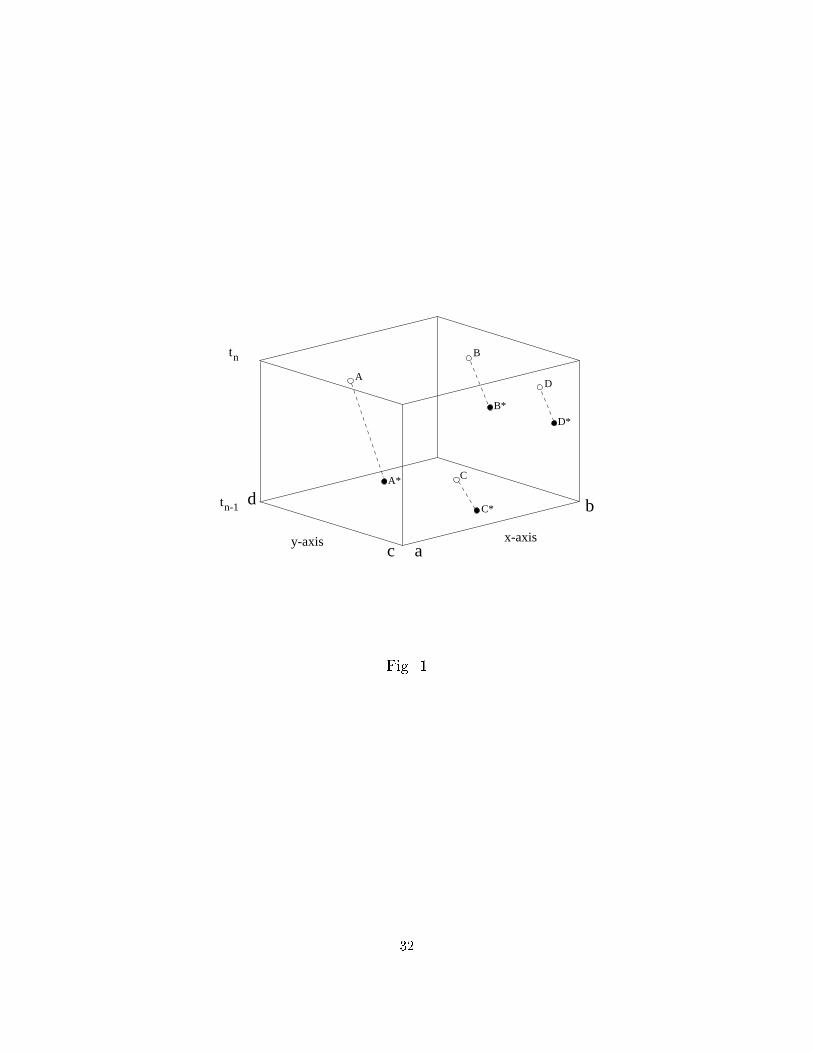
B

y-axis x-axis

tn

D

C

dn-1t

c a

b

A*

A

B*

D*

C*

Fig. 1

32

−1 −0.8 −0.6 −0.4 −0.2 0 0.2 0.4 0.6 0.8 1−0.4

−0.2

0

0.2

0.4

0.6

0.8

1

1.2

1.4

x−axis

QP

G te

st fu

nctio

ns

"−." GAL; "−−" QPG, V=1, D=0.3; "−" QPG, V=1, D=0.0001

−1 −0.8 −0.6 −0.4 −0.2 0 0.2 0.4 0.6 0.8 1−0.4

−0.2

0

0.2

0.4

0.6

0.8

1

1.2

1.4

x−axis

CP

G te

st fu

nctio

ns

"−." GAL; "−−" CPG, Cu=0.5; "−" CPG, Cu=1

Fig 2a. QPG test functions. Fig 2b. CPG test functions.

0 0.2 0.4 0.6 0.8 1 1.2−0.4

−0.2

0

0.2

0.4

0.6

0.8

1

x−axis

solu

tions

"−" initl cond & anl, "− −" B−E−GAL, "o" B−E−QPG, "x" B−E−CPG

dt = 1/100

dt = 1/20

0 0.2 0.4 0.6 0.8 1 1.2−0.4

−0.2

0

0.2

0.4

0.6

0.8

1

x−axis

solu

tions

"−" anl, "−−" B−E−GAL, "o" B−E−QPG, "x" B−E−CPG, dt = 1/300

Fig 3. B-E Schemes, �x = 160, �t = 1

20& 1

100Fig 4. B-E Schemes, �x = 1

60, �t = 1

300

33

0 0.2 0.4 0.6 0.8 1 1.2−0.4

−0.2

0

0.2

0.4

0.6

0.8

1

x−axis

solu

tions

"−" anl, "−−" B−E−GAL, "o" B−E−QPG, "x" B−E−CPG, dt = 1/1000

0 0.2 0.4 0.6 0.8 1 1.2−0.4

−0.2

0

0.2

0.4

0.6

0.8

1

x−axis

solu

tions

"−" initl cond & anl, "−−" C−N−GAL, "o" C−N−QPG, "−." ELLAM, dt=1/20

Fig 5. B-E Schemes, �x = 160, �t = 1

1000Fig 6. C-N/ELLAMSchemes, �x = 1

60, �t = 1

20

0 0.2 0.4 0.6 0.8 1 1.2−0.4

−0.2

0

0.2

0.4

0.6

0.8

1

x−axis

solu

tions

"−" anl, "−−" C−N−GAL, "o" C−N−QPG, "x" C−N−CPG, dt=1/100

0 0.2 0.4 0.6 0.8 1 1.2−0.4

−0.2

0

0.2

0.4

0.6

0.8

1

x−axis

solu

tions

"−" anl, "−−" C−N−GAL, "o" C−N−QPG, "x" C−N−CPG, dt=1/400

Fig 7. C-N Schemes, �x = 160, �t = 1

100Fig 8. C-N Schemes, �x = 1

60, �t = 1

400

34

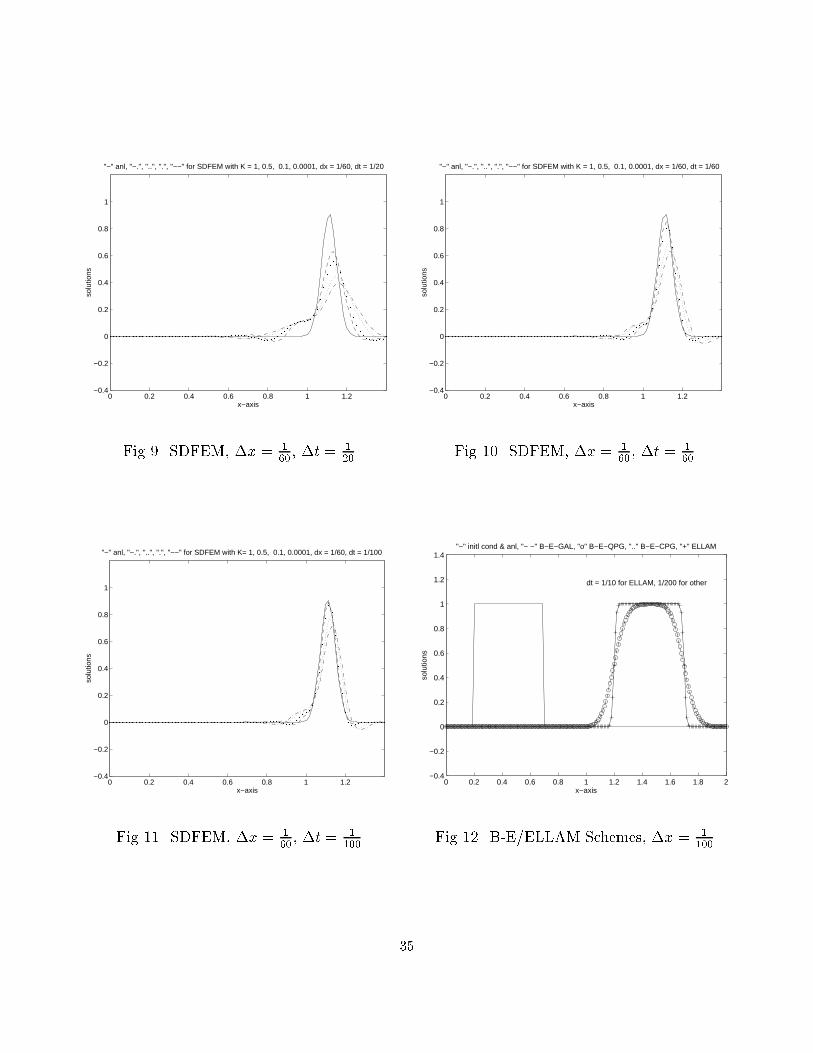
0 0.2 0.4 0.6 0.8 1 1.2−0.4

−0.2

0

0.2

0.4

0.6

0.8

1

x−axis

solu

tions

"−" anl, "−.", "..", ".", "−−" for SDFEM with K = 1, 0.5, 0.1, 0.0001, dx = 1/60, dt = 1/20

0 0.2 0.4 0.6 0.8 1 1.2−0.4

−0.2

0

0.2

0.4

0.6

0.8

1

x−axis

solu

tions

"−" anl, "−.", "..", ".", "−−" for SDFEM with K = 1, 0.5, 0.1, 0.0001, dx = 1/60, dt = 1/60

Fig 9. SDFEM, �x = 160, �t = 1

20Fig 10. SDFEM, �x = 1

60, �t = 1

60

0 0.2 0.4 0.6 0.8 1 1.2−0.4

−0.2

0

0.2

0.4

0.6

0.8

1

x−axis

solu

tions

"−" anl, "−.", "..", ".", "−−" for SDFEM with K= 1, 0.5, 0.1, 0.0001, dx = 1/60, dt = 1/100

0 0.2 0.4 0.6 0.8 1 1.2 1.4 1.6 1.8 2−0.4

−0.2

0

0.2

0.4

0.6

0.8

1

1.2

1.4

x−axis

solu

tions

"−" initl cond & anl, "− −" B−E−GAL, "o" B−E−QPG, ".." B−E−CPG, "+" ELLAM

dt = 1/10 for ELLAM, 1/200 for other

Fig 11. SDFEM, �x = 160, �t = 1

100Fig 12. B-E/ELLAM Schemes, �x = 1

100

35

0 0.2 0.4 0.6 0.8 1 1.2 1.4 1.6 1.8 2−0.4

−0.2

0

0.2

0.4

0.6

0.8

1

1.2

1.4

x−axis

solu

tions

"−" anl, "− −" B−E−GAL, "o" B−E−QPG, ".." B−E−CPG, dt = 1/800

0 0.2 0.4 0.6 0.8 1 1.2 1.4 1.6 1.8 2−0.4

−0.2

0

0.2

0.4

0.6

0.8

1

1.2

1.4

x−axis

solu

tions

"−" anl, "− −" B−E−GAL, "o" B−E−QPG, ".." B−E−CPG, dt = 1/2000

Fig 13. B-E Schemes, �x = 1100

, �t = 1800

Fig 14. B-E Schemes, �x = 1100

, �t = 12000

0 0.2 0.4 0.6 0.8 1 1.2 1.4 1.6 1.8 2−0.4

−0.2

0

0.2

0.4

0.6

0.8

1

1.2

1.4

x−axis

solu

tions

"−." C−N−GAL, "− −" C−N−QPG, "−" C−N−CPG, dt=1/100

0 0.2 0.4 0.6 0.8 1 1.2 1.4 1.6 1.8 2−0.4

−0.2

0

0.2

0.4

0.6

0.8

1

1.2

1.4

x−axis

solu

tions

"−." C−N−GAL, "− −" C−N−QPG, "−" C−N−CPG, dt=1/200

Fig 15. C-N Schemes, �x = 1100

, �t = 1100

Fig 16. C-N Schemes, �x = 1100

, �t = 1200

36

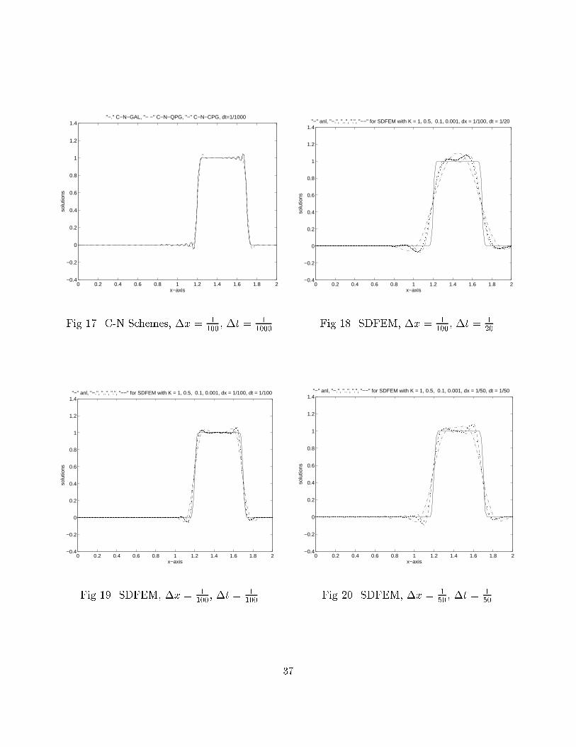
0 0.2 0.4 0.6 0.8 1 1.2 1.4 1.6 1.8 2−0.4

−0.2

0

0.2

0.4

0.6

0.8

1

1.2

1.4

x−axis

solu

tions

"−." C−N−GAL, "− −" C−N−QPG, "−" C−N−CPG, dt=1/1000

0 0.2 0.4 0.6 0.8 1 1.2 1.4 1.6 1.8 2−0.4

−0.2

0

0.2

0.4

0.6

0.8

1

1.2

1.4

x−axis

solu

tions

"−" anl, "−.", "..", ".", "−−" for SDFEM with K = 1, 0.5, 0.1, 0.001, dx = 1/100, dt = 1/20

Fig 17. C-N Schemes, �x = 1100

, �t = 11000

Fig 18. SDFEM, �x = 1100

, �t = 120

0 0.2 0.4 0.6 0.8 1 1.2 1.4 1.6 1.8 2−0.4

−0.2

0

0.2

0.4

0.6

0.8

1

1.2

1.4

x−axis

solu

tions

"−" anl, "−.", "..", ".", "−−" for SDFEM with K = 1, 0.5, 0.1, 0.001, dx = 1/100, dt = 1/100

0 0.2 0.4 0.6 0.8 1 1.2 1.4 1.6 1.8 2−0.4

−0.2

0

0.2

0.4

0.6

0.8

1

1.2

1.4

x−axis

solu

tions

"−" anl, "−.", "..", ".", "−−" for SDFEM with K = 1, 0.5, 0.1, 0.001, dx = 1/50, dt = 1/50

Fig 19. SDFEM, �x = 1100

, �t = 1100

Fig 20. SDFEM, �x = 150, �t = 1

50

37

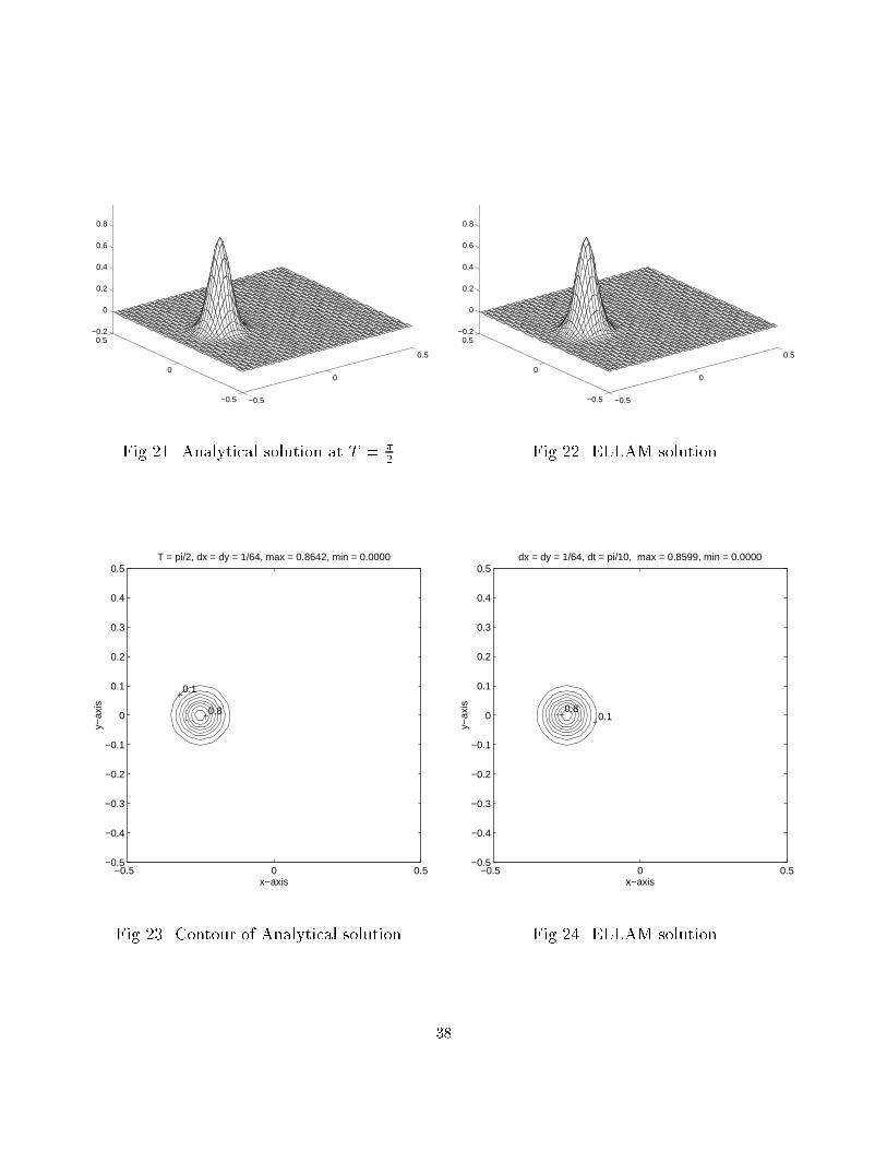
−0.5

0

0.5

−0.5

0

0.5−0.2

0

0.2

0.4

0.6

0.8

−0.5

0

0.5

−0.5

0

0.5−0.2

0

0.2

0.4

0.6

0.8

Fig 21. Analytical solution at T = �2. Fig 22. ELLAM solution.

−0.5 0 0.5−0.5

−0.4

−0.3

−0.2

−0.1

0

0.1

0.2

0.3

0.4

0.5T = pi/2, dx = dy = 1/64, max = 0.8642, min = 0.0000

x−axis

y−ax

is

0.1

0.8

−0.5 0 0.5−0.5

−0.4

−0.3

−0.2

−0.1

0

0.1

0.2

0.3

0.4

0.5dx = dy = 1/64, dt = pi/10, max = 0.8599, min = 0.0000

x−axis

y−ax

is

0.1 0.8

Fig 23. Contour of Analytical solution. Fig 24. ELLAM solution.

38